In contrast with a long tradition of economic history studies focused on the increasing participation of Mexico in the international economy during the Porfiriato (1876–1910), this work deals with a relevant and debatable aspect of the domestic sector: the integration of agricultural markets. This issue is closely connected with the major role that railroads, the fundamental innovation in transportation during the period, played in the Mexican economy.
The main purpose of the study is to provide another view not only of these topics but also of a decisive period of modern Mexican history. Convergence of prices is considered a genuine manifestation of market integration. Because corn became the staple of commercial agriculture, as well as the main subsistence crop, it deserves on its own merits to play the leading role in any story about the integration of agricultural markets in pre-industrial Mexico.1
Coatsworth, La Producción.
We hypothesize that: given Mexican geography, railroads inevitably stimulated the economic integration of the Mexican states; as a result, interstate differentials in corn prices might have experienced a substantial reduction during the
pax porfiriana. This hypothesis had not yet been statistically tested in the literature. Through panel techniques, following the methodology of Robert Barro and Xavier Sala-i-Martin, we analyze the convergence of corn prices across Mexican states and territories—hereafter states—between 1885 and 1908.
2 Barro and Sala-i-Martín, “Economic Growth,” “Convergence,” and Economic Growth.
It is our main conclusion that interstate differentials in corn prices substantially decreased in Porfirian Mexico and that railroads played a significant and positive role in the process of convergence. Thus, on the eve of the Mexican Revolution, corn market integration had reached a historical maximum.
The authoritative research undertaken by John Coatsworth established a new interpretation of the relations between railroads, economic growth, and markets in Porfirian Mexico.3
Coatsworth, “Indispensible Railroads” and El Impacto.
Although the backward linkages resulting from the operation of railroads were scarce, or null, their contribution to the economic growth of the period in terms of social savings was
crucial: no less than 50 percent of the increase in per capita gross domestic product between 1880 and 1910. Thus, railroads were
indispensable for economic growth in Mexico.
4 Summerhill (Transport Improvements) has emphasized the “unprecedented by international standards” importance of Mexican—and Brazilian—railroads to the transition to economic growth by the end of the nineteenth century.
However, the main beneficiaries of the new possibilities offered by the improvement in overland transport were firms engaged in import-export activities, foreign mining companies in particular. Railroads are then inseparable from the increasing export orientation of the Mexican economy and the parallel change in its output mix. This picture might imply that the domestic sector of the Mexican economy, in spite of its larger size, could only make a relatively minor use of railroads. Even though Coatsworth's research on railroads recognizes the considerable quantity of agricultural products transported for home consumption, it emphasized their contribution to the export sector.
5 Echoes of the formerly influential dependentist thought, lately criticized by Haber (“Introduction”), might be perceptible in this point.
Sandra Kuntz and Paolo Riguzzi have complemented the work by Coatsworth.6
Kuntz, Empresa, “Mercado,” “Ferrocarriles y Mercado: Tarifas,” “Los Ferrocarriles,” and “Ferrocarriles y Mercado de Productos”; and Riguzzi, “Mercados.”
All in all they put forward a basically “optimistic” reconsideration of the impact of railroads on the domestic economic integration of Mexico. A closer examination of the traffic (origin, destination, composition, short lines, and so on) reveals that: far from exclusively reinforcing or creating export-oriented enclaves, the railroad network linked the main and most dynamic production and consumption centers; and exports only represented a small fraction of total freight. Hence, the idea that railroads stimulated agricultural market integration across Mexican states is perfectly plausible. In fact, Kuntz shows that corn, wheat, and other agricultural products intended for the domestic market accounted for a significant part of the
Ferrocarril Central shipments between 1884 and 1907.
7 However, Kuntz claims that corn, the only product that could have led the process of national market integration was too cheap to fully exploit the advantages of the new means of transportation, in spite of the relatively rather rapid decline in its freight rates.
8 Kuntz, “Ferrocarriles y Mercado de Productos.”
Thus, the national market remained
fragmented.
9 “On account of the magnitude of its production and the generalized character of its consumption, corn could have behaved as the product leading the formation of a national market of agricultural products; but owing to the conditions under which it was cultivated and its low price, it proved to be unable to play that role. This combination turned out to be fateful for the nineteenth-century Mexican economy: it obstructed the formation of wide and deep commercial circuits; it hindered the economy's specialization, and it kept a considerable part of the population outside the marketplace.” Kuntz (“Ferrocarriles y Mercado de Productos,” p. 480). Translated from Spanish by the authors.
This optimism about the role played by railroads is not a completely novel idea. As Aurora Gómez Galbarriato has recently pointed out, Francisco Calderón had already put forward an essentially optimistic version of the effects of railroads on the integration of the domestic sector.10
“Optimism” also characterizes Mario Cerruti's view on the positive consequences of railroads for integration at the regional, national and international levels of the dynamic “north system” of states.
11 Cerruti's (Burguesia) “north system: consists of the states of Coahuila, Nuevo León y Tamaulipas as well as important parts of San Luís Potosí, Zacatecas, Durango y Chihuahua.
To some extent, this article attempts to take a step further into finding the answer to one of the puzzles in Mexican economic history identified by Noel Maurer.12
According to Maurer, “the railroads appear to have contributed mightily to the nation's economic growth in the late 19th and early 20th centuries.”
13 Testing with statistical rigor the falsifiable hypothesis of the railroads' stimulus to corn price equalization in Porfirian Mexico, we hope to reinforce Maurer's confidence in the accuracy of his “apparent optimism.” Additionally, Maurer reminds us of “the relative dearth of economically literate studies of agriculture in the Nineteenth Century.”
14 From a methodological viewpoint, our analysis is original because it relies on the estimation of a panel data model.15
Our approach connects with an increasing international scholarship in the field of integration of national markets. The interesting findings of a “first generation” of scholars were mostly based on rather simple statistical tools (Metzer, “Railroad Development”; Hurd, “Railways”; and Rothenberg, “Market”). On the contrary, some authors among those of the “second generation” use the much more sophisticated techniques represented by time-series analysis (Roehner, “Les Mechanismes”; Chevet, “National and Regional Corn Markets”; Persson, Grain Markets; Ejrnaes and Persson, “Market Integration”; and Llopis and Jerez, “El Mercado”).
Our strategy consisted of studying the convergence of corn prices across the 30 states composing the Mexican Republic between 1885 and 1908. Prices used are those published by Instituto Nacional de Estadística, Geografía e Informática (hereafter INEGI).
16 As is more often than not the case in economic history research, the prestatistical criteria used for the original gathering of those prices make them probably far from perfect. But some unavoidable imperfections do not justify their automatic disqualification. Moreover, after close examination of the results obtained from unprejudiced work on them, we find that they may at most be affected only by certain deficiencies that do not seriously distort the general picture of the corn prices convergence process.
A FIRST EXPLORATION OF DATA
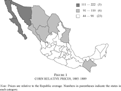
This section begins with a geographical approach to prices. Figure 1 depicts the distribution of prices across Mexican states in 1885–1889.17
In this section, unless otherwise indicated, prices are always relative to the Republic average.
CORN RELATIVE PRICES, 1885–1889
It shows a clear pattern: expensive corn is a northern phenomenon with the only exception being Chiapas, in the south. In most states, corn prices are below the national average. Differences in prices among states may be considerable: a factor of five between the most expensive state and the cheapest one (Baja California and Campeche, respectively); a factor of four between the three most expensive states and the three cheapest ones (Baja California, Sonora, and Chiapas and Campeche, Colima, and Tepic—currently Nayarit, respectively).
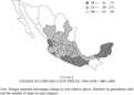
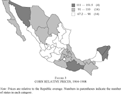
Figure 2 shows the change in relative corn prices between 1885 and 1908. Corn prices follow a peculiar pattern of change. In general, corn prices decrease in all previously expensive states whereas they increase in the initially cheap states or experience a relatively small change in the rest of states. This pattern brought about significant changes in the geography of prices. In 1904–1908 the geographical distribution of prices (see Figure 3) was still heterogeneous, but a process of equalization had been well under way for some time.
CHANGE IN CORN RELATIVE PRICES, 1904–1908/1885–1889
CORN RELATIVE PRICES, 1904–1908
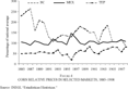
The aggregate situation in 1904–1908 resulted from a number of different trajectories proceeding from 1885. For the sake of simplicity, Figure 4 shows three single representative trajectories: Baja California (downward trend), Mexico (moving closely around the national simple average) and Tepic (upward trend).
CORN RELATIVE PRICES IN SELECTED MARKETS, 1885–1908
Figure 4 shows striking differences in corn prices across states at the beginning of the period under consideration and their gradual reduction in the course of time. However, behind the apparent reduction in price dispersion we find a basic dissimilarity: some of the trajectories depicted on Figure 4 (such as those of Baja California and Tepic) may be considered signs of a tendency towards convergence in some of the Mexican regions, whereas that of Mexico suggests that other regions might have already made up an integrated corn market. This mixed situation reflects the different starting-off times in the race for closer integration in so big and segmented a country as Mexico.
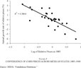
Continuing this first exploration of data, Figure 5 is intended to show the β-convergence in the cross section of states, that is, whether or not prices in the lower-priced states grew faster than they did in the higher-priced states. Given the existence of a negative and statistically significant relationship between the initial price level and price growth, the hypothesis of β-convergence cannot be ruled out.
CONVERGENCE OF CORN PRICES ACROSS MEXICAN STATES, 1885–1908
However, β-convergence is a necessary, but not sufficient, condition for σ-convergence.18
Barro and Sala-i-Martín, Economic Growth.
But market integration—either national (Jacob Metzer and John Hurd) or international (Kevin O'Rourke and Jeffrey Williamson and Ronald Findlay and O'Rourke)—requires a decrease in price dispersion.
19 Metzer, “Railroad Development”; and Hurd, “Railways”; O'Rourke and Williamson, Globalization; and Findlay and O'Rourke, “Commodity Market Integration.”
Therefore, we test for σ-convergence.
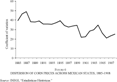
Figure 6 reveals the existence of σ-convergence: between 1885 and 1908, the dispersion of corn prices across Mexican states was reduced almost by half.
DISPERSION OF CORN PRICES ACROSS MEXICAN STATES, 1885–1908
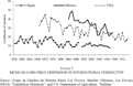
By 1908 the dispersion was still high but not so high as to be considered exceptional. In fact, since late in the nineteenth century corn price dispersion in Mexico was similar to that in the United States, and its reduction in 1885–1908 was even faster (see Figure 7).20
U.S. corn prices have been taken from United States Department of Agriculture, “Bulletin.” States included are those for which there are continuous data from 1869 to 1915 (Alabama, Arkansas, California, Connecticut, Delaware, Florida, Georgia, Illinois, Indiana, Iowa, Kansas, Kentucky, Louisiana, Maine, Maryland, Massachusetts, Michigan, Minnesota, Mississippi, Missouri, Nebraska, New Hampshire, New Jersey, New York, North Carolina, Ohio, Oregon, Pennsylvania, Rhode Island, South Carolina, Tennessee, Texas, Vermont, Virginia, Wisconsin, and Virginia). Working with 40 states (the 36 mentioned plus Colorado, North Dakota, South Dakota, and Utah) with data on corn prices for 1885–1908, the results are basically identical.
Certainly, the physical dimension of the U.S. market is much bigger, but Mexico's northern neighbor enjoyed a more developed economy in which transportation faced fewer technical and geographical obstacles.
MEXICAN CORN PRICE DISPERSION IN INTERNATIONAL PERSPECTIVE
At the same time, when compared with Spain, Mexican dispersion always appears to be substantially wider (see Figure 7).21
Sources of Spanish data are Sánchez Albornoz, Los Precios Agrícolas; and Grupo de Estudios de Historia Rural, Los Precios. They cover the 48 provinces in peninsular Spain and the Balearic Islands. For every year from 1856 to 1889, the series include all the provinces. After 1891, some provinces may be absent, but never more than two of them except in 1904.
However, the dispersion of wheat prices in Spain was influenced by more favorable geographical features (500,000 square kilometers versus 2 million and a rounded shape that permitted an intense coastal navigation) and the availability of a nationwide railroad network since the 1860s. As the comparison with Spain and the United States suggests, the Mexican case is not a peculiar one.
22 Moreover, apart from its relatively late start, it is coincident with numerous national experiences (such as those of Germany, India, and Russia) in the second half of the nineteenth century, as well as with international experience, see O'Rourke and Williamson, Globalization.
Regions and Convergence
In the late nineteenth and early twentieth centuries Mexico was—and still is—a very heterogeneous country. Differences across regions in terms of geography, economy, and ethnicity were enormous. Consequently, it is reasonable to assume a priori that the participation of the various regions in the integration process should have been uneven. The simple fact that the railroad network did not cover the whole country lends support to that hypothesis. Thus, we proceed in this section by studying the convergence of corn prices across and within groups of states. The groups into which Mexico is divided are those considered by Angel Bassols,23
Bassols, Geografía. North-western region: Baja California, Sinaloa, Sonora and Tepic. Northern region: Chihuahua, Cohauila, Durango, San Luís Potosí and Zacatecas. North-eastern region: Nuevo León and Tamaulipas. Central-western region: Aguascalientes, Colima, Guanajuato, Jalisco and Michoacán. Central-eastern region: Distrito Federal, Hidalgo, Mé xico, Morelos, Puebla, Querétaro y Tlaxcala. Southern region: Chiapas, Guerrero and Oaxaca. Eastern region: Tabasco and Veracruz. Yucatán peninsula region: Campeche and Yucatán.
Gerardo Esquivel,
24 Esquivel, “Convergencia.” Capital: Distrito Federal and México. Center: Hidalgo, Morelos, Puebla and Tlaxcala. Center-North: Aguacaliantes, Durango, Querétaro, San Lu ís Potosí and Zacatecas. Gulf: Campeche, Tabasco, Veracruz and Yucatán. North: Baja California, Chihuahua, Coahuila, Nuevo León, Sonora and Tamaulipas. Pacific: Colima, Jalisco, Sinaloa and Tepic. South: Chiapas, Guerrero, Michoacán and Oaxaca.
and INEGI.
25 INEGI, “Estadísticas.” North: Chihuahua, Coahuila, Durango, Nuevo León, San Luís Potos í and Tamaulipas. Gulf: Campeche, Tabasco, Veracruz and Yucatán. Northern Pacific: Baja California, Sinaloa, Sonora and Tepic. Southern Pacific: Chiapas, Colima, Guerrero and Oaxaca. Centre: Aguascalientes, Distrito Federal, Guanajuato, Hidalgo, Jalisco, México, Michoacán, Morelos, Puebla, Querétaro and Tlaxcala.
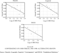
We work with three alternative divisions of Mexican geography to minimize the bias that might result from the grouping of states. We find evidence supporting both β-convergence and σ-convergence of corn prices across Mexican regions (see
Figures 8 and
9).
CONVERGENCE OF CORN PRICES, 1985–1908: ALTERNATIVE GROUPS
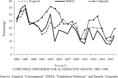
CORN PRICE DISPERSION FOR ALTERNATIVE GROUPS, 1885–1908
Between 1885 and 1908 a clear process of equalization in regional prices took place. An interesting—and complementary—picture emerges if we look at convergence within groups. Once again, results are consistent no matter which geographical division of Mexico is considered. Not surprisingly, the circumstances and the pace of the convergence in corn prices differ considerably within groups of states.
Three different patterns may be identified. First, regions such as Yucatan, according to Bassols's classification, and Gulf, in those of Esquivel and INEGI, show practically no σ-convergence. Their coefficients of variation are initially high and decline very slightly or not at all. Second, a central area (Bassols's Central-eastern region, Esquivel's and INEGI's Central regions and Esquivel's Central-northern region) is characterized by a relatively low initial level of dispersion and slow progress in σ-convergence afterwards. Finally, the rest of the regions always show a more-or-less high level of initial dispersion and different rhythms of σ-convergence. In INEGI's Southern Pacific, Bassols's Southern and North-eastern and Esquivel's Pacific regions, the fall in dispersion was especially steep. In short, with the exception of the Yucatan and Gulf groups, dispersion of corn prices within groups was already low by the mid 1880s or decreased at different—never too slow—paces in subsequent years.
The complexity of some regional trajectories is also perceptible through the existence of: a fairly integrated “border economy” constituted by Mexican and American border states;26
The slope of the β-convergence equation is −0.033, with a t-statistic of 5.303, an R-squared coefficient of 0.800 and the coefficient of variation falling from 45 in 1885–1886 to 25 in 1907–1908. Arizona is excluded because there are no data available.
and a weaker integration between the two geographical extremes of the Mexican Republic.
27 The slope of the β-convergence equation is −0.028, with a standard deviation of 3.042, an R-squared coefficient of 0.507 and the coefficient of variation falling from 51 in 1885–1887 to 37 in 1906–1908. In this exercise, we are considering the following states: Baja California, Sonora, Coahuila, Chihuahua, Tamaulipas, Chiapas, Campeche, and Yucatan.
The picture of the Mexican corn market emerging from this first exploration of data is that of equalization in prices across states. Thus, increasing integration of the domestic market for the main and cheapest agricultural commodity, similar to that observed in the countries participating in the globalization process of the last decades of the nineteenth century, also applies to Mexico. We also find different patterns at sub-national level: some central regions seem to be integrated before 1885, others experience a more-or-less rapid convergence—even within a transnational “border economy”—and southeastern states do not converge at all. Hence, inter-regional heterogeneity is a feature of the corn market integration process in Porfirian Mexico. Interestingly enough, the internal coherence of the national panorama is not seriously affected by abnormal, disturbing data. This fact increases our confidence in the data set we are using. However, the relatively simple statistical techniques used so far do not make it possible to find an answer to some relevant questions, such as, Which are the sources of the inter-regional heterogeneity?; and What is the role of railroads in the integration process? Therefore we turn to panel data techniques in the next section.
A MODEL OF CONVERGENCE
We begin this section by briefly describing the convergence model and first estimations. Next, we focus our attention on steady-state heterogeneity. We put off the discussion about the relationship between railroads and the integration process to the next section. The methodology used in this study is similar to the one proposed by Barro and Sala-i-Martín.
28 Barro and Sala-i-Martín, “Economic Growth,” “Convergence,” and Economic Growth.
The econometric model is
where 30 and 24 are, respectively, the cross-section and the time dimensions of the panel, Pi, t is the corn price for the ith state at period t, and
is the corn price average for the Republic at period t; therefore, pi, t is the relative corn price with respect to the Republic average at period t for the ith state. βi measures the reaction of the current price growth rate to past corn price level; αi is a 1 × 1 scalar representing the effects of those variables peculiar to the ith state, which are assumed to be constant over time, but they might differ across states. The error term εi, t is a stochastic input, peculiar to each state and time period, representing the effect of variables of minor importance that directly affect the growth rate of prices. A steady state is defined as an equilibrium path where relative prices remain constant over time. Imposing εi, t = 0 and pi, t = pi, t − 1=pi* for all i, t in equation 1, yields
These steady states are stable or unstable depending on βi. Values of βi closer to one are associated with a fast convergence process; values of βi approaching zero indicate slower and monotonic convergence. Finally, values of βi close to two also show slower convergence, although accompanied by oscillating behavior. Given βi ∈ (0,2), those states with αi = 0 are converging on the Republic average, whereas those with αi > (<) 0 are converging above (below) the Republic average.
Preliminary Convergence Results
The specification of the convergence model in equation 1 responds to a logical sequence:29
first we check whether or not the fixed-effect model is appropriate;
30 We use the Hausman (“Specification Tests”) test to discriminate between the stochastic and deterministic nature of αi in equation 1.
second, we reject the existence of common fixed effects across states;
31 The p-value of the suitable Wald F-test is 0.0001.
finally, we also reject that slopes are equal for all states.
32 The p-value of the suitable Wald F-test is 0.001. In the convergence literature, it is common to impose equality among β coefficients. However, this assumption is not justified in our case, and we must consider this fact in the econometric model in order to be more accurate in the convergence analysis.
and
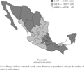
11, respectively, depict the heterogeneity in steady states and speeds of convergence across Mexican states.
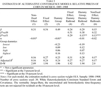
Table 1 summarizes the estimation of several econometric models. Just for illustrative purposes, the first column shows the results of equation 1 with common α and β for all states. The second column shows the fixed-effect model, with common β and different α. The rest of columns show alternative models that are described in what follows.
In all cases, the estimated levels of β reinforce the β-convergence hypothesis: the price of corn in states where it was relatively far below its own steady state in 1885 tended to grow faster than in states where the price was initially closer to its steady state and vice versa. However, according to previous results, we do not find evidence supporting: absolute convergence, for it implies a common price level which all states were approaching; or identical convergence speeds across Mexican states. These findings reinforce the picture of heterogeneity across regions and states.
Steady-State Heterogeneity
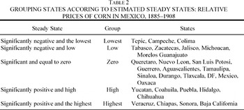
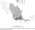
Because we have found convincing evidence against the unconditional convergence hypothesis and in support of the conditional one, the steady-state heterogeneity must be seriously taken into account. Arguably, some intelligible pattern might underlie this steady-state heterogeneity: likely, states with similar geographical and economic characteristics were approaching nearby steady states (see Figure 10). With only a few exceptions, Figure 10 shows a picture that closely resembles that of a nearly perfect center-periphery structure: states converging on the Republic average or slightly below are located in a wide, almost vertically oriented, central strip, including from Nuevo Leon and Tamaulipas at the top to Michoacan and Guerrero at the bottom; states converging on the highest steady states constitute two compact areas “surrounding” the central strip; states converging on the lowest steady states are small and sparsely populated and situated on both the Pacific and the Caribbean shores. In Table 2 Mexican states are classified according to their similarities in estimated steady states.33
We classify steady states, s, following a statistical criteria. From equation 1, and setting different α and β for each state,
for all i = 1, 2, …, 30. Its sample average is
and its standard deviation is
. According to the Jarque-Bera test, the series of
is normally distributed (the p-value is 0.48). Hence, if
(an 85-percent one-tail confidence bound), the ith state belongs to the highest group; if
, the ith state belongs to the higher group; if
, to the lower group, and if
to the lowest group. Those states with
belong to the group converging on the sample average.
This classification shows a slightly different picture from—although consistent with— the one depicted in
Figure 10.
This sort of heterogeneity may be captured in equation 1, adding four regional dummies (we call this model in Table 1 “dummy group”: lowesti = 1, with i equal to Tepic, Campeche, and Colima, and zero otherwise; lowi = 1, with i equal to Tabasco, Zacatecas, Jalisco, Michoacán, Morelos, and Guanajuato, and zero otherwise; highi = 1, with i equal to Yucatan, Coahuila, Puebla, Hidalgo, and Oaxaca, and zero otherwise; and highesti = 1, with i associated with Veracruz, Chiapas, Sonora, and Baja California, and zero otherwise. The resulting model is
The estimation of equation 3 shows (column 3 in Table 1) that many central—loosely defined—states (such as Guerrero, Aguascalientes, Mexico, DF, etc.) were converging to the Republic average or very close to it, whereas corn prices in the group of “small and coastal states” (such as Tepic, Campeche, and Colima) were moving towards a much lower steady state (40–60 percent) than that of the “central region.” Other states (such as Baja California, Chihuahua, Sonora, Veracruz, etc.) were converging on a very high steady state (40 percent above the Republic average). Certainly, these differences are far from negligible but they were significantly smaller than those existing circa 1885.34
Even though an analysis in depth is beyond the limits of this work, steady states heterogeneity deserves some exploration. It seems reasonable to expect some interaction between market conditions (supply and demand) and steady-state levels within states. However, because of the limitations of the data available, we found it difficult to correctly measure the market conditions associated with a given state. We have information on production and population circa 1907 for each state (Yi and Ni, respectively, for I = 1, 2, …, 30). However, data for consumption are not available. Assuming that, in terms of corn, Mexico may be considered a closed economy, total corn production—in per capita units—must be pretty close to consumption. Thus, we can compute the ratio of total production to total population, which must be similar to the total consumption/population ratio, let us call it X. If we multiply X by each state's population, we have a proxy of consumption for each state, let us call it Ci. Hence, now we have data to construct a proxy for production per capita surplus for each state: (Yi − Ci)/Ni. Circa 1907 states producing important surplus of corn were Guerrero, Mexico, Morelos, Guanajuato, Nuevo Leon, Michoacan, and Campeche, while Baja California, Sonora, Distrito Federal, Coahuila, Oaxaca, and Puebla show deficits. We found that this proxy is an additional significant variable in explaining the corn price growth rate. Therefore, as expected, surpluses are, on average, associated with lower steadystates.
RAILROADS AND THE INTEGRATION PROCESS
In Porfirian Mexico prices of the main agricultural product experienced a convergence process, as was the rule rather than the exception in countries involved in the growing international economic integration during the second half of the nineteenth century. However, as shown in the preceding section, this process was of a peculiar kind: Mexican states converged on different price levels at various speeds of convergence. In this section, we examine the role of railroads in the particular process of corn market integration experienced by Porfirian Mexico. O'Rourke and Williamson have emphasized the major role of declining transport costs within national markets “for both the development of national economies and the world economy.”35
O'Rourke and Jeffrey Williamson, Globalization, p. 41.
The contribution of railroads to market integration in the United States, Russia, India, Germany, or France is well documented.
36 O'Rourke and Jeffrey Williamson, Globalization.
In Porfirian Mexico, the most conspicuous transport innovation was the comparatively late and rapid construction of the railroad network: 1,100 kilometers in 1880 compared with 20,000 in 1910.
37 Coatsworth, El Impacto, p. 36.
Coatsworth's “geographical conspiracy” (the absence of cheap alternatives and the location of the most populated areas far from both shores) explains the enormous impact of railroads on transport costs.
38 Coatsworth, El Impacto. Towards 1889 the cost of transport of agricultural products by railroad were generally half of those of the cheapest alternative option (Kuntz, “Ferrocarriles y Mercado de Pruductos,” p. 478). One more indication of the potential of railroads for market integration in Mexico is given by these data: circa 1850 corn consumed in Guanajuato was usually produced within a radius of about 55 kilometers of the town; a longer distance raised transportation costs up to 40 percent of the final price (Bushnell and Macaulay, El Nacimiento, p. 68).
However, apart from the general rather pessimistic opinion of Coatsworth, little analytical work—as Kuntz has pointed out—has been devoted to the role of railroads in the integration of a national market for agricultural products in Mexico.39
Kuntz, “Los Ferrocarriles.”
Certainly, recent research by Kuntz and Riguzzi show a more optimistic view of railroads as an important factor in market integration.
40 Kuntz, Empresa, “Mercado,” “Ferrocarriles y Mercado: Tarifas,” “Los Ferrocarriles,” and “Ferrocarriles y Mercado de Productos”; and Riguzzi, “Mercados.”
However, this optimism is only conditional because the exercise in the “potential contribution” of railroads to corn market integration done by Kuntz concludes with a rather pessimistic view.
41 Kuntz, “Ferrocarriles y Mercado de Productos.”
The low price of corn implied a low “tolerance” of corn to transport costs that limited the extension of the market. Her estimation of the “effective contribution” is also pessimistic as far as corn is concerned: only 20 percent of the domestic production plus imports was transported by rail in 1907. Kunzt's pessimism about corn is in contradiction with our findings suggesting a generalized trend towards price equalization across Mexican states. Her view is also opposed to the unambiguously positive role played by railroads in market integration in other countries.
Our attempt to clear up this contradiction begins by introducing railroads in our empirical framework. We have not been able to find any clear relationship between railroads and steady states: for instance, Tabasco's was among the lowest whereas that of Baja California was well above the national average; Veracruz, Puebla, Hidalgo, Mexico, and Federal District, all of them with a relatively early presence of railroads, show a relatively wide range of steady states. However, the geography depicted in Figure 11 suggests that the timing and the scope of the diffusion of railroads across Mexico should be considered in the explanation of the interstate variability of speeds of convergence. Thus, we try to capture the effect of railroads on convergence speeds by estimating the dummy railroad model
where rail0 and rail1 are railroad-dummies, with rail0i = 1, for i associated with states with a railroad before 1885 (Aguascalientes, Chihuahua, Distrito Federal, Durango, Guanajuato, Hidalgo, Jalisco, Mexico, Michoacán, Morelos, Puebla, Queretaro, Tlaxcala, Veracruz, and Zacatecas), and zero otherwise; rail1i = 1, for i associated with states where the railroad was build or connected with the main network between 1885 and 1908 (Chiapas, Coahuila, Colima, Guerrero, Nuevo León, Oaxaca, San Luis Potosi, Tamaulipas, and Tepic) and zero otherwise.
42 Parameters in equation 4 turn out to be highly significant—see column 4 in
Table 1.
In order to obtain more precise estimations of the β, we combine equations 3 and 4
Parameters, with the exception of α1 (see column 5 in Table 1), are highly significant as well, and the railroad-related variables bear the expected sign. Finally, column 6 in Table 1 shows the estimation of a new model. This model, although similar to equation 5, has a common constant term for each state. Convergence results might be biased because of the inclusion of fixed effects in the panel regression (as in equations 4 and 5). However, after comparing results in columns 4, 5, and 6, we may disregard this possibility and feel more confident about the robustness of our main conclusions: the existence of corn price convergence across states; and that railroads played a significant and positive role in increasing the speed of such convergence process.
Interpretation of Results
The speed of convergence of those states with railroads in 1884 more than doubled that of the states without them. In those states where the construction of railroads took place between 1885 and 1910, convergence speed was positively affected although not as much. Railroads were then instrumental in the process that eventually put an end to the traditional fragmentation of the Mexican corn market into multiple small units.
Our picture disagrees with that of Kuntz.43
Kuntz, “Ferrocarriles y Mercado de Productos.”
She claims that the most expensive agricultural products—coffee, sugar, and tobacco—had a very high “tolerance” for transportation costs whereas the opposite applied to the cheapest ones, corn in particular. This distinction seems to be reasonable. The problem is that her “pessimistic” conclusion on the extent to which Mexican railroads contributed to corn market integration is based on an exercise in which it is assumed that agricultural products travel along 400 kilometers before reaching the market place. In our opinion, this assumption is doubtful. On the one hand, market integration would more likely operate as a complex interaction within an interconnected network than as movements along a line. According to B. M. Roehner, interdependence between European wheat markets in the nineteenth century took place through “
un effet contagion de proche en proche.”
44 “a contagion effect at a short distance”; Roehner, “Les Mechanismes.”
In their study of the Castilian wheat market in the eighteenth century, Enrique Llopis and Miguel Jerez found that grain could not be transported between distant locations.
45 Llopis and Jerez, “El Mercado.”
However, they emphasized that information had a widespread circulation within regional markets. The integration of two distant markets (A and B) does not imply physically sending corn from A to B, but just that the two points are interconnected within the same commercial network (i.e., A and B may receive corn from a third market or they may exchange just information). On the other hand, it is empirically questionable whether corn came to the Mexican capital city and main market from such distant places. Thus, this assumption overestimates transport costs while underestimating the “tolerance” of corn to such costs.
Some findings resulting from the analysis of the cross-correlation of residuals time series from the fixed-effect model are consistent with this conception of market integration as a complex process. They also reveal the “importance of distance.” Shock transmission in corn prices turns out to be especially intense within the group of states formed by Aguascalientes, Guanajuato, Michoacán, Mexico, Federal District, Puebla, and Tlaxcala and is generally weak between central and peripheral states. Another interesting pattern is also perceptible: in the center as well as in the periphery, correlations between neighboring states are quite often high and significant. Thus, a certain picture that makes sense in geographical—hence, arguably also in economic—terms emerges in the form of compact groups of states interconnected through shocks: Campeche and Yucatan; Aguascalientes, Guanajuato, Federal District, Mexico, and Morelos; Baja California and Sonora; Chiapas and Campeche; Tamaulipas, Coahuila, and San Luis Potosi; Durango and Jalisco; Michoacan and Mexico; Guanajuato and Jalisco; Hidalgo and Mexico; Tamaulipas and Veracruz.46
Not all correlations are easily explicable. In some cases, they should be considered spurious (Veracruz and Zacatecas, Durango and Hidalgo), although others might respond to maritime corn trade (Baja California and Chiapas; Tepic, Colima and Guerrero).
Additionally, an important fact has not been taken into account in Kuntz's exercise. Certainly, coffee and corn are different in terms of price. But they also differ in a very important respect. Coffee is mainly a commercial product whereas corn still maintains—as Kuntz recognizes—much of its traditional character as a subsistence crop.47
Kuntz, “Ferrocarriles y Mercado de Productos.”
Therefore it is only reasonable to find that the percentage of Mexican coffee production (60 percent) being transported by railroad was higher than that of corn (20 percent). However, this contrast does not suffice to cast well-founded doubts on the existence of an increasingly integrated market for corn in Porfirian Mexico. An important share of corn production never entered the marketplace because it was kept by farmers for self-consumption. Functionally, Mexican corn production—and also consumption, under the realistic assumption of no imports in ordinary years—might be divided into part C (commercial) and part S (subsistence). We do not know for sure but probably C was smaller than S in either 1885 or 1908, although the difference decreased in the course of time.
48 As shown by the simple fact that the rate of growth of the quantity of corn transported through railroads between 1894 and 1907 (1.85 percent per year) exceeds that of the production (1.13 percent), (Kunts, “Ferrocarriles y Mercado de Productos”). If we include an earlier period in the comparison, this difference is even greater, as suggested by the performance of the Ferrocarril Central Mexicano: 26,000 metric tons in 1884 compared with 188,000 in 1907 (Kuntz, Empresa).
In any case, the said 20-percent share of total production estimated by Kuntz actually represented a much higher percentage (probably a far from negligible 40-percent share or even higher) of the commercial production of corn.
49 Kuntz, “Ferrocarriles y Mercado de Productos.”
Obviously, the C/S ratio differed widely in value across states, depending on the respective agricultural and economic conditions. It was certainly higher in the more economically advanced states and vice versa. But it was enough to feed the relatively small nonagricultural share of the Mexican population (37.5 percent of total employment, according to the 1910 census).
50 Besides, especially for this minority of the Mexican population, it is likely that other agricultural products substituted for corn. Coatsworth, La Producción.
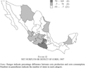
As corn imports are of no importance in ordinary years, domestic production and consumption are necessarily balanced. Therefore, if Kuntz's “pessimistic” view is accepted, we are confronted with a puzzle: the distribution of Mexican corn production across states—see Figure 12—clearly shows that some of them were net producers while other were net consumers in a normal year such as 1907.
51 On the assumption of no imports (17,787 metric tons or less than 1 percent of domestic production (Estadísticas Económicas del Porfiriato), we calculate the corn consumption for every state by multiplying population by 2.29 (resulting from dividing total domestic production among the Mexican population). The net surplus or deficit for every state equals consumption minus production. In Figure 11, they are shown in terms of percentage of the consumption needs.
NET SURPLUS OR DEFICIT OF CORN, 1907
A further result is also achieved by this exercise (see Figure 12). Some regional centers of production emerge (Chihuahua in the North; Tamaulipas in the North-East; Guanajuato, Mexico, Michoacan, etc. in the Center; Campeche in the Gulf). This picture is consistent with the idea that market integration, in such a vast, backward and geographically fragmented country as Porfirian Mexico, creates a center-periphery structure. The exercise also shows that the surplus produced in Chihuahua, Tamaulipas, and Campeche is not sufficient to cover the deficit of the surrounding and sparsely populated states. This situation contrasts with the massive surplus in a compact group of central, densely populated states. Therefore the integration of the corn market at a supraregional level is necessary to explain the surplus and deficit geography depicted in Figure 12.
CONCLUSIONS AND EXTENSIONS
Corn prices substantially differed across Mexican regional markets before 1885. However, between 1885 and 1908, the dispersion of corn prices decreased significantly. The least implausible explanation for price convergence is market integration. This process was not limited to some regions or agricultural products.
By applying panel data techniques, conditional convergence in corn prices is confirmed. Different groups of states present different steady states. Moreover, with only a few exceptions, after grouping steady states, a center-periphery geography emerges, in which most of “close-to-average” regions (i.e., Queretaro, Nuevo Leon, San Luis Potosi, Guerrero, Aguascalientes, etc.) occupy central—loosely defined—positions and “far-from-average” regions those in the periphery (i.e., Tepic, Campeche, Colima, Veracruz, Chiapas, Baja California, Sonora, etc.). The convergence speeds of Mexican regions are also far from being identical. Once again, a center-periphery spatial structure emerges clearly: convergence speed becomes slower almost continuously when moving from the central area (Hidalgo, Michoacan, Mexico, Morelos, and Tlaxcala) to the periphery (Campeche, Yucatán, Baja California, Sinaloa, and Sonora). However, as can be seen, the two geographies are not identical. We have also found evidence of a significant and positive influence of railroads on the convergence speeds of states. Conversely, no significant relationship between railroads and steady states has been found.
Although still incomplete on the eve of the Mexican Revolution, integration of regional corn markets substantially increased during the Porfiriato. Circa 1910, it was greater than in the years before the building of the railroad network. On the assumptions that increasing integration of corn market was impossible in the absence of some specialization at state or regional levels, and that specialization entails higher productivity, our results might lead to a more optimistic reconsideration of the growth of the nonexport agrarian sector during the Porfiriato.
Mexico does not turn out to be an exception in the international panorama of the late nineteenth and early twentieth centuries among those countries that took part in the economic globalization of the period. It would be interesting to examine the Mexican case from a comparative perspective.
An interesting extension would be to test whether or not the improvement brought about by railroads was complemented by other parallel improvements in the conventional means of transportation. It is our guess that railroads probably did not contribute to market integration only directly but also indirectly through the stimulation of complementary gains in the efficiency of traditional means of transportation.
The heterogeneity of the convergence process at the state level deserves further research. Differences in government regulation of the corn market across states and over time seems worth being explored. As to the heterogeneity in the steady states, a preliminary overview suggests that geography (altitude, climate, soils, distance to relevant locations, etc.) and supply and demand factors contribute to the explanation, at least partially.
Given the evidence available about corn, it is very likely that convergence of prices of other agricultural products should have been earlier and faster than generally thought so far. Testing this hypothesis within a similar analytical framework is an interesting task that might contribute to a full assessment of the general process of agricultural market integration in Porfirian Mexico. Analyzing the process of agricultural market integration during the revolutionary and postrevolutionary periods would provide not only an useful long-term perspective on this important issue but also some insights into the equally relevant determination of the economic consequences of the political instability prevailing in Mexico. This extension might or might not reinforce a certain revisionism, at least partially, of the traditional interpretation of the Revolution and its aftermath.
We are grateful to the following persons and institutions for their help and advice: David Rockefeller Center for Latin American Studies, Real Colegio Complutense en Harvard, John Coatsworth, Aurora Gómez, Enrique Llopis, Graciela Márquez, Teodosio Pérez, Jeffrey Williamson, participants in the seminars of CIDE (México) and Carlos III University (Getafe, Spain) and the editor and referees of JEH. We thank Gabriel Calderón for his assistance in research. Marrero also thanks the Fundación Ramón Areces and the Spanish Ministry of Education for the financial support through DGICYT grant no. BEC2003-03965.