1. Introduction
Philosophers of science have been exploring the concept of “species” for decades, but the related and arguably more important concept in ecology and evolution, “population,” has gone largely unexamined until very recently (e.g., Gannett Reference Gannett2003; Gildenhuys Reference Gildenhuys2009; Godfrey-Smith Reference Godfrey-Smith2009; Millstein Reference Ruse2009b, Reference Ruse, Bell, Futuyma, Eanes and Levinton2010; Bouchard Reference Bouchard2011). Elsewhere (Millstein Reference Ruse2009b, Reference Ruse, Bell, Futuyma, Eanes and Levinton2010) I defend a particular characterization of “population,” the causal interactionist population concept (CIPC), first through a demonstration that populations are individuals,Footnote 1 and second by showing how the CIPC illuminates case studies that include populations, metapopulations, and patchy populations of various types. In this paper I defend the CIPC in a different way: I show its usefulness in addressing a challenging conceptual and methodological issue in biology, namely, how to understand and deploy the concepts of “homogeneous environment” and “heterogeneous environment.” Thus, the first half of the paper is not on populations at all but rather on environment concepts; as a side benefit, I seek to further our understanding of these as well.
The structure of the paper is as follows. I begin with a historical case, “The Great Snail Debate” of the 1950s,Footnote 2 and show how during the course of that debate a disagreement over heterogeneous environments arose. I then consider whether Robert Brandon’s or Richard Levins’s concepts of “environment” can settle the disagreement; I argue that they cannot do so without further enhancement. I then suggest that we can deploy the concept of “population” to enhance our environment concepts and settle the disagreement. However, the common population-as-deme view is inadequate to the task; I show how the CIPC can succeed where the population-as-deme view fails. Last, I offer some concluding thoughts.
2. Heterogeneous Environments and “The Great Snail Debate” of the 1950s
The focus of the Great Snail Debate was the grove snail, Cepaea nemoralis, a land snail that is found throughout Europe and England. It is a highly polymorphic species and has been so since at least the Pleistocene, both in color (pink, brown, or yellow) and in the number of bands (having anywhere from zero to five visible bands). The snails live in numerous colonies of varying sizes, with some but very little migration between colonies.Footnote 3 Different colors and different numbers of bands predominate in different colonies; for example, the majority of snails in one colony might be yellow while the majority in a different colony might be pink. Disputants in the Great Snail Debate sought to determine which evolutionary processes accounted for the contemporary colony distributions.
There were two main camps involved in the Great Snail Debate. The first camp, Arthur J. Cain and Philip Sheppard, was studying the snails in England. They argued that the snail distributions were primarily due to selection, with little or no role for random drift. The second camp, Maxime Lamotte, was studying the snails in France. He agreed with Cain and Sheppard that the snail distributions were partially due to selection; however, he argued that there was in fact a substantial role for drift. Importantly, however, both camps agreed that there were correlations between snail colors and habitat backgrounds due to visual selection by predator; thrushes would find it harder to spot snails whose colors were similar to that of their background, giving the camouflaged snails an advantage in those environments.
In the course of the debate, Cain and Sheppard criticized Lamotte’s inclusion of large colonies in his studies:
Because backgrounds vary considerably over small distances, and the larger colonies will tend to be spread over larger areas and therefore over more types of background than the smaller ones,Footnote 4 it is to be expected that large colonies will tend to be more alike, since the diverse effects of selection in different parts of each colony will tend to cancel out when the colony is considered as a whole, and in any case will be reduced to a certain extent by gene flow. Small colonies will tend to be on more homogeneous backgrounds, and will therefore become more diverse by selection. (1954, 110; emphasis added)
In this passage, Cain and Sheppard seem to be suggesting that selection is occurring within microhabitats and that by examining the whole (heterogeneous) environment of a particular colony, one would miss these more localized selection processes. Indeed, Cain and Sheppard stated that they were “avoiding those [localities] where there is a mixture of types of vegetable formations” (Reference Cain and Sheppard1954, 98).
Thus, Cain and Sheppard seem to have thought that natural selection occurs in homogeneous environments, so that if a colony of snails was in a heterogeneous area, the data from these colonies should not be included because the effects of the selective processes in homogeneous microhabitats would average out. Lamotte, however, disagreed; he seems to have thought that evolutionary processes could occur across heterogeneous environments, and so he thought that data from colonies living in heterogeneous areas ought to be included. Homogenous environments, Lamotte asserted, were rare in France; he did his “best to study the populations in all possible environments” (Reference Lamotte1959, 70–72).
But what does it mean for an environment to be heterogeneous or homogenous? And which is the relevant environment for evolutionary processes?
3. Environment Concepts
3.1. Brandon’s Concepts of “Environment”
Robert Brandon has argued for the importance of understanding concepts of environment; as he notes in his coauthored paper with Antonovics and Ellstrand, “for the theory of natural selection to have explanatory power with regard to how adaptations originate, the concept of environment is as important as that of fitness” (Antonovics, Ellstrand, and Brandon Reference Antonovics, Ellstrand, Brandon, Gottlieb and Jain1988, 280). According to Brandon (Reference Brandon1990), we need to distinguish between three different concepts of environment:
1. External environment—the sum total of biotic and abiotic factors external to the organisms in question. Some of these factors may not affect organisms’ fitness or relative fitness, so an external environment can look heterogeneous but be homogeneous from the organisms’ point of view, which leads to the second concept of environment.
2. Ecological environment—consists of only those features of the external environment that affect the fitness of a given genotype; organisms “define” their environments. These are homogeneous when fitness values remain relatively constant across the area.
3. Selective environment—consists of only those features of the external environment that affect the relative fitnesses of multiple genotypes in an area. These are homogeneous when the relative fitness values remain relatively constant across the area (at a minimum, homogeneity requires that the ordinal relation of genotypes not change across the area).
Brandon further suggests that organisms that are mobile enough to move between environmental patches are in a homogeneous selective environment: “Moths fly around and land on many different trees. Their probability of being devoured by a bird depends on the match, or lack thereof, of their color and the statistical average color of the background that they create by their behavior. Thus if the two tree types are distributed randomly about the woods and both types of moths show no behavioral preference for one type of tree over the other, then the woods in question are selectively homogeneous” (2005, 166).
Moreover, Antonovics et al. argue that, understood properly, selection occurs in homogeneous selective environments:Footnote 5
If we grew one plant on good soil, and another on poor soil, the one on good soil would probably survive better, grow larger, and have more seed. Although we might be tempted to say one plant had a greater ‘fitness’ than the other, we are in this case referring to properties of the environment rather than to properties of the phenotypes of those plants which would explain their differential success. . . . In other words for the theory of natural selection to have explanatory power, we must compare the fitness of different phenotypes in identical environments. Conversely, two environments can be thought of as homogeneous (with regard to selection) if their effect on the relative fitness of phenotypes is the same. It is within such selectively homogeneous environments that differential fitness is the result of properties of the organism and within which the theory of natural selection therefore has explanatory power. (1988, 280; emphasis added)
If Cain and Sheppard held views similar to these, and if they thought that the snails were not very mobile (i.e., not mobile enough to move between environmental patches in some areas), then they would have thought that in some cases the snails were not in homogeneous selective environments. Thus (again assuming that Cain and Sheppard’s views were similar to Brandon’s), they would have refused to consider data from colonies in heterogeneous environments, as they indeed did.
3.2. Levins’s Concepts of “Environment”
Although many philosophers are familiar with Brandon’s concepts of environment, those of Richard Levins (Reference Levins1968) are better known among biologists. Levins classifies environments in evolutionary contexts somewhat differently than Brandon; instead of two categories of selective environment (homogeneous and heterogeneous), there are three:
1. Homogeneous environment—organisms spend their lives in a uniform environment.
2. Fine-grained heterogeneous environment—organisms disperse freely among many patches (in space or time) during the course of their lifetime.
3. Coarse-grained heterogeneous environment—organisms spend their lives in one patch.
Note that intermediates between the extremes of “fine-grained” and “coarse-grained” environments are possible, that is, organisms may spend their lives in more than one patch yet not disperse freely enough so that they experience them with a frequency equivalent to that of the environment. However, in many cases the extremes are reasonable approximations, so in what follows I ignore the possibility of intermediates.
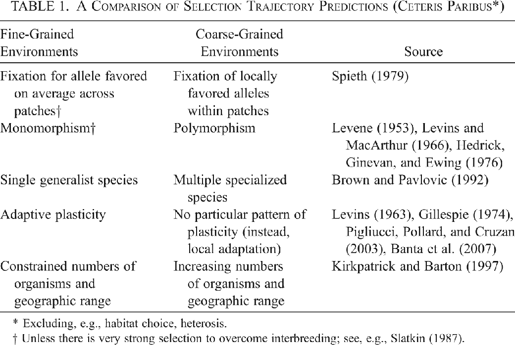
The category of fine-grained heterogeneous environments marks a difference between Brandon’s typology and Levins’s; recall that such an environment would count as homogeneous for Brandon. That difference is important because certain phenomena may be expected in a fine-grained heterogeneous environment that would not necessarily be expected in a Levins-sense homogeneous one. For example, selection for adaptive plasticity is more likely in a fine-grained environment than it is in one that is Levins-sense homogenous; organisms in fine-grained environments are also more likely to experience constrained geographic ranges if interbreeding inhibits adaptation to environmental extremes (see table 1). Therefore, the concepts of “fine-grained heterogeneous environment” and “homogeneous environment” should not be collapsed. Levins’s typology is superior to that of Brandon’s in that respect.

| Fine-Grained Environments | Coarse-Grained Environments | Source |
|---|---|---|
| Fixation for allele favored on average across patches† | Fixation of locally favored alleles within patches | Spieth (Reference Spieth1979) |
| Monomorphism† | Polymorphism | Levene (Reference Levene1953), Levins and MacArthur (Reference Levins and MacArthur1966), Hedrick, Ginevan, and Ewing (Reference Hedrick, Ginevan and Ewing1976) |
| Single generalist species | Multiple specialized species | Brown and Pavlovic (Reference Brown and Pavlovic1992) |
| Adaptive plasticity | No particular pattern of plasticity (instead, local adaptation) | Levins (Reference Levins1963), Gillespie (Reference Gillespie1974), Pigliucci, Pollard, and Cruzan (Reference Pigliucci, Pollard and Cruzan2003), Banta et al. (Reference Banta, Dole, Cruzan and Pigliucci2007) |
| Constrained numbers of organisms and geographic range | Increasing numbers of organisms and geographic range | Kirkpatrick and Barton (Reference Kirkpatrick and Barton1997) |
* Excluding, e.g., habitat choice, heterosis.
† Unless there is very strong selection to overcome interbreeding; see, e.g., Slatkin (Reference Slatkin1987).
However, Brandon is certainly right to emphasize that organisms determine the nature of the selective environment. (Not that Levins would likely disagree; after all, the distinction between fine grained and coarse grained is itself organism centered). Thus, the two typologies might be profitably (but tentatively—I make further refinements below) combined as follows:
1. Homogeneous selective environment—consists of only those features of the external environment that cause the relative fitnesses of multiple genotypes in an area to remain relatively constant across the area.
2. Fine-grained heterogeneous selective environment—consists of only those features of the external environment that cause the relative fitnesses of multiple genotypes in an area to vary across the area, where organisms disperse freely among many patches (in space or time) during the course of their lifetime.
3. Coarse-grained heterogeneous selective environment—consists of only those features of the external environment that cause the relative fitnesses of multiple genotypes in an area to vary across the area, where organisms spend their lives in one patch.
A couple of clarifications here: First, the term “selective environment” should not be taken to exclude other evolutionary processes from occurring in the same area, drift in particular. Second, speaking of a heterogeneous selective environment might seem to be begging the question against Brandon. In section 4.2 I explain why such a locution is sensible and desirable.
3.3. Incompleteness of Environment Concepts
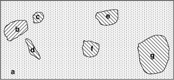
Even by combining the best elements of Levins’s and Brandon’s concepts, we cannot settle the question of which environments to consider in the snail studies because in many cases it will be unclear when we have homogeneous environments and when we have heterogeneous environments. To see this, consider the region shown in figure 1, consisting of three patch types relevant to the fitness of the organisms (e.g., pink, brown, and yellow snails distributed across pinkish, brownish, and yellow-greenish backgrounds). Suppose that the snails only regularly move between some patches: between a, b, c, and d; between e, a, and f; and within (but not outside of) g. Now consider three ways of drawing area boundaries:
1. Around each patch individually, so that there are seven areas.
Figure 1.Patchy region. In the figure, a is one patch type (e.g., brownish background), b is a second patch type (e.g., pinkish background), and c, d, e, f, and g are a third patch type (e.g., yellow-greenish background).

2. Around the entire region depicted, so that there is one area.
3. Around b, c, and d, including some of a; around e and f, including some of a; and around g, including some of a.

If the boundaries are drawn the first way, there are seven homogeneous environments. If the boundaries are drawn the second way, there is one coarse-grained heterogeneous environment. If the boundaries are drawn the third way, there are three heterogeneous environments, two of which are fine grained and one of which is coarse grained.
This variability in classifying environments as homogenous, coarse-grained heterogeneous, or fine-grained heterogeneous arises because both Levins and Brandon are silent on the question of how one delineates the boundaries of a selective environment. Thus, the Brandon and Levins environment concepts are incomplete. They cannot help to settle disputes (like the one between Lamotte and the team of Cain and Sheppard) over which areas to include in one’s data set because they are not powerful enough to determine which areas are heterogeneous and in what way. Yet, whether the environments are fine grained or coarse grained matters; table 1 compares the predictions of a fine-grained heterogeneous environment with those of a coarse-grained one.
Consider, for example, the first row of table 1. If organisms are frequently changing selectively relevant patches in space or time (a fine-grained environment), then even though a trait might be advantageous for an organism in one patch (e.g., a yellow snail in a yellow-greenish background), that same trait might be disadvantageous in another patch (e.g., a yellow snail in a pinkish background). Such a trait might therefore be selected against. The trait that would do best, while perhaps not particularly advantageous in any of the patches, is one that is the most favorable on average (or, alternatively, as the fourth row of the table indicates, an adaptively plastic trait). It is fairly straightforward to see how this might lead to a monomorphic population (second row) with no particular predisposition to speciate (third row); moreover, organisms might have difficulty expanding their numbers outside of the range if the edges of the range are much different from the habitat in the interior (fifth row). On the other hand, if organisms are spending their lives in one patch (a coarse-grained environment), they can more easily adapt to their particular patch, perhaps leading to fixation of the favored allele (first row) and thus polymorphism, since there are different adaptations within the species (second row). Over time, these polymorphisms might become separate species (third row); however, there is no particular expectation of adaptive plasticity (fourth row) or reason to think that organisms are limited in their numbers or geographic range (fifth row).
In short, table 1 shows that if boundaries are drawn any way that one chooses, one risks making the wrong predictions because the location of an environment’s boundaries affects whether the environment is fine grained or coarse grained (as the discussion of fig. 1 shows). Thus, to deploy our environment concepts in a way that preserves our ability to make accurate predictions, we need a principled way to draw the boundaries.
4. The Population Concept Completes the Environment Concepts
My suggestion, consistent with the standard view that it is populations that undergo evolution, is that populations dictate the boundaries of the selective environment.Footnote 6 More specifically, the boundaries of the environment would be delineated by the fullest extent of the spatial location of the population. To illustrate, consider figure 1 again. If there were separate populations in each of the seven background patches, then there would be seven separate homogeneous environments. On the other hand, if populations were to occur in more than one background patch, then the environment(s) would be heterogeneous; then, based on the frequency of organisms changing patches in space and time, we could determine whether a given heterogeneous environment is fine grained or coarse grained.
Here are four advantages of recognizing that populations bound environments (more later). First, I think that this recognition is implicitly assumed in the widely used Levins typology of environments.Footnote 7 Second, it follows Brandon’s reasonable intuition that environments should be understood relative to the organisms that inhabit them. Third, it avoids the problems of an “anything goes” boundary solution, which would not be consistent with the different predictions in different types of environments shown in table 1. And fourth, it respects the types of predictions of homogeneous versus fine-grained versus coarse-grained environments; note that these were mostly population-level predictions (polymorphism, fixation, etc.) and that the predictions reflect the “common fate” experienced by organisms of the same population.
Thus, we need a population concept to delineate the environment in which organisms are evolving. But which population concept?
4.1. Population-as-Deme
The most common answer among population geneticists is that populations are demes, that is, groups of actively interbreeding organisms of the same species. If we take my suggestion that populations delineate environments together with the population-as-deme view, then the boundaries of the environment would be delineated by the fullest extent of the spatial location of the interbreeding organisms.
However, the population-as-deme view is problematic. To see why, suppose that a population sensu deme is spread across a heterogeneous environment with two patches. Suppose further that, over time, local adaptation occurs in each of the habitat patches and organisms in the different patches differentiate enough that we would call them different species on some reasonable species concept. (Species that exhibit configurations similar to this include threespine stickleback fish, metal-tolerant grasses, and hawthorn and apple maggots [Rhagoletis pomonella].) Under this scenario, there could be significant differentiation between organisms, but unless there were a significant change in breeding patterns, there would still only be one population according to the population-as-deme view. Thus, breeding-related differentiation would count (e.g., habitat choice, assortative mating), but non-breeding-related differentiation would not (e.g., differential adaptation), even though both types of differentiation can lead to speciation.
This seems arbitrary and incomplete. Arguably, one aspect of being a population is as a possible precursor to a new species, yet some precursors are not recognized (while others are). The significant differentiation prior to speciation ought to be recognized conceptually, especially since differential adaptation with linkage can limit gene flow. The failure to do so is a flaw of the population-as-deme view.
4.2. The Causal Interactionist Population Concept
The CIPC is an alternative to the population-as-deme view. Details of the view can be found elsewhere (Millstein Reference Ruse2009b, Reference Ruse, Bell, Futuyma, Eanes and Levinton2010); here I summarize briefly. The CIPC characterizes populations in ecological and evolutionary contexts as consisting of at least two conspecific organisms that, over the course of a generation, are actually engaged in survival or reproductive interactions, or both.Footnote 8 The boundaries of the population are the largest grouping for which the rates of interaction are much higher within the grouping than outside.Footnote 9 Both reproductive and survival interactions should be understood broadly; relevant interactions include both unsuccessful and successful matings (interbreeding), offspring rearing, competition for limited resources, and cooperative activities.
Recall the scenario where there was local adaptation within two patches with widespread interbreeding across patches. Now suppose that in addition to reproductive interactions within and between organisms in patches, there were significant survival interaction rates within (but not between) patches. Since the rates of causal interactions within patches are significantly greater than the rates of causal interactions more generally, on the CIPC there are two populations (which may later become two species). Thus, there are two homogeneous evolutionary environments whose boundaries are delineated by the spatial range of the causal interactions of the two populations. Since there are some interactions across the two populations, they form a metapopulation across a heterogeneous environment (probably, but not necessarily, coarse grained, if interactions are a good proxy for the movement of organisms through space and time).Footnote 10 Therefore, the CIPC, unlike the population-as-deme view, preserves the idea that splitting into populations precedes splitting into species. On the other hand, according to the CIPC, if the rates of causal interactions within patches were not significantly greater than the rates of causal interactions more generally, then there would be only one population evolving in a heterogeneous environment (probably, but not necessarily, fine grained—again, it would depend on the movement of organisms through space and time).
Note that using the CIPC (or the population-as-deme view, for that matter) to delineate the boundaries of the selective environment entails that selection can occur across a heterogeneous environment, contra the view of Brandon and others that selection should be understood within homogeneous environments only. Indeed, the authors cited in table 1 suggest that thinking of selection occurring across heterogeneous environments is widespread. But is it legitimate? Recall that in Brandon’s view, fine-grained heterogeneous environments are considered homogenous, so it is only the coarse-grained ones that are controversial. Brandon handles the latter type of case by calling selection within a selectively homogeneous environment “simple natural selection,” whereas selection in coarse-grained environments is “compound natural selection”—“a process consisting of natural selection within environments and distribution into environments” (1990, 73). For example, suppose that the pollen and seeds of two plant genotypes are randomly distributed across two habitat patches, one where the soil contains heavy metals and one where it does not.Footnote 11 On Brandon’s view, the distribution forms the first part of the process of compound natural selection. Then suppose that there is selection within each of the environmental patches, with one genotype being favored in the soil that contains heavy metals and the other genotype being favored in the soil that does not contain heavy metals. The selection within these two environments is the second part of the process, according to Brandon. Thus, although Brandon does speak of selection within heterogeneous environments, in truth on his account the selection part of compound natural selection is occurring within homogeneous selective environments; only the distribution occurs across heterogeneous environments.
However, there are reasons to think that selection itself can occur across heterogeneous environments, as using the CIPC as an environment delineator would imply. Consider (as Brandon would readily acknowledge) that there are reproductive interactions occurring across the habitat patches. In addition, there are likely to be survival interactions occurring across patches, particularly between plants that are near the borderline between the two patches; for example, the plants on different sides of the patch will probably be competing for water, for nutrients in the soil, for light, and for root space. Even if two plants on different sides of the border are not competing directly, they may be affected by the competition between the plants that are near the border, meaning that because of those near-border competitions there is more or less water available for them, more or fewer nutrients, etc. These sorts of survival interactions—examples of Darwin’s “struggle for existence”—are part of the process of natural selection. It thus does not make sense, in situations such as those described here, to say that there are two separate selection processes when in fact all of the organisms in both patches are engaged in a struggle for existence and in reproductive interactions (also part of natural selection) with one another. Of course, it is also possible that there are cases where few or no interactions occur across patches, or where those interactions were very much fewer than the interactions within the patches; in those cases, there would be two separate selection processes going on in two separate environments. These considerations vindicate the CIPC approach to environment delineation.Footnote 12
Furthermore, unlike the population-as-deme view, the CIPC helps us understand debates like the Great Snail Debate. Recall that Cain and Sheppard disagreed with Lamotte over the relevant type of environment for evolutionary processes. Cain and Sheppard thought that each individual patch within the area is its own (homogenous) environment and that these should be studied separately, whereas Lamotte thought that one heterogeneous area as a whole characterizes the environment. If the rates of interactions within patches were much higher than the rates of interactions between patches, then in a sense both camps were right. Cain and Sheppard’s view would let us study the dynamics of the populations, while Lamotte’s view would let us study the dynamics of the metapopulation. However, if the rates of interactions were more or less consistent across patches, then Lamotte was right: we should study a colony’s entire heterogeneous environment.
5. Conclusions
I have argued that we ought to characterize our environment concepts as described in section 3.2 with the CIPC-based delineations specified in section 4.2. When trying to understand the evolution of organisms spread over heterogeneous areas, the CIPC directs us to (1) pay attention to the interactions of organisms across the landscape; (2) identify the fullest extent of the densest pockets of survival and reproductive interactions, that is, the populations; and (3) delineate the environments based on the geographic range of the populations. Once that is done, we can determine whether the environments are homogeneous or heterogeneous, and if heterogeneous, whether coarse grained or fine grained (based on the dispersal abilities of the organisms). We can then determine the appropriate models to apply to our study populations.
The case for a population concept in evolutionary and ecological contexts, and the CIPC more specifically, now rests on (1) a demonstration that populations are individuals (Millstein Reference Ruse2009b), (2) an illustration of how the CIPC illuminates a variety of different population structures (continuous populations, metapopulations, patchy populations, etc.) for a variety of species (Millstein Reference Ruse, Bell, Futuyma, Eanes and Levinton2010),Footnote 13 and (3) an argument that the CIPC is required for understanding and deploying concepts of homogeneous and heterogeneous environment (this paper). Furthermore, the discussion above hints at other roles for the CIPC to play. Since selection in heterogeneous environments is thought to be one mechanism through which sympatric speciation can occur, the CIPC may help clarify this somewhat-controversial process by elucidating the separation of populations prior to the separation of species. In addition, since the 1950s many other processes have been proposed to explain the distributions of the Cepaea nemoralis populations, including repeated extinction and recolonization of habitat patches (Cameron and Pannett Reference Cameron and Pannett1985; Cameron Reference Cameron2001), founder effects (Cameron and Dillon Reference Cameron and Dillon1984), and rare, long-distance migrations (Davison Reference Davison2000); a robust population concept like the CIPC would seem to be relevant to each of these phenomena. However, these are topics for another day.