4.1. The diffusive and linear-growth regimes

The diffusive and linear-growth regimes are analysed together because they have similar length and time scales. The dissolution flux $F$ decays with $t^{1/2}$ in the diffusive regime (Ennis-King et al. Reference Ennis-King, Preston and Paterson2005; Slim Reference Slim2014). When $F$ and $t$ are normalized with the diffusive scales $u_I$ and $l_I$, their relation can be expressed theoretically as

(4.1)\begin{equation} F/u_I=1/\sqrt{{\rm \pi} t/t_I}. \end{equation}

Equation (4.1) indicates that the relationship between $F/u_I$ and $t/t_I$ is independent of $Ra$, $Sc$, $H/s$ and the pore-scale geometry in the diffusive regime (the dimensional dissolution flux $F$ still depends on these dimensionless parameters). This is confirmed by figure 4(a), where $F/u_I$ for different values of $Ra$, $Sc$ and $H/s$ are compared. However, the collapsed profiles deviate from the theoretical equation (4.1). The reason for this is that the effective diffusivity $D_e$, which is used to calculate $u_I$ and $t_I$, is obtained when the diffusion in the porous medium reaches the equilibrium state. However, this equilibrium state is not reached when the diffusion starts. The effective diffusivity should be close to the molecular diffusion $D$ before the diffusion is affected by the porous elements. If $D$ is used instead of $D_e$ to calculate the diffusive scales, then the modified velocity and time scales become $u_I/\gamma _m$ and $\gamma _m t_I$, respectively. Normalized with the modified diffusive scales, the profiles become identical to those of the theoretical equation in the early stage of diffusion; see figure 4(b). The pore scale starts to affect the diffusion when the solute reaches the porous elements. As a result, $\gamma _m F/u_I$ becomes lower than the theoretical solution. As an approximation, $u_I$ and $t_I$ (instead of $u_I/\gamma _m$ and $\gamma _m t_I$) are still used in (4.1) to calculate the dissolution flux in the diffusive regime. In addition, figure 4 shows that the Schmidt number has very little effect on convection when $Sc>250$.

Figure 4.

Dimensionless dissolution flux versus dimensionless time; $Sc$, $Ra$ and $H/s$ are varied. (a) The diffusive scales $u_I$ and $t_I$ are used to normalize $F$ and $t$. (b) The modified diffusive scales $u_I/\gamma _m$ and $\gamma _m t_I$ are used to normalize $F$ and $t$.

Figure 5 shows the time evolution of $\gamma _m F/u_I$ for typical cases of different pore-scale geometries. Again, the DNS results are almost identical to the theoretical solution in the early stage of diffusion. The results from the different pore-scale geometries deviate after the porous matrix affects the diffusion; they also deviate from the theoretical solution. Note that $\gamma _m F/u_I$ for case G3R1S1H1 (S15) is even higher than the analytical solution during the period $10 \le t/(\gamma _m t_I) \le 40$. This indicates the significant pore-scale effect in the diffusive regime.

Figure 5.

Dimensionless dissolution flux versus dimensionless time. The pore-scale geometry is varied. The modified diffusive scales $u_I/\gamma _m$ and $\gamma _m t_I$ are used to normalize $F$ and $t$.

As the solute accumulates near the upper boundary, some perturbations appear in the concentration field, leading to the linear-growth regime. The linear-growth regime cannot be evidently identified in the $F\unicode{x2013}t$ profiles. However, it can be visualized in the concentration field; see figure 6. A slight perturbation can be found at location $A$ at $t/t_I=10.2$ in figure 6(a), where the solute is transported more slowly than in the neighbouring REVs. This perturbation expands and amplifies as the boundary layer reaches the second row of the porous elements adjacent to the wall. Figure 6(b) shows that the solute is transported slower at location $A$ and faster at location $B$. This leads to instability of the flow and the onset of convection.

Figure 6.

Solute concentration fields during the linear-growth regime, case G1R1S1H1 (S1), for (a) $t/t_I=10.2$, (b) $t/t_I=12$. The light curves indicate the isosurfaces of $\tilde {c}=0.01$.

4.2. The onset of convection and the flux-growth regime

The thickness of the solute boundary layer increases with time in the diffusive regime. Convection begins when the porous matrix can no longer hold the heavy fluid in the boundary layer. Figure 7 shows the time evolution of the concentration field at the interface of the first and second REVs near the upper boundary ($x_2=-s$), which is indicated in figure 6(a). The results of $\tilde {c}(x_1, t)$ are shown in a two-dimensional colour map. The horizontal coordinate $x_1$ is normalized with the pore size $s$, so that $x_1/s$ ranges from 0 to 100 in case G1R1S1H2 (S6), which has 100 REVs in the horizontal ($x_1$) direction. The onset of convection in this test case occurs at $t_{oc}/t_I=22.4$. Weak vertical stripes with spacing $s$ can be found before the onset of convection. These stripes are caused by the different diffusion velocities in the pores. Perturbations with low wavenumbers $\kappa ={\rm \pi} L/l=7{\rm \pi}$ and $3.5{\rm \pi}$, where $l$ is the wavelength, can be observed before the onset of convection. They correspond to the wavelengths $l=L/7$ and $2L/7$. The low-wavenumber fluctuation is enhanced after the onset of convection. In addition, strong high-wavenumber fluctuations are also observed, represented by the vertical stripes with spacing $2s$.

Figure 7.

Time evolution of the concentration field at the interface between the first and second REV rows ($x_2=-s$) near the onset of convection ($20\le t/t_I \le 28.5$), case G1R1S1H2 (S6).

The high-wavenumber stripes correspond to the convective figures (original plumes) generated after the onset of convection. Figure 8 confirms that the spacing of the convective figures is approximately $2s$. The convection causes the fast transport of the solute in the vertical ($x_2$) direction in the flux-growth regime, while the dispersion in the horizontal direction has no significant effect. Note that the high-wavenumber original plumes cannot be captured in a macroscopic simulation without modelling the pore-scale motions.

Figure 8.

Solute concentration field during the flux-growth regime, case G1R1S1H1 (S1).

The dimensional analysis in § 2.2 shows that the dissolution process is determined by the dimensionless parameters $Ra_K$, $Da$, $Sc$ and the pore-scale geometry (characterized by $\phi$ and $\gamma _m$). Neglecting the effect of $Sc$ and considering a specified pore-scale geometry, it can be found that the dissolution process is determined only by $Ra_K$ before the plumes reach the bottom wall. Considering the relationship $Ra_K=(t_I/t_{II})^{1/2}$, it can be expected that the onset time of convection $t_{oc}$ is related only to the diffusive and convective time scales $t_I$ and $t_{II}$. The relationship is expressed as

(4.2)\begin{equation} t_{oc}=A_1 t_I^{1-\alpha_1} t_{II}^{\alpha_1}, \end{equation}

where $A_1$ and $\alpha _1$ are the scaling coefficients. Considering $Ra_K=({t_I}/t_{II})^{1/2}$, the dimensionless onset time $t_{oc}/t_I$ has the scaling $t_{oc}/t_I \sim Ra_K^{-2\alpha _1}$. According to (4.1), the dissolution flux at the onset of convection has the scaling $F_{oc}/u_I \sim Ra_K^{\alpha _1}$. In the constant-flux regime, the constant flux $F_{cf}$ has the scaling $F_{cf} / u_I \sim Ra_K$, which is equivalent to $F_{cf} / u_{II} = const$. For low $Ra_K$, $\alpha _1$ should have the value $\alpha _1=1$ to ensure that $F_{oc}/u_I$ varies with $Ra_K$ at the same rate as $F_{cf}/u_I$. This is in accordance with the study by Riaz et al. (Reference Riaz, Hesse, Tchelepi and Orr2006), who propose the onset time of convection to be $t_{oc}=146t_{II}$, and the study by Slim & Ramakrishnan (Reference Slim and Ramakrishnan2010), who propose the earliest possible onset time to be $t_{oc}=47.9t_{II}$.

Figure 9 shows the dimensionless onset time of convection $t_{oc} / t_I$ for different values of $Ra_K$. In addition to the cases listed in table 2, some other DNS cases have been calculated to study the onset time of convection for small pore-scale Rayleigh numbers (up to $Ra_K =0.01$). It can be observed that $t_{oc}$ from the DNS results is higher than the theoretical values suggested by Riaz et al. (Reference Riaz, Hesse, Tchelepi and Orr2006) and Slim & Ramakrishnan (Reference Slim and Ramakrishnan2010). This difference is due to the fact that $t_{oc}$ is defined as the start time of the flux-growth regime in this study, whereas the correlation in Slim & Ramakrishnan (Reference Slim and Ramakrishnan2010) is proposed for the earliest possible onset time (the start time of the linear-growth regime). The DNS results show that $t_{oc}$ is very sensitive to perturbations in the flow field at large $Ra_K$. However, it is still possible to estimate $t_{oc}$ from the DNS results at low $Ra_K$ ($Ra_K \le 1$), which gives the scaling coefficient $\alpha _1=1$ in (4.2). The present DNS results show the same scaling coefficient $\alpha _1$ as those of Riaz et al. (Reference Riaz, Hesse, Tchelepi and Orr2006) and Slim & Ramakrishnan (Reference Slim and Ramakrishnan2010). The other coefficient $A_1$ increases from 1200 to 3000 as the porosity increases from $0.32$ to $0.56$. Note that the DNS results show that $\alpha _1$ is less than 1 at large $Ra_K$. Therefore, (4.2) with the given coefficients may under-predict the onset time of convection at large $Ra_K$.

Figure 9.

Dimensionless time for the onset of convection $t_{oc}/t_I$. The DNS results are compared with the correlation equations.

The convection enters the flux-growth regime after the onset of the convection. In this regime, the dissolution flux grows rapidly until it reaches its maximum value $F_{fg}$. Figure 10 shows that the dimensionless period of the flux-growth regime $\Delta t_{fg}/t_I$ increases with increasing $t_{oc}/t_I$. Using a linear approximation, the relationship between $\Delta t_{fg}$ and $t_{oc}$ is expressed as

(4.3)\begin{equation} \Delta t_{fg}=A_2t_{oc}. \end{equation}

The scaling coefficient $A_2$ is close to $0.5$ at small $Ra_K$.

Figure 10.

Time evolution of the dimensionless concentration flux at the upper boundary $F/u_I$, where $Ra$ and $H/s$ are varied: (a) geometry G1 (square elements with $\phi =0.56$); (b) geometries G2 (square elements with $\phi =0.36$) and G3 (circular elements with $\phi =0.32$).

To ensure that $F_{fg}/u_I$ varies at the same rate as $F_{cf}/u_I$ with $Ra_K$, there should be the scaling law

(4.4)\begin{equation} F_{fg} / {u_I} = A_3 Ra_K, \end{equation}

which is equivalent to $F_{fg} / u_{II} = A_3$. Considering that the time to reach the maximum flux $t_{fg}$ has the scaling law $t_{fg} / {t_I} \sim Ra_K^{-2\alpha _1}$, $F_{fg} / {u_I}$ should also have the scaling law

(4.5)\begin{equation} F_{fg} / {u_I} \sim \left(t_{fg} / t_I\right)^{{-}1/(2\alpha_1)}. \end{equation}

This means that $F_{fg} / {u_I}$ decreases with the scaling $(t_{fg} / t_I)^{-1/2}$ for small $Ra_K$, while it decreases faster for large $Ra_K$. This is confirmed by the DNS results in figure 10, which shows that $F_{fg} / {u_I}$ decreases with the scaling $(t_{fg} / t_I)^{-0.7}$ for large $Ra_K$. The DNS show that the scaling coefficient $A_3$ depends on the pore-scale geometry. It takes value $0.04$ for geometry G1, and $0.026$ for geometries G2 and G3.

Using a linear approximation, the dimensionless dissolution flux in the flux-growth regime can be calculated as

(4.6)\begin{equation} F = F_{oc}+(t-t_{oc})\,\frac{F_{fg}-F_{oc}}{\Delta t_{fg}}. \end{equation}

The onset dissolution flux $F_{oc}$ can be calculated using the diffusion equation (4.1) with $t=t_{oc}$.

4.3. The merging re-initiation regime

The dissolution flux decreases after reaching its maximum value, and the convection thereafter enters the merging re-initiation regime. Figure 11 shows the time evolution of the concentration field on the line $x_2=-s$ during the merging re-initiation regime. Typical events of re-initiation and merging are indicated by ${R_i}$ and ${M_i}$ in the figure, where the subscript ${i}$ denotes the index of an event. It can be seen that the plume merging and re-initiation occur in the same period; see ${R_1}$ and ${M_1}$ in figure 11. Therefore, in this study, the merging and re-initiation regimes are combined into the merging re-initiation regime. The original plumes that have spacing $2s$ are identified by the straight vertical stripes in the figure. These vertical stripes decay rapidly due to the pore-scale dispersion. Both symmetric (${R_1}$, ${R_2}$ and ${R_3}$) and asymmetric (${R_4}$) structures of plume re-initiation can be found in the figure. This means that the new plumes can spread in both ($x_1$ and $x_2$) directions or in a single direction. Dispersion plays an important role in plume dynamics. Horizontal dispersion causes the original plumes (convective figures) to merge (${M}_1$ and ${M}_2$). It also causes an original plume to merge with a new plume (${M}_3$).

Figure 11.

Time evolution of the concentration field at the interface between the first and second REV rows ($x_2=-s$) near the upper boundary during the merging re-initiation regime ($28.5\le t/t_I \le 71.3$), case G1R1S1H2 (S6). Typical events of re-initiation (${R_1}$–${R_4}$) and merging (${M_1}$–${M_3}$) are indicated.

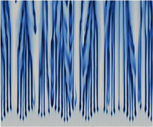
Figure 12 shows the instantaneous REV-averaged concentration fields in the merging re-initiation regime for the cases with different scale ratios and Rayleigh numbers. The convective fingers extended in the vertical direction can be clearly observed in all cases. The plume merging and re-initiation cannot be clearly observed since they occur only near the upper boundary. Figures 12(a–c) have the same Rayleigh number $Ra=20\,000$. As the scale ratio $H/s$ increases from 50 to 200, the corresponding $Ra_K$ value decreases from 23.7 to 6. Discontinuity of the convective fingers is observed in figure 12(c) ($Ra_K=6$). This phenomenon is due to the intermittent eruption of the convection (not only at the top boundary, but also near the porous elements). When the solute accumulates in a REV, the eruption of convection occurs when the porous matrix can no longer hold the heavy fluid. This is similar to the onset of convection at the upper boundary. It can be seen in figure 9 that the onset time of convection has significant uncertainties at high $\phi$ and $Ra_K$ values. These uncertainties are expected to cause the discontinuity of the plumes. At low $Ra_K$ (figure 12e), strong plume instability is still observed near the upper boundary, causing the plume re-initiation. Compared to high-$Ra_K$ convection, the diffusion has a more significant effect at low $Ra_K$. This is in accordance with the study in Gasow et al. (Reference Gasow, Kuznetsov, Avila and Jin2021), which suggests that the macroscopic diffusion cannot be neglected at low Darcy numbers.

Figure 12.

The REV-averaged solute concentration $\langle \tilde {c}\rangle$ fields during the merging re-initiation regime: (a) $Ra=20\,000$, $H/s=50$, case G1R1S1H2 (S6); (b) $Ra=20\,000$, $H/s=100$, case G1R1S1H3 (S7); (c) $Ra=20\,000$, $H/s=200$, case G1R1S1H4 (S8); (d) $Ra=80\,000$, $H/s=400$, case G1R1S1H5 (S9); (e) $Ra=1600$, $H/s=200$, case G2R4S1H3 (S14). Part of the computational domain near the upper boundary is shown.

Figure 13 shows the power spectra of the dimensionless concentration $E_c$ on the line $x_2=-s$ at typical times. Some low-wavenumber fluctuations ($0.05 \le \kappa /\kappa _p \le 0.07$) can be found in the merging re-initiation regime (the solid lines), where $\kappa _p={\rm \pi} L/s$ is the wavenumber for the pore size $s$. However, the high-wavenumber fluctuations ($0.44\le \kappa /\kappa _p \le 0.56$) are dominant at this time. These high-wavenumber fluctuations decay rapidly, while the low-wavenumber fluctuations gradually dominate. Note that some high-wavenumber fluctuations can still be observed even after the merging re-initiation regime.

Figure 13.

Power spectra of the solute concentration $\tilde {c}$ at the interface between the first and second REV rows ($x_2=-s$) for cases with different pore-scale geometries: (a) case G1R1S1H2 (S6), (b) case G3R1S1H2 (S19).

Figure 14 shows the relationship between $F/u_{II}$ and $t/t^{\ast }_{II}$, where $t^{\ast }=t-t_{oc}$ is the time since the onset of convection. It can be seen in the figure that $F/u_{II}$ decreases rapidly at the beginning of the merging re-initiation regime, corresponding to the merging of the original plumes with high wavenumbers. The decrease slows down as the low-wavenumber plumes dominate. The dissolution flux during this period follows the scaling law

(4.7)\begin{equation} F/u_{II} = A_4 (t^{{\ast}}/t_{II})^{a_1}, \end{equation}

where the scaling coefficient can be approximated as $a_1=-0.2$. If $t^{\ast }$ is scaled with $t^{\ast }_{mr}$, which is the time when the $t^{\ast -0.2}$ scaling starts, then the profiles in figure 14 will collapse in the period of the $t^{\ast -0.2}$ scaling.

Figure 14.

Time evolution of the dimensionless concentration flux at the upper boundary $F/u_{II}$ during the merging re-initiation regime, where $Ra$ and $H/s$ are varied: (a) geometry G1 (square elements with $\phi =0.56$); (b) geometry G2 (square elements with $\phi =0.36$); (c) geometry G3 (circular elements with $\phi =0.32$). The macroscopic simulation results are extracted and reproduced from the corresponding figure in Slim (Reference Slim2014).

The wavenumber of the original plumes decreases with decreasing $Ra_K$. For low $Ra_K$, high-wavenumber pore-scale dispersion is expected to be negligible in the merging re-initiation regime, so that $t^{\ast }_{mr}$ is identical to $t^{\ast }_{fg}$. This is confirmed by the results for $Ra=1600$ ($Ra_K=0.21$, case S14) in figure 14(b), and $Ra=427$ ($Ra_K=0.097$, case S18) in figure 14(c). The computational domain in case S18 is not high enough for the the plumes to fully develop. Case S14 is calculated until the dissolution flux increases again due to the plume re-initiation, which occurs at approximately $t^{\ast }/t_{II}=3000$ ($F/u_{II}=0.015$). The constant flux has not yet been reached. Both cases show that the dimensionless maximum flux $F_{fg}/u_{II}$ for low $Ra_K$ is almost identical to $F_{mr}/u_{II}$ in the cases of large $Ra_K$, where $F_{mr}$ is the flux as the $t^{\ast -0.2}$ scaling starts. Therefore, the scaling coefficient $A_4$ can be determined by substituting $F=F_{fg}$ and $t^{\ast }=\Delta t_{fg}$ into (4.7).

The DNS results are compared with the macroscopic simulation results in Slim (Reference Slim2014). A $t^{\ast -0.2}$ scaling is also observed after the time adjustment of the macroscopic simulation results. The deviations between the DNS and macroscopic simulation results indicate the significant pore-scale effect. Note that the dissolution flux decays faster than the $t^{\ast -0.2}$ scaling in the low-$Ra_K$ cases. A possible reason for this is that the domain size in this study is still not large enough for the full development of the plumes. This may hinder the instability of the convection. Another possible reason is that the diffusion has a stronger effect at lower $Ra_K$. The convection at high $Ra$ and low $Ra_K$ still needs to be more deeply investigated.

The $(t^{\ast }/t_{II})^{-0.2}$ scaling holds until the convection reaches the constant-flux regime. If the domain is not high enough for the convection to fully develop (to reach the $Ra$-independent constant-flux regime), then the constant flux $F_{cf}$ is determined by (4.7) when the plume tips reach the bottom boundary. Figure 15 shows the time evolution of the dimensionless location of the plume tips $x_2^{\ast }/l_{II}$, where $x_2^{\ast }$ is defined as the smallest $x_2$ for $\langle \tilde {c}\rangle \ge 0.01$. The operator $\langle \rangle$ denotes the REV averaging. The DNS results show that the dimensionless velocity of the plume tips ($u_{pt}/u_{II}$) is in the range $0.3\unicode{x2013}0.6$ for the cases studied. If $u_{pt}/u_{II}$ is assumed to be a constant, then the time for the plume tips to reach the lower boundary $\Delta t^{\ast }$ has the scaling $\Delta t^{\ast } \sim H /u_{II}$. Substituting this scaling into (4.7) and considering the relationship $Sh = F/u_{II}\,Ra$, we can obtain the scaling law

(4.8)\begin{equation} Sh \sim Ra^{0.8}. \end{equation}

This scaling law is close to the experimental result $Sh \sim Ra^{0.84}$ and the analytical solution $Sh \sim Ra^{4/5}$ obtained in Neufeld et al. (Reference Neufeld, Hesse, Riay, Hallworth, Tchelepi and Huppert2010) for the constant-flux regime.

Figure 15.

Dimensionless location of the plume tips $x_2^{\ast }/l_{II}$ versus dimensionless time $t/t_{II}$.

4.4. The constant-flux regime

The high-wavenumber plumes are significantly weakened after the merging re-initiation regime. A constant-flux regime is reached when the re-initiation and merging of the new plumes are in equilibrium. Figure 16 shows the time evolution of the concentration field at the interface $x_2=-s$ in the constant-flux regime. The straight stripes that characterize the original high-wavenumber plumes are barely visible in the figure. Instead, the merging and re-initiation of the low-wavenumber new plumes dominate. Correspondingly, $E_c$ at high wavenumbers ($\kappa /\kappa _p \approx 0.5$) decreases significantly after the merging re-initiation regime; see figure 13.

Figure 16.

Time evolution of the concentration field at the interface between the first and second REV rows near the upper boundary ($x_2=-s$) during the constant-flux regime ($105.5\le t/t_I \le 148.3$), case G1R1S1H2 (S6).

Figure 17 shows the new plumes in the constant-flux regime for different scale ratios and Rayleigh numbers. Compared to the original plumes shown in figure 12, the new plumes have smoother shapes, due to the effect of dispersion. The intermittent eruption of the convective figures found in the case of low $Ra_K$ (figure 12c) does not occur in the new plumes. It can be observed in figure 17(c) that the new plumes are continuously spreading and covering the original plumes. The instantaneous dimensionless velocity components during the merging re-initiation regime and the constant-flux regime are compared at the horizontal line $x_2=-s$; see figure 18. The horizontal dispersion for the studied porous medium is much stronger than the vertical dispersion. The amplitude of the $u_1$ fluctuation is approximately one order higher than that of the $u_2$ fluctuation. It is still not clear how the arrangement of the porous elements affects the dispersion. During the constant-flux regime, $u_1$ is not obviously different from that during the merging re-initiation regime. The main difference is in the distribution of $u_2$: during the merging re-initiation regime, the direction of the plumes changes alternately with the length scale $2s$, which corresponds to the peaks of the concentration spectra at high wavenumbers; see figure 13(a). In contrast, the lower-wavenumber motions become more important after the new plumes have fully developed. Figure 18(b) shows that $u_2$ has the same direction in three neighbouring channels, corresponding to the low-wavenumber peaks in figure 13(a).

Figure 17.

The REV-averaged solute concentration $\langle \tilde {c}\rangle$ fields during the constant-flux regime: (a) $Ra=20\,000$, $H/s=50$, case G1R1S1H2 (S6); (b) $Ra=20\,000$, $H/s=100$, case G1R1S1H3 (S7); (c) $Ra=20\,000$, $H/s=200$, case G1R1S1H4 (S8); (d) $Ra=80\,000$, $H/s=400$, case G1R1S1H5 (S9). Part of the computational domain near the upper boundary is shown.

Figure 18.

Dimensionless horizontal and vertical velocity components (a) $u_1/u_I$ and (b) $u_2/u_I$ at the interface between the first and second REV rows near the upper boundary ($x_2=-s$), case G1R1S1H4 (S8). The results in the merging re-initiation and constant-flux regimes are compared.

The equilibrium between the merging and re-initiation of the plumes leads to the constant-flux regime. The dimensionless constant flux is given by

(4.9)\begin{equation} F_{cf}/u_{II}=A_5. \end{equation}

Figure 19 shows the dimensionless constant fluxes $F_{cf}/u_{II}$ computed from DNS. It is not necessary for the convection to be $Ra$–$Ra_K$-independent in the constant-flux regime. A short constant-flux regime exists even when the scale ratio $H/s$ has a small value ($H/s=20$). However, $F/u_{II}$ is under-predicted at high porosity and over-predicted at low porosity when the scale ratio $H/s$ is not large enough for the new plumes to fully develop before they reach the lower boundary. In this study, the constant flux in the $Ra$–$Ra_K$-independent regime is approximated by the constant flux $F_{cf}$ in the cases $H/s \ge 50$. According to the DNS results, $A_5$ decreases from $0.032$ for high porosity ($\phi =0.56$) to $0.016$ for low porosity ($\phi =0.32$). Note that $A_5$ obtained from DNS for low porosity ($\phi =0.32$ or $0.36$) is very close to the constant value 0.017 obtained from the macroscopic simulation by Slim (Reference Slim2014).

Figure 19.

Dimensionless constant flux at the upper boundary $F_{cf}/u_{II}$ versus pore-scale Rayleigh number $Ra_K$.

4.5. The shut-down regime

The constant-flux regime lasts for a period $\Delta t_{cf}$ until the plumes near the upper boundary are affected by the lower boundary. Near the end of the constant-flux regime, some bright zones can still be observed near the upper boundary (figure 20a) as dissolved solutes accumulate near the lower boundary, while the concentration near the upper boundary is not affected by the increased solute. These bright zones disappear when the convection enters the shut-down regime (figure 20b).

Figure 20.

The REV-averaged solute concentration $\langle \tilde {c}\rangle$ fields (a) near the end of the constant-flux regime ($t/T_I=221$), and (b) in the shut-down regime ($t/T_I=257$), for $Ra=20\,000$, $H/s=50$, case G1R1S1H2 (S6).

Figure 21 shows the $x_1$- and REV-averaged concentration $\langle \tilde {c}\rangle _{x1}$ at different times. The DNS results indicate that $\langle \tilde {c}\rangle _{x1}$ is almost constant for the first three REVs next to the upper boundary during the constant-flux regime. At the end of the constant-flux regime, the solute concentration $\langle \tilde {c}\rangle _{x1}$ becomes generally uniformly distributed, with $\langle \tilde {c}\rangle _{x1}=A_6=0.3$ except for the first three REVs near the upper boundary. This means that the shut-down regime starts when the storage capacity of the porous medium is charged to approximately $30\,\%$ (the mean solute concentration in the porous medium reaches approximately 30 %). The pore-scale geometry has very little effect on the value of $A_6$. For large Rayleigh number convection, where the constant-flux regime is much longer than the preceding regimes, $\Delta t_{cf}$ can be estimated as

(4.10)\begin{equation} \Delta t_{cf} = A_6 \phi H / F_{cf}. \end{equation}

By normalizing (4.10) with the shut-down scales, the following relationship can be obtained:

(4.11)\begin{equation} \Delta t_{cf}/t_{III} = A_6\phi / \left(F_{cf}/u_{III}\right). \end{equation}

With $A_6=0.3$ and $F_{cf}/u_{III}$ given by (4.9) (note that $u_{III}$ is identical to $u_{II}$), $\Delta t_{cf}/t_{III}$ can be calculated. It has value 5.3 for geometry G1, 5.7 for geometry G2, and 6.0 for geometry G3. These estimated values are validated with the DNS results in figure 22. The gap between the predicted starting time of the shut-down regime and the DNS results is due to the uncertainty in the model coefficient $A_6$ and the dissolution process prior to the constant-flux regime.

Figure 21.

The REV- and $x_1$-line-averaged solute concentration $\langle \tilde {c}\rangle _{x1}$ during the constant-flux and shut-down regimes for cases (a) G1R1S1H2 (S6), (b) G2R1S1H2 (S13) and (c) G3R1S1H2 (S19).

Figure 22.

Time evolution of the dimensionless dissolution flux at the upper boundary $F/u_{III}$ during the shut-down regime, where $Ra$ and $H/s$ are varied: (a) geometry G1 (square elements with $\phi =0.56$); (b) geometry G2 (square elements with $\phi =0.36$); (c) geometry G3 (circular elements with $\phi =0.32$).

Hewitt et al. (Reference Hewitt, Neufeld and Lister2013) and Slim (Reference Slim2014) suggest that a box model can be used to estimate the dissolution flux in the shut-down regime. Similar to the box model, the dimensionless flux can be calculated as

(4.12)\begin{equation} F/u_{III} = A_7 \left(t/t_{III}\right)^{a_2}. \end{equation}

Here, the time offset is neglected with the assumption of large $Ra$. The DNS results can be well fitted by (4.12) with $A_7$ in the range $0.24\unicode{x2013}0.26$ and $a_2$ from $-1.2$ for high porosity (geometry G1) to $-1.5$ for low porosity (geometries G2 and G3). The pore-scale geometry may affect the scaling coefficients through the effective viscosity suggested by Gasow et al. (Reference Gasow, Kuznetsov, Avila and Jin2021). How to quantify this effect is still an open question, which deserves further studies. The scaling coefficient $a_2$ for low porosity (geometries G2 and G3) has a similar value to the coefficient $a_2=-2$ suggested by Hewitt et al. (Reference Hewitt, Neufeld and Lister2013) and Slim (Reference Slim2014).