


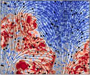



1. Introduction
Turbulent entrainment of ambient fluid into the primary flow, which holds significant importance in a diverse range of geophysical and industrial flows, has captivated the attention of both physicists and engineers for an extended period (e.g. Turner Reference Turner1986; Hallworth et al. Reference Hallworth, Phillips, Huppert and Sparks1993; Hunt & Burridge Reference Hunt and Burridge2015; Mellado Reference Mellado2017). The instantaneous boundary between the primary turbulent flow and the background is characterized by a thin layer demarcating the turbulent primary flow from the ambient, which is usually referred to as the turbulent/non-turbulent interface (TNTI) when the background flow is non-turbulent and irrotational (Corrsin & Kistler Reference Corrsin and Kistler1955; Townsend Reference Townsend1976; da Silva et al. Reference da Silva, Hunt, Eames and Westerweel2014). More generally, the background flow can also be turbulent, such as in the confluence of different rivers (Sukhodolov et al. Reference Sukhodolov, Shumilova, Constantinescu, Lewis and Rhoads2023) or in the wakes of wind turbines developing in the atmospheric boundary layer and the wake of upstream machines (Porté-Agel, Bastankhah & Shamsoddin Reference Porté-Agel, Bastankhah and Shamsoddin2020). In such cases, the interface is referred to as the turbulent/turbulent interface (TTI) (e.g. Kankanwadi & Buxton (Reference Kankanwadi and Buxton2020) and Kohan & Gaskin (Reference Kohan and Gaskin2022)). The dynamics of the bounding interface, whether TNTI or TTI, has a direct influence on the turbulent entrainment processes and hence dictates the flux of transportable quantities, such as mass, momentum, energy and other scalars (Townsend Reference Townsend1976; Buxton & Chen Reference Buxton and Chen2023; Huang, Burridge & van Reeuwijk Reference Huang, Burridge and van Reeuwijk2023).
In the past decades, studies of TNTIs have advanced our understanding of entrainment and mixing into turbulent flows remarkably. The convoluted surface has proven to be self-similar and fractal, which revealed the intricate multiscale nature of the entrainment processes (Sreenivasan, Ramshankar & Meneveau Reference Sreenivasan, Ramshankar and Meneveau1989; Mistry et al. Reference Mistry, Philip, Dawson and Marusic2016; Chen et al. Reference Chen, Tang, Fan and Jiang2024). Entrainment occurring at small scales, referred to as ‘nibbling’, results from the outward viscous diffusion of the fluctuating vorticity of the turbulent flow; on the contrary, large-scale entrainment, so-called ‘engulfment’, is a consequence of the inviscid action of the large-scale vortical structures. The dominant mechanism of entrainment, either the viscous ‘nibbling’ or the inviscid ‘engulfment’, is still a subject of debate. While ‘nibbling’ seems to be the principal mechanism of entrainment (e.g. Corrsin & Kistler Reference Corrsin and Kistler1955; Mathew & Basu Reference Mathew and Basu2002; Westerweel et al. Reference Westerweel, Fukushima, Pedersen and Hunt2005, Reference Westerweel, Fukushima, Pedersen and Hunt2009; Watanabe et al. Reference Watanabe, Sakai, Nagata, Ito and Hayase2015; Stella, Mazellier & Kourta Reference Stella, Mazellier and Kourta2017), ‘engulfment’ is more likely to be prominent when large-scale coherent motions prevail in the flow (e.g. Brown & Roshko Reference Brown and Roshko1974; Yule Reference Yule1978; Dahm & Dimotakis Reference Dahm and Dimotakis1990; Bisset, Hunt & Rogers Reference Bisset, Hunt and Rogers2002; Chauhan et al. Reference Chauhan, Philip, De Silva, Hutchins and Marusic2014; Cimarelli & Boga Reference Cimarelli and Boga2021). It is also noted that Mistry et al. (Reference Mistry, Philip, Dawson and Marusic2016) demonstrated that the entrainment mass flux is scale-independent based on their observation that the mean entrainment velocity scales such that it balances the scaling of the interface surface area, which leads to their product remaining constant when perceived at different length scales.
In contrast to the extensive studies on TNTIs in the past decades, the investigation of TTIs has only started to intensify in recent years, despite their widespread existence in many applications. The persistence of TTIs between two distinctive turbulent flows has now been verified by both experimental and numerical studies (Kankanwadi & Buxton Reference Kankanwadi and Buxton2020, Reference Kankanwadi and Buxton2022; Kohan & Gaskin Reference Kohan and Gaskin2022; Huang et al. Reference Huang, Burridge and van Reeuwijk2023; Nakamura, Watanabe & Nagata Reference Nakamura, Watanabe and Nagata2023), even in cases where the turbulence intensities of the primary flow and the background are comparable to one another, something that had been previously doubted (da Silva et al. Reference da Silva, Hunt, Eames and Westerweel2014). The presence of turbulence in the background flow has a profound effect on the entrainment across the interface. Kankanwadi & Buxton (Reference Kankanwadi and Buxton2020) demonstrated that higher turbulence intensity in the background effectively suppresses the mass entrainment rate (with respect to a non-turbulent background) in the far-field of a planar wake, which was attributed to the increased prevalence of detrainment events caused by the free-stream turbulence (FST) (Kohan & Gaskin Reference Kohan and Gaskin2024). Interestingly, in their later study of the entrainment in a cylinder's near wake (within 11 diameters of the cylinder downstream), Kankanwadi & Buxton (Reference Kankanwadi and Buxton2023) found that turbulence intensity and integral length scale cooperate to enhance the entrainment of background fluid into the wake (with respect to a non-turbulent background), as long as the coherent von Kármán vortices are not eliminated from the wake. These contrasting observations in the near- and far-fields of the wake highlight the vigorous evolution of the inherent features of the TTI as the wake's coherent vortices diminish downstream. One may expect there must be a ‘crossover location’ of the characteristics of the interface between the two states in the near- and far-fields, which was indeed observed by Chen & Buxton (Reference Chen and Buxton2023) in the intermediate wake at approximately 15 diameters downstream from the cylinder (at the particular Reynolds number studied). They showed that the wake bounding interface spreading rate is evidently reduced and the mean interface position starts to scale with the local wake half-width downstream of this position, as observed in the axisymmetric self-similar wake in Zhou & Vassilicos (Reference Zhou and Vassilicos2017).
Several intriguing questions arise from the observation of Chen & Buxton (Reference Chen and Buxton2023) of the transition of the characteristics of TTIs during the wake's evolution downstream. What are the underlying physics responsible for this change of wake spreading? Is it a manifestation of the large-scale coherent vortices of the wake modifying various features of the interface, and the extent to which this evolves as the coherent vortices diminish in significance? More importantly, how does the vorticity field near the interfacial layer change before and after the transition position, particularly its scaling? How does such a change of the vorticity dynamics affect the entrainment velocity? All these questions motivated the current work in which simultaneous, combined particle image velocimetry (PIV) and planar laser-induced fluorescence (PLIF) measurements were carried out to observe the details of the evolution of the velocity and vorticity fields in the vicinity of the interfacial layer.
The paper is organized as follows. Section 2 introduces the details of the PIV and PLIF experiments and the methodology employed to determine the interface position within the flow. The major results are discussed in § 3 and we conclude the work in § 4.
2. Experimental set-up and interface detection
2.1. Experimental set-up
The experiments were similar to those in Buxton & Chen (Reference Buxton and Chen2023) and were conducted in the water flume of the hydrodynamics laboratory of the Department of Aeronautics at Imperial College London. A cylinder with a diameter  $d = 1$ cm was vertically mounted in the middle of the test section (figure 1a). The incoming velocity of the flow was
 $U_\infty = 0.38$ m s
 $^{-1}$, and the Reynolds number based on
 $U_\infty$ and
 $d$ was approximately 3800. There was a turbulence-generating grid installed upstream of the cylinder to generate the background turbulence. Four different grids (including two regular grids and two fractal grids, see Kankanwadi & Buxton (Reference Kankanwadi and Buxton2020) for details) were utilized and the distance between the grid and the cylinder was adjusted such that the integral length scale
 $\mathcal {L}\ (\equiv \int ^{r_0}_0 R_{12}(r) \,\mathrm {d}r$ where
 $R_{12}(r)$ is the correlation function between velocity fluctuations
 $u^\prime (x, y)$ and
 $u^\prime (x, y+r)$, and
 $r_0$ is the first zero-crossing of
 $R_{12}$) and the turbulence intensity
 $k\ (\equiv\sqrt{(\overline{u^{\prime 2}}+\overline{v^{\prime 2}})/2}/U_\infty$, where the overbar denotes averaging over time) of the background turbulence was varied independently (figure 1c). The cases are divided into three groups based on the background turbulence intensity in which case 1a is that with no grid placed upstream of the cylinder, which serves as the closest representation of a TNTI under our experimental constraints. The variation of
 $k$ and
 $\mathcal {L}$ with respect to their values at
 $x/d = 20$, within the streamwise extent of the measurements, is approximately
 $2\,\%$ and 0.1
 $d$, respectively, for the cases using regular grids (cases 2a, 3a, 3b in figure 1c); for the cases using fractal grids (cases 1b, 1c and 2b) the variations are approximately
 $1\,\%$ for
 $k$ and
 $0.5d$ for
 $\mathcal {L}$. These variations do not affect the relative positions to one another of the FST cases in figure 1(c). The coordinate system is a standard
 $(x,y)$ Cartesian system where the origin is the centre of the cylinder and
 $x$ is the streamwise coordinate (figure 1b).
(a) Conceptual sketch of the experimental set-up. (b) Configuration of the measurement FoV. (c) Parameter space ( $k$,
 $\mathcal {L}$) of the background flow in the
 $x/d = 20$ measurement station.

Simultaneous measurements via PLIF and PIV were carried out with measurements centred at five streamwise positions, i.e.  $x = 6.5d$, 10
 $d$, 20
 $d$, 30
 $d$ and 40
 $d$. In the PIV system, two cameras (Phantom V641 with sensor resolution of
 $2560\times 1600$ pixels) were arranged in the cross-stream (
 $\kern0.09em y$) direction, each of which has a field of view (FoV) of
 $5d \times 3d$. They together formed a combined FoV of
 $9d \times 3d$ with a
 $1d$ overlap in the
 $y$ direction (figure 1b). The combined FoV was thus large enough to capture all the possible interface positions at all the examined streamwise locations. The PLIF camera was located on the opposite side of the flume to the PIV cameras (figure 1a) with a FoV large enough to encompass that of the combined PIV FoV (shown later in figure 3b).
Table 1 provides a summary of the relevant parameters of the PIV and PLIF experiments. Hollow glass spheres with a mean diameter of  $10\ \mathrm {\mu }$m were used to seed the flow for the PIV measurements. The appropriateness of choosing such seeding particles was discussed in Kankanwadi & Buxton (Reference Kankanwadi and Buxton2020). A high-speed Nd:YLF laser (Litron LDY304) with wavelength of 527 nm was used to illuminate the flow. A fluorescent dye, Rhodamine 6G, was employed to demarcate the wake region of the cylinder from the background flow. When exposed to the laser illumination the dye emits light of wavelength approximately 560 nm, so a low-pass filter was used for the PLIF camera to avoid contamination of the images with light scattered from the tracer particles, and a bandpass filter centred on 532 nm was used for the PIV cameras to reject the fluorescent light. The dye has a high Schmidt number (
 $Sc$, approximately 2500 in water) which ensures that the molecular diffusion of the dye is negligibly small compared with the turbulent motions. Accordingly, the dye can be treated as a passive scalar and displays clear boundaries of concentration; the small Batchelor scale
 $\eta _B (\equiv \eta /Sc^{1/2}$ where
 $\eta$ is the Kolmogorov length scale) makes the details of the dye interface negligibly small in comparison with those of the vorticity interface. The dye was released into the wake from a hole in the rear surface of the cylinder with the aid of a microdosing pump (Bürkert 7615) working at a constant frequency of 20 Hz. This method has been previously shown to faithfully mark the extent of the wake from almost immediately downstream of the cylinder (Kankanwadi & Buxton Reference Kankanwadi and Buxton2020). A 2-m-long elastic tube connecting the pump to the release-hole was used to smooth the stroking of the pump. The acquisition frequency
 $f_{ac}$ of both PIV and PLIF cameras was 200 Hz and 5000 velocity fields/concurrent PLIF images were captured for each measurement.
Some parameters of the PIV and PLIF experiments.

The PIV processing was conducted via the programme PIVlab, an open-source toolbox of MATLAB, which features multipass and multigrid with image deformation (Thielicke & Sonntag Reference Thielicke and Sonntag2021). Four passes were carried out during the analysis and the final IW size was  $24 \times 24$ pixels with 50 % overlap, which corresponds to a
 $0.48\ {\rm mm} \times 0.48\ {\rm mm}$ interrogation window in physical space. Achieving a high spatial and temporal resolution is vital to studying entrainment, whether experimentally or numerically, since entrainment processes typically occur at length and time scales that are similar to the Kolmogorov length and time scales. Figure 2 shows the spatial and temporal resolution of the current measurements in terms of the ratio of IW size
 $L_{IW}$ to the Kolmogorov length scale on the interface
 $\eta _I$ (
 $\equiv (\nu ^3/\varepsilon _I)^{1/4}$ where
 $\nu$ is kinematic viscosity of water and
 $\varepsilon _I$ is the turbulent kinetic energy dissipation rate ensemble-averaged on the interface) and the ratio of the period of acquisition
 $T_{ac}\ (= 1/f_{ac})$ to the Kolmogorov time scale on the interface
 $\tau _{\eta, I}\ (\equiv (\nu /\varepsilon _I)^{1/2})$, respectively, for all the cases from
 $x/d = 6.5$ to
 $x/d = 40$. For all cases, both the spatial and temporal resolution of the measurements improves with distance downstream due to the reduced turbulent kinetic energy dissipation rate which is estimated from the PIV measurements by using a locally axisymmetric assumption, e.g.
 $\varepsilon _I = \nu (-\langle u_{,x}^2 \rangle _I + 2\langle u_{,y}^2\rangle _I+2\langle v_{,x}^2\rangle _I+8\langle v_{,y}^2\rangle _I)$ where
 $u,_{\alpha } \equiv \partial u/\partial \alpha$ (see George & Hussein Reference George and Hussein1991; Chen et al. Reference Chen, Cuvier, Foucaut, Ostovan and Vassilicos2021) and
 $\langle {\cdot } \rangle _I$ denotes the conditionally averaged value on the interface (see § 2.3). The spatial resolution
 $L_{IW}/\eta _I$ ranges from approximately 4–5 in the very near wake to approximately 2–4 in the farthest downstream position, and the temporal resolution is always below 0.6 for all the cases at all measured positions. The relatively high temporal and spatial resolution for these experiments justifies the use of planar PIV, since achieving sufficiently high spatial and temporal resolution becomes challenging with three-dimensional techniques such as tomographic PIV.
Spatial and temporal resolution of the measurements. (a) The ratio of IW size  $L_{IW}$ to the Kolmogorov length scale on the interface
 $\eta _I$. (b) The ratio of the period of acquisition
 $T_{ac}$ to the Kolmogorov time scale on the interface
 $\tau _{\eta, I}$.

2.2. Interface detection
Following previous studies of TTIs (e.g. Kankanwadi & Buxton Reference Kankanwadi and Buxton2020; Kohan & Gaskin Reference Kohan and Gaskin2022, Reference Kohan and Gaskin2024), the interface is identified from the boundary of the fluorescent dye captured by the PLIF camera. Note that turbulent fluid appears on both sides of the interface and hence vorticity magnitude is not a suitable metric for identifying a TTI. In the detection process, the PLIF images were first normalized by the mean light intensity on the wake centreline ( $\kern0.09em y = 0$), i.e.
 $\phi ^* (t, x, y) = \phi (t, x, y)/\bar {\phi }(x, y = 0)$. This makes the light intensity of all the images approximately similar for all downstream distances, which benefits the use of the same threshold value for the whole ensemble of images. For each PLIF image, the magnitude of the gradient of the normalized light intensity is calculated as
 $\varGamma ^* \equiv |\boldsymbol {\nabla } \phi ^*|$. A conditional average was taken of
 $\varGamma ^*$ exceeding the given threshold value
 $\varGamma ^*_{th}$, i.e.
 \begin{equation} \widehat{\varGamma^*} = \frac{\sum (\varGamma^*\,|\,\varGamma^* > \varGamma^*_{th} )}{N(\varGamma^* > \varGamma^*_{th})}. \end{equation}
The distribution of  $\widehat {\varGamma ^*}$ with respect to
 $\varGamma ^*_{th}$ for the non-turbulent background (case 1a in figure 1c) is shown in figure 3(a). Here
 $\widehat {\varGamma ^*}$ increases slowly first for small
 $\varGamma ^*_{th}$. As
 $\varGamma ^*_{th}$ increases, as expected,
 $\widehat {\varGamma ^*}$ surges rapidly after a knee point which is evidently depicted by the gradient
 $\mathrm d \widehat {\varGamma ^*}/ \mathrm d \varGamma ^*_{th}$. The value of
 $\varGamma ^*_{th}$ corresponding to the knee point demarcates the limit of the level of
 $\varGamma ^*$ in the background from that in the wake (see Prasad & Sreenivasan Reference Prasad and Sreenivasan1989; Chen & Buxton Reference Chen and Buxton2023). With the threshold value
 $\varGamma ^*_{th}$ determined nearby to the knee point (marked with a dashed line in figure 3a), the interface can be effectively identified in the PLIF image (black line in figure 3b). The envelope of the determined interface, which is obtained from the line connecting the outermost points of the interface at each
 $x$ location (the red line in figure 3b), is then projected onto the PIV velocity field measured at the same time instant, as shown in figure 3(c). The good agreement between the determined interface and the boundary of the vorticity field in figure 3(c) illustrates the effectiveness of the methodology adopted.
(a) Distribution of  $\widehat {\varGamma ^*}$ and
 ${\rm d} \widehat {\varGamma ^*} / {\rm d} \varGamma ^*_{th}$ with respect to
 $\varGamma ^*_{th}$. (b) The determined interface (black line) in a typical PLIF image using the threshold in (a) and the resultant interface-envelope (red line) in the PIV FoV. (c) Enstrophy field measured by the PIV at the same moment as (b) with the envelope (black line) determined in (b).

It is noted that the decay of the concentration of the fluorescent dye as the flow spreads downstream can cause the fluorescent light intensity to be attenuated, which may lead to errors in the interface detection at these downstream positions. In order to test whether the dye concentration is sufficient for the detection of the interface at  $x/d =40$, we performed a conditional average of the light intensity gradient
 $\varGamma ^*$ with respect to the interface position, which is determined with the method depicted in figure 3, for all the FST cases at
 $x/d = 40$. The details of the conditional averaging technique are given in § 2.3. As shown in figure 4, for all cases, the distribution of the conditionally averaged light intensity gradient
 $\langle \varGamma ^* \rangle$ with respect to the interface-normal coordinate
 $\xi _n$ (see figure 6 for the definition of
 $\xi _n$), displays a very sharp jump across the determined interface position,
 $\xi _n = 0$. The clear jumps of
 $\langle \varGamma ^* \rangle$ indicate that the concentration of the fluorescent dye inside the wake is high enough to identify the interface for all cases at
 $x/d = 40$. Note also that due to the (ubiquitous) presence of experimental noise
 $\varGamma ^\ast$ can be locally/instantaneously larger than the time-averaged value that identifies the start of the rise of
 $\langle \varGamma ^* \rangle (\xi _n)$. Accordingly, interface-identification using the threshold defining the red dashed line yields noisy and/or unphysical interface lines and a slightly larger value of
 $\varGamma ^\ast _{th}$, selected according to the methodology of figure 3(a), is necessary for accurate interface identification. The chosen threshold value
 $\varGamma ^\ast _{th}$ is denoted in figure 4 with the horizontal dashed black line. Consequently, the determined interface (
 $\xi _n = 0$ marked as a vertical black dashed line in figure 4) may be slightly offset from the very position where
 $\langle \varGamma ^* \rangle (\xi _n)$ starts to rise (marked with a red dashed line in figure 4). If we take the red-dashed line as a reference then the offset/error to the identified interface for all cases at
 $x/d= 40$ can be estimated as the difference between the two positions which is approximately
 $0.02d$ (i.e. approximately 1.3
 $\eta _I$). Nevertheless, as figure 3(c) shows the chosen threshold value satisfactorily identifies all TTIs and the TNTI and
 $1.3 \eta _I$ is an upper limit on our uncertainty of the interface position.
Distributions of conditionally averaged PLIF light intensity gradient  $\langle \varGamma ^* \rangle$ for all cases at
 $x/d = 40$. The vertical black dashed line denotes the position of the detected interface (
 $\xi _n = 0$), the red dashed line denotes the reference position of the interface at which
 $\langle \varGamma ^\ast \rangle (\xi _n)$ begins to rise, and the horizontal dashed line denotes the level of the threshold used to detect the interface. For all the FST cases at
 $x/d = 40$,
 $\varGamma ^*_{th} = 0.008$.

To ensure both TNTIs and TTIs at different  $x/d$ locations can be identified reliably, the method is tested on all seven cases at the five examined
 $x/d$ positions. Figure 5 shows typical examples of the interface identification of one TTI case, with intermediate background
 $k$ (case 2b), and the TNTI case (case 1a) for all
 $x/d$ locations. It should be noted that although the profiles of
 $\widehat {\varGamma ^*}$ for the TNTI and all TTI cases at all
 $x/d$ positions are similar, the threshold value
 $\varGamma ^*_{th}$ is both case- and position-dependent. From
 $x/d = 6.5$ to
 $x/d = 40$, both the interfaces of the turbulent/turbulent case and the turbulent/non-turbulent case are effectively captured and agree well with those identified from the vorticity field. It is interesting to see that the geometric features of TTIs are perceptibly different to those of the TNTI, which has been examined in detail in Chen & Buxton (Reference Chen and Buxton2023) based on a PLIF only experiment. In the following sections, the effect of the background turbulence on the nature of the interfaces, and the entrainment across them, is to be studied mainly based on the PIV data (the PLIF data is simply used to identify the interface position).
Examples of (a–e) a TTI (case 2b) and (f–j) a TNTI (case 1a) at (a,f)  $x/d = 6.5$; (b,g) 10; (c,h) 20; (d,i) 30; (e,j) 40.

2.3. Conditional-averaging methodology
In this work, a conditional-averaging method, with respect to the position of the determined interface envelope, is adopted to examine the flow field in the vicinity of the interface. This methodology is similar to that used in previous studies (e.g. Westerweel et al. Reference Westerweel, Fukushima, Pedersen and Hunt2005, Reference Westerweel, Fukushima, Pedersen and Hunt2009; Yu & Lu Reference Yu and Lu2019; Kankanwadi & Buxton Reference Kankanwadi and Buxton2020). Figure 6 illustrates the application of the technique. The averaging is conducted spatially over the streamwise extent of the identified interfaces in each PIV FoV, as well as temporally, i.e. over all PIV velocity fields, on the condition of distance-to-the-interface along the interface-normal direction (thick black lines in figure 6). The statistics are generated over the range  $-0.4d \leq \xi _n \leq 0.4d$ with the origin set to the detected interface location. The direction pointing into the wake region is defined as being positive (
 $\xi _n > 0$ in figure 6). It should be noted that those samples whose path from
 $-0.4d$ to 0.4
 $d$ passes through the interface more than once (like the dashed lines in figure 6) are excluded from the averaging sample to avoid contaminating the result. The typical resultant ensemble size is approximately
 $1\unicode{x2013}2\times 10^5$ which has been checked to be enough to converge the statistics.
 $\xi _t$ is the tangential direction of the local interface coordinate system
 $(\xi _t, \xi _n)$ with
 $\xi _t > 0$ pointing downstream. The resultant average is denoted as
 $\langle {\cdot } \rangle$, and
 $\langle {\cdot } \rangle _I$ is the averaged value on the interface, i.e.
 $\langle {\cdot } \rangle (\xi _n = 0)$.
Illustration of the conditional averaging method with respect to the interface location (black line). The contours depict  $\omega _z^2$. Solid black lines normal to the local interface are exemplar positions considered to be valid, i.e. the interface is only crossed once. Dashed black lines are considered invalid (multiple interface-crossings) and are hence rejected from the conditional-averaging ensemble. (
 $\xi _t, \xi _n$) is the local interface coordinate system for the conditional averaging.

3. Results and discussion
3.1. Conditionally averaged velocity and vorticity profiles across the TTIs
As the wake develops downstream, from  $x/d = 6.5$ to
 $x/d = 40$, the flow is subjected to a strong evolution such that the dominant von Kármán vortices (in the near wake) experience a substantial energetic decay and variation in topology (e.g. Chen et al. Reference Chen, Zhou, Antonia and Zhou2018; Jiang et al. Reference Jiang, Hu, Cheng and Zhou2022). Consistent with such variation of these structures, the probability density functions (PDFs) of both TNTI- and TTI-position (relative to the wake centreline) were observed to evolve from being distinctly non-Gaussian in the near wake to being Gaussian in the far-field (Chen & Buxton Reference Chen and Buxton2023). In this section, the primary focus is thus on how the velocity and vorticity fields in proximity to the TTIs undergo changes as the flow develops downstream.
We first focus on the conditionally averaged velocity profile across the various interfaces. Figure 7 shows the distributions of the conditionally averaged (§ 2.3) streamwise and lateral velocities  $\langle U \rangle$ and
 $\langle V \rangle$ for all seven cases denoted in figure 1(c) at various measurement stations from
 $x/d = 6.5$ to 40. Here
 $\langle U \rangle$ is normalized by the mean velocity at the interface
 $\langle U \rangle _I$ so as to highlight the mean shear
 $\mathrm d\langle U \rangle /\mathrm d\xi _n$ of the interfacial layer for different cases which is important in affecting the vorticity jump across the interface and the entrainment velocity (Wolf et al. Reference Wolf, Holzner, Lüthi, Krug, Kinzelbach and Tsinober2013). Although the mean shear for all cases decays noticeably as the flow evolves downstream, FST has a substantial effect on the mean shear strength, especially in the far-field of the wake. At
 $x/d = 6.5$ (figure 7a),
 $\langle U \rangle /\langle U \rangle _I$ for all cases drops at a similar rate nearby to the interface (
 $\xi _n \approx 0$) on the wake side. It indicates that the mean shear across the interfacial layer in the near wake is robustly dominated by the motion of the wake itself, such as the strong rotational motion of the von Kármán vortices which can give rise to a high strain rate near to the wake boundary. Farther downstream (figure 7b–d), the importance of the FST seems to increase. Note that the cases with higher FST intensities (group 3 in figure 1c) generally degrade faster than those with lower ones (groups 1 or 2 in figure 1c). Especially at
 $x/d = 40$ (figure 7d), the mean shears of cases 3a and 3b are almost imperceptible, while the cases of group 1 still maintain a noticeable mean shear with cases in group 2 lying somewhere in between. As the mean shear across the interfacial layer plays a role in enhancing the local entrainment velocity (Wolf et al. Reference Wolf, Holzner, Lüthi, Krug, Kinzelbach and Tsinober2013), one may expect that the entrainment velocity across TTIs in the far-field is thus reduced in comparison with a TNTI, which is indeed observed in the current study (shown later in figure 14a). This could also partly explain the suppression of mass entrainment in the far wake of TTIs observed in Kankanwadi & Buxton (Reference Kankanwadi and Buxton2020).
Streamwise evolution of the conditionally averaged velocity (a–d)  $\langle U\rangle /\langle U\rangle _I$ and (e–h)
 $\langle V\rangle /U_\infty$ across the TNTI and TTIs for all cases at (a,e)
 $x/d = 6.5$; (b,f) 10; (c,g) 20; (d,h) 40.

Compared with the rapid change of the streamwise velocity across the interfacial layer, the transverse velocity  $\langle V \rangle /U_\infty$ crosses the layer more continuously (figure 7e–h). For all cases,
 $\langle V \rangle /U_\infty$ generally displays negative values on the free-stream side of the interface (
 $\xi _n < 0$) and positive values on the wake side (
 $\xi _n > 0$), which indicates that the local velocity field tends to compress the TNTI/TTI. A similar observation was also made in the TNTI of mixing layers (Jahanbakhshi & Madnia Reference Jahanbakhshi and Madnia2018) and turbulent boundary layers (Chauhan et al. Reference Chauhan, Philip, De Silva, Hutchins and Marusic2014). The positive
 $\langle V \rangle /U_\infty$ on the wake side is a reflection of the transverse spreading of the wake towards the ambient free stream, and the negative
 $\langle V \rangle /U_\infty$ outside the interface manifests the ambient fluid moving towards the wake due to the entrainment of the wake (Bisset et al. Reference Bisset, Hunt and Rogers2002). Note that at
 $x/d = 6.5$ (figure 7e)
 $\langle V \rangle /U_\infty$ changes sign, for all cases, slightly towards the wake side of the interface (
 $\xi _n \gtrsim 0$). We confirmed that the zero-position of
 $\langle V \rangle (\xi _n)$ for each case coincides with the location of the maximum mean shear
 $\mathrm {d}\langle U \rangle /\mathrm {d}\xi _n$, particularly evident when the background turbulence is not intense. As
 $x/d$ increases to 40 (figure 7h), in accordance with the reduced mean shear (figure 7d), the zero-position of
 $\langle V \rangle /U_\infty$ evolves gradually towards the defined-interface position (
 $\xi _n = 0$).
The strong streamwise evolution of the conditionally averaged velocity field in proximity to the interface suggests that there is also an intense streamwise variation in the conditionally averaged vorticity field, which will have a direct influence on the small-scale entrainment processes across the interface (e.g. Holzner & Lüthi Reference Holzner and Lüthi2011; Wolf et al. Reference Wolf, Lüthi, Holzner, Krug, Kinzelbach and Tsinober2012). Since only the spanwise component  $\omega _z$ of the vorticity vector
 $\boldsymbol {\omega }$ is available from the planar PIV measurements, we adopt the squared spanwise vorticity
 $\omega _z^2$ as a surrogate for the enstrophy
 $\omega ^2$(
 $\equiv \boldsymbol {\omega }\boldsymbol {\cdot } \boldsymbol {\omega }$). Taveira & da Silva (Reference Taveira and da Silva2013) reported that the magnitudes of the three vorticity components across the interface are approximately equal. Subsequently, later in figure 9 we indirectly infer that
 $\langle \omega_z^2 \rangle \approx \langle \omega^2 \rangle /3$ in the region of quasihomogeneous turbulence on either side of the interface. Accordingly, the scaling of
 $\langle \omega_z^2 \rangle$ should preserve the essential scaling features of the enstrophy field
 $\langle \omega^2 \rangle$ which are of interest to us.
The conditionally averaged vorticity  $\langle \omega _z^2 \rangle$ for the various cases of TTIs and the TNTI, from
 $x/d = 6.5$ to
 $x/d = 40$, is shown in figure 8. As expected, for all cases, there is a clear jump of the vorticity initiating at the outermost surface of the interface (
 $\xi _n = 0$), although the magnitude of the jump decays as the flow progresses downstream. For all measurement locations, the vorticity jump across the TTIs is generally larger than that across the TNTI, similar to the observation made in Kankanwadi & Buxton (Reference Kankanwadi and Buxton2020). It is interesting to see that at the farthest downstream location
 $x/d = 40$ (figure 8d), for some TTI cases (e.g. cases 3a and 3b), even though the background vorticity level is comparable to that inside the wake and the mean shear of the interfacial layer is negligibly small (case 3a and 3b in figure 7d), the vorticity jump still exists. This feature suggests that the existence of TTIs is mainly a result of the difference between the local vorticity fields on either side of the interface, which we shall see later in figure 19.
Conditionally averaged enstrophy  $\omega _z^2/(U_\infty /d)^2$ at
 $x/d = (a)$ 6.5; (b) 10; (c) 20; (d) 40 for all cases. The shaded area represents the 95 % confidence interval.

In light of the evident decay of the magnitude of the vorticity jump across the TTIs as they evolve downstream, a particularly interesting question is whether the scaling of the vorticity varies in this process? We first examine the scaling of the vorticity from  $x/d = 20$ to 40 in figure 9. In this figure, the jump of
 $\langle \omega _z^2 \rangle$ for the cases with low (figure 9a,c,e) and high (figure 9b,d,f) background turbulence intensities are presented separately. Consistent with figure 8, the vorticity jump for all cases decreases monotonically downstream when they are normalized by the invariant quantities of incoming velocity
 $U_\infty$ and cylinder diameter
 $d$ (figure 9a,b). As vorticity predominantly resides in the small scales, it is natural to expect the vorticity field close to the interface to scale with the Kolmogorov scales, both length and time (e.g. Hunt et al. Reference Hunt, Eames, Da Silva and Westerweel2011). Here we compare two possible choices of the Kolmogorov length scale, based on different dissipation rates which are estimated in the same way as introduced in § 2.1. One possible choice is a dissipation rate representative of the turbulent core of the wake, but still in proximity to the interface. For this we select the dissipation rate
 $\varepsilon _p$ at the
 $\xi _n$-position where the profile of
 $\langle \omega _z^2 \rangle$ plateaus on the wake side of the interfaces, as indicated by the dashed line in figure 9(a,b). With such a normalization, based on
 $\varepsilon _p$, the distributions of
 $\langle \omega _z^2 \rangle$ for the various cases with various background turbulence intensities from
 $x/d = 20$ to
 $x/d = 40$ follow each other fairly well on the wake side of the interfaces (
 $\xi _n/\eta _p>0$ in figure 9c,d, where
 $\eta _p$ is the Kolmogorov length scale based on
 $\varepsilon _p$). The plateau value of
 $\langle \omega _z^2 \rangle /(\varepsilon _p/\nu )$ is approximately 1/3 in the wake region for all cases, which is reasonable given that we have one vorticity component of the full enstrophy measured and the magnitude of the three components of enstrophy in the turbulent core region ought to be comparable to one another in a fully developed (homogeneous, isotropic) turbulent flow (e.g. Taveira & da Silva Reference Taveira and da Silva2013). Note that for fully homogeneous turbulence, the mean dissipation rate is equivalent to the product of viscosity and mean enstrophy, i.e.
 $\langle \omega^2 \rangle/(\varepsilon /\nu ) = 1$ (Tennekes & Lumley Reference Tennekes and Lumley1972; Zecchetto & da Silva Reference Zecchetto and da Silva2021).
Scaling of  $\langle \omega _z^2\rangle$ in (a,c,e) low and (b,d,f) high background turbulence intensities. Panels (a,b) show
 $\langle \omega _z^2 \rangle$ and
 $\xi _n$ normalized with invariant length/time scales
 $d$ and
 $U_\infty$. Panels (c,d) show
 $\langle \omega _z^2 \rangle$ normalized by the plateau value of the dissipation rate at
 $\xi_n$ indicated by the dashed line in (a,b) and
 $\xi _n$ normalized by the Kolmogorov length scale formed from the plateau dissipation rate. Panels (e,f) are normalized with the local dissipation rate
 $\varepsilon _l(\xi _n)$.

However, it is clear that in the background-side of the TTI, outside of the wake ( $\xi _n/\eta _p<0$), the vorticity field does not scale with the Kolmogorov scale from the turbulent core of the wake, especially when the background turbulence intensity is high (figure 9d). This is not unexpected since the vorticity field in the neighbourhood of the interface features high inhomogeneity (figure 9d), so the Kolmogorov scaling can only be expected to apply locally. Zecchetto & da Silva (Reference Zecchetto and da Silva2021) reported that the statistics of the enstrophy across TNTIs universally scale with the local Kolmogorov velocity and length scales for different free-shear flows. Following their method, we normalize
 $\langle \omega _z^2 \rangle$ of the examined cases using the local dissipation rate (
 $\varepsilon _l$) as a function of
 $\xi _n$-position in figure 9(e,f). It is interesting to see that the shapes of
 $\langle \omega _z^2 \rangle$ for the various cases are quite different from those normalized by the dissipation rate from the wake core in figure 9(c,d), especially in the background region outside of the wake (
 $\xi _n<0$). When the background turbulence intensity is low (figure 9e), the distributions of
 $\langle \omega _z^2 \rangle$ for different cases diverge widely; on the contrary, for the cases with high background turbulence intensity (figure 9f), the distributions of
 $\langle \omega _z^2 \rangle$ outside the wake (
 $\xi _n<0$) collapse, similarly to those within the wake (
 $\xi _n>0$). Although one might expect that the enstrophy
 $\langle \omega _z^2 \rangle$ scaling with local Kolmogorov scales
 $\varepsilon _l/\nu$ (
 $=(u_\eta /\eta )^2$ where
 $u_\eta$ and
 $\eta$ are, respectively, the Kolmogorov velocity and length scales) is consistent with homogeneous turbulence, which is approximately attained far away from the interface on either side of the TTIs in figure 9(f), it is the collapse of the curves in the inhomogeneous neighbourhood of the interface that is of particular interest. A similar symmetric enstrophy profile of
 $\langle \omega ^2 \rangle$ was also observed in a recent direct numerical simulation of a TTI in grid-generated shear-free turbulence (Nakamura et al. Reference Nakamura, Watanabe and Nagata2023).
These observations merit some additional comments. First, it is clear that the profiles of  $\langle \omega _z^2 \rangle$ scale better with the local dissipation rate/Kolmogorov scale (figure 9e,f) than they do with the values in the wake core (figure 9c,d). This observation seemingly broadens the applicability of the universality of the scaling of the conditional mean enstrophy jump across the interface with the local small-scale phenomenology from TNTIs, first reported by Zecchetto & da Silva (Reference Zecchetto and da Silva2021), to TTIs. Second, the structure of TTIs seems to be different from that of the TNTI in that there are two distinct layers established in the former (figure 9f) with one on each side of the defined-interface (
 $\xi _n = 0$) whereas contrastingly there is only one distinct layer formed in the latter (case 1a in figure 9e). Note when referring to ‘distinct’ layers we are doing so based on the normalized conditional mean enstrophy jump (i.e. a jump in enstrophy from
 $\xi _n = 0$ to a peak on either side) and not, for example, considering the transition from the viscous superlayer to the turbulent sublayer, the two constituent sublayers of a TNTI (da Silva et al. Reference da Silva, Hunt, Eames and Westerweel2014), whose distinction is typically only apparent when considering the various terms of the enstrophy transport equation.
The two layers of the TTIs seemingly result from different physical mechanisms. The layer on the wake side ( $\xi _n >0$) is apparently a manifestation of the rapid vorticity jump from the ambient flow to the wake (figure 9a,b). As such a vorticity jump does not appear in the layer on the free-stream side of the TTI (
 $\xi _n < 0$ in figure 9a,b), then the normalization with
 $\varepsilon _l$ must be responsible. One can expect that the distribution of
 $\varepsilon _l$ in the vicinity of the interface on the free-stream side must be very different between the cases with high and low FST intensities. This conjecture is supported by the contrasting distributions of the dissipation rate
 $\varepsilon _l$ in the interfacial region between the wake and the ambient flow with different levels of background turbulence intensities presented in figure 10, particularly in the region of the second layer (
 $-13\eta _l < \xi _n < 0$). When the ambient turbulence intensity is low (figure 10a, which corresponds to the FST cases in figure 9e),
 $\varepsilon _l$ drops rapidly from the wake to the ambient flow in the region of the first layer (
 $0 < \xi _n < 13\eta _l$) and is approximately homogeneous in the region of the second layer (
 $-13\eta _l < \xi _n < 0$), with a similar level to the ambient flow. Contrastingly, when the ambient turbulence intensity is high (figure 10b, corresponding to the same FST cases as in figure 9f), the transition of
 $\varepsilon _l$ from the wake to the ambient flow occurs over an extended region, beyond the outer surface of the interface (
 $\xi _n = 0$) and throughout the second layer (
 $-13\eta _l < \xi _n < 0$). It is well known that in the vicinity of a TNTI, the dissipation rate remains finite (as observed in case 1a in figure 10a) due to the pressure gradient there induced by the primary flow (e.g. Holzner et al. Reference Holzner, Liberzon, Nikitin, Kinzelbach and Tsinober2007, Reference Holzner, Lüthi, Tsinober and Kinzelbach2009). However, the evidently extended inhomogeneous region of the dissipation rate from the wake to the ambient turbulent flow (figure 10b) cannot solely be caused by the pressure effect of the wake, but is more likely a result of the interaction between the ambient turbulence and the wake, which leads to a smooth transition of the dissipation rate across the interface from the wake side to the free-stream side. Such interaction only manifests appreciably when the background turbulence intensity is sufficiently high. Quantitatively, the Taylor microscale Reynolds number
 $Re_\lambda$ of the background flow should be high enough for the scaling (figure 9f) to apply. Antonia, Djenidi & Danaila (Reference Antonia, Djenidi and Danaila2014) reported that the scaling for dissipative scales could only be applied above a certain threshold of
 $Re_{\lambda }$ which lies between 20–30, when the large-scale effect can be ignored. This is likely why TTI cases 1b and 1c (background
 $Re_\lambda$ varies between 5–30 near the interface) behave similarly to the nominally TNTI case 1a (figures 9e and 10a), while the TTI cases 3a and 3b (background
 $Re_\lambda$ varies between 40–60 near the interface) exhibit a second layer beyond the outermost surface of the interface (figure 9f). Note that for an ideal TNTI
 $\langle \omega _z^2 \rangle /(\varepsilon _l/\nu )(\xi _n < 0) = 0$, as shown in the simulation of Zecchetto & da Silva (Reference Zecchetto and da Silva2021). The non-zero values of
 $\langle \omega _z^2 \rangle /(\varepsilon _l/\nu )(\xi _n < 0)$ of the current nominal TNTI case 1a in figure 9(e) are due to the inescapable presence of experimental background turbulence, typical for all hydrodynamics flumes.
Distribution of the dissipation rate  $\varepsilon _l$ across the interface of cases with (a) low and (b) high background turbulence intensities. The cases in (a,b), respectively, correspond to the cases in figure 9(e,f).

Third, each layer of the TTI has a thickness of approximately 13 $\eta _l$ where
 $\eta _l$ is the local Kolmogorov length scale, as indicated by the dashed lines in figure 9(e,f), despite the fact that the physical mechanisms behind the two layers are different. It is noticed that the layer on the wake side (
 $\xi _n > 0$ in figure 9e,f) exhibits a clear local enstrophy peak (at
 $\xi _n/\eta _l \approx 13$) before reaching the turbulent core region which reflects the effect of the large vortical motions in the vicinity of the interface on the wake side (da Silva & Taveira Reference da Silva and Taveira2010), while such a peak is absent in the enstrophy distribution of the layer on the ambient flow side. This distinct feature of the second layer is consistent with our prior conclusion that the second layer is, instead of a vorticity-jump layer, the region where the inhomogeneous dissipation rate adjusts to the characteristic dissipation rate of the background. The thickness of this inhomogeneous dissipation layer is approximately equal to the thickness of the inhomogeneous vorticity layer on the wake side. It is noted that Nakamura et al. (Reference Nakamura, Watanabe and Nagata2023) also observed equal thickness on the two layers of a shear-free TTI, except that the thickness (approximately 6
 $\eta _l$) is much thinner than the present result. This is possibly due to the fact that the thickness of shear-free interfaces is always thinner than that of sheared interfaces (da Silva & Taveira Reference da Silva and Taveira2010). However, given that there are two different physical mechanisms for the two layers it remains an open question as to whether the equal thicknesses of these two layers is a universal feature of TTIs in general, these two observations notwithstanding. An additional interesting observation in figure 9(e,f) is that thickness seems to be the same for both the TNTI and the various TTIs at the measurement locations of
 $x/d = 20$, 30 and 40, at least for the current experimental configuration. Note that previous work has argued that the universal scaling for the thickness of the turbulent sublayer of a TNTI is approximately
 $12 \eta$ (Silva, Zecchetto & Da Silva Reference Silva, Zecchetto and Da Silva2018) at sufficiently high Reynolds number, whilst our previous work showed that TTIs do not feature a viscous sublayer, i.e. they consist entirely of a turbulent sublayer where inertial vorticity stretching is the dominant term of the enstrophy transport equation (Kankanwadi & Buxton Reference Kankanwadi and Buxton2022). Fourth and finally, the two layers do not appear to be equally important with regards to the dynamics of the interface as the underlying physics are different. The dynamic effect of the ‘outer’ layer of the TTI merits further study in the future.
3.2. Thickness of the various TTIs/TNTI
In contrast to the distinct scaling of the vorticity distribution from  $x/d$ = 20 to
 $x/d = 40$, the scenario in the near wake, e.g. at
 $x/d = 6.5$ and
 $x/d = 10$, is quite different, as shown in figure 11. At these locations, the profiles of
 $\langle \omega _z^2 \rangle /(\varepsilon _l/\nu )$ for cases with low (figure 11a) and high (figure 11b) background turbulence intensities evidently depart from their corresponding collapsed distributions farther downstream (
 $20 \leq x/d \leq 40$), notwithstanding the profiles having a similar shape. The thickness of the interfacial layer at
 $x/d = 6.5$ and
 $x/d = 10$ is approximately 20
 $\eta _l$, which is thicker than those farther downstream (approximately 13
 $\eta _l$ in figure 9e,f). Here it should be noted that the different relative thicknesses of the interfaces at
 $x/d = 6.5$ and
 $x/d = 10$ from those at the downstream positions do not necessarily mean the absolute thickness is larger at these positions as the dissipation rate and resultant local Kolmogorov length scale varies from case to case. For instance, the Kolmogorov length scale at the peak of the
 $\langle \omega _z^2 \rangle /(\varepsilon _l/\nu )$ profiles,
 $\eta _{peak}$, gradually increases from the near to the far wake (figure 12a); at the same
 $x/d$ position
 $\eta _{peak}$ for cases with higher turbulence intensities is usually smaller due to a higher dissipation rate. Correspondingly, the absolute thickness
 $\delta _{peak}$ (
 $\approx N \eta_{peak}$, where
 $N \approx 13$ for
 $x/d \in (20\unicode{x2013}40)\approx 20$ for
 $x/d \in (6.5\unicode{x2013}10)$ as shown in figures 9 and 11) also gradually increases as the flow progresses downstream (figure 12b), with the exception that
 $\delta _{peak}$ is thicker in the two positions closest to the cylinder than at
 $x/d = 20$. It is intriguing to find that the position (between
 $x/d = 10$ and
 $x/d = 20$) where
 $\delta _{peak}$ changes rapidly is coincident with the position (
 $x/d = 15$) where a rapid transition of the wake spreading rate occurs in the same flow (Chen & Buxton Reference Chen and Buxton2023) which was used to demarcate the near wake from the far wake. The flow visualization of Chen & Buxton (Reference Chen and Buxton2023) suggests that the transition position of the wake spreading rate corresponds to the position where the organization of the large-scale von Kármán vortices weakens considerably during their evolution downstream. It is not unreasonable to conjecture that the different scaling of the TTIs and TNTI in the near wake (
 $x/d = 6.5$ and 10) in part stems from the effects of the strong von Kármán vortices, given that thickness of the interfacial layer is largely determined by the vorticity in proximity to the layer (da Silva & Taveira Reference da Silva and Taveira2010).
Comparison of the scaling of  $\langle \omega _z^2 \rangle$ at
 $x = 6.5d$ and
 $10d$ with the measurement stations farther downstream.

(a) The local Kolmogorov length scale at the  $\xi _n$-position of peak
 $\langle \omega _z^2 \rangle /(\varepsilon _l/\nu )$ in figures 9 and 11. (b) The interface thickness,
 $\delta _{peak}$, defined as the distance from the defined-interface (
 $\xi _n = 0$) to the position of peak enstrophy in the wake-side profiles (
 $\xi _n > 0$).

A final interesting observation is that  $\delta _{peak}$ for TTIs (cases 2a, 3a and 3b) is generally thinner than for the TNTI (case 1a). In general,
 $\delta _{peak}$ for cases with higher background turbulence intensity is smaller than for lower background turbulence intensity. This is consistent with (i) the previous observation that the residual viscous sublayer of TTIs diminishes with increasing background turbulence intensity (Kankanwadi & Buxton Reference Kankanwadi and Buxton2022) and (ii) the fact that
 $\eta _{peak}$ diminishes with increasing background turbulent intensity yet the TTI thickness appears to be consistently approximately
 $13 \eta _l$.
3.3. Entrainment velocity
In the previous section, we examined the velocity and vorticity fields in proximity to TTIs, both of which exhibit a strong tendency to evolve spatially from the near- to the far-field of the wake. Given that the dynamics of the entrainment velocity are closely associated with the vorticity dynamics near the interface (Holzner & Lüthi Reference Holzner and Lüthi2011; Wolf et al. Reference Wolf, Lüthi, Holzner, Krug, Kinzelbach and Tsinober2012; Long, Wang & Pan Reference Long, Wang and Pan2022), we are particularly interested in how this spatial evolution of the TTI-adjacent vorticity is reflected in the behaviour of the entrainment velocity, which is the major focus of this section.
To obtain the local entrainment velocity, we have adopted a method similar to that used in previous studies by tracking the defined interface position at times  $t$ and
 $t+\Delta t$ where
 $\Delta t = T_{ac}$ is the time interval between two consecutive velocity fields (e.g. Wolf et al. Reference Wolf, Lüthi, Holzner, Krug, Kinzelbach and Tsinober2012; Kankanwadi & Buxton Reference Kankanwadi and Buxton2020; Long et al. Reference Long, Wang and Pan2022; Buxton & Chen Reference Buxton and Chen2023), an illustration of which is given in figure 13. The position of the interface at
 $t+\Delta t$ is a result of both fluid advection and entrainment (figure 13a,b). Accordingly, when the interface at time
 $t+\Delta t$ is advected backwards in time by the local fluid velocity at
 $\xi _n = 0$, i.e.
 $(u,v)\, \Delta t$, then the difference between the interface position at time
 $t$ and the backwards-advected interface from time
 $t+\Delta t$ is equal to
 $v_e(t)\, \Delta t$ where
 $v_e(\xi _t, t)$ is the entrainment velocity. This process is illustrated in figure 13(b–d). Note that we define positive
 $v_e$ to mean that the interface is moving outwards (towards the background) and hence corresponds to entrainment whilst
 $v_e < 0$ corresponds to detrainment.
Illustration of the methodology to determine the local instantaneous entrainment velocity  $v_e$. The figure is reproduced with permission from Buxton & Chen (Reference Buxton and Chen2023).

With  $v_e$ obtained at the examined streamwise positions for the various cases, the first question is how the mean entrainment velocity
 $\overline {v_e}$ evolves from the near- to far-fields for different background turbulence? Figure 14 shows the distributions of the mean entrainment velocity
 $\overline {v_e}$ normalized with the free-stream velocity
 $U_\infty$ and the local Kolmogorov velocity at the interface
 $u_{\eta, I}$. Consistent with previous reports (e.g. Kankanwadi & Buxton Reference Kankanwadi and Buxton2020; Kohan & Gaskin Reference Kohan and Gaskin2024), the background turbulence intensity apparently is a more important factor in affecting
 $\overline {v_e}$ than the integral length scale (the integral length scale of each case can be referred from figure 1c with the turbulence intensity in figure 14a). In the near field, at
 $x/d = 6.5$ and 10, the background turbulence intensity does not appreciably affect
 $\overline {v_e}/U_\infty$; however, as
 $x/d$ increases to 20 and even farther downstream,
 $\overline {v_e}/U_\infty$ is apparently attenuated as the FST intensity increases. For instance,
 $\overline {v_e}/U_\infty$ in the two cases in group 3 is approximately one third the magnitude of those of group 1 at
 $x/d = 40$. Interestingly, for all cases,
 $\overline {v_e}$ in the near field (e.g.
 $x/d = 6.5$) is much larger than those farther downstream (figure 14a), and this difference is particularly evident when the background turbulence intensity is high: in group 3,
 $\overline {v_e}/U_\infty$ at
 $x/d = 6.5$ is approximately four times that at
 $x/d = 40$. This is consistent with the faster wake boundary outward spreading rate in the near wake than in the far-field (Chen & Buxton Reference Chen and Buxton2023). Our results are also consistent with our previous results conducted solely in the far-field, showing that background turbulence intensity suppresses entrainment (Kankanwadi & Buxton Reference Kankanwadi and Buxton2020) whereas the picture is more complicated with a combination of background turbulence intensity and length scale potentially even enhancing entrainment from our previous work conducted solely in the near field (Kankanwadi & Buxton Reference Kankanwadi and Buxton2023).
(a) Distribution of mean entrainment velocity  $\overline {v_e}$ with respect to the background turbulence intensity at different streamwise positions, normalized with incoming velocity
 $U_\infty$. The division of the FST cases into three groups refers to figure 1(c). (b) The scaling of
 $\overline {v_e}$ on
 $u_{\eta, I}$ in the streamwise direction.

Along with its absolute magnitude, the streamwise scaling of  $\overline {v_e}$ also varies spatially (figure 14b). In the near field at
 $x/d = 6.5$ (and also 10),
 $\overline {v_e}/u_{\eta, I}$ decreases rapidly in the streamwise direction, suggesting that
 $\overline {v_e}$ does not in fact scale with the Kolmogorov velocity in this region of the flow. Beyond
 $x/d = 20$, however,
 $\overline {v_e}/u_{\eta, I}$ seems to approach a plateaued value between 1 and 2, implying that
 $\overline {v_e}$ starts to evolve at roughly the same pace as
 $u_{\eta, I}$ (as the turbulent wake begins to develop fully). The distinct behaviour of the scaling of
 $\overline {v_e}$ in the two
 $x/d$ ranges again reminds us that the wake's spreading rate transitions at
 $x/d = 15$ in the same flow (Chen & Buxton Reference Chen and Buxton2023). Whilst we make no claims relating to the self-similarity of our wake it has been theoretically shown that for a self-similar free-shear flow the scaling/lack of scaling of the mean entrainment velocity with the Kolmogorov velocity scale is closely related to the nature of the turbulence cascade; whether in or out of equilibrium with the dissipation rate (Zhou & Vassilicos Reference Zhou and Vassilicos2017; Cafiero & Vassilicos Reference Cafiero and Vassilicos2020). It is thus possible that the deviation of
 $\overline {v_e}$ from uniformly scaling with
 $u_{\eta, I}$ in the near field (say
 $x/d < 20$) is a reflection of possible non-equilibrium turbulence dissipation caused by the rapid decay of the large-scale coherent vortical structures (e.g. Portela, Papadakis & Vassilicos Reference Portela, Papadakis and Vassilicos2018). When these coherent vortices have substantially decayed, from
 $x/d \gtrsim 15$ as indicated by the visualization in Chen & Buxton (Reference Chen and Buxton2023), the flow may transition to a more classical equilibrium cascade with
 $v_e/u_{\eta, I}$ approaching unity.
Given the evidently larger  $\overline {v_e}$ in the near field of the wake and the attenuation of
 $\overline {v_e}$ in the far-field, especially with large background turbulence intensities, one may wonder how the PDFs of
 $v_e$ behave at these various locations. Figure 15 displays the PDFs of
 $v_e$ for all cases from
 $x/d = 6.5$ to 40, in which the ensemble of
 $v_e$ is obtained locally as shown in figure 13. We remind ourselves that in the current study, positive
 $v_e$ represents entrainment events (figure 13d) whilst negative
 $v_e$ represents detrainment. For all cases, the PDFs are skewed in favour of entrainment, which yields
 $\overline {v_e} > 0$ (figure 14). At
 $x/d = 6.5$ (figure 15a), the modal peaks of the PDFs are located at larger positive values of
 $v_e$ than farther downstream (figure 15b–d). This corresponds well with the observation that
 $\overline {v_e}$ at
 $x/d = 6.5$ is substantially larger than at the farther downstream locations (figure 14). We postulate that the large modal value of
 $v_e/u_{\eta, I}$ in the near field is associated with the dynamics of the large-scale coherent vortices. Their intense vortical motion gives rise to high shear (or strain rate) close to the interface (see figure 7a) and thus high vorticity production (figure 8a). Later, we will observe that a large vorticity gradient across the interface is closely related to a high local
 $v_e$.
The PDFs of  $v_e$ for all cases at
 $x/d = (a)$ 6.5; (b) 10; (c) 20; (d) 40.

A second noteworthy observation pertains to the altered effect of the background turbulence on the PDFs as the flow develops spatially. At  $x/d = 6.5$, the effect of the background turbulence is reflected in the evidently heavier positive tails of the PDFs for the TTI-cases than for TNTI-PDF (figure 15a). This reveals that the ambient turbulence acts to promote the probability of strong entrainment events (large
 $v_e$). However, as
 $x/d$ increases the cases with higher background turbulence intensity tend to have heavier PDF negative tails implying that farther downstream there is an increased likelihood of intermittent detrainment events when the background turbulence intensity is high (e.g. figure 15d). This is entirely consistent with the opposite effect of the background turbulence in affecting the turbulent entrainment in the near- and far-fields of a cylinder wake in our previous work (Kankanwadi & Buxton Reference Kankanwadi and Buxton2020, Reference Kankanwadi and Buxton2023) and again reminds us of the importance of intermittency in determining the mean entrainment mass fluxes.
The observation that the tails of the PDFs of  $v_e$ exhibit rare yet remarkably large values of
 $v_e$ warrants a more in-depth investigation into this intermittency. The PDFs of a typical TTI (case 3b) and a TNTI (case 1a) at all
 $x/d$ positions are shown in figure 16(a,b), in which a Gaussian distribution is also included for comparison. For both cases, the tails of the PDFs at all
 $x/d$ locations display a much higher probability than the Gaussian distribution, similar to the report in previous studies (e.g. Holzner & Lüthi Reference Holzner and Lüthi2011; Mistry et al. Reference Mistry, Philip, Dawson and Marusic2016), although the probability within the tails generally declines from the near- to the far-field. An intriguing observation is that these heavy tails of the PDFs for both cases, particularly on the entrainment side (
 $v_e>0$), closely follow a power-law distribution (see the linearity of the entrainment tails in the log–log presentation of figure 16c,d). The heavy-tailed nature of the PDFs of
 $v_e$ indicates that there is a non-negligible probability of extremely large
 $v_e$ (say 8–20
 $u_{\eta, I}$), which contributes significantly to the overall distribution. Indeed, the heavy tails of the PDFs of both TTIs and the TNTI make quite an important contribution to the mean entrainment velocity
 $\overline {v_e}$ (
 $= \int ^{v_{e, max}}_{v_{e, min}}v_e\, PDF(v_e) \,{\rm d} v_e$; the integral limits (
 $v_{e, min}$,
 $v_{e, max}$) are set to be (
 $-20u_{\eta, I}$, 20
 $u_{\eta, I}$) for the satisfactory convergence of the PDFs, see Appendix B), especially in the near wake. For instance, for TTI case 3b with the highest background turbulence intensity (figure 16a),
 $\overline {v_e}$ with the heavy tails excluded by setting (
 $v_{e, min} = -8u_{\eta, I}$,
 $v_{e, max} = 8u_{\eta, I}$) is only approximately 33 % of the total
 $\overline {v_e}$ with (
 $v_{e, min} = -20u_{\eta, I}$,
 $v_{e, max} = 20u_{\eta, I}$) at
 $x/d = 6.5$, and approximately 72 % at
 $x/d = 40$. The scenario is similar for the TNTI case (figure 16b), for which the counterpart values are 56 % and 80 %, respectively, at
 $x/d = 6.5$ and
 $x/d = 40$. Here it needs to be pointed out that the contribution of the rare events to the mean entrainment velocity should be understood with some caveats. One is that these values are based on a two-dimensional measurement, which means that the entrainment velocity associated with the corrugation of the interface in the spanwise direction is omitted, albeit that the plane wake in the current study is statistically two-dimensional. Another one is that the entrainment velocity realizations for the PDFs (figures 15 and 16) are based on the outermost position (i.e. the envelope) of the interfaces which means the PDFs mainly reflect the entrainment velocity directly associated with the outspreading of the interface. Those entrainment velocities located on the folded region of the interface are not considered here. These caveats notwithstanding, such limitations do not affect the identification of the extreme entrainment velocities during the interface spreading outwards and the analysis of the physics of such extreme events.
Streamwise variation of the PDFs of  $v_e$ for (a) TNTI (case 1a) and (b) TTI (case 3b) from
 $x/d = 6.5$ to 40. The power-law tails of the PDFs are, respectively, depicted in (c,d) where the curves are adjusted vertically for clarity.

The immediate questions are what physics are responsible for the occurrence of these extreme events of  $v_e$ and why do they happen at a higher probability in the near- rather than the far-field? In theory, it has been established that the propagation of the outermost surface of a TNTI (essentially the boundary of the region of vorticity fluctuations) is a result of vorticity diffusion (e.g. Corrsin & Kistler Reference Corrsin and Kistler1955; da Silva et al. Reference da Silva, Hunt, Eames and Westerweel2014) and for TTIs, it is dominated by the local vorticity stretching (Kankanwadi & Buxton Reference Kankanwadi and Buxton2022), hence the entrainment velocity is expected to be determined by the dynamics of the local vorticity field. Indeed, upon examination of the instantaneous vorticity field adjacent to such extreme entrainment velocities (i.e.
 $8u_{\eta, I} < v_e < 20u_{\eta, I}$), as shown in figure 17, it is observed that these high-magnitude entrainment events are predominantly distributed in the neighbourhood of intense vortical structures, localised in the vicinity of the interface (see the enlarged subfigures at both
 $x/d = 6.5$ and 10). To confirm this feature statistically, we apply a conditional average of the enstrophy
 $\langle \omega _z^2 \,|\,v_e \rangle$ across the interface conditioned on
 $v_e$. In figure 18,
 $\langle \omega _z^2 \,|\,v_e \rangle$ conditioned on extremely large
 $v_e$ in an entrainment interval (
 $8 u_{\eta, I} < v_e < 20 u_{\eta, I}$) and a detrainment interval (
 $-20 u_{\eta, I} < v_e < -8 u_{\eta, I}$) are displayed for both the TNTI and TTI (case 3b). For comparison, the profiles of
 $\langle \omega _z^2 \,|\,v_e \rangle$ for the whole entrainment (
 $0, 20 u_{\eta, I}$) and detrainment (
 $-20 u_{\eta, I}, 0$) ranges and
 $\langle \omega _z^2 \rangle$ without any condition on
 $v_e$ are all included for the same TNTI and TTI cases at
 $x/d = 6.5$ and 40. It is interesting to see that the profiles of
 $\langle \omega _z^2 \,|\,8u_{\eta, I} < v_e < 20 u_{\eta, I} \rangle$ for both the TNTI (figure 18a,b) and TTI (figure 18c,d) exhibit a prominent enstrophy jump, which is much larger than that for all the other enstrophy profiles in the figure, particularly in the near wake. Contrastingly, the distribution of the enstrophy associated with large detrainment events,
 $\langle \omega _z^2 \,|\,-20u_{\eta, I} < v_e < -8u_{\eta, I} \rangle$, for either case, generally has the smallest peak value. Such contrasting behaviour of the enstrophy distribution associated with entrainment and detrainment events indicates that the peak and overshoot in
 $\langle \omega _z^2 \rangle$ which has been widely observed in the conditional mean enstrophy profiles across the TNTIs (e.g. Westerweel et al. Reference Westerweel, Fukushima, Pedersen and Hunt2005; da Silva & Taveira Reference da Silva and Taveira2010; Zecchetto & da Silva Reference Zecchetto and da Silva2021), likely results from the intermittent, extremely large entrainment events. One can clearly discern that the distance from the peak of the enstrophy profile of
 $\langle \omega _z^2 \,|\,8u_{\eta, I} < v_e < 20 u_{\eta, I} \rangle$ to the outermost surface of the TNTI (case 1a) is approximately equal to the distance from the centre of the vortex structure (adjacent to the large entrainment velocity) to the defined-interface in figure 17 (see the green dashed line in the enlarged subfigure). This conclusion remains valid for the TNTI as the flow develops downstream to
 $x/d = 40$ (figure 18b), except that the strength of the vorticity weakens significantly. However, for the TTI case at
 $x/d = 40$ (figure 18d), the importance of the enstrophy associated with the intermittent detrainment events increases appreciably. This is consistent with the observation that the detrainment tails of the TTI PDFs broaden at
 $x/d = 40$ (figure 15d) and the mean entrainment velocity is significantly reduced there (case 3b in figure 14).
Instantaneous isocontours of  $\omega _z^2$ of case 1a when the very large entrainment velocity
 $v_e$, i.e.
 $8u_{\eta, I} < v_e < 20u_{\eta, I}$, occurs at (a)
 $x/d = 6.5$ and (b)
 $x/d = 40$. In each enlarged figure, the positions where large
 $v_e$ occurs are marked with ‘
 ${\boldsymbol +}$’ and streamlines are included to aid with identifying the vortical structures. The green dashed line indicates an interface-normal distance of 30
 $\eta _I$ in (a) and 20
 $\eta _I$ in (b) on either side of the interface.

Conditionally averaged mean enstrophy conditioned on different  $v_e$-ranges
 $\langle \omega _z^2 \,|\, v_e \rangle$: (a) TNTI case 1a at
 $x/d = 6.5$; (b) TNTI case 1a at
 $x/d = 40$; (c) TTI case 3b at
 $x/d = 6.5$; (d) TTI case 3b at
 $x/d = 40$.

It is well established that the peak/overshoot of  $\langle \omega _z^2 \rangle$ in the vicinity of a TNTI primarily results from the aligned intense coherent vortical structures nearby (da Silva & Taveira Reference da Silva and Taveira2010; Zecchetto & da Silva Reference Zecchetto and da Silva2021). In order to illustrate the topology of the vorticity organization in proximity to the interface (TNTI and TTIs) conditioned on entrainment/detrainment velocities, we employ a conditional average of the enstrophy field
 $\omega _z^2(\xi _t, \xi _n)$ close to the TNTI and TTI (case 3b) at both
 $x/d = 6.5$ and
 $x/d = 40$ in figure 19. These enstrophy fields are conditioned on the entrainment velocity intervals previously used in figure 18. Here (
 $\xi _t$,
 $\xi _n$) are the local interface coordinates shown in figure 6. In the TNTI case at
 $x/d = 6.5$ (figure 19a), there is a clear intense vorticity concentration layer aligned along the interface with the peak position located around
 $\xi _n/\eta _I =18\unicode{x2013}20$ when
 $v_e$ is in the interval (
 $8u_{\eta, I}, 20u_{\eta, I}$). This is consistent with the peak position of the profile of
 $\langle \omega _z^2 \,|\,8 u_{\eta, I} < v_e < 20 u_{\eta, I} \rangle$ in figure 18(a) and the distance from the instantaneous vortex structure associated with these large
 $v_e$ to the outermost surface of the interface in figure 17(a). Interestingly, when the whole entrainment
 $v_e$ range, i.e. (
 $0, 20 u_{\eta, I}$) is taken into account, the distribution of the vorticity contours is similar to that for the extreme entrainment
 $v_e$ except that the magnitude of the maximum concentration is significantly reduced. In contrast, the contours for the detrainment events, either for the whole detrainment
 $v_e$ range (
 $-20u_{\eta, I},0$) or the extremely large-magnitude range
 $v_e$ of (
 $-20u_{\eta,I}, -8u_{\eta, I}$), both yield a barely discernible organization of enstrophy, particularly in comparison with the enstrophy fields conditioned on entrainment. For the TTI case, the scenario is similar, except that the intense concentration of the enstrophy structure corresponding to the extreme entrainment velocity (
 $8 u_{\eta, I} < v_e < 20 u_{\eta, I}$) is located at a position farther from the defined-interface,
 $\xi _n/\eta _I \approx 20\unicode{x2013}30$ (figure 19c). This is consistent with the distribution of
 $\langle \omega _z^2 \,|\,8 u_{\eta, I} < v_e < 20 u_{\eta, I} \rangle$ in figure 18(c).
Mean enstrophy field near the interface, (a,b) TNTI and (c,d) TTI, case 3b; conditioned on different  $v_e$ at (a,c)
 $x/d = 6.5$ and (b,d)
 $x/d = 40$. Condition
 $v_e^{++}$ is for the extreme entrainment events (
 $8u_{\eta, I} < v_e < 20u_{\eta, I}$),
 $v_e^+$ is for all entrainment events (
 $v_e > 0$),
 $v_e^-$ is for all detrainment events (
 $v_e < 0$) and
 $v_e^{--}$ is for the extreme detrainment events (
 $-20u_{\eta, I} < v_e < -8u_{\eta, I}$).

There are some similarities to the picture in the farther downstream measurement station at  $x/d = 40$ in figure 19(b,d): there is an intense layer of enstrophy offset from
 $\xi _n = 0$ by approximately
 $10\unicode{x2013}15 \eta _l$ when conditioned on the intense entrainment events. This intense layer has moved, relatively, closer to the outmost surface of the TTI/TNTI than was the case in the near wake. This layer persists for the other conditions, including for the enstrophy field conditioned on intense detrainment, for the TTI but it seemingly disappears for the TNTI when the enstrophy field is conditioned on either all entrainment or all/extreme detrainment events. The difference between the enstrophy magnitudes for the TNTI and TTI is more stark at
 $x/d = 40$ than in the near wake, with enstrophy magnitudes up to four times larger in the TTI case than for the TNTI case on the wake side of the interface. It is also noticeable that the enstrophy appears to be much more ‘organized’ on the wake side of the TTI than it is for the background, as the enstrophy contours in the vicinity of the interface on the wake side more evidently display concentration patterns than the enstrophy on the turbulent free-stream side. Such patterns of the enstrophy field on the wake side suggest that there is a degree of self-organization of the vorticity on the wake side, brought about by the TTI dynamics. This observation is consistent with the findings in Kankanwadi & Buxton (Reference Kankanwadi and Buxton2022) that the vorticity on the wake side of TTIs is organized in such a way as to exploit the enhanced interface-normal strain rates to yield the TTI's enstrophy jump through inertial vorticity stretching, an ‘organization’ that is lacking on the free-stream side of the TTI.
4. Summary and conclusions
In this work, we have examined the turbulent entrainment into a planar wake generated by a circular cylinder in different turbulent backgrounds, each with varying characteristic turbulence intensities and integral length scales. A combined measurement of PIV and PLIF was conducted to quantify the entrainment features across the various TTIs and TNTI from the near-field ( $x/d = 6.5$) to the relatively far-field (
 $x/d = 40$). The primary focus was on understanding how turbulent entrainment evolves spatially in conjunction with the rapid development of the large-scale coherent vortices in the planar wake, and how such evolution is affected by the background turbulence. We compared the conditionally averaged velocity and vorticity fields across the TTIs and the TNTI at different streamwise locations, and explored detailed statistical analysis of the mean, scaling, PDF and extreme events associated with the entrainment velocity
 $v_e$.
The conditionally averaged velocity  $\langle U \rangle$ and
 $\langle V \rangle$, with respect to the interface-normal position, provides insights into the variation of the mean shear and the resultant lateral motion of the fluid close to the interface. The mean shear is strongest in the near wake and diminishes gradually downstream. It is interesting to see that the cases with higher background turbulence intensity attain a virtually zero mean shear across the TTI earlier than those with lower background turbulence intensity (figure 7a–d). Similarly, the lateral velocity
 $\langle V \rangle$ (figure 7e–h), is notably larger in the near field (
 $x/d = 6.5$) than it is much farther downstream (
 $x/d = 40$). Here
 $\langle V \rangle$ changes sign as the interfacial layer is traversed, indicating that the velocity field in proximity to the interfaces tends to compress the interfacial layer. This could be partially attributed to the influence of vortices created by the mean shear forcing (e.g. Jahanbakhshi & Madnia Reference Jahanbakhshi and Madnia2018; Balamurugan et al. Reference Balamurugan, Rodda, Philip and Mandal2020). In the far-field of the wake at
 $x/d = 40$, the mean shear of the interfaces is greatly diminished (figure 7d) and accordingly
 $\langle V \rangle$ at the interface-position for all cases reduces to a value very close to zero (figure 7h).
The vorticity field in close proximity to the various interfaces, which has a direct influence on the entrainment velocity  $v_e$ (e.g. Holzner & Lüthi Reference Holzner and Lüthi2011; Wolf et al. Reference Wolf, Holzner, Lüthi, Krug, Kinzelbach and Tsinober2013), also displays distinct features in the near- and far-fields of of the wake. The distributions of
 $\langle \omega _z^2 \rangle$ start to scale with the local Kolmogorov scales from at
 $x/d = 20$ and beyond. It is intriguing to see that the conditionally averaged enstrophy
 $\langle \omega _z^2 \rangle$ normalized with local Kolmogorov scales
 $\varepsilon _l/\nu$ (equivalent to
 $(u_\eta /\eta )^2)$ displays clear jumps on both the wake- and background-side of TTIs when the background turbulence intensity is sufficiently high (e.g. cases in group 3 in figure 9). The two jumps have different underlying physics: the one on the wake side is a vorticity-driven layer as in a TNTI, while the second one is a layer in which the inhomogeneous dissipation adjusts to the characteristic dissipation level of the background. Such behaviour is clearly distinct from a TNTI. In this manifestation, the two normalized vorticity jumps have equal thicknesses of approximately 13
 $\eta _l$ which is roughly equal to the thickness noted for the turbulent sublayer of TNTIs at sufficiently high Reynolds number (Silva et al. Reference Silva, Zecchetto and Da Silva2018); a finding that is in keeping with our previous observation that TTIs (exposed to sufficiently intense FST) do not have a viscous sublayer (Kankanwadi Reference Kankanwadi2022) which is characteristic of the outermost, viscous-dominated portion of a TNTI. This conclusion should be tempered somewhat by the observation that our closest approximation to a TNTI, case 1a, has interface thickness approximately
 $13\eta$ (figure 9e), however, this can potentially be explained by the fact that the background turbulence intensity in our hydrodynamics flume is around 1 % (see figure 1c), i.e. it is non-zero. It should be noted that this does not mean that the absolute thickness of the TTIs and TNTI are equal even at the same
 $x/d$ position. In fact, we show that the absolute thickness of TTIs is thinner compared with that of the TNTI, and the TTIs with higher background turbulence intensities usually have a thinner thickness (figure 12b). This is attributed to the diminution of the local Kolmogorov length scale with higher FST intensities due to an increased dissipation rate of turbulent kinetic energy.
Similarly to  $\langle V \rangle$, the mean entrainment velocity
 $\overline {v_e}$ is significantly greater in the near wake in comparison with the far wake. The background turbulence intensity tends to restrain the mean entrainment velocity in the far-field by increasingly inducing detrainment events as
 $x/d$ increases (figure 15). This leads to a reduced
 $\overline {v_e}$ at higher background turbulence intensity in the far-field (figure 14). This is in agreement with previous results in the far-field of turbulent free shear flows; both wakes (Kankanwadi & Buxton Reference Kankanwadi and Buxton2020) and axisymmetric jets (Kohan & Gaskin Reference Kohan and Gaskin2024). It is of particular interest to observe that the PDFs of
 $v_e$ exhibit power-law entrainment tails, associated with intermittent but extremely large values of
 $v_e$ (approximately
 $8$–
 $20$
 $u_{\eta,I}$) which are several times larger than the mean
 $\overline {v_e}$ (approximately
 $1$–
 $5$
 $u_{\eta,I}$ in figure 14b). These tails of extremely large
 $v_e$ are actually essential for the overall mass entrainment flux, particularly in the near wake for TTI cases. It is demonstrated that the tails within (
 $8$–
 $20$
 $u_{\eta,I}$) of TTI case 3b make approximately a 67 % contribution to
 $\overline {v_e}$ at
 $x/d = 6.5$ and nearly 30 % at
 $x/d = 40$ despite only accounting for 40 % of the data points at at
 $x/d = 6.5$ and 20 % at
 $x/d = 40$. The conditionally averaged enstrophy field
 $\omega _z^2(\xi _t, \xi _n)$ (figure 19) illustrated that these extreme entrainment velocities
 $v_e$ are directly associated with intense enstrophy structures nearby to the interface.
In summary, the current study shows that the dynamics of TTIs in the near-wake region exhibit distinct features in comparison with the far wake: significantly higher mean shear and a larger enstrophy jump across the interface, substantially larger lateral velocity and mean entrainment velocity. Most importantly, the study highlights a conspicuously elevated probability of extremely large entrainment-velocity events, which are associated with intense enstrophy structures immediately adjacent to the interface on the wake side, and make a substantial contribution to the entrainment process in the near wake in particular. These findings also raise new questions about the TTI dynamics. Is the two-layer structure of equal thickness a universal feature of TTIs in different flows and with different relative turbulence intensities on the two sides of the interface? What is the physical mechanism of the generation of the extreme events, and how do they interact with the bulk large-scale coherent structures? These questions are surely of great interest and worthy of further investigation in the future.
Funding
The authors gratefully acknowledge the Engineering and Physical Sciences Research Council (EPSRC) for funding this work through grant no. EP/V006436/1.
Declaration of interests
The authors report no conflict of interest.
Appendix A. Measurement error and comparison with previous data
In the present study, each measurement consists of two independent runs, each of which contains 100 vortex shedding periods of the cylinder wake. We take the mean velocity  $\bar {U} (x, y)$ (
 $\bar {V}$ is negligibly small in the wake), the root-mean-square of the fluctuating velocities
 $u^\prime _{rms}(x, y)$ and
 $v^\prime _{rms}(x, y)$ calculated over a total 200 of vortex sheddings as the reference ‘true’ value. The mean velocity from the two runs
 $\overline {U_1}(x, y)$ and
 $\overline {U_2}(x, y)$, which have been checked to be convergent, constitute the ensemble of the measurement realizations of
 $\bar {U}$ with a size of
 $2 \times N_x \times N_y \approx 98\,000$ where
 $N_x$ and
 $N_y$ are the numbers of data points, respectively, in the
 $x$ and
 $y$ directions of the PIV window. The measurement error of
 $\bar {U}$ can thus be estimated by
 \begin{equation} \delta U_{std} = \sqrt{\overline{\overline{\left(\frac{\bar{U}_{i}(x, y) -\bar{U}(x,y)}{\bar{U}(x,y)} \right)^2}}}, \end{equation}
where the double overline indicates an average over the ensemble with  $i = 1$ and 2. Assuming the measurement error follows a Gaussian distribution, the measurement uncertainty with a confidence level of 95 % is approximately
 $2\delta U_{std}$ which varies between 0.38 % to 0.85 % from
 $x = 6.5d$ to
 $40d$. The estimation of the measurement error of
 $u^\prime _{rms}$ and
 $v^\prime _{rms}$ can be carried out in a similar process. The uncertainty of
 $u^\prime _{rms}$ is in the range of
 $4.5\,\%$–
 $7.9\,\%$, and that for
 $v^\prime _{rms}$ is in the range of
 $7.3\,\%$–
 $10.8\,\%$.
To verify the measurement accuracy, we compared  $\overline {{u^\prime }^2}$ and
 $\overline {{v^\prime }^2}$ and
 $\overline {{u^\prime }{v^\prime }}$ across the cylinder wake at
 $x/d$ = 10, 20 and 40 with those in two previous experimental works: Matsumura & Antonia (Reference Matsumura and Antonia1993) (a cylinder wake at
 $Re_d = 5830$) and Yiu et al. (Reference Yiu, Zhou, Zhou and Cheng2004) (a cylinder wake at
 $Re_d = 5000$), as shown in figure 20 (measurement was carried out only at
 $x/d = 10$, 20 and 40 in the two references). The distributions of the current study (
 $Re_d = 3800$) generally agree well with those in the previous studies, especially in the region close to the wake boundary which are of the most interest in the present work. Some minor departures between the data are noticeable, mainly in the wake's central region in
 $\overline {{u^\prime }^2}$ and
 $\overline {{v^\prime }^2}$ at
 $x/d = 10$, even between the reference data which is possibly due to the experimental uncertainty of the hot-wire measurement in the references because of any reverse flow in the near wake. The relatively larger departures happen in
 $\overline {{u^\prime }{v^\prime }}$ around
 $y/d = 1$ at
 $x/d = 20$ and 40, which is not surprising given that
 $\overline {{u^\prime }{v^\prime }}$ is an order of magnitude smaller than
 $\overline {{u^\prime }^2}$ and
 $\overline {{v^\prime }^2}$, which makes
 $\overline {{u^\prime }{v^\prime }}$ more susceptible to the measurement uncertainty.
Comparison of the Reynolds stresses to existing literature: Yiu et al. (Reference Yiu, Zhou, Zhou and Cheng2004) ( $Re_d = 5000$); and Matsumura & Antonia (Reference Matsumura and Antonia1993) (
 $Re_d = 5830$, denoted as M & A (1993) in the figure) at the same streamwise position of a cylinder's wake. Here (a)
 $\overline {u'u'}$, (b)
 $\overline {v'v'}$ and (c)
 $\overline {u'v'}$. Note that the distributions at
 $x/d = 20$ and
 $x/d = 40$ are shifted vertically for clarity in the figure.

Appendix B. Convergence of the of PDFs of the entrainment velocity
The entrainment velocity  $v_e$ is highly intermittent. To ensure that the PDFs of the entrainment velocity are converged, which is important for the study of the properties of
 $v_e$ in § 3.3, a convergence test of the PDFs of
 $v_e$ is conducted in figure 21 for both the TNTI case 1a and TTI case 3b (that with the highest background turbulence intensity). The good agreement of the PDFs computed from different numbers of samples from both the FST cases at
 $x/d = 6.5$ (figure 21a) and
 $x/d =40$ (figure 21b) suggests that the PDFs of
 $v_e$ are indeed well converged at different streamwise positions.
The PDFs of entrainment velocity of case 1a (TNTI) and case 3b (TTI) based on different numbers of samples  $N$ at (a)
 $x/d = 6.5$ and (b)
 $x/d = 40$.


 Open access

