2 Experimental method

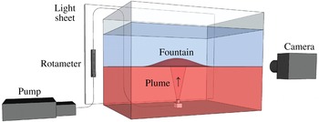
We carried out a series of experiments in a tank of dimension $40\times 40\times 50~\text{cm}$ (figure 1). The tank was filled with a layer of saline water (of depth $h_{l}$ and density $\unicode[STIX]{x1D70C}_{l}$ ), then a layer of fresh water (of density $\unicode[STIX]{x1D70C}_{u}$ and depth $h_{u}$ ) was supplied above this layer. To minimise any mixing, a sponge was placed on top of the layer of saline solution, and the fresh water was supplied very slowly to the sponge, from which the fresh water slowly spread out above the salt water. As seen in the photographs of the experiment (e.g. figure 2), the initial interface was very sharp, with any intermediate mixed layer being less than 1–2 mm in thickness. The layer of fresh water was filled to a depth $h_{u}$ . A source nozzle of diameter 4 mm was placed in the centre of its base, and a porous diffuser of size $1\times 1~\text{cm}$ was placed on this nozzle. Air was then supplied to the source nozzle with a flow rate $Q_{o}$ in the range $5{-}20~\text{cc}~\text{s}^{-1}$ using a peristaltic pump (Watson Marlow), leading to the production of a steady source of small bubbles from the top of the diffuser. As the bubbles rose from the air supply nozzle, a turbulent plume developed, entraining ambient fluid.

Figure 1.

Schematic of the experimental set-up.

Figure 2.

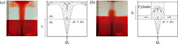
Images, from two experiments in which the plume reaches the interface, and then (a) continues upwards to the top of the tank, where the bubbles separate and the fluid mixes through the upper layer, or (b) forms a dense fountain above the interface and collapses back to the interface, forming an intermediate layer.

The tank was backlit using a light sheet (LightTape by Electro-LuminX Lighting Corp.). The lower layer of the fluid was dyed red while the upper layer remained clear. A series of mixtures of this red saline fluid and the fresh water, with intermediate salinity and dye concentration, were placed in the tank prior to the main experiment in order to generate a calibration curve to relate the degree of dilution of the saline water to the attenuation of light as recorded in a digital image of the tank using a NIKON D90 camera located on the opposite side of the tank to the light sheet. This calibration curve was then used to quantify the mixing in the tank produced by the fountain by analysing the evolution of the light intensity across the tank in a series of images taken at a frequency of 200 Hz during the main experiment (figure 1).

3 Observations of the plume in the lower layer

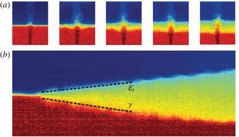
In the lower layer of the tank, a bubble plume was observed to develop, entraining ambient fluid and carrying it upwards (figure 2). As a result, a return flow in the ambient fluid developed, leading to a gradual descent of the top surface of the original lower layer fluid. By plotting a time series of a vertical line of pixels in the ambient fluid away from the plume, a descending front, $z=h_{d}(t)$ , can be seen. This corresponds to the so-called first-front observed in filling-box flows (Baines & Turner Reference Baines and Turner1969). By measuring the initial rate of descent of this front, $\text{d}h_{d}/\text{d}t$ , in a tank with cross-sectional area $A$ , the upward volume flux in the plume,  $Q(t)$ , can be estimated by the balance

(3.1) $$\begin{eqnarray}A\frac{\text{d}h_{d}}{\text{d}t}=-Q.\end{eqnarray}$$

We may quantify the buoyancy flux in the plume in terms of the source buoyancy flux $gQ_{b}$ , where $g$ is the acceleration due to gravity and $Q_{b}$ is the source bubble flux. If the plume behaves as a single-phase plume with buoyancy flux $B$ , we expect that the volume flux at height $z$ above the source of bubbles is

(3.2) $$\begin{eqnarray}Q(z)=\unicode[STIX]{x1D6FE}B^{1/3}(z_{o}+z)^{5/3},\end{eqnarray}$$

where $z_{o}$ is the virtual origin and $\unicode[STIX]{x1D6FE}$ is a constant, of value $0.15\pm 0.01$ , related to the entrainment coefficient $\unicode[STIX]{x1D6FC}$ by the relation $\unicode[STIX]{x1D6FE}=(6\unicode[STIX]{x1D6FC}/5)(9\unicode[STIX]{x1D6FC}/10)^{1/3}$ for a classical single-phase plume (Morton, Taylor & Turner Reference Morton, Taylor and Turner1956). 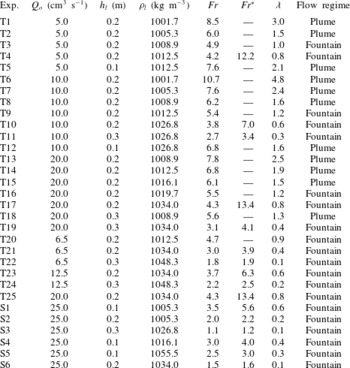By combining (3.1) and (3.2), with $z=h_{d}$ , we can estimate $\unicode[STIX]{x1D6FE}$ for all of the experiments listed in table 1, and we find that $\unicode[STIX]{x1D6FE}=0.16\pm 0.03$ . This is consistent with the classical value for a turbulent buoyant plume, suggesting that the assumption that the plume behaves as a single-phase plume in the lower layer is a reasonable approximation (figure 3). In estimating $\unicode[STIX]{x1D6FE}$ , we estimated the virtual origin of the plume in the lower layer by estimating the location of the equivalent point source for the linearly spreading plume, given that, from plume theory, the radius of the plume follows a law of the form $r=6\unicode[STIX]{x1D6FC}/5(z_{o}+z)$ . This suggests that $z_{o}\approx 2~\text{cm}$ in our experiments. We note that near the actual source, the flow involves a relatively large flux of gas, but as the flow mixes with water and dilutes, the gas volume fraction decreases so that, for points 10–15 cm above the source, it has fallen to values less than 0.05, and the flow has adjusted to that of a classical Boussinesq plume. The estimate of the virtual origin implicitly accounts for this adjustment process near the source, representing the plume flow at the interface in terms of that produced from an idealised point source with the same buoyancy flux.

Figure 3.

(a) Series of images indicating how the fountain mixes across the interface. The colour denotes the horizontally averaged salinity at each point in the tank, and indicates the gradual formation of intermediate density fluid at the interface. (b) Time series (horizontal) of a vertical line through the ambient fluid away from the fountain. The gradual descent of the base of the intermediate layer into the original lower layer can be used to quantify the flux of lower layer fluid which is entrained into the plume and carried into the fountain. The gradual ascent of the mixed layer can be used to quantify the rate of mixing of upper layer fluid into the collapsing fountain.

Table 1.

Range of experimental conditions in the bubble plumes. The label T denotes two-phase bubble plume experiments, while the label S denotes single-phase experiments.

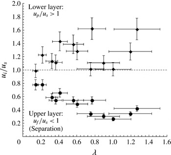
If the bubble rise speed is smaller than the plume speed in the lower layer, we expect that the flow may be approximated as a single-phase flow. To this end, we have measured the size of the bubbles produced from the nozzle used in our experiments by using high-precision analysis of the images from the experiments, and find values in the range 0.1–0.2 cm. Bubbles in this size range rising in water are ellipsoidal, and there are extensive experimental data showing that such bubbles in fact have an approximately constant rise speed of $0.23~\text{m}~\text{s}^{-1}$ (Clift, Grace & Weber Reference Clift, Grace and Weber1978). As a further check, we made independent measurements of the bubble rise speed using our high-frequency images of the experiments to track the speed of individual bubbles, and this also confirms the bubble rise speeds were in the range $0.23\pm 0.01~\text{m}~\text{s}^{-1}$ . To estimate the horizontally averaged ‘top-hat’ rise speed of the fluid in the plume (cf. Morton et al. Reference Morton, Taylor and Turner1956) we use single-phase plume theory, which predicts that

(3.3) $$\begin{eqnarray}u=kB^{1/3}(z_{o}+z)^{-1/3},\end{eqnarray}$$

where $k=(5/6\unicode[STIX]{x1D6FC})(9\unicode[STIX]{x1D6FC}/10)^{1/3}\approx 3.84$ . Substituting in the values from our experiments, we find that at the initial position of the interface between the lower and upper layers, $z=h_{l}$ , the plume speed is larger than the rise speed of the bubbles for each experiment (diamonds, figure 4), and so we expect that the motion in the lower layer may be approximated as a single-phase plume, and that the scaling law (3.2) applies, consistent with our measurements (cf. figure 3).

Figure 4.

Rise speed of the fluid in the plume as a fraction of the rise speed of the bubbles (diamonds), and also the rise speed of the fluid in the fountain as a fraction of the rise speed of the bubbles (circles). Both quantities are shown as functions of the ratio of the buoyancy of the plume relative to the lower layer and the buoyancy of the upper layer relative to the lower layer, $\unicode[STIX]{x1D706}$ . If $\unicode[STIX]{x1D706}<1$ , then on entering the upper layer the bulk density of the flow is in excess of the density of the upper layer, and the flow then evolves as a fountain in the upper layer.

4 Condition for fountain development in the upper layer

Given the model for the motion of the plume in the lower layer, we can estimate the bulk density of the plume on reaching the initial position of the interface, $z=h_{l}$ , by using the conservation of buoyancy flux, which is equivalent to the conservation of gas flux in the lower layer. Given the relationship between the plume buoyancy $g^{\prime }$ , volume flux $Q$ and buoyancy flux $B$ , $g^{\prime }Q=B$ , we expect that at $z=h_{l}$ ,

(4.1) $$\begin{eqnarray}g_{l}^{\prime }(h_{l})=\frac{B^{2/3}}{\unicode[STIX]{x1D6FE}(z_{o}+h_{l})^{5/3}},\end{eqnarray}$$

where $g_{l}^{\prime }(h_{l})=g(\unicode[STIX]{x1D70C}_{l}(h_{l})-\unicode[STIX]{x1D70C}(h_{l}))/\unicode[STIX]{x1D70C}_{l0}$ is the buoyancy of the plume fluid relative to the lower layer, at the interface, and $\unicode[STIX]{x1D70C}_{l0}$ is a reference density, taken to be that of fresh water. On passing into the upper layer of the experimental reservoir, the buoyancy changes by the buoyancy difference between the upper and lower layer, $g_{ul}^{\prime }=g_{l}^{\prime }(h_{l})-g_{u}^{\prime }(h_{l})=g(\unicode[STIX]{x1D70C}_{l}(h_{l})-\unicode[STIX]{x1D70C}_{u}(h_{l}))/\unicode[STIX]{x1D70C}_{l0}$ say, and so the buoyancy relative to the upper layer of the rising bubble–water mixture, which has density $\unicode[STIX]{x1D70C}(h_{l})$ at the interface, is given by $g_{u}^{\prime }(h_{l})=g(\unicode[STIX]{x1D70C}_{u}(h_{l})-\unicode[STIX]{x1D70C}(h_{l}))/\unicode[STIX]{x1D70C}_{l0}$ . This may be expressed as

(4.2) $$\begin{eqnarray}g_{u}^{\prime }(h_{l})=g_{l}^{\prime }(h_{l})-g_{ul}^{\prime }=g_{ul}^{\prime }[\unicode[STIX]{x1D706}-1],\end{eqnarray}$$

where $\unicode[STIX]{x1D706}=g_{l}^{\prime }(h_{l})/g_{ul}^{\prime }(h_{l})$ . Equation (4.2) expresses the relation between the buoyancy of the flow above and below the interface and the buoyancy difference across the interface of the two liquid layers.

It follows that if $\unicode[STIX]{x1D706}>1$ then the plume fluid is still buoyant above the interface. If the continuing plume speed in the upper layer remains larger than the bubble rise speed, then we expect the plume to rise to the top of the tank (see figure 2 a). However, we note that if the tank is very tall, then as the plume continues to rise through the upper layer, the plume speed will decrease and eventually the bubbles can separate from the fluid, leading to collapse of the remaining relatively saline fluid and formation of a fountain.

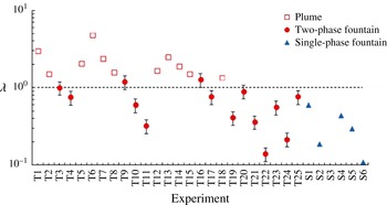
In contrast, if $\unicode[STIX]{x1D706}<1$ , we expect the plume to transition into a collapsing fountain above the interface (cf. Kumagai Reference Kumagai1984), with the additional complexity that the bubbles then separate from this fountain and carry on rising to the top of the tank (see figure 2 b). In figure 5, we present the estimated value of $\unicode[STIX]{x1D706}$ for each of the experiments listed in table 1. If the flow developed into a fountain, we use solid symbols, whereas in the case that the flow reached the top of the tank, we use open symbols. The figure shows very good agreement of the predicted transition, $\unicode[STIX]{x1D706}=1$ , with the observed transition in the behaviour of each of the flows.

Figure 5.

Comparison of the value of $\unicode[STIX]{x1D706}$ estimated for each of the experiments listed in table 1, with the observation of whether the experiment leads to a collapsing fountain (closed symbols) or a flow which reached the surface of the reservoir (open symbols).

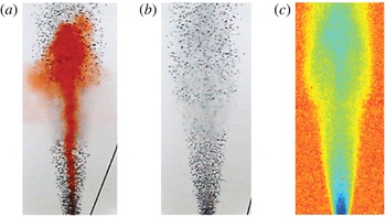
Henceforth, our main focus lies in flows for which $\unicode[STIX]{x1D706}<1$ . In this case there is a transition to fountaining behaviour in the upper layer. Our experimental observations show that the fluid bubble mixture rises above the interface and that the fluid then comes to rest some distance above the interface, while the bubbles continue to rise. To help clarify the motion of the fluid and the bubbles, in figure 6(a) we present a photograph of the bubble–water mixture. In this figure, it may be seen how the lower layer fluid rises a certain distance above the interface, where it then comes to rest and falls back to the interface, mixing with some of the upper layer fluid en route. In figure 6(b) we present an image with no dye in the fluid, which illustrates the rise of the bubbles in both the lower layer, where they gradually spread out as predicted by the plume model, and in the upper layer, where they rise in a nearly cylindrical region above the interface with no significant change in radius with height. This zone in which the bubbles rise is illustrated more clearly in figure 6(c) using a false colour scheme for emphasis.

Figure 6.

Images illustrating: (a) the case in which some of the fluid carried up from the lower layer is dyed red, showing how it rises a finite distance then collapses back to the interface; (b) bubbles rising in the plume below the interface and the fountain above the interface; and (c) a time-lapse image to visualise the spatial distribution of the bubbles averaged over time, in both the plume, below the interface, and the fountain, above the interface.

Figure 7.

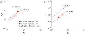
Variation of (a) the height of rise of the fountain and (b) the entrainment coefficient, as a function of the Froude number. Data are shown for the bubble fountains using the Froude number $Fr$ , based on the density difference between the saline and fresh fluid (solid circular symbols, (5.2)), and using the Froude number $Fr^{\ast }$ , based on the bulk density difference between the upper layer fluid and the bulk plume fluid (open circular symbols, (5.1)). Also shown in the figure are data from a series of purely single-phase experiments using fresh and saline water, shown with the blue triangular symbols, based on the Froude number $Fr_{s}$ .

5 Height of rise and entrainment in the fountains

We have measured the height of rise of the dense fluid in the fountain and also the rate of entrainment of upper layer fluid into the fountain, by estimating the rate of ascent of the mixed layer above the interface, as shown in figure 3. In order to understand the control of each of these properties, it is useful to calculate the Froude number of the fountain, the square of which may be regarded as a measure of the ratio of the kinetic energy of the fluid in the fountain and the potential energy required to lift the fluid in the fountain a vertical distance comparable to the radius of the fountain. In defining the Froude number, there are two possible models for the buoyancy of the fountain fluid. We might consider the bulk buoyancy of the fluid, which includes the presence of the bubbles. However, on inspection of the image in figure 6 and other observations of the fountain, it is clear that the bubbles separate from the fountain liquid, and produce a region in which the bubbles rise through both the fountain liquid and the surrounding upper layer fluid. Indeed, we can estimate the characteristic speed of the fountain, based on the buoyancy and momentum flux of the fluid rising from the interface, by using the scaling for the horizontally averaged ‘top-hat’ fountain speed at the initial position of the interface (Turner Reference Turner1966), $u_{l}=M^{3/4}/B^{1/2}$ , where $M=u_{l}Q$ and $B=g_{u}^{\prime }Q$ , with $Q$ evaluated at the interface. If we compare this speed with the rise speed of the bubbles we find that for all our experiments the rise speed of the bubbles is greater than the speed of the fountain (figure 4), and so we expect the bubbles to separate from the fountain fluid, as is indeed observed (figure 6). As a result, it may be more appropriate to define the Froude number in terms of the density difference between the lower layer and upper layer fluids. In figure 7(a) we illustrate the height of rise of the fountain in the upper layer, $h_{i}$ , as a function of (i) a Froude number $Fr^{\ast }$ based on the difference between the plume bulk density at the interface, $z=h_{l}$ , and the upper layer, $Fr^{\ast }$ shown by open circles and defined as

(5.1) $$\begin{eqnarray}Fr^{\ast }=\frac{u_{l}}{(g_{u}^{\prime }(h_{l})r(h_{l}))^{1/2}}\end{eqnarray}$$

and (ii) a Froude number $Fr$ based on the density difference between the upper and lower layer fluid, shown by closed circles and defined by

(5.2) $$\begin{eqnarray}Fr=\frac{u_{l}}{(g_{ul}^{\prime }r(h_{l}))^{1/2}},\end{eqnarray}$$

where $r(h_{l})$ is the radius of the plume at the interface, given by $r(h_{l})=6\unicode[STIX]{x1D6FC}/5(h_{l}+z_{o})$ and $u_{l}$ is the plume speed at the interface (3.3).

In figure 7(a), we also present the fountain heights above the interface, $h_{i}$ , obtained from a series of reference single-phase experiments we have carried out using fresh and saline fluid (shown by blue triangles). These experiments use a Froude number $Fr_{s}$ based on the density difference between the plume fluid at the interface and the upper layer fluid. It is seen that the height of the single-phase fountains (triangles) and bubble fountains (solid circles) depend on Froude number according to the relations

(5.3a,b ) $$\begin{eqnarray}h_{i}=(0.63\pm 0.08)Fr_{s}^{2}r(h_{l})\quad \text{and}\quad h_{i}=(0.33\pm 0.05)Fr^{2}r(h_{l}),\end{eqnarray}$$

with the Froude number varying from 1–7. In contrast if we do apply the bulk buoyancy difference in our definition of the Froude number for the bubble fountains, $Fr^{\ast }$ , we find a relation $h_{i}=(0.42\pm 0.15)r(h_{l})Fr^{\ast }$ (open circles) with the Froude number, $Fr^{\ast }$ , now lying in the range 2–10. This has much more scatter than the fit (5.3b ) using the Froude number $Fr$ (5.2). In these expressions, $r(h_{l})$ is the radius of the fountain at the initial position of the interface between the fresh and saline fluid.

An original aim of the experimental study was to determine the rate of mixing of the upper layer fluid into the fountain. We have measured this for each of the experiments by calculating the rate of ascent of the mixed layer above the interface, located at $z=h_{m}$ (cf. figure 3). We then define an entrainment coefficient $E_{i}$ according to the relation

(5.4) $$\begin{eqnarray}A\frac{\text{d}h_{m}}{\text{d}t}=E_{i}Q(h_{m}),\end{eqnarray}$$

where $Q(h_{m})$ is the plume volume flux at this upper interface. In figure 7(b), we illustrate the calculated value of $E_{i}$ as a function of $Fr$ and also $Fr^{\ast }$ for each of our bubble fountain experiments, and also for the single-phase salt–freshwater experiments as a function of $Fr_{s}$ . The value of $\text{d}h_{m}/\text{d}t$ is found during the initial stages of the experiment (cf. figure 3). It is seen that, for the bubble fountain and the saline fountain, $E_{i}$ follows the trend

(5.5a,b ) $$\begin{eqnarray}E_{i}=(0.05\pm 0.02)Fr^{2}\quad \text{and}\quad E_{i}\sim (0.27\pm 0.09)Fr_{s}^{2}.\end{eqnarray}$$

This has the same dependence on $Fr$ as the fountain height (5.2), and this is consistent with a picture in which the entrainment occurs around the flanks of the fountain, so that the total entrainment increases with the fountain height. Again, the collapse of the bubble plume data for $E_{i}$ using $Fr$ (solid circles) is more compelling than that using the Froude number $Fr^{\ast }$ (open circles).

Our results for the height of rise of the single-phase fountain are consistent with data presented by Hunt & Burridge (Reference Hunt and Burridge2015), who found the relation $h_{i}=0.82Fr_{s}^{2}r_{n}$ for the height of rise of a single-phase fountain issuing into a uniform layer from a source, where $r_{n}$ is the size of the source nozzle. However, the constant of proportionality 0.82 is larger than in our experiments (5.3a ). We suggest that this difference is the result of the different radial distribution of momentum and buoyancy in the fluid supplied to the fountain from the turbulent plume in the lower layer compared to the flow being supplied from a nozzle as in the Burridge & Hunt experiments. Also, our single-phase fountain entrainment law is directly analogous to the results of Cardoso & Woods (Reference Cardoso and Woods1993), who found a constant of proportionality 0.25 for a single-phase plume entraining across an interface into a density-stratified fluid. It is worth noting, for reference, that data presented by Baines (Reference Baines1975) for the entrainment into a single-phase fountain followed a scaling $Fr_{s}^{3}$ , but this was for smaller values of the Froude number than reported in the present work. In a study of a ventilation flow, Lin & Linden (Reference Lin and Linden2005) found that the entrainment coefficient $E_{i}$ for a single-phase fountain had value $0.65\pm 0.1$ for Froude numbers, which we estimate from their data fell within the range 1–2; this is consistent with our saline fountain data for Froude numbers in the range 1.25–1.75 (5.5b ). For clarity, we note that when using the entrainment model for a single-phase fountain, we use the density contrast between the fountain fluid and the layer being entrained to define the Froude number.