2.1 Jackson’s model

The starting point of our derivation is the same as in Bouchut et al. (Reference Bouchut, Fernández-Nieto, Mangeney and Narbona-Reina2015), i.e. the 3D model proposed by Jackson (Reference Jackson2000) for flows of solid granular materials filled (saturated) with fluid. A related theory of mixtures is also developed in Brenner (Reference Brenner2009). The two mass conservation equations for the solid and fluid phases are respectively

and the equations of momentum conservation for each phase are The velocities are $\boldsymbol{v}$ for the solid phase and $\boldsymbol{u}$ for the fluid phase, while $\unicode[STIX]{x1D64F}_{s}$ and $\unicode[STIX]{x1D64F}_{f_{m}}$ denote the (symmetric) stress tensors for the solid and the fluid respectively. Moreover, the constant densities are denoted by ${\it\rho}_{s}$ and ${\it\rho}_{f}$ . Acceleration due to gravity is denoted by $\boldsymbol{g},$ and $\boldsymbol{f}_{0}$ represents the average value of the resultant force exerted by the fluid on a solid particle. The solid volume fraction is ${\it\varphi}$ . The combination of (2.1a ) and (2.1b ) yields the mass conservation for the mixture,

where

are the density and velocity of the mixture respectively. Dividing (2.1a ) by ${\it\rho}_{s}$ , (2.1b ) by ${\it\rho}_{f}$ and adding the results gives

which can also be written as $\boldsymbol{{\rm\nabla}}\boldsymbol{\cdot }\boldsymbol{v}=\boldsymbol{{\rm\nabla}}\boldsymbol{\cdot }((1-{\it\varphi})(\boldsymbol{v}-\boldsymbol{u}))$ . It should be noted that this relation does not imply that $\boldsymbol{{\rm\nabla}}\boldsymbol{\cdot }\boldsymbol{V}_{m}$ is equal to zero.

According to Anderson & Jackson (Reference Anderson and Jackson1967) and as in Bouchut et al. (Reference Bouchut, Fernández-Nieto, Mangeney and Narbona-Reina2015), the force $\boldsymbol{f}_{0}$ is decomposed into the sum of the buoyancy force $\boldsymbol{f}_{B}$ and all remaining contributions $\boldsymbol{f}$ ,

where $p_{f_{m}}$ is the fluid pressure in the mixture (pore pressure). The term $\boldsymbol{f}$ combines the drag force, the lift force and the virtual mass force. It should be noted that separation of the buoyancy force from the rest of inter-phase forces is not trivial, as explained in Jackson (Reference Jackson2000). Here, we assume that $\boldsymbol{f}$ can be expressed simply by the drag force, thus

$\tilde{{\it\beta}}$ being the drag coefficient given as in Pailha & Pouliquen (Reference Pailha and Pouliquen2009) and Iverson & George (Reference Iverson and George2014) by

where ${\it\eta}_{f}$ is the dynamic viscosity of the fluid and ${\it\kappa}$ is the hydraulic permeability of the granular aggregate, which depends on ${\it\varphi}$ .

By substituting (2.6) into (2.2a ) and (2.2b ), we obtain

It should be noted that adding (2.9a ) and (2.9b ) and taking into account (2.1a ), (2.1b ) yields the conservation of total momentum

We shall assume rheologies of the form

where $p_{s}$ and $p_{f_{m}}$ are the total pressures for the solid and fluid within the mixture respectively and $\widetilde{\unicode[STIX]{x1D64F}}_{s}$ , $\widetilde{\unicode[STIX]{x1D64F}_{f_{m}}}$ need to be defined, according to rheological assumptions. With (2.11), the fluid momentum equation (2.9b ) involves the pressure contribution $-(1-{\it\varphi})\boldsymbol{{\rm\nabla}}p_{f_{m}}$ . It is important to see that, since the factor $1-{\it\varphi}$ appears also on the left-hand side, the velocity $\boldsymbol{u}$ , however, only feels the term $-\boldsymbol{{\rm\nabla}}p_{f_{m}}$ , as expected since $p_{f_{m}}$ is the pore pressure. The interpretation of the solid momentum equation (2.9a ) is that the solid feels the buoyancy term $-{\it\varphi}\boldsymbol{{\rm\nabla}}p_{f_{m}}$ and the solid pressure term $-\boldsymbol{{\rm\nabla}}p_{s}$ . The latter pressure $p_{s}$ (also called effective normal stress) represents only the effects of grain interactions, and its gradient can be evaluated in practice by measuring the force exerted on a grid immersed into the mixture.

The system of eight scalar equations (2.1a,b ), (2.9a,b ) has nine scalar unknowns ${\it\varphi}$ , $p_{s}$ , $p_{f_{m}}$ , and the components of $\boldsymbol{u}$ and $\boldsymbol{v}$ . Thus, as exposed in Bouchut et al. (Reference Bouchut, Fernández-Nieto, Mangeney and Narbona-Reina2015), it is not closed, and this is due to the averaging process used for its deduction (see Jackson Reference Jackson2000 for details). Therefore, a closure relation is needed, under the form of an additional scalar equation that should be imposed, based on the physical processes involved. A possible closure is to impose the incompressibility of the solid phase, $\boldsymbol{{\rm\nabla}}\boldsymbol{\cdot }\boldsymbol{v}=0$ , considered in the previous work (Bouchut et al. Reference Bouchut, Fernández-Nieto, Mangeney and Narbona-Reina2015). However, in real granular materials the dilatancy effects, due to geometrical congestion, may induce changes of the solid dilation rate $\boldsymbol{{\rm\nabla}}\boldsymbol{\cdot }\boldsymbol{v}$ , even if the mass of the granular material remains constant. This effect has to be included in the model instead of incompressibility.

2.2 Closure and energy balance

The energy balance associated with Jackson’s system can be written, as in Bouchut et al. (Reference Bouchut, Fernández-Nieto, Mangeney and Narbona-Reina2015), as

where $X$ denotes the space position. The friction effects naturally give a dissipative term $\boldsymbol{f}\boldsymbol{\cdot }(\boldsymbol{v}-\boldsymbol{u})\leqslant 0$ , and it is also natural to assume that $\widetilde{\unicode[STIX]{x1D64F}_{f_{m}}}:\,\boldsymbol{{\rm\nabla}}\boldsymbol{u}\leqslant 0$ . The sign of $\unicode[STIX]{x1D64F}_{s}:\boldsymbol{{\rm\nabla}}\boldsymbol{v}$ remains, however, undetermined. Since by (2.11)

and it is also natural to have $\widetilde{\unicode[STIX]{x1D64F}}_{s}:\boldsymbol{{\rm\nabla}}\boldsymbol{v}\leqslant 0$ , the term $p_{s}\boldsymbol{{\rm\nabla}}\boldsymbol{\cdot }\boldsymbol{v}$ remains. As mentioned above, the closure relation that states the incompressibility of the solid phase $\boldsymbol{{\rm\nabla}}\boldsymbol{\cdot }\boldsymbol{v}=0$ gives a consistent energy balance and the model of Bouchut et al. (Reference Bouchut, Fernández-Nieto, Mangeney and Narbona-Reina2015), but does not take into account dilatancy. Thus, we consider the following closure equation to Jackson’s model, involving the solid dilation rate $\boldsymbol{{\rm\nabla}}\boldsymbol{\cdot }\boldsymbol{v}$ :

with ${\it\Phi}$ a function to be determined, which may depend on the unknowns of the system, as discussed in the next subsection. This kind of ‘weakly compressible’ closure is considered in low-Mach-number flows, see, for example, Penel, Dellacherie & Després (Reference Penel, Dellacherie and Després2015). This equation (2.14) together with (2.1a , b ), (2.9a , b ) (and (2.11) with suitable definitions of $\widetilde{\unicode[STIX]{x1D64F}}_{s}$ , $\widetilde{\unicode[STIX]{x1D64F}_{f_{m}}}$ ), gives a closed system. Then, on the right-hand side of (2.12) with the decomposition (2.13), only the first term $p_{s}{\it\Phi}$ is not always non-positive. This term is further analysed in § 2.4.

2.3 Dilatancy in dense granular flows

In the work of Roux & Radjai (Reference Roux, Radjai and Herrmann1998), a model for introducing dilatancy effects into the behaviour of dry granular media is proposed. This effect is directly related to the changes experienced by the solid volume fraction. In particular, the rate of volume change is given by $\dot{{\it\gamma}}\tan {\it\psi}$ , where $\dot{{\it\gamma}}=|D\boldsymbol{v}|$ is the norm of the strain rate $D\boldsymbol{v}=(\boldsymbol{{\rm\nabla}}\boldsymbol{v}+\boldsymbol{{\rm\nabla}}\boldsymbol{v}^{t})/2$ , and ${\it\psi}$ is the so-called ‘dilation angle’. This means more explicitly that

From the mass equation (2.1a ) we have $\partial _{t}{\it\varphi}+\boldsymbol{v}\boldsymbol{\cdot }\boldsymbol{{\rm\nabla}}{\it\varphi}=-{\it\varphi}\,\boldsymbol{{\rm\nabla}}\boldsymbol{\cdot }\boldsymbol{v}$ , thus we can reformulate (2.15) as a relation between the solid dilation rate $\boldsymbol{{\rm\nabla}}\boldsymbol{\cdot }\boldsymbol{v}$ and the dilation angle ${\it\psi}$ , as

The dilation angle ${\it\psi}$ is in turn related to the solid volume fraction ${\it\varphi}$ , and a linear approximation can be written as ${\it\psi}=a({\it\varphi}-{\it\varphi}_{c}^{eq})$ , with $a>0$ , and ${\it\varphi}_{c}^{eq}$ the critical-state equilibrium compacity, which corresponds to the volume fraction obtained when a steady-state regime is reached (Schofield & Wroth Reference Schofield and Wroth1968; Wood Reference Wood1990). This critical-state compacity ${\it\varphi}_{c}^{eq}$ is generally a function of the solid pressure $p_{s}$ , of the shear rate $\dot{{\it\gamma}}$ and of the granular temperature, increasing with respect to $p_{s}$ . For the case of pores filled by fluid considered here, the granular temperature can be neglected. For steady granular flows it was shown in GDR MiDi group (2004), Cassar, Nicolas & Pouliquen (Reference Cassar, Nicolas and Pouliquen2005), Da Cruz et al. (Reference Da Cruz, Emam, Prochnow, Roux and Chevoir2005) and Forterre & Pouliquen (Reference Forterre and Pouliquen2008) that ${\it\varphi}_{c}^{eq}$ is indeed a decreasing function of $\dot{{\it\gamma}}/\sqrt{p_{s}}$ in the dry case (respectively of $\dot{{\it\gamma}}/p_{s}$ in the wet case).

This approach with critical-state compacity ${\it\varphi}_{c}^{eq}$ allows us to recover the different behaviours of loose and dense granular media, according to the sign of ${\it\varphi}-{\it\varphi}_{c}^{eq}$ . Namely, for a dense packing ${\it\varphi}>{\it\varphi}_{c}^{eq}$ , one has a positive dilation angle, ${\it\psi}>0$ , which induces dilation of the granular medium, $\boldsymbol{{\rm\nabla}}\boldsymbol{\cdot }\boldsymbol{v}>0$ , while for a loose packing ${\it\varphi}<{\it\varphi}_{c}^{eq}$ , one has a negative dilation angle, ${\it\psi}<0$ , which induces contraction of the granular medium, $\boldsymbol{{\rm\nabla}}\boldsymbol{\cdot }\boldsymbol{v}<0$ . This is valid as soon as $\dot{{\it\gamma}}>0$ , i.e. when a deformation occurs.

Pailha & Pouliquen (Reference Pailha and Pouliquen2009) deal with the immersed granular flow system. They consider the preceding model where a linearization of $\tan {\it\psi}$ is proposed,

$K>0$ being a calibration constant (dilation constant). We adopt this dilation model to write

Thus, the closure considered in this work for (2.14) is

As exposed by Iverson (Reference Iverson2005) and Schaeffer & Iverson (Reference Schaeffer and Iverson2008), there is a coupling between the dilatancy and the pore pressure, called ‘pore pressure feedback’. This effect plays an important role in the way a landslide starts, and then dramatically affects the flow dynamics. The formula (2.18) reproduces the contraction–dilation effects well (see Pailha & Pouliquen Reference Pailha and Pouliquen2009; Andreotti, Forterre & Pouliquen Reference Andreotti, Forterre and Pouliquen2011), which are the following.

1. (i) If ${\it\varphi}>{\it\varphi}_{c}^{eq}$ then the granular medium dilates ( $\boldsymbol{{\rm\nabla}}\boldsymbol{\cdot }\boldsymbol{v}>0$ ) as soon as there is a deformation ( $\dot{{\it\gamma}}>0$ ). Consequently,

   1. (1) the fluid must be sucked into the mixture,

   2. (2) the pore pressure decreases.

2. (ii) If ${\it\varphi}<{\it\varphi}_{c}^{eq}$ then the granular medium contracts ( $\boldsymbol{{\rm\nabla}}\boldsymbol{\cdot }\boldsymbol{v}<0$ ) as soon as there is a deformation ( $\dot{{\it\gamma}}>0$ ). Consequently,

   1. (1) the fluid must be expelled from the mixture,

   2. (2) the pore pressure increases.

The type of closure (2.18) entails a modification of the coefficient of the Coulomb friction law which becomes $\tan ({\it\delta}+{\it\psi})$ instead of $\tan {\it\delta}$ . By linearization, we can write an effective friction coefficient as

In the thin-layer expansion performed below, we neglect the deviatoric solid stress $\widetilde{\unicode[STIX]{x1D64F}}_{s}$ inside the mixture, and only consider the bottom solid friction with the friction coefficient $\tan {\it\delta}_{eff}$ .

Closure laws slightly different from (2.19) are considered in § 4.6.

2.4 Interpretation as a compressible model

We would like here to propose an interpretation of the Roux & Radjai (Reference Roux, Radjai and Herrmann1998) dilatancy relation under the form (2.18) as a compressible model, which enables us to write down a fully dissipative energy equation in the case when the critical-state compacity ${\it\varphi}_{c}^{eq}$ depends only on the pressure $p_{s}$ , and not on $\dot{{\it\gamma}}$ .

We consider the critical volume fraction ${\it\varphi}_{c}^{eq}$ to be an increasing function of the solid pressure only, ${\it\varphi}_{c}^{eq}={\it\varphi}_{c}^{eq}(p_{s})$ , bounded by some maximal value ${\it\varphi}_{max}$ ( ${\it\varphi}_{max}\sim 0.6$ for monodisperse spherical grains, but ${\it\varphi}_{max}$ can be higher for real polydisperse materials). This function ${\it\varphi}={\it\varphi}_{c}^{eq}(p_{s})$ can be defined by its inverse $p=p_{c}^{eq}({\it\varphi})$ ( $p_{c}^{eq}({\it\varphi})$ being called the critical pressure), as for example $p_{c}^{eq}({\it\varphi})=\mathscr{K}{\it\varphi}^{{\it\gamma}}/({\it\varphi}_{max}-{\it\varphi})^{{\it\iota}}$ , for some coefficient $\mathscr{K}$ , and some exponents ${\it\gamma}$ , ${\it\iota}$ . Particular dependences of $p_{c}^{eq}({\it\varphi})$ in ${\it\varphi}$ appear for example in Lee, Huang & Chiew (Reference Lee, Huang and Chiew2015). Since the granular temperature is negligible in the present context of pores filled by fluid, the critical pressure $p_{c}^{eq}({\it\varphi})$ is only related to the deformation of the grains that are in contact. A formula valid in the context of granular mixtures is given in Iverson & George (Reference Iverson and George2014) as $p_{c}^{eq}({\it\varphi})/p_{0}=\exp (({\it\varphi}-{\it\varphi}_{min})/a)-1$ , with $0.01\leqslant a\leqslant 0.05$ and $10~\text{Pa}\leqslant p_{0}\leqslant 1000~\text{Pa}$ , depending on the materials.

Classically, in thermodynamics, the mechanical internal energy $U$ is related to the pressure $p$ and volume $V$ by the relation $\text{d}U=-p\,\text{d}V$ . Here, the specific volume (i.e. volume per mass unit) is $1/({\it\rho}_{s}{\it\varphi})$ , thus with the critical pressure $p_{c}^{eq}({\it\varphi})$ one can associate by this relation a specific internal energy (i.e. internal energy per mass unit) $e_{c}^{eq}({\it\varphi})$ . Since $\text{d}(1/{\it\varphi})=-\text{d}{\it\varphi}/{\it\varphi}^{2}$ we obtain the differential relation

Then, writing the mass equation (2.1a ) as $\partial _{t}{\it\varphi}+\boldsymbol{v}\boldsymbol{\cdot }\boldsymbol{{\rm\nabla}}{\it\varphi}+{\it\varphi}\boldsymbol{{\rm\nabla}}\boldsymbol{\cdot }\boldsymbol{v}=0$ , and multiplying it by $\text{d}\text{e}_{c}^{eq}/\text{d}{\it\varphi}$ , we obtain

Multiplying this by ${\it\varphi}$ and using again (2.1a ) yields

Adding this times ${\it\rho}_{s}$ to the energy equation (2.12) gives

Now, according to (2.18) and since $p_{s}-p_{c}^{eq}({\it\varphi})$ and ${\it\varphi}-{\it\varphi}_{c}^{eq}(p_{s})$ have opposite signs because ${\it\varphi}_{c}^{eq}$ is an increasing function of $p_{s}$ , one has $(p_{s}-p_{c}^{eq})\boldsymbol{{\rm\nabla}}\boldsymbol{\cdot }\boldsymbol{v}\leqslant 0$ , and the energy balance equation (2.24) has a non-positive right-hand side. This means that, as required by the laws of physics, the total mechanical energy of the system is dissipated.

Another way to understand the dilatancy law (2.18) is to perform a further linear approximation $K({\it\varphi}-{\it\varphi}_{c}^{eq}(p_{s}))\simeq K_{p}(p_{c}^{eq}({\it\varphi})-p_{s})$ , which is valid for ${\it\varphi}$ and $p_{s}$ far from extreme values $0,{\it\varphi}_{max}$ and $0,\infty$ respectively, with $K_{p}$ the order of magnitude of $K(\text{d}p_{c}^{eq}/\text{d}{\it\varphi})^{-1}$ . Then, the dilatancy law (2.18) is transformed into

which can be written also as

When (2.26) is introduced into the stress in (2.9a ) it gives a diffusion equation on the solid velocity $\boldsymbol{v}$ (or on its divergence), with a diffusion coefficient that is induced by the Roux–Radjai dilatancy law,

Indeed, (2.26) appears clearly as a compressible rheological law with bulk viscoplastic term (because of $\dot{{\it\gamma}}$ in the denominator), which can be compared with (6) in Lee et al. (Reference Lee, Huang and Chiew2015).

We can propose also a general closure law under the form of a critical pressure $p_{c}^{eq}({\it\varphi},\dot{{\it\gamma}})$ that generalizes (2.25), by defining ${\it\Phi}$ in (2.14) as

where $p_{compr}({\it\varphi})$ is a static compressible law, and $I_{eq}({\it\varphi})$ is an equilibrium relating the volume fraction ${\it\varphi}$ to the inertial number $I$ . It can be, for example, $I_{eq}({\it\varphi})=(\bar{{\it\varphi}}_{c}^{stat}-{\it\varphi})/K_{2}$ in the context of (5.8). The compressible pressure $p_{compr}$ can be taken as above, $p_{compr}({\it\varphi})/p_{0}=\exp (({\it\varphi}-{\it\varphi}_{min})/a)-1$ .

2.5 Domain and boundary conditions

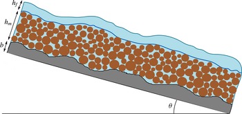
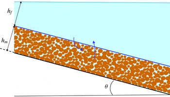
We assume that the mixture ( $0<{\it\varphi}<1$ ) lies between a fixed bottom and an interface, and that between the interface and an upper free surface there is only fluid ( ${\it\varphi}\equiv 0$ ), see figure 1. The thickness of the mixture layer is denoted by $h_{m}$ , the thickness of the fluid-only layer by $h_{f}$ , and the fixed bottom is defined by a function $b$ .

Figure 1.

Domain and geometrical parameters. The solid–fluid mixture lies between a fixed bottom and an upper pure fluid layer. The width $h_{m}$ of the mixture layer and the width $h_{f}$ of the pure fluid layer evolve with time.

The fluid velocity in the top layer is denoted by $\boldsymbol{u}_{f}$ , and in the mixture layer by  $\boldsymbol{u}$ , while $\boldsymbol{v}$ denotes the velocity of the solid phase. For other terms, we will use as general notation the subscript $()_{s}$ for the solid phase, $()_{f_{m}}$ for the fluid in the mixture and just $()_{f}$ for the fluid-only layer.

Then, the solid equations (2.1a ), (2.9a ) are set in the mixture domain, while the fluid equations (2.1b ), (2.9b ) must hold within both domains. This yields for the fluid-only domain

with the energy equation

We can also consider that (2.1a ), (2.9a ) hold in the upper domain with the convention that there ${\it\varphi}=0$ and $\unicode[STIX]{x1D64F}_{s}=0$ . The closure equation (2.14) holds in the mixture domain.

The boundary conditions are taken as follows.

1. (i) At the bottom we consider the non-penetration conditions

   (2.31a,b ) $$\begin{eqnarray}\boldsymbol{u}\boldsymbol{\cdot }\boldsymbol{n}=0,\quad \boldsymbol{v}\boldsymbol{\cdot }\boldsymbol{n}=0\text{ at the bottom,}\end{eqnarray}$$
   where $\boldsymbol{n}$ is the upward space unit normal (i.e. the normal to the topography). This is completed with friction conditions. First, a solid Coulomb friction law is applied,
   (2.32) $$\begin{eqnarray}(\unicode[STIX]{x1D64F}_{s}\boldsymbol{n})_{{\it\tau}}=-\tan {\it\delta}_{eff}\,\text{sgn}(\boldsymbol{v})(\unicode[STIX]{x1D64F}_{s}\boldsymbol{n})\boldsymbol{\cdot }\boldsymbol{n}\quad \text{at the bottom},\end{eqnarray}$$
   where ${\it\delta}_{eff}$ is the effective intergranular Coulomb friction angle from (2.20), $\text{sgn}(\boldsymbol{v})=\boldsymbol{v}/|\boldsymbol{v}|$ , and the subscript ${\it\tau}$ denotes the tangential projection, $\boldsymbol{v}_{{\it\tau}}=\boldsymbol{v}-(\boldsymbol{v}\boldsymbol{\cdot }\boldsymbol{n})\boldsymbol{n}$ for any vector $\boldsymbol{v}$ . Unless not written explicitly here, a viscous friction term can also be added to (2.32), as is done for the numerical tests in § 5. Moreover, a generic Navier friction condition for the fluid phase is applied,
   (2.33) $$\begin{eqnarray}(\unicode[STIX]{x1D64F}_{f_{m}}\,\boldsymbol{n})_{{\it\tau}}=-k_{b}\boldsymbol{u}\quad \text{at the bottom,}\end{eqnarray}$$
   for some coefficient $k_{b}\geqslant 0$ . In particular, the choice $k_{b}=0$ is possible for a slip condition. It seems irrelevant to consider a no-slip condition ( $k_{b}=\infty$ ). A possibility is to take a Manning–Strickler law, for which $k_{b}$ is proportional to ${\it\rho}_{f}|\boldsymbol{u}|$ . The choice of Iverson & George (Reference Iverson and George2014) is to take a viscous friction where $k_{b}$ is proportional to ${\it\eta}_{f}/(h_{m}+h_{f})$ , with ${\it\eta}_{f}$ the viscosity of the fluid. One can think anyway that except for large times, the effects of fluid friction at the bottom are negligible with respect to the drag friction forces and the bottom Coulomb friction on the solid phase. It should be noted that any choice of friction boundary conditions for the fluid and solid phases at the bottom is formally possible in the model presented here. This choice will not affect our asymptotic analysis or the form of the limit averaged system.

2. (ii) At the free surface we assume no tension for the fluid,

   (2.34) $$\begin{eqnarray}\unicode[STIX]{x1D64F}_{f}\boldsymbol{N}_{X}=0\quad \text{at the free surface},\end{eqnarray}$$
   together with the kinematic condition
   (2.35) $$\begin{eqnarray}N_{t}+\boldsymbol{u}_{f}\boldsymbol{\cdot }\boldsymbol{N}_{X}=0\quad \text{at the free surface},\end{eqnarray}$$
   where $\boldsymbol{N}=(N_{t},\boldsymbol{N}_{X})$ is a time–space normal to the free surface.

3. (iii) At the interface, we consider the kinematic condition for the solid phase,

   (2.36) $$\begin{eqnarray}{\tilde{N}}_{t}+\boldsymbol{v}\boldsymbol{\cdot }\tilde{\boldsymbol{N}}_{X}=0\quad \text{at the interface,}\end{eqnarray}$$
   where we denote by $\tilde{\boldsymbol{N}}=({\tilde{N}}_{t},\tilde{\boldsymbol{N}}_{X})$ a time–space upward normal to the interface. Additional jump relations have to be prescribed. These relations state that the fluxes on both sides of the interface are related through transfer conditions. These are determined by global conservation properties, under the form of Rankine–Hugoniot conditions. We must first ensure that the total fluid mass is conserved. The Rankine–Hugoniot condition associated with (2.1b ), where ${\it\varphi}$ vanishes in the fluid-only region, leads to
   (2.37) $$\begin{eqnarray}{\tilde{N}}_{t}+\boldsymbol{u}_{f}\boldsymbol{\cdot }\tilde{\boldsymbol{N}}_{X}=(1-{\it\varphi}^{\ast })({\tilde{N}}_{t}+\boldsymbol{u}\boldsymbol{\cdot }\tilde{\boldsymbol{N}}_{X})\equiv \mathscr{V}_{f}\quad \text{at the interface},\end{eqnarray}$$
   where ${\it\varphi}^{\ast }$ is the value of the solid volume fraction at the interface (the limit is taken from the mixture side). It should be noted that ${\it\varphi}$ is discontinuous at the interface. The term $\mathscr{V}_{f}$ defines the fluid mass that is transferred from the mixture to the fluid-only layer ( $\mathscr{V}_{f}<0$ means that the fluid is transferred from the fluid-only region to the mixture region). The equation (2.37) says that the amount of fluid that is entering the fluid-only region is the same as the amount of fluid that leaves the mixture. This relation can also be written as (A 3). The conservation of total momentum gives (see appendix A)
   (2.38) $$\begin{eqnarray}{\it\rho}_{f}\mathscr{V}_{f}(\boldsymbol{u}-\boldsymbol{u}_{f})+(\unicode[STIX]{x1D64F}_{s}+\unicode[STIX]{x1D64F}_{f_{m}})\tilde{\boldsymbol{N}}_{X}=\unicode[STIX]{x1D64F}_{f}\tilde{\boldsymbol{N}}_{X}\quad \text{at the interface}.\end{eqnarray}$$
   The energy balance through the interface (see appendix A) yields the stress transfer condition
   (2.39) $$\begin{eqnarray}\displaystyle \displaystyle \unicode[STIX]{x1D64F}_{s}\tilde{\boldsymbol{N}}_{X} & = & \displaystyle \left(\frac{{\it\rho}_{f}}{2}\left((\boldsymbol{u}-\boldsymbol{u}_{f})\boldsymbol{\cdot }\frac{\tilde{\boldsymbol{N}}_{X}}{|\tilde{\boldsymbol{N}}_{X}|}\right)^{2}\right.\nonumber\\ \displaystyle & & \displaystyle +\left.\!\left((\unicode[STIX]{x1D64F}_{f_{m}}\tilde{\boldsymbol{N}}_{X})\boldsymbol{\cdot }\frac{\tilde{\boldsymbol{N}}_{X}}{|\tilde{\boldsymbol{N}}_{X}|^{2}}-p_{f_{m}}\right)\frac{{\it\varphi}^{\ast }}{1-{\it\varphi}^{\ast }}\right)\tilde{\boldsymbol{N}}_{X}\quad \text{at the interface}.\qquad\end{eqnarray}$$
   These conditions are completed by a Navier fluid friction condition
   (2.40) $$\begin{eqnarray}\left(\frac{\unicode[STIX]{x1D64F}_{f_{m}}+\unicode[STIX]{x1D64F}_{f}}{2}\tilde{\boldsymbol{N}}_{X}\right)_{{\it\tau}}=-k_{i}(\boldsymbol{u}_{f}-\boldsymbol{u})_{{\it\tau}}\quad \text{at the interface},\end{eqnarray}$$
   where $k_{i}\geqslant 0$ is a friction coefficient. This last condition is indeed a boundary friction for the upper fluid layer. Since this pure fluid layer is not affected by drag, the coefficient $k_{i}$ cannot be neglected, and can be taken proportional to ${\it\rho}_{f}|(\boldsymbol{u}_{f}-\boldsymbol{u})_{{\it\tau}}|$ . It should be noted that since ${\it\varphi}^{\ast }\not =0$ and according to (2.37), one has in general $(\boldsymbol{u}_{f}-\boldsymbol{u})\boldsymbol{\cdot }\tilde{\boldsymbol{N}}_{X}\not =0$ because of the fluid mass exchange through the interface. The no-slip condition $(\boldsymbol{u}_{f}-\boldsymbol{u})_{{\it\tau}}=0$ (i.e. $k_{i}=\infty$ ) is of interest, and is indeed chosen in the simplified two-velocity model of § 4.3. More involved conditions are considered in Beavers & Joseph (Reference Beavers and Joseph1967).

3.1 Local coordinates

We now write the equations in local coordinates. We use a decomposition of the velocities and the derivatives in their longitudinal and normal components. We denote by $\boldsymbol{x}=(x,y)$ a vector variable in a fixed plane inclined at angle ${\it\theta}$ , $x$ being in the direction of the slope, and by $z$ the variable normal to this plane (see figure 1). The equation of the bottom is thus given by $z=b(\boldsymbol{x})$ , the interface by $z=b(\boldsymbol{x})+h_{m}(t,\boldsymbol{x})$ and the free surface by $z=b(\boldsymbol{x})+h_{m}(t,\boldsymbol{x})+h_{f}(t,\boldsymbol{x})$ . The gravity vector is then

(the slope angle ${\it\theta}$ is indeed negative in figure 1). The velocities are written as $\boldsymbol{u}_{f}=(\boldsymbol{u}_{f}^{\boldsymbol{x}},u_{f}^{z})$ , $\boldsymbol{u}_{f}^{\boldsymbol{x}}=(u_{f}^{x},u_{f}^{y})$ ; $\boldsymbol{u}=(\boldsymbol{u}^{\boldsymbol{x}},u^{z})$ , $\boldsymbol{u}^{\boldsymbol{x}}=(u^{x},u^{y})$ ; $\boldsymbol{v}=(\boldsymbol{v}^{\boldsymbol{x}},v^{z})$ , $\boldsymbol{v}^{\boldsymbol{x}}=(v^{x},v^{y})$ , and the gradient is $\boldsymbol{{\rm\nabla}}=(\boldsymbol{{\rm\nabla}}_{\boldsymbol{x}},\partial _{z})$ with $\boldsymbol{{\rm\nabla}}_{\boldsymbol{x}}=(\partial _{x},\partial _{y})$ . The equations can then be written as follows.

1. (i) In the mixture layer $b<z<b+h_{m}$ :

   (3.2a ) $$\begin{eqnarray}\displaystyle & \displaystyle \partial _{t}{\it\varphi}+\boldsymbol{{\rm\nabla}}_{\boldsymbol{x}}\boldsymbol{\cdot }({\it\varphi}\boldsymbol{v}^{\boldsymbol{x}})+\partial _{z}({\it\varphi}v^{z})=0, & \displaystyle\end{eqnarray}$$

   (3.2b ) $$\begin{eqnarray}\displaystyle & \displaystyle \partial _{t}(1-{\it\varphi})+\boldsymbol{{\rm\nabla}}_{\boldsymbol{x}}\boldsymbol{\cdot }((1-{\it\varphi})\boldsymbol{u}^{\boldsymbol{x}})+\partial _{z}((1-{\it\varphi})u^{z})=0, & \displaystyle\end{eqnarray}$$
   (3.3a ) $$\begin{eqnarray}\displaystyle \displaystyle {\it\rho}_{s}{\it\varphi}(\partial _{t}\boldsymbol{v}^{\boldsymbol{x}}+\boldsymbol{v}^{\boldsymbol{x}}\boldsymbol{\cdot }\boldsymbol{{\rm\nabla}}_{\boldsymbol{x}}\boldsymbol{v}^{\boldsymbol{x}}+v^{z}\partial _{z}\boldsymbol{v}^{\boldsymbol{x}}) & = & \displaystyle -\boldsymbol{{\rm\nabla}}_{\boldsymbol{x}}\boldsymbol{\cdot }\unicode[STIX]{x1D64F}_{s}^{\boldsymbol{x}\boldsymbol{x}}-\partial _{z}\unicode[STIX]{x1D64F}_{s}^{\boldsymbol{x}z}-{\it\varphi}\boldsymbol{{\rm\nabla}}_{\boldsymbol{x}}p_{f_{m}}\nonumber\\ \displaystyle & & \displaystyle \displaystyle +\,\boldsymbol{f}_{\boldsymbol{x}}-{\it\varphi}{\it\rho}_{s}g\sin {\it\theta}(1,0)^{t},\end{eqnarray}$$

   (3.3b ) $$\begin{eqnarray}\displaystyle \displaystyle {\it\rho}_{s}{\it\varphi}(\partial _{t}v^{z}+\boldsymbol{v}^{\boldsymbol{x}}\boldsymbol{\cdot }\boldsymbol{{\rm\nabla}}_{\boldsymbol{x}}v^{z}+v^{z}\partial _{z}v^{z}) & = & \displaystyle -\boldsymbol{{\rm\nabla}}_{\boldsymbol{x}}\boldsymbol{\cdot }\unicode[STIX]{x1D64F}_{s}^{\boldsymbol{x}z}-\partial _{z}\unicode[STIX]{x1D61B}_{s}^{zz}-{\it\varphi}\partial _{z}p_{f_{m}}\nonumber\\ \displaystyle & & \displaystyle \displaystyle +\,f_{z}-{\it\varphi}{\it\rho}_{s}g\cos {\it\theta},\end{eqnarray}$$
   (3.4a ) $$\begin{eqnarray}\displaystyle \displaystyle {\it\rho}_{f}(1-{\it\varphi})(\partial _{t}\boldsymbol{u}^{\boldsymbol{x}}+\boldsymbol{u}^{\boldsymbol{x}}\boldsymbol{\cdot }\boldsymbol{{\rm\nabla}}_{\boldsymbol{x}}\boldsymbol{u}^{\boldsymbol{x}}+u^{z}\partial _{z}\boldsymbol{u}^{\boldsymbol{x}}) & = & \displaystyle -\boldsymbol{{\rm\nabla}}_{\boldsymbol{x}}\boldsymbol{\cdot }{\unicode[STIX]{x1D64F}_{f}}_{m}^{\boldsymbol{x}\boldsymbol{x}}-\partial _{z}{\unicode[STIX]{x1D64F}_{f}}_{m}^{\boldsymbol{x}\boldsymbol{z}}+{\it\varphi}\boldsymbol{{\rm\nabla}}_{\boldsymbol{x}}p_{f_{m}}\nonumber\\ \displaystyle & & \displaystyle \displaystyle -\,\boldsymbol{f}_{\boldsymbol{x}}-(1-{\it\varphi}){\it\rho}_{f}g\sin {\it\theta}(1,0)^{t},\qquad\end{eqnarray}$$

   (3.4b ) $$\begin{eqnarray}\displaystyle \displaystyle {\it\rho}_{f}(1-{\it\varphi})(\partial _{t}u^{z}+\boldsymbol{u}^{\boldsymbol{x}}\boldsymbol{\cdot }\boldsymbol{{\rm\nabla}}_{\boldsymbol{x}}u^{z}+u^{z}\partial _{z}u^{z}) & = & \displaystyle -\boldsymbol{{\rm\nabla}}_{\boldsymbol{x}}\boldsymbol{\cdot }{\unicode[STIX]{x1D64F}_{f}}_{m}^{\boldsymbol{x}\boldsymbol{z}}-\partial _{z}{\unicode[STIX]{x1D61B}_{f}}_{m}^{zz}+{\it\varphi}\partial _{z}p_{f_{m}}\qquad \nonumber\\ \displaystyle & & \displaystyle \displaystyle -\,f_{z}-(1-{\it\varphi}){\it\rho}_{f}g\cos {\it\theta},\end{eqnarray}$$
   (3.5) $$\begin{eqnarray}\boldsymbol{{\rm\nabla}}_{\boldsymbol{x}}\boldsymbol{\cdot }\boldsymbol{v}^{\boldsymbol{x}}+\partial _{z}v^{z}={\it\Phi}.\end{eqnarray}$$

2. (ii) In the fluid-only layer $b+h_{m}<z<b+h_{m}+h_{f}$ :

   (3.6) $$\begin{eqnarray}\boldsymbol{{\rm\nabla}}_{\boldsymbol{x}}\boldsymbol{\cdot }\boldsymbol{u}_{f}^{\boldsymbol{x}}+\partial _{z}u_{f}^{z}=0,\end{eqnarray}$$
   (3.7a ) $$\begin{eqnarray}\displaystyle & \displaystyle {\it\rho}_{f}(\partial _{t}\boldsymbol{u}_{f}^{\boldsymbol{x}}+\boldsymbol{u}_{f}^{\boldsymbol{x}}\boldsymbol{\cdot }\boldsymbol{{\rm\nabla}}_{\boldsymbol{x}}\boldsymbol{u}_{f}^{\boldsymbol{x}}+u_{f}^{z}\partial _{z}\boldsymbol{u}_{f}^{\boldsymbol{x}})=-\boldsymbol{{\rm\nabla}}_{\boldsymbol{x}}\boldsymbol{\cdot }\unicode[STIX]{x1D64F}_{f}^{\boldsymbol{x}\boldsymbol{x}}-\partial _{z}\unicode[STIX]{x1D64F}_{f}^{\boldsymbol{x}z}-{\it\rho}_{f}g\sin {\it\theta}(1,0)^{t}, & \displaystyle\end{eqnarray}$$

   (3.7b ) $$\begin{eqnarray}\displaystyle & \displaystyle {\it\rho}_{f}(\partial _{t}u_{f}^{z}+\boldsymbol{u}_{f}^{\boldsymbol{x}}\boldsymbol{\cdot }\boldsymbol{{\rm\nabla}}_{\boldsymbol{x}}u_{f}^{z}+u_{f}^{z}\partial _{z}u_{f}^{z})=-\boldsymbol{{\rm\nabla}}_{\boldsymbol{x}}\boldsymbol{\cdot }\unicode[STIX]{x1D64F}_{f}^{\boldsymbol{x}z}-\partial _{z}\unicode[STIX]{x1D61B}_{f}^{zz}-{\it\rho}_{f}g\cos {\it\theta}. & \displaystyle\end{eqnarray}$$

The boundary conditions can be written as follows.

1. (i) At the bottom $z=b$ , with $\boldsymbol{n}=(-\boldsymbol{{\rm\nabla}}_{\boldsymbol{x}}b,1)/\sqrt{1+|\boldsymbol{{\rm\nabla}}_{\boldsymbol{x}}b|^{2}}$ .

   1. (1) Non-penetration condition for each phase:

      (3.8) $$\begin{eqnarray}\boldsymbol{v}^{\boldsymbol{x}}\boldsymbol{\cdot }\boldsymbol{{\rm\nabla}}_{\boldsymbol{ x}}b=v^{z}\quad \text{at }z=b,\end{eqnarray}$$
      (3.9) $$\begin{eqnarray}\boldsymbol{u}^{\boldsymbol{x}}\boldsymbol{\cdot }\boldsymbol{{\rm\nabla}}_{\boldsymbol{ x}}b=u^{z}\quad \text{at }z=b.\end{eqnarray}$$

   2. (2) Coulomb friction law:

      (3.10) $$\begin{eqnarray}\frac{\unicode[STIX]{x1D64F}_{s}^{\boldsymbol{x}z}-\unicode[STIX]{x1D64F}_{s}^{\boldsymbol{x}\boldsymbol{x}}\boldsymbol{{\rm\nabla}}_{\boldsymbol{x}}b+\boldsymbol{{\rm\nabla}}_{\boldsymbol{x}}b\,(\unicode[STIX]{x1D64F}_{s}\boldsymbol{n})\boldsymbol{\cdot }\boldsymbol{n}}{\sqrt{1+|\boldsymbol{{\rm\nabla}}_{\boldsymbol{x}}b|^{2}}}=-\tan {\it\delta}_{eff}\frac{\boldsymbol{v}^{\boldsymbol{x}}}{\sqrt{|\boldsymbol{v}^{\boldsymbol{x}}|^{2}+(v^{z})^{2}}}(\unicode[STIX]{x1D64F}_{s}\boldsymbol{n})\boldsymbol{\cdot }\boldsymbol{n}\quad \text{at }z=b,\end{eqnarray}$$
      with
      (3.11) $$\begin{eqnarray}(\unicode[STIX]{x1D64F}_{s}\boldsymbol{n})\boldsymbol{\cdot }\boldsymbol{n}=\frac{(\unicode[STIX]{x1D64F}_{s}^{\boldsymbol{x}\boldsymbol{x}}\boldsymbol{{\rm\nabla}}_{\boldsymbol{x}}b)\boldsymbol{\cdot }\boldsymbol{{\rm\nabla}}_{\boldsymbol{x}}b-2\unicode[STIX]{x1D64F}_{s}^{\boldsymbol{x}z}\boldsymbol{\cdot }\boldsymbol{{\rm\nabla}}_{\boldsymbol{x}}b+\unicode[STIX]{x1D61B}_{s}^{zz}}{1+|\boldsymbol{{\rm\nabla}}_{\boldsymbol{x}}b|^{2}}.\end{eqnarray}$$

   3. (3) Navier friction condition for the fluid phase:

      (3.12) $$\begin{eqnarray}\frac{{\unicode[STIX]{x1D64F}_{f}}_{m}^{\boldsymbol{x}\boldsymbol{z}}-{\unicode[STIX]{x1D64F}_{f}}_{m}^{\boldsymbol{x}\boldsymbol{x}}\boldsymbol{{\rm\nabla}}_{\boldsymbol{x}}b+\boldsymbol{{\rm\nabla}}_{\boldsymbol{x}}b\,(\unicode[STIX]{x1D64F}_{f_{m}}\boldsymbol{n})\boldsymbol{\cdot }\boldsymbol{n}}{\sqrt{1+|\boldsymbol{{\rm\nabla}}_{\boldsymbol{x}}b|^{2}}}=-k_{b}\boldsymbol{u}^{\boldsymbol{x}}\quad \text{at }z=b.\end{eqnarray}$$

2. (ii) At the free surface $z=b+h_{m}+h_{f}$ , with $\boldsymbol{N}_{X}=(-\boldsymbol{{\rm\nabla}}_{\boldsymbol{x}}(b+h_{m}+h_{f}),1)$ , $N_{t}=-\partial _{t}(b+h_{m}+h_{f})$ .

   1. (1) Stress free condition:

      (3.13) $$\begin{eqnarray}\displaystyle -\unicode[STIX]{x1D64F}_{f}^{\boldsymbol{x}\boldsymbol{x}}\boldsymbol{{\rm\nabla}}_{\boldsymbol{x}}(b+h_{m}+h_{f})+\unicode[STIX]{x1D64F}_{f}^{\boldsymbol{x}z}=0\quad \text{at }z=b+h_{m}+h_{f}, & & \displaystyle\end{eqnarray}$$

      (3.14) $$\begin{eqnarray}\displaystyle -\unicode[STIX]{x1D64F}_{f}^{\boldsymbol{x}z}\boldsymbol{\cdot }\boldsymbol{{\rm\nabla}}_{\boldsymbol{x}}(b+h_{m}+h_{f})+\unicode[STIX]{x1D61B}_{f}^{zz}=0\quad \text{at }z=b+h_{m}+h_{f}. & & \displaystyle\end{eqnarray}$$

   2. (2) Kinematic condition:

      (3.15) $$\begin{eqnarray}\partial _{t}(h_{m}+h_{f})+\boldsymbol{u}_{f}^{\boldsymbol{x}}\boldsymbol{\cdot }\boldsymbol{{\rm\nabla}}_{\boldsymbol{ x}}(b+h_{m}+h_{f})=u_{f}^{z}\quad \text{at }z=b+h_{m}+h_{f}.\end{eqnarray}$$

3. (iii) At the interface $z=b+h_{m}$ , with $\tilde{\boldsymbol{N}}_{X}=(-\boldsymbol{{\rm\nabla}}_{\boldsymbol{x}}(b+h_{m}),1)$ , ${\tilde{N}}_{t}=-\partial _{t}(b+h_{m})$ .

   1. (1) Kinematic condition:

      (3.16) $$\begin{eqnarray}\partial _{t}h_{m}+\boldsymbol{v}^{\boldsymbol{x}}\boldsymbol{\cdot }\boldsymbol{{\rm\nabla}}_{\boldsymbol{ x}}(b+h_{m})=v^{z}\quad \text{at }z=b+h_{m}.\end{eqnarray}$$

   2. (2) Conservation of fluid mass:

      (3.17) $$\begin{eqnarray}\displaystyle & & \displaystyle \displaystyle \partial _{t}h_{m}+\boldsymbol{u}_{f}^{\boldsymbol{x}}\boldsymbol{\cdot }\boldsymbol{{\rm\nabla}}_{\boldsymbol{x}}(b+h_{m})-u_{f}^{z}=(1-{\it\varphi}^{\ast })(\partial _{t}h_{m}+\boldsymbol{u}^{\boldsymbol{x}}\boldsymbol{\cdot }\boldsymbol{{\rm\nabla}}_{\boldsymbol{x}}(b+h_{m})-u^{z})\equiv -\mathscr{V}_{f}\nonumber\\ \displaystyle & & \displaystyle \quad \text{at }z=b+h_{m}.\end{eqnarray}$$

   3. (3) Conservation of total momentum:

      (3.18) $$\begin{eqnarray}{\it\rho}_{f}\mathscr{V}_{f}(\boldsymbol{u}^{\boldsymbol{x}}-\boldsymbol{u}_{f}^{\boldsymbol{x}})-(\unicode[STIX]{x1D64F}_{s}^{\boldsymbol{x}\boldsymbol{x}}+{\unicode[STIX]{x1D64F}_{f}}_{m}^{\boldsymbol{x}\boldsymbol{x}}-\unicode[STIX]{x1D64F}_{f}^{\boldsymbol{x}\boldsymbol{x}})\boldsymbol{{\rm\nabla}}_{\boldsymbol{ x}}(b+h_{m})+\unicode[STIX]{x1D64F}_{s}^{\boldsymbol{x}z}+{\unicode[STIX]{x1D64F}_{f}}_{m}^{\boldsymbol{x}\boldsymbol{z}}-\unicode[STIX]{x1D64F}_{f}^{\boldsymbol{x}z}=0,\end{eqnarray}$$
      (3.19) $$\begin{eqnarray}{\it\rho}_{f}\mathscr{V}_{f}(u^{z}-u_{f}^{z})-(\unicode[STIX]{x1D64F}_{s}^{\boldsymbol{x}z}+{\unicode[STIX]{x1D64F}_{f}}_{m}^{\boldsymbol{x}\boldsymbol{z}}-\unicode[STIX]{x1D64F}_{f}^{\boldsymbol{x}z})\boldsymbol{\cdot }\boldsymbol{{\rm\nabla}}_{\boldsymbol{ x}}(b+h_{m})+\unicode[STIX]{x1D61B}_{s}^{zz}+{\unicode[STIX]{x1D61B}_{f}}_{m}^{zz}-\unicode[STIX]{x1D61B}_{f}^{zz}=0\end{eqnarray}$$
      at $z=b+h_{m}$ .

   4. (4) Stress transfer:

      (3.20a ) $$\begin{eqnarray}\displaystyle & \displaystyle -\unicode[STIX]{x1D64F}_{s}^{\boldsymbol{x}\boldsymbol{x}}\boldsymbol{{\rm\nabla}}_{\boldsymbol{x}}(b+h_{m})+\unicode[STIX]{x1D64F}_{s}^{\boldsymbol{x}z}=-p_{s}^{\ast }\boldsymbol{{\rm\nabla}}_{\boldsymbol{x}}(b+h_{m})\quad \text{at }z=b+h_{m}, & \displaystyle\end{eqnarray}$$

      (3.20b ) $$\begin{eqnarray}\displaystyle & \displaystyle -\unicode[STIX]{x1D64F}_{s}^{\boldsymbol{x}z}\boldsymbol{\cdot }\boldsymbol{{\rm\nabla}}_{\boldsymbol{x}}(b+h_{m})+\unicode[STIX]{x1D61B}_{s}^{zz}=p_{s}^{\ast }\quad \text{at }z=b+h_{m}, & \displaystyle\end{eqnarray}$$
      with
      (3.21) $$\begin{eqnarray}\displaystyle \displaystyle p_{s}^{\ast } & = & \displaystyle \frac{{\it\rho}_{f}}{2}\frac{1}{1+|\boldsymbol{{\rm\nabla}}_{\boldsymbol{x}}(b+h_{m})|^{2}}(u^{z}-u_{f}^{z}-(\boldsymbol{u}^{\boldsymbol{x}}-\boldsymbol{u}_{f}^{\boldsymbol{x}})\boldsymbol{\cdot }\boldsymbol{{\rm\nabla}}_{\boldsymbol{x}}(b+h_{m}))^{2}+\frac{{\it\varphi}^{\ast }}{1-{\it\varphi}^{\ast }}\nonumber\\ \displaystyle & & \displaystyle \displaystyle \times \left(\frac{({\unicode[STIX]{x1D64F}_{f}}_{m}^{\boldsymbol{x}\boldsymbol{x}}\boldsymbol{{\rm\nabla}}_{\boldsymbol{ x}}(b+h_{m}))\boldsymbol{\cdot }\boldsymbol{{\rm\nabla}}_{\boldsymbol{x}}(b+h_{m})-2{\unicode[STIX]{x1D64F}_{f}}_{m}^{\boldsymbol{x}\boldsymbol{z}}\boldsymbol{\cdot }\boldsymbol{{\rm\nabla}}_{\boldsymbol{ x}}(b+h_{m})+{\unicode[STIX]{x1D61B}_{f}}_{m}^{zz}}{1+|\boldsymbol{{\rm\nabla}}_{\boldsymbol{x}}(b+h_{m})|^{2}}-p_{f_{m}}\right)\!.\nonumber\\ \displaystyle & & \displaystyle\end{eqnarray}$$

   5. (5) Navier fluid friction:

      (3.22) $$\begin{eqnarray}\displaystyle & & \displaystyle \displaystyle {\unicode[STIX]{x1D64F}_{f}}_{m}^{\boldsymbol{x}\boldsymbol{z}}+\unicode[STIX]{x1D64F}_{f}^{\boldsymbol{x}z}-({\unicode[STIX]{x1D64F}_{f}}_{m}^{\boldsymbol{x}\boldsymbol{x}}+\unicode[STIX]{x1D64F}_{f}^{\boldsymbol{x}\boldsymbol{x}})\boldsymbol{{\rm\nabla}}_{\boldsymbol{x}}(b+h_{m})\nonumber\\ \displaystyle & & \displaystyle \displaystyle \qquad +\,\boldsymbol{{\rm\nabla}}_{\boldsymbol{x}}(b+h_{m})((({\unicode[STIX]{x1D64F}_{f}}_{m}^{\boldsymbol{x}\boldsymbol{x}}+\unicode[STIX]{x1D64F}_{f}^{\boldsymbol{x}\boldsymbol{x}})\boldsymbol{{\rm\nabla}}_{\boldsymbol{x}}(b+h_{m}))\boldsymbol{\cdot }\boldsymbol{{\rm\nabla}}_{\boldsymbol{x}}(b+h_{m})\nonumber\\ \displaystyle & & \displaystyle \displaystyle \qquad -\,2({\unicode[STIX]{x1D64F}_{f}}_{m}^{\boldsymbol{x}\boldsymbol{z}}+\unicode[STIX]{x1D64F}_{f}^{\boldsymbol{x}z})\boldsymbol{\cdot }\boldsymbol{{\rm\nabla}}_{\boldsymbol{x}}(b+h_{m})+{\unicode[STIX]{x1D61B}_{f}}_{m}^{zz}+\unicode[STIX]{x1D61B}_{f}^{zz} )/(1+|\boldsymbol{{\rm\nabla}}_{\boldsymbol{x}}(b+h_{m})|^{2})\nonumber\\ \displaystyle & & \displaystyle \quad \displaystyle =-2k_{i}\left(\boldsymbol{u}_{f}^{\boldsymbol{x}}-\boldsymbol{u}^{\boldsymbol{x}}+\boldsymbol{{\rm\nabla}}_{\boldsymbol{x}}(b+h_{m})\frac{u_{f}^{z}-u^{z}-(\boldsymbol{u}_{f}^{\boldsymbol{x}}-\boldsymbol{u}^{\boldsymbol{x}})\boldsymbol{\cdot }\boldsymbol{{\rm\nabla}}_{\boldsymbol{ x}}(b+h_{m})}{1+|\boldsymbol{{\rm\nabla}}_{\boldsymbol{x}}(b+h_{m})|^{2}}\right)\nonumber\\ \displaystyle & & \displaystyle \qquad \quad \quad \text{ at }z=b+h_{m}.\end{eqnarray}$$

3.2 Averaged mass equations

In order to get the averaged solid mass equation, we integrate (3.2a ) with respect to $z$ in the mixture layer $b<z<b+h_{m}$ . Using (3.8) and (3.16) we obtain

Similarly, the fluid averaged mass equation in the mixture is obtained by integrating (3.2b ) for $b<z<b+h_{m}$ . According to (3.9) and (3.17) it gives

Finally, the fluid averaged mass equation in the fluid-only layer is obtained by integrating (3.6) for $b+h_{m}<z<b+h_{m}+h_{f}$ together with the conditions (3.15) and (3.17). It yields

The sum of (3.24) and (3.25) indeed gives the total fluid mass conservation.

3.3 Asymptotic hypothesis

We introduce the characteristic width and length of the domain, $H$ and $L$ respectively, and the aspect ratio ${\it\epsilon}=H/L$ , supposed to be small in agreement with the thin-layer framework. Then, we assume the following asymptotic scales in terms of ${\it\epsilon}$ :

These orders of magnitude indeed have to be expressed in the natural units of each quantity. Taking $L$ as the typical length unit, ${\it\tau}=\sqrt{L/g}$ as the typical time unit, all of these natural units can be expressed in terms of $L$ , ${\it\tau}$ and ${\it\rho}_{s}$ (or ${\it\rho}_{f}$ , which is assumed to be of the same order of magnitude as ${\it\rho}_{s}$ ). We assume that the unknowns vary at the scales $L$ in the downslope direction, ${\it\epsilon}L$ in the normal direction and ${\it\tau}$ in time, which means formally that $\boldsymbol{{\rm\nabla}}_{\boldsymbol{x}}=\mathit{O}(1),\partial _{z}=\mathit{O}({\it\epsilon}^{-1}),\partial _{t}=\mathit{O}(1)$ .

These scaling assumptions deserve some comments. First, the scaling in the downslope direction means that we are describing the observable phenomenon at the typical scale $L$ where the collective phenomena take place, this scale being much larger than the size of the grains. Second, the scaling in the normal direction means that there could be normal variations at the scale of the layer. Third, the time scale ${\it\tau}$ that is used is the one at which gravity comes into play. This means that we are describing transient flows typical in avalanche dynamics, which occur, for example, when an initial mass at rest is entrained by gravity. Indeed, in natural avalanche flows the events never last longer than a few ${\it\tau}$ . Moreover, even for larger times that can be relevant in laboratory experiments, shallow water type averaged equations are commonly used to describe well-established almost steady flows for which gravity balances viscoplastic effects. Thus, our final set of equations will be relevant also in this situation.

Then, equation (3.25) implies that $\mathscr{V}_{f}=\mathit{O}({\it\epsilon})$ . As in Bouchut et al. (Reference Bouchut, Mangeney-Castelnau, Perthame and Vilotte2003) and Bouchut & Westdickenberg (Reference Bouchut and Westdickenberg2004) we shall assume that the tangential velocities and the solid volume fraction do not depend on $z$ up to errors in $\mathit{O}({\it\epsilon}^{2})$ ,

Then, from (3.5) and the boundary condition (3.8) we get that $v^{z}=\mathit{O}({\it\epsilon})$ . Similarly, from (3.2b ) and (3.9) we get $(1-{\it\varphi})u^{z}=\mathit{O}({\it\epsilon})$ , thus $u^{z}=\mathit{O}({\it\epsilon})$ . Finally, from (3.6) and (3.17) we obtain $u_{f}^{z}=\mathit{O}({\it\epsilon})$ . We assume also for the closure function (2.19) an expansion as

with

We adopt this approximation in order to make the derivation possible, even if it looks to not be appropriate because of the dependence on the pressure of ${\it\varphi}_{c}^{eq}$ , and of the nonlinear coupling of $\dot{{\it\gamma}}$ . Without (3.31), one should analyse the dependence in $z$ of ${\it\varphi}$ and ${\it\Phi}$ , as done in Morales de Luna (Reference Morales de Luna2008) in the dry case. The values for $\bar{\dot{{\it\gamma}}}$ and $\bar{{\it\varphi}}_{c}^{eq}$ are discussed in § 4.6. Then, using the closure equation (3.5), the equation (3.2a ) for ${\it\varphi}$ gives

Regarding the stress tensors $\unicode[STIX]{x1D64F}_{k}$ ( $k=s,f_{m},f$ ), they are decomposed as

and suitable rheological assumptions should be made to define $\widetilde{\unicode[STIX]{x1D64F}}_{k}$ . A general approach has been proposed in Bouchut & Boyaval (Reference Bouchut and Boyaval2016) to deal with velocity profiles in the thin-layer asymptotics and in the case of Newtonian or non-Newtonian rheologies. Here, as in Bouchut & Westdickenberg (Reference Bouchut and Westdickenberg2004), since we aim to represent only depth-averaged effects, we prefer to simplify the rheologies and replace the effect of the stress tensors inside the domain by boundary layers due to the friction conditions, namely (3.10), (3.12), (3.22), and also due to the momentum conservation (3.18), while we neglect viscous effects. Thus, we shall assume that the stresses $\widetilde{\unicode[STIX]{x1D64F}}_{k}$ are $\mathit{O}({\it\epsilon}^{2})$ far from the boundaries $z=b,b+h_{m}$ and can just be non-zero close to these boundaries. Indeed, because of the particular form of (3.10), (3.12), (3.22), (3.18), we assume that

while the other components satisfy

Regarding the drag term defined in (2.7), we have according to (2.8)

with

We shall consider two possible sets of assumptions.

1. (i) The drag term is quite strong, that is

   (3.39) $$\begin{eqnarray}\bar{{\it\beta}}\sim {\it\epsilon}^{-1}.\end{eqnarray}$$
   Then, since the drag force $\tilde{{\it\beta}}(\boldsymbol{u}-\boldsymbol{v})$ has to balance gravity terms, it necessarily remains bounded. This implies that after an eventual initial layer (i.e. a short time interval during which the initial value of $\boldsymbol{u}^{\boldsymbol{x}}-\boldsymbol{v}^{\boldsymbol{x}}$ is damped), one has
   (3.40) $$\begin{eqnarray}\boldsymbol{u}^{\boldsymbol{x}}-\boldsymbol{v}^{\boldsymbol{x}}=\mathit{O}({\it\epsilon}).\end{eqnarray}$$

2. (ii) The drag term is moderate, that is

   (3.41) $$\begin{eqnarray}\bar{{\it\beta}}=\mathit{O}(1).\end{eqnarray}$$
   In this case one has just $\boldsymbol{u}^{\boldsymbol{x}}-\boldsymbol{v}^{\boldsymbol{x}}=\mathit{O}(1)$ , according to (3.26).

It should be noted that in both cases one has $\bar{{\it\beta}}(\boldsymbol{u}^{\boldsymbol{x}}-\boldsymbol{v}^{\boldsymbol{x}})=\mathit{O}(1)$ . The relevance of the assumptions (3.39) or (3.41) can be evaluated as follows. According to (2.9a ), the effective drag friction coefficient for the solid phase is $\tilde{{\it\beta}}/{\it\rho}_{s}{\it\varphi}$ . The assumption (3.39) or (3.41) has to be evaluated in the corresponding unit, which means that we must evaluate the dimensionless number $\bar{{\it\beta}}{\it\tau}/{\it\rho}_{s}\bar{{\it\varphi}}$ , with ${\it\tau}=\sqrt{L/g}$ the reference time unit (see above). We compute using (3.38)

We consider the values $g=9.81~\text{m}~\text{s}^{-2}$ , ${\it\rho}_{s}=2500~\text{kg}~\text{m}^{-3}$ . In the typical laboratory experimental context we can take as in Pailha & Pouliquen (Reference Pailha and Pouliquen2009) $\bar{{\it\kappa}}=d^{2}(1-\bar{{\it\varphi}})^{3}/(150\bar{{\it\varphi}}^{2})$ , with $d$ the diameter of the (spherical) grains. The typical values $d=5\times 10^{-4}~\text{m}$ , $L\approx 0.2~\text{m}$ , $\bar{{\it\varphi}}/(1-\bar{{\it\varphi}})\approx 1$ with ${\it\eta}_{f}=10^{-3}~\text{Pa}~\text{s}$ for water give a slightly strong dimensionless drag coefficient $\bar{{\it\beta}}{\it\tau}/{\it\rho}_{s}\bar{{\it\varphi}}\approx 34$ . For natural landslides or large-scale US Geological Survey debris flows (Iverson et al. Reference Iverson, Logan, LaHusen and Berti2010), one can take as in Iverson & George (Reference Iverson and George2014) a grain-size variability empirical formula $\bar{{\it\kappa}}={\it\kappa}_{0}\exp ((0.6-\bar{{\it\varphi}})/0.04)$ with ${\it\kappa}_{0}\approx 10^{-11}~\text{m}^{2}$ . We choose $L\approx 20~\text{m}$ , ${\it\eta}_{f}=10^{-2}~\text{Pa}~\text{s}$ for muddy water, $\bar{{\it\varphi}}\approx 0.5$ , which gives a very strong dimensionless drag coefficient, $\bar{{\it\beta}}{\it\tau}/{\it\rho}_{s}\bar{{\it\varphi}}\approx 2\times 10^{4}$ .

We conclude that the assumption (3.39) is valid in the natural context, while (3.41) is more valid in the experimental context. However, equation (3.41) could be valid also in the natural context if the permeability is higher, ${\it\kappa}_{0}\approx 10^{-7}~\text{m}^{2}$ for highly mobile flows (Iverson & George Reference Iverson and George2014).

3.4 Averaged momentum equations

In order to get the averaged momentum equations, we have first to get expressions for the pressures. Computations shown in appendix B give the fluid pressure in the fluid-only layer,

and in the mixture layer,

where

is the excess pore pressure. In the expression (3.44) of the fluid pressure we can see that there is an extra contribution $p_{f_{m}}^{e}$ to the commonly found hydrostatic pressure (3.43). A similar contribution to the hydrostatic pressure of the fluid phase is found in Pailha & Pouliquen (Reference Pailha and Pouliquen2009). This excess pore pressure term is induced by the normal displacement produced by the dilation–compaction of the granular material immersed into the fluid. As seen in (3.45), the excess pore pressure is negative if the granular material goes up with respect to the fluid ( $v^{z}>u^{z}$ ), and positive in the converse case. It vanishes at $z=b+h_{m}$ .

The solid pressure is given (see appendix B) by

Its non-hydrostatic component is the opposite of that of $p_{f_{m}}$ in (3.44).

Regarding the averaged tangential components of the momentum equations, we have the momentum equation for the fluid-only layer

the momentum equation for fluid phase in the mixture

where $\overline{\boldsymbol{{\rm\nabla}}_{\boldsymbol{x}}p_{f_{m}}^{e}}$ is given by (B 16), and the momentum equation for the solid phase

where according to (3.46) the bottom value of the solid pressure is given by

and according to (3.45)

3.5 Evaluation of the excess pore pressure

The excess pore pressure $p_{f_{m}}^{e}$ is involved in (3.48), (3.49) and represents physically important effects. Thus, it is necessary to derive an expansion of $p_{f_{m}}^{e}$ up to $\mathit{O}({\it\epsilon}^{2})$ error terms. Recalling the definition (3.45) of $p_{f_{m}}^{e}$ , we have thus to evaluate $u^{z}-v^{z}$ up to $\mathit{O}({\it\epsilon}^{2})$ errors. We use equations (3.5) and (3.8) to get the solid normal velocity,

Next, adding the mass equations in the mixture (3.2a ), (3.2b ), we find

and using (3.8) and (3.9) we get

Then, subtracting (3.52) from (3.54) yields

The definition (3.45) of $p_{f_{m}}^{e}$ then gives for $b<z<b+h_{m}$

Noticing that with either assumption (i) or (ii) we have $\bar{{\it\beta}}=\mathit{O}({\it\epsilon}^{-1})$ (because a bounded term also gives something bounded when multiplied by ${\it\epsilon}$ ), we deduce the bottom value $(p_{f_{m}}^{e})_{|b}$ and the average $\overline{p_{f_{m}}^{e}}$ as (3.58) and (3.59) below.

We can then consider two possible sets of expansions for the values of $(p_{f_{m}}^{e})_{|b}$ , $\overline{p_{f_{m}}^{e}}$ .

1. (I) The values of $(p_{f_{m}}^{e})_{|b}$ , $\overline{p_{f_{m}}^{e}}$ are given simply by

   (3.57a,b ) $$\begin{eqnarray}(p_{f_{m}}^{e})_{|b}=-\frac{\bar{{\it\beta}}}{(1-\bar{{\it\varphi}})^{2}}\frac{h_{m}^{2}}{2}\bar{{\it\Phi}}+\mathit{O}({\it\epsilon}^{2}),\quad \overline{p_{f_{m}}^{e}}=-\frac{\bar{{\it\beta}}}{(1-\bar{{\it\varphi}})^{2}}\frac{h_{m}^{2}}{3}\bar{{\it\Phi}}+\mathit{O}({\it\epsilon}^{2}).\end{eqnarray}$$

2. (II) The values of $(p_{f_{m}}^{e})_{|b}$ , $\overline{p_{f_{m}}^{e}}$ are given by

   (3.58) $$\begin{eqnarray}\displaystyle (p_{f_{m}}^{e})_{|b} & = & \displaystyle \frac{\bar{{\it\beta}}}{1-\bar{{\it\varphi}}}\left(h_{m}(\overline{\boldsymbol{u}^{\boldsymbol{x}}}-\overline{\boldsymbol{v}^{\boldsymbol{x}}})\boldsymbol{\cdot }\boldsymbol{{\rm\nabla}}_{\boldsymbol{ x}}b-\frac{h_{m}^{2}}{2(1-\bar{{\it\varphi}})}(\bar{{\it\Phi}}+\boldsymbol{{\rm\nabla}}_{\boldsymbol{x}}\boldsymbol{\cdot }((1-\bar{{\it\varphi}})(\overline{\boldsymbol{u}^{\boldsymbol{x}}}-\overline{\boldsymbol{v}^{\boldsymbol{x}}})))\right)\nonumber\\ \displaystyle & & \displaystyle +\,\mathit{O}({\it\epsilon}^{3}),\end{eqnarray}$$
   (3.59) $$\begin{eqnarray}\overline{p_{f_{m}}^{e}}=\frac{\bar{{\it\beta}}}{1-\bar{{\it\varphi}}}\left(\frac{h_{m}}{2}(\overline{\boldsymbol{u}^{\boldsymbol{x}}}-\overline{\boldsymbol{v}^{\boldsymbol{x}}})\boldsymbol{\cdot }\boldsymbol{{\rm\nabla}}_{\boldsymbol{x}}b-\frac{h_{m}^{2}}{3(1-\bar{{\it\varphi}})}(\bar{{\it\Phi}}+\boldsymbol{{\rm\nabla}}_{\boldsymbol{x}}\boldsymbol{\cdot }((1-\bar{{\it\varphi}})(\overline{\boldsymbol{u}^{\boldsymbol{x}}}-\overline{\boldsymbol{v}^{\boldsymbol{x}}})))\!\right)\!+\mathit{O}({\it\epsilon}^{3}).\end{eqnarray}$$

Indeed, equation (3.57) follows from (3.58), (3.59) by dropping $\mathit{O}({\it\epsilon}^{2})$ terms (because with either assumption (i) or (ii) we have $\bar{{\it\beta}}(\overline{\boldsymbol{u}^{\boldsymbol{x}}}-\overline{\boldsymbol{v}^{\boldsymbol{x}}})=\mathit{O}(1)$ ). Thus, the relations (I) are just simplified lower-order approximations of the relations (II). However, under assumption (ii), i.e. (3.41), it is not appropriate to consider (I) because the leading term is also $\mathit{O}({\it\epsilon}^{2})$ . Thus, in this case only (II) is relevant, and the errors in (3.58), (3.59) are indeed $\mathit{O}({\it\epsilon}^{4})$ , as shown by the above computations. The relevance of the expansion (I) or (II) is summarized in table 1.

Table 1.

Relevance of the formula (I) or (II) for the values of $(p_{f_{m}}^{e})_{|b}$ and $\overline{p_{f_{m}}^{e}}$ .

We observe in (3.55) and (3.57) that at leading order, as explained in the introduction, the relative velocity $u^{z}-v^{z}$ and the excess pore pressure $p_{f_{m}}^{e}$ have sign opposite to $\bar{{\it\Phi}}$ .

4.1 System and first properties

The system of equations derived in § 3 has three scalar unknowns, $\bar{{\it\varphi}}$ , $h_{m}$ , $h_{f}$ , and three vector unknowns, $\overline{\boldsymbol{v}^{\boldsymbol{x}}}$ , $\overline{\boldsymbol{u}^{\boldsymbol{x}}}$ , $\overline{\boldsymbol{u}_{f}^{\boldsymbol{x}}}$ . Dropping the error terms, it can be written as follows. The mass conservation equations follow from (3.23)–(3.25) by dropping $\mathit{O}({\it\epsilon}^{3})$ terms,

We can eliminate the fluid mass exchange term $\mathscr{V}_{f}$ by writing the fluid total mass conservation. Adding the two last equations yields

Adding (4.1) we deduce also the whole system volume conservation as

The evolution equation (3.33) for $\bar{{\it\varphi}}$ is

Multiplying it by $h_{m}$ and subtracting the result from (4.1), it yields

Finally, combining it with (4.5) gives

Thus, regarding scalar equations we have to keep a set of three independent equations for the three independent unknowns $\bar{{\it\varphi}}$ , $h_{m}$ , $h_{f}$ . These can be (4.1), (4.4), (4.6), or (4.1), (4.4), (4.8), or (4.6), (4.7), (4.8), or (4.1), (4.7), (4.8). These have to be completed by (4.2) or (4.3) to define $\mathscr{V}_{f}$ , which can in fact be expressed without a time derivative, since subtracting (4.8) from (4.3) yields

The momentum equations are given by (3.47), (3.48) and (3.49). Thus, the model is reduced to the following set of equations:

where we used the formula ${p_{s}}_{|b}=\bar{{\it\varphi}}({\it\rho}_{s}-{\it\rho}_{f})g\cos {\it\theta}h_{m}-(p_{f_{m}}^{e})_{|b}$ from (3.50), the average $\overline{\boldsymbol{{\rm\nabla}}_{\boldsymbol{x}}p_{f_{m}}^{e}}$ is computed by (B 16), i.e.

and according to (3.57)–(3.59),

We put a positive part (we denote the positive part of a number $x$ by $x_{+}\equiv \max (0,x)$ ) in the bottom solid friction term in (4.10b ) because otherwise we could have a negative value for ${p_{s}}_{|b}$ . The coefficient $\bar{{\it\beta}}$ is defined in (3.38), i.e. $\bar{{\it\beta}}=(1-\bar{{\it\varphi}})^{2}{\it\eta}_{f}/\bar{{\it\kappa}}$ , and the closure function $\bar{{\it\Phi}}$ is defined in (3.32), i.e. $\bar{{\it\Phi}}=K\bar{\dot{{\it\gamma}}}(\bar{{\it\varphi}}-\bar{{\it\varphi}}_{c}^{eq})$ .

We observe that by writing the linear combination ${\it\rho}_{s}\overline{\boldsymbol{v}^{\boldsymbol{x}}}~\times$  (4.10a )  $+~h_{m}~\times$  (4.10b )  $+{\it\rho}_{f}\overline{\boldsymbol{u}^{\boldsymbol{x}}}~\times$  (4.11a )  $+~h_{m}~\times$  (4.11b )  $+~{\it\rho}_{f}\overline{\boldsymbol{u}_{f}^{\boldsymbol{x}}}~\times$  (4.12a )  $+~h_{f}~\times$  (4.12b ) we obtain the total momentum conservation

The system (4.10)–(4.14) has the following other properties. It is a quasilinear system in case (I), while in case (II) it has an extra second-order term involving $\boldsymbol{{\rm\nabla}}_{\boldsymbol{x}}\boldsymbol{\cdot }((1-\bar{{\it\varphi}})(\overline{\boldsymbol{u}^{\boldsymbol{x}}}-\overline{\boldsymbol{v}^{\boldsymbol{x}}}))$ due to the term $\boldsymbol{{\rm\nabla}}_{\boldsymbol{x}}(h_{m}\overline{p_{f_{m}}^{e}})$ in (4.14), and also a nonlinearity in terms of $\boldsymbol{{\rm\nabla}}_{\boldsymbol{x}}\boldsymbol{\cdot }((1-\bar{{\it\varphi}})(\overline{\boldsymbol{u}^{\boldsymbol{x}}}-\overline{\boldsymbol{v}^{\boldsymbol{x}}}))$ in the bottom solid friction term. Next, solid and fluid masses are conserved, according to (4.10a ) and (4.11a )  $+$  (4.12a ). The width of the mixture $h_{m}$ remains non-negative because of (4.10a ). The solid volume fraction $\bar{{\it\varphi}}$ remains between $0$ and $1$ because of (4.6) and (3.32); indeed the value $\bar{{\it\varphi}}_{c}^{eq}$ is an attractive value for $\bar{{\it\varphi}}$ . However, there is no reason for the width of the fluid-only layer $h_{f}$ to remain non-negative, and this is due to the fact that the fluid could be fully sucked into the granular material. Therefore, our model is valid as long as $h_{f}$ remains non-negative. Otherwise, one should write down equations that include the case of a mixture layer topped by a dry granular layer, which we have not done here. The system has the solution at rest characterized by $\overline{\boldsymbol{v}^{\boldsymbol{x}}}=\overline{\boldsymbol{u}^{\boldsymbol{x}}}=\overline{\boldsymbol{u}_{f}^{\boldsymbol{x}}}=0$ , $\bar{{\it\Phi}}=0$ , $b+\tilde{b}+h_{m}=\text{const.}$ , $h_{f}=\text{const.}$ , $\bar{{\it\varphi}}=\text{const.}$ , with $\tilde{b}\equiv x\tan {\it\theta}$ .

4.2 Comparison with other debris flow models

In this subsection we would like to explain the main differences between our model and other debris flow models in the literature that include excess pore pressure effects, namely those of Pailha & Pouliquen (Reference Pailha and Pouliquen2009) and Iverson & George (Reference Iverson and George2014).

4.3 Simplified two-velocity model

In this subsection we propose a simplified model having only two unknown velocities, one for the granular phase and one for the fluid phase, instead of three unknown velocities for the model of § 4.1. The two-velocity model is obtained as the limit of the model of § 4.1 when the friction coefficient $k_{i}$ between the two parts of the fluid phase tends to infinity. It leads to the relation $\overline{\boldsymbol{u}_{f}^{\boldsymbol{x}}}=\overline{\boldsymbol{u}^{\boldsymbol{x}}}$ , while we remain with the sum $h_{m}\times$  (4.11b )  $+~h_{f}~\times$  (4.12b ) as the momentum equation for the fluid phase (which can be normalized by the fluid volume $(1-\bar{{\it\varphi}})h_{m}+h_{f}$ ). We thus have now the unknowns $\bar{{\it\varphi}}$ , $h_{m}$ , $h_{f}$ , $\overline{\boldsymbol{v}^{\boldsymbol{x}}}$ , $\overline{\boldsymbol{u}^{\boldsymbol{x}}}$ , and we obtain the following model:

where as in § 4.1 the set of three independent equations can be chosen differently, for example by replacing (4.33c ) by (4.7) or (4.8). We can skip the definition of $\mathscr{V}_{f}$ , since it disappears from the momentum equations, which are with $\overline{\boldsymbol{{\rm\nabla}}_{\boldsymbol{x}}p_{f_{m}}^{e}}$ defined by (4.14), $(p_{f_{m}}^{e})_{|b}$ and $\overline{p_{f_{m}}^{e}}$ defined by (4.15) in case (I), or by (4.16) in case (II), $\bar{{\it\beta}}$ defined by (3.38), i.e. $\bar{{\it\beta}}=(1-\bar{{\it\varphi}})^{2}{\it\eta}_{f}/\bar{{\it\kappa}}$ , and $\bar{{\it\Phi}}$ defined in (3.32), i.e. $\bar{{\it\Phi}}=K\bar{\dot{{\it\gamma}}}(\bar{{\it\varphi}}-\bar{{\it\varphi}}_{c}^{eq})$ . The system satisfies the total momentum conservation, obtained by writing the linear combination ${\it\rho}_{s}\overline{\boldsymbol{v}^{\boldsymbol{x}}}~\times$  (4.33a )  $+~h_{m}~\times$  (4.34a )  $+~{\it\rho}_{f}\overline{\boldsymbol{u}^{\boldsymbol{x}}}~\times$  (4.33b )  $+((1-\bar{{\it\varphi}})h_{m}+h_{f})~\times$  (4.34b ),

As in § 4.1, the system (4.33), (4.34) is a quasilinear system with an extra second-order term in case (II), with solid and fluid masses conserved, the width of the mixture $h_{m}$ remains non-negative, and the solid volume fraction $\bar{{\it\varphi}}$ remains between $0$ and $1$ .

4.4 Oversimplified single-velocity model and Darcy law

4.5 Local energy balance

We would like here to discuss the local energy balance for our two-phase two-layer averaged model. Details of the computations are shown in appendix C. We consider the three-velocity system (4.10)–(4.14). In order to simplify the expressions somewhat, we write

so that the topography and gravity terms can be grouped according to the formula $\cos {\it\theta}\boldsymbol{{\rm\nabla}}_{\boldsymbol{x}}b+\sin {\it\theta}(1,0)^{t}=\cos {\it\theta}\boldsymbol{{\rm\nabla}}_{\boldsymbol{x}}(b+\tilde{b})$ . Then one has the following local energy balance identity, which is established in appendix C:

with

and where $\text{e}_{c}^{eq}(\bar{{\it\varphi}})$ is related to $p_{c}^{eq}(\bar{{\it\varphi}})$ by (2.21). One can also write (4.41) without $\text{e}_{c}^{eq}$ and $p_{c}^{eq}$ by subtracting (C 7). One can check that this energy equation (4.41) indeed corresponds to the integral of the mixture energy equation (2.24) with respect to $z$ from $z=b$ to $z=b+h_{m}$ , to which we add the integral of the energy equation (2.30) of the fluid-only layer from $z=b+h_{m}$ to $z=b+h_{m}+h_{f}$ . The first term on the right-hand side of (4.41) corresponds to the integral over the mixture layer of $p_{s}^{\mathit{hydro}}{\it\Phi}$ , where $p_{s}^{\mathit{hydro}}$ is the hydrostatic part of the solid pressure from (3.46). Then, three terms on the right-hand side of (4.41) are dissipation terms associated with boundaries, and there is the dissipation of drag friction.

The term $R_{e}$ needs to be explained. We claim that it represents the integral over the mixture layer of the excess term $-p_{f_{m}}^{e}{\it\Phi}$ plus the $z$ part of the drag $-\tilde{{\it\beta}}(u^{z}-v^{z})^{2}$ , both from the right-hand side of (2.24). To see this, let us consider separately the cases (I) and (II), corresponding to the formulae (4.15) and (4.16) respectively for the values of $(p_{f_{m}}^{e})_{|b}$ and $\overline{p_{f_{m}}^{e}}$ .

Case (I). In this case there is no exact formula, but only an estimate of the order of magnitude. We make the assumption (i), which according to table 1 is the only one that is relevant. Then, the sum of the terms from the right-hand side of (2.24) cancels out on average, according to

as can be checked with the expansion of $\overline{p_{f_{m}}^{e}}$ in (3.57) and the expansion (3.55) of $u^{z}-v^{z}$ where we retain only the $\bar{{\it\Phi}}$ term, the other being negligible. We also have $R_{e}=\mathit{O}({\it\epsilon}^{3})$ with the same approximation arguments.

Case (II). In this case we can write an exact identity. Writing (3.55) without error gives

with

Then, we have the identity (see appendix C)

It should be noted that under assumption (ii), $R_{e}$ and all terms in (4.46) are $\mathit{O}({\it\epsilon}^{3})$ , but (4.46) means that we achieve higher-order accuracy in the energy balance (4.41) with respect to the average of the 3D energy equation, up to $\mathit{O}({\it\epsilon}^{5})$ errors. In the case of assumption (i), (4.46) is a higher-order version of (4.43).

We conclude that in either case (I) or (II), the right-hand side $R$ of (4.41) represents the integral of the energy dissipation of the original 3D model. In order to evaluate more accurately the term corresponding to $(p_{s}-p_{c}^{eq}){\it\Phi}$ in (2.24), we can write the right-hand side of (4.41) as

with

and where

while further error in $\mathit{O}({\it\epsilon}^{3})$ need to be added in (4.49) in case (I) (the error is indeed $R_{e}$ itself). Then, $(\overline{p}_{s}-p_{c}^{eq}(\bar{{\it\varphi}}))h_{m}\bar{{\it\Phi}}$ in (4.47) is an approximation of the average of $(p_{s}-p_{c}^{eq}){\it\Phi}$ from (2.24).

We mention finally that the same energy balance equation (4.41) and the same analysis hold for the simplified model of § 4.3; one just has to set $\overline{\boldsymbol{u}_{f}^{\boldsymbol{x}}}=\overline{\boldsymbol{u}^{\boldsymbol{x}}}$ . For the model of § 4.4.1 it is not so clear.

4.6 Parameter settings and discussion

Here, we would like to discuss the values of the parameters of our model and the consequences of these values on the nature of the system to be solved. We recall that the model has three scalar unknowns, $\bar{{\it\varphi}}$ , $h_{m}$ , $h_{f}$ , and three vector unknowns, $\overline{\boldsymbol{v}^{\boldsymbol{x}}}$ , $\overline{\boldsymbol{u}^{\boldsymbol{x}}}$ , $\overline{\boldsymbol{u}_{f}^{\boldsymbol{x}}}$ , and is defined by (4.10)–(4.14), with either (4.15) for case (I) or (4.16) for case (II). Alternatively, for the simplified two-velocity model of § 4.3, the model has only two vector unknowns, $\overline{\boldsymbol{v}^{\boldsymbol{x}}}$ , $\overline{\boldsymbol{u}^{\boldsymbol{x}}}$ , and is defined by (4.33) and (4.34). In any case the energy equation (4.41) holds, with the identity (4.47) on energy dissipation.

The value of $\bar{{\it\beta}}$ defined in (3.38) was already discussed at the end of § 3.3. According to (2.20) and (2.17), the effective bottom solid friction coefficient is given by

It is possible to include in the solid momentum equation (4.10b ) an additional bottom viscous friction term, as explained in § 2.5. It leads to an additional term as in (5.4).

We recall also the definition of $\bar{{\it\Phi}}$ in (3.32),

The dimensionless constant $K$ in (4.51) characterizes the strength of the dilatancy effects. As in Pailha & Pouliquen (Reference Pailha and Pouliquen2009), it should be of the order of unity. The formula (4.50) describes the effect of enforcing the solid friction when $\bar{{\it\varphi}}>\bar{{\it\varphi}}_{c}^{eq}$ and diminishing it when $\bar{{\it\varphi}}<\bar{{\it\varphi}}_{c}^{eq}$ . It should be noted that in the solid equation (4.10b ) of our model, the solid friction term is not only proportional to $\tan \overline{{\it\delta}_{eff}}$ , but also to ${p_{s}}_{|b}$ , which contains the excess term $-(p_{f_{m}}^{e})_{|b}$ . According to (4.15) or (4.16), this excess term itself contains $\bar{{\it\Phi}}$ , which according to (4.51) has the same effect of enforcing the solid friction when $\bar{{\it\varphi}}>\bar{{\it\varphi}}_{c}^{eq}$ . Thus, both factors $\tan \overline{{\it\delta}_{eff}}$ and ${p_{s}}_{|b}$ in the solid bottom friction term of (4.10b ) contribute to the same effect of enforcing the solid friction when $\bar{{\it\varphi}}>\bar{{\it\varphi}}_{c}^{eq}$ and reducing it in the converse case. In particular, when $\bar{{\it\varphi}}$ is sufficiently low, $(p_{f_{m}}^{e})_{|b}$ becomes larger than the hydrostatic fluid pressure $\bar{{\it\varphi}}({\it\rho}_{s}-{\it\rho}_{f})g\cos {\it\theta}h_{m}$ , the solid pressure ${p_{s}}_{|b}$ vanishes because of the positive part in the bottom friction of (4.10b ), and the granular material is totally fluidized.

The value of the critical-state compacity $\bar{{\it\varphi}}_{c}^{eq}$ in (4.51) is a key issue for the energy consistency as well as for the dynamics of our model. It is possible to define $\bar{{\it\varphi}}_{c}^{eq}$ in terms of the inertial number only, corresponding to $p_{compr}({\it\varphi})\equiv 0$ in (2.28), as in Pailha & Pouliquen (Reference Pailha and Pouliquen2009),

where $K_{2}$ is a constant, and $\bar{{\it\varphi}}_{c}^{stat}$ is a constant volume fraction corresponding to a static equilibrium, or as in Iverson & George (Reference Iverson and George2014),

where ${\it\delta}$ is a length scale associated with grain collisions. We shall call this type of closure closure (A). However, then there is no reason to get a non-positive energy dissipation $R$ in (4.47), because the term $(\overline{p}_{s}-p_{c}^{eq}(\bar{{\it\varphi}}))h_{m}\bar{{\it\Phi}}$ has no reason to be negative, the problem coming probably from the lack of solid shear stress in our assumed rheology.

In the simplified case when the critical-state compacity depends only on the solid pressure ${\it\varphi}_{c}^{eq}={\it\varphi}_{c}^{eq}(p_{s})$ as described in § 2.4, the most simple closure is to take

We shall call this closure closure (B). Still the energy dissipation in (4.47) is not always negative, because of the excess term appearing in the value of $\overline{p}_{s}$ in (4.48).

Still in the case when ${\it\varphi}_{c}^{eq}={\it\varphi}_{c}^{eq}(p_{s})$ , we can propose here another definition of $\bar{{\it\Phi}}$ that is more consistent than (4.51) in terms of energy. For this, we put the same structure as that of the energy dissipation (2.24) of the 3D model in the energy dissipation $R$ in (4.47). This means defining $\bar{{\it\varphi}}_{c}^{eq}={\it\varphi}_{c}^{eq}(\overline{p}_{s})$ , where as in § 2.4 the function ${\it\varphi}={\it\varphi}_{c}^{eq}(p)$ is the inverse of the function $p=p_{c}^{eq}({\it\varphi})$ . This definition leads automatically to a non-positive first term in the formula (4.47) for $R$ . However, (4.51) then means defining $\bar{{\it\Phi}}$ as a function of $\overline{p}_{s}$ , which by (4.48) and (4.15) or (4.16) itself depends on $\bar{{\it\Phi}}$ . To avoid dealing with a nonlinear equation, we can use the closure (2.25) instead of (2.18), which means that we replace (4.51) by

Then, with the relations (4.48) and (4.15) or (4.16), we obtain the value of $\bar{{\it\Phi}}$ ,

This formula is for case (II), i.e. (4.16). Otherwise, for case (I) and (4.15) the second line must be removed on the right-hand side of (4.56). We shall call this closure closure (C). With this formula for case (II), we get $R\leqslant 0$ , i.e. full dissipativity of the model. It should be noted, however, that the coefficient $\bar{{\it\beta}}K_{p}\bar{\dot{{\it\gamma}}}h_{m}^{2}$ has to be not too large for the value of $\bar{{\it\Phi}}$ from (4.56) to remain consistent, which is the case since $\bar{{\it\beta}}=\mathit{O}({\it\epsilon}^{-1})$ . A discussion on the well-posedness of our models related to energy considerations is proposed in appendix C.

Concerning the value of $\dot{{\it\gamma}}$ , if we consider that $\dot{{\it\gamma}}=|D\boldsymbol{v}|$ , with $D\boldsymbol{v}=(\boldsymbol{{\rm\nabla}}\boldsymbol{v}+(\boldsymbol{{\rm\nabla}}\boldsymbol{v})^{t})/2$ , the shear component $\boldsymbol{{\rm\nabla}}_{\boldsymbol{x}}v^{z}$ satisfies $\boldsymbol{{\rm\nabla}}_{\boldsymbol{x}}v^{z}=\mathit{O}({\it\epsilon})$ , while $D_{\boldsymbol{x}}\boldsymbol{v}^{\boldsymbol{x}}=\mathit{O}(1)$ , $\partial _{z}v^{z}=\mathit{O}(1)$ according to the asymptotic assumptions (3.26). Thus, the leading term is $\partial _{z}\boldsymbol{v}^{\boldsymbol{x}}$ , which can be of order ${\it\epsilon}^{-1}$ (note that the technical assumption (3.27) is not relevant for real flows). Therefore, $|D\boldsymbol{v}|\simeq |\partial _{z}\boldsymbol{v}^{\boldsymbol{x}}|$ and a typical value of $\dot{{\it\gamma}}$ is as (4.18), $\bar{\dot{{\it\gamma}}}=|\overline{\boldsymbol{v}^{\boldsymbol{x}}}|/h_{m}$ . Then, $\bar{\dot{{\it\gamma}}}\sim 1/{\it\epsilon}$ , but this is compatible with the assumptions (3.26) as long as $\tan {\it\psi}=\mathit{O}({\it\epsilon})$ , which is satisfied for physically relevant data.

Concerning the choice between model (I), i.e. (4.15), or model (II), i.e. (4.16), we recall that they have been derived under the assumption (i), i.e. (3.39)–(3.40), or (ii) i.e. (3.41), according to table 1. Whatever the scaling assumption (i) or (ii) is, the closure (4.16) (thus model (II)) is always more accurate, since in this case we retain all of the terms in the expansions of § 3.5. The advantage of model (I) is that it is simpler since it involves only first-order derivatives. It can be used with closure (B) as (4.54). On the contrary, model (II) involves second-order viscoplastic-like terms, and it is more natural for it to use closure (C) as (4.55), (4.56) since it enforces the full dissipation of energy. The variable $\overline{\boldsymbol{u}^{\boldsymbol{x}}}-\overline{\boldsymbol{v}^{\boldsymbol{x}}}$ obeys an equation that includes a diffusion very similar to the one in the Iverson and George model, but which results from different physical assumptions (see § 4.2). In particular, the time derivative simply results here from the mass and momentum equations, while it is related to mixture compressibility in Iverson and George.

The sign of the excess pore pressure $p_{f_{m}}^{e}$ is always the same as that of the normal relative velocity $u^{z}-v^{z}$ because of (3.45). According to (4.15) for model (I), this sign is opposite to $\bar{{\it\Phi}}$ , which corresponds exactly to the pore pressure feedback described in § 2.3. However, other terms involving the tangential relative velocity $\overline{\boldsymbol{u}^{\boldsymbol{x}}}-\overline{\boldsymbol{v}^{\boldsymbol{x}}}$ also come into play in (4.16) for model (II) to determine whether the fluid is transferred into or out of the mixture.

The dynamical behaviour of our model is naturally induced by the dilatancy closure of Roux and Radjai. Namely, in the absence of external inflow, there is convergence to the hydrostatic equilibrium over a sufficiently long time. This can be seen in terms of the volume fraction by its evolution equation (4.6) which holds for any variant of the model considered. In this equation, the right-hand side $\bar{{\it\Phi}}$ is defined according to one of the closures (A), (B) or (C). Thus, we conclude that either $\bar{\dot{{\it\gamma}}}$ tends to zero or $\bar{{\it\varphi}}$ tends to $\bar{{\it\varphi}}_{c}^{eq}$ , which is an attractive value for (4.6). In any case, $\bar{{\it\Phi}}$ tends to zero. In the case of model (II) with closure (C), the fully dissipative nature of the system, as seen on the right-hand side (4.47) of the energy equation, leads to normal dissipation (C 8) tending to zero and thus $A$ , $B$ defined in (4.45) also tending to zero. In any case, we conclude that $(p_{f_{m}}^{e})_{|b}$ , $\overline{p_{f_{m}}^{e}}$ in (4.15) or (4.16) tend to zero. This means that $p_{f_{m}}^{e}$ tends to zero, and the pressures becomes hydrostatic.

Several limit systems can be obtained from our model for particular values of the parameters. The first is obtained by taking $\bar{{\it\varphi}}\equiv 0$ , leading simply to the standard shallow water system for height $h_{m}+h_{f}$ and velocity $\overline{\boldsymbol{u}^{\boldsymbol{x}}}$ . A second system is obtained for $\bar{{\it\varphi}}\equiv 1$ , leading to $\bar{{\it\Phi}}\equiv 0$ and the usual two-layer shallow water system. A third system is obtained by taking $\bar{{\it\Phi}}=0$ , $\bar{{\it\varphi}}=\text{const.}$ , $\bar{{\it\beta}}\rightarrow \infty$ , which leads to $\overline{\boldsymbol{u}^{\boldsymbol{x}}}-\overline{\boldsymbol{v}^{\boldsymbol{x}}}=0$ , the excess pore pressure vanishes as well as the mass exchange, and there remains a two-layer system with fluid above with density ${\it\rho}_{f}$ , width $h_{f}$ , velocity $\overline{\boldsymbol{u}_{f}^{\boldsymbol{x}}}$ and mixture below with density ${\it\rho}_{s}\bar{{\it\varphi}}+{\it\rho}_{f}(1-\bar{{\it\varphi}})$ , width $h_{m}$ , velocity $\overline{\boldsymbol{v}^{\boldsymbol{x}}}$ . This system is indeed identical to the one of Fernández-Nieto et al. (Reference Fernández-Nieto, Bouchut, Bresch, Castro Díàz and Mangeney2008) with topography linearized around a constant slope and earth pressure coefficient $K=1$ . Finally, a fourth system is obtained by taking ${\it\rho}_{f}=0$ . It leads to $\bar{{\it\beta}}=0$ , $p_{f_{m}}^{e}\equiv 0$ ; thus (I) and (II) are identical. The term $\bar{{\it\Phi}}$ can be taken as in closure (A), (B) or (C). This yields an apparently new thin-layer model for a dry granular material with dilatancy effects, described with the unknowns $\bar{{\it\varphi}}$ , $h_{m}$ and $\overline{\boldsymbol{v}^{\boldsymbol{x}}}$ .

A limitation of our models (I) and (II) is that they have been derived under the assumption that there always remains some pure fluid above the mixture, $h_{f}>0$ . As we have said, this condition can naturally cease to be valid after a finite time. Then, it would be necessary to consider negative $h_{f}$ , meaning that there is a layer of dry granular material above the mixture layer. Our approach can be applied to this situation indeed, then both models arising from both configurations could in principle be patched together to obtain a model valid in any situation where $h_{f}$ can change sign according to space and time evolution. Such a generalized model is highly relevant for practical studies, but requires additional analytical computations, thus it is postponed to future work.

5.1 Our model in the uniform immersed configuration

To simulate underwater granular flows, we take the upper pure fluid layer at rest, $\overline{\boldsymbol{u}_{f}^{\boldsymbol{x}}}=0$ , in our three-velocity model (4.10)–(4.14), all quantities except $h_{f}$ are independent of $x$ , and $h_{m}(t)+h_{f}(t,x)+x\tan {\it\theta}=\text{const.}$ , $k_{i}=0$ , according to § 4.2.1. The $y$ components are taken as zero. The equations are then

with

where the second term in the definition of ${\it\tau}_{b}$ in (5.4) is a viscous friction term. Alternatively, in order to really get total momentum conservation, we could put a coefficient $1$ instead of $1/2$ in the mass transfer term in (5.3) to compensate for neglecting the similar term $\mathscr{V}_{f}$ when setting $\overline{u_{f}^{\boldsymbol{x}}}=0$ in the pure fluid momentum equation (4.12b ).

In order to compare with the experiments from Pailha & Pouliquen (Reference Pailha and Pouliquen2009), we consider the same drag coefficient,

with $d$ the diameter of the grains, and the same closure $\bar{{\it\Phi}}$ ,

and with

It should be noted that (5.5), (5.7) (5.8) amount to solving a quadratic equation in order to find the value of ${p_{s}}_{|b}$ . We take here $k_{b}=0$ .

5.2 The Pailha–Pouliquen model

This model is defined (in the case $K_{4}=3/2$ , $K_{3}=K$ ) as our model above, except that $\mathscr{V}_{f}$ in (5.3) is taken as $0$ instead of $-h_{m}\bar{{\it\Phi}}$ , the mass equation $\partial _{t}(\bar{{\it\varphi}}h_{m})=0$ is simplified to $\partial _{t}h_{m}=0$ , and $\bar{{\it\varphi}}$ is simplified to $\bar{{\it\varphi}}_{c}^{stat}$ in several places, namely on the left-hand side of the momentum equations (5.2), (5.3), in the hydrostatic gravity term in the definition of the pressure ${p_{s}}_{|b}$ in (5.5), and in the last gravity term of (5.2). It should be noted that for this gravity term our sign convention for ${\it\theta}$ is opposite to that of Pailha & Pouliquen (Reference Pailha and Pouliquen2009). We take here ${\it\theta}<0$ .

5.3 Iverson–George type model in the uniform immersed configuration

We consider an Iverson–George type model obtained from our uniform immersed system (5.1)–(5.3) by adding the two momentum equations and neglecting the difference $\overline{u^{\boldsymbol{x}}}-\overline{v^{\boldsymbol{x}}}$ , and also by considering a compressible coefficient ${\it\alpha}$ that induces a relaxation time on the excess pore pressure. We obtain the system

with still

but now instead of (5.7), ${p_{s}}_{|b}$ solves

The relations (5.6), (5.8), (5.9) remain unchanged. The equations (5.13), (5.14) can also be recast as

5.4 Time scales involved in the different models

Two time scales appear in all of the three above models:

which are related to the volume fraction equation and the convergence to a critical state, and to the viscous solid friction respectively. Our model and the Pailha–Pouliquen model also contain the time scale $t_{rel}$ involved in (5.3),

which governs the relaxation of the relative velocity $\overline{u^{\boldsymbol{x}}}-\overline{v^{\boldsymbol{x}}}\rightarrow 0$ as long as $k_{b}=0$ and $\mathscr{V}_{f}$ is sufficiently small. These time scales are indeed related to the dimensionless numbers $Fr^{2}$ and $S$ introduced in Pailha & Pouliquen (Reference Pailha and Pouliquen2009, p. 126) as $Fr^{2}\sim t_{visc}/t_{crit}$ , $S\sim t_{visc}/t_{rel}$ . The time scale $t_{rel}$ is not present in the Iverson–George model since it involves a single velocity. In the Iverson–George type model, equation (5.15) involves another characteristic time scale,

The form of (5.15) implies that after a few $t_{IG}$ the relation (5.7) will be satisfied, thus reducing to our model (5.1)–(5.9) except for the fact that there is only one velocity. Differences between the Iverson–George solution and ours in the present uniform setting therefore only exist for small times less than a few $t_{IG}$ or a few $t_{rel}$ .

The previous analysis of time scales may, however, be modified by the coupling terms which imply a feedback of one component to the other (to be rigorous, one should compute the eigenvalues of the Jacobian matrix of the system, giving the inverse of the characteristic time scales; here, we only have estimated the diagonal terms). In particular, there is a coupling between the momentum equations (5.2), (5.3). There may be also a time delay depending on the initial data, which can be necessary in order to approach a neighbourhood of the steady solution. This delay can be quite long since it involves nonlinear effects.

5.5 Numerical results

We perform the tests proposed by Pailha and Pouliquen for low and high viscosity (figures 2 and 3 respectively of Pailha & Pouliquen (Reference Pailha and Pouliquen2009)). The initial conditions are

For the Iverson–George model, ${p_{s}}_{|b}(t=0)$ is taken to be hydrostatic. The common data for the tests are

and the specific ones are as follows.

1. (i) Low viscosity: ${\it\eta}_{f}=9.8\times 10^{-3}~\text{Pa}~\text{s}$ , ${\it\rho}_{f}=1026~\text{kg}~\text{m}^{-3}$ , $|{\it\theta}|=28^{\circ }$ , $h_{m}^{0}=6.1~\text{mm}$ . For the loose and dense cases, we choose the values $\bar{{\it\varphi}}^{0}=0.576$ and $\bar{{\it\varphi}}^{0}=0.592$ respectively.

2. (ii) High viscosity: ${\it\eta}_{f}=96\times 10^{-3}~\text{Pa}~\text{s}$ , ${\it\rho}_{f}=1041~\text{kg}~\text{m}^{-3}$ , $|{\it\theta}|=25^{\circ }$ , $h_{m}^{0}=4.9~\text{mm}$ . For the loose and dense cases, we choose the values $\bar{{\it\varphi}}^{0}=0.562$ and $\bar{{\it\varphi}}^{0}=0.588$ respectively.

We solve the three above uniform models, which we call below

1. (1) ‘proposed simplified model’ (proposed), given by equations (5.1)–(5.9);

2. (2) ‘Pailha–Pouliquen model’ (PP), described in § 5.2;

3. (3) ‘Iverson–George type model’ (IG), given by equations (5.10)–(5.14), (5.6), (5.8), (5.9).

In Pailha & Pouliquen (Reference Pailha and Pouliquen2009) the simulations are shown up to final times corresponding to the duration of measurements in laboratory experiments. Here, we compute the solution until the steady state is reached. The steady state attained at large time can be computed explicitly for the three models. One can check that it is given by the following formulae valid for $|{\it\theta}|>{\it\delta}$ :

It should be noted that (5.21) tells us that the same viscous inertial number is reached at steady state for all models. These are completed by the steady thickness, pressure and velocity which may differ for each model, as follows.

1. (i) Steady states for the Pailha–Pouliquen model:

   (5.22) $$\begin{eqnarray}\left.\begin{array}{@{}c@{}}\displaystyle h_{m}^{\infty }=h_{m}^{0},\\ \displaystyle {p_{s}}_{|b}^{\infty }=\bar{{\it\varphi}}_{c}^{stat}h_{m}^{\infty }({\it\rho}_{s}-{\it\rho}_{f})g\cos {\it\theta},\\ \displaystyle \overline{v^{\boldsymbol{x}}}^{\infty }={\textstyle \frac{1}{3}}h_{m}^{\infty }\bar{\dot{{\it\gamma}}}^{\infty }.\end{array}\right\}\end{eqnarray}$$

2. (ii) Steady states for the simplified proposed model and for the Iverson–George type model:

   (5.23) $$\begin{eqnarray}\left.\begin{array}{@{}c@{}}\displaystyle h_{m}^{\infty }=\frac{\bar{{\it\varphi}}^{0}}{\bar{{\it\varphi}}^{\infty }}h_{m}^{0},\\ \displaystyle {p_{s}}_{|b}^{\infty }=\bar{{\it\varphi}}^{\infty }h_{m}^{\infty }({\it\rho}_{s}-{\it\rho}_{f})g\cos {\it\theta},\\ \displaystyle \overline{v^{\boldsymbol{x}}}^{\infty }={\textstyle \frac{1}{3}}h_{m}^{\infty }\bar{\dot{{\it\gamma}}}^{\infty }.\end{array}\right\}\end{eqnarray}$$

We have for the three models $\overline{u^{\boldsymbol{x}}}^{\infty }=\overline{v^{\boldsymbol{x}}}^{\infty }$ , since $k_{b}=0$ . This is due to the fact that here in the immersed configuration the gravity force term does not appear in the fluid equation (5.3), because it is balanced by the gradient of the upper fluid layer thickness $h_{f}$ . On the contrary, in the thin fluid layer case the gravity term is present, and (4.39) shows that the relative velocity does not become very small since there $\boldsymbol{{\rm\nabla}}_{\boldsymbol{x}}h_{f}$ cannot balance the friction term.

There is one main difference between the above two sets of steady states: the simplification of the mass conservation equation made by Pailha–Pouliquen leads to a constant height $h_{m}$ equal to the initial value, while in our case the conservation of solid mass $\bar{{\it\varphi}}h_{m}$ gives a steady height depending on the initial height but also on the ratio between the initial and the steady volume fractions. This implies that in the Pailha–Pouliquen model the steady pressure and velocity depend only on the initial height, while in our model they depend also on the initial volume fraction (indeed they depend only on the initial solid mass).

As a consequence, for the Pailha–Pouliquen model the same steady pressure and velocity are obtained for dense and loose initial volume fractions, as long as the initial height is fixed. On the contrary, different steady values are obtained for the proposed model. However, if the initial mass were fixed, varying initial volume fractions would yield the same steady pressure and velocity in our model, but different ones for the Pailha–Pouliquen model.

Figure 3.

The high-viscosity case: simulated (a) solid velocity $\overline{v^{\boldsymbol{x}}}$ , (b) solid pressure ${p_{s}}_{|b}$ , (c) volume fraction $\bar{{\it\varphi}}$ and (d) $h_{m}\bar{{\it\varphi}}$ . The horizontal dotted and dash-dotted lines represent the limit steady states. The relative velocity $\overline{v^{\boldsymbol{x}}}-\overline{u^{\boldsymbol{x}}}$ is plotted in the inset of (a) (also in $\text{mm}~\text{s}^{-1}$ ).