Introduction
There is a chance of finding life ‘as we don't know it’ elsewhere in the Universe. These lifeforms may be entirely different from life that evolved on Earth; not using water as a solvent, DNA/RNA as informational molecules, etc., thus reflecting an independent origin of life (Davies et al. Reference Davies, Benner, Cleland, Lineweaver, McKay and Wolfe-Simon2009). This is a significant constraint not only for life-detecting instruments sent, and to be sent to different bodies of the solar system, but also for life-signature detecting techniques to be applied onto more distant exoplanets.
Life evolves against entropy, keeping the information gained and increasing it (Avery Reference Avery2003). As Erwin Schrödinger stated (Reference Schrödinger1945), ‘life feeds on negative entropy’. Thus, as lifeforms become more complex, their entropy decreases (Crutcheld & Young Reference Crutcheld and Young1989). Death causes the opposite effect; that is, quantitative symmetry in the long term between the entropy of the lifeform and its surrounding environment.
Although a universally accepted definition for complexity has not been reached so far it may yet be stated that life is a complex adaptive system. As such, it contains interdependent constituents that interact nonlinearly, possessing a structure that spans several scales (Baranger Reference Baranger2011).
Thus, one should be able to detect entropy differences (and thus levels of complexity) between lifeforms and the environments where they thrive (Kleidon Reference Kleidon2010). It then may be expected that extraterrestrial lifeforms will also have lower entropy states in comparison with similar abiotic phenomena found in their environments. In fact, Lovelock proposed that in order to find signs of life, ‘one must look for a reduction or a reversal of entropy’ (Lovelock Reference Lovelock1979). On Earth, even the simplest of micro-organisms show a high degree of complexity (Passalacqua et al. Reference Passalacqua, Varadarajan, Ondov, Okou, Zwick and Bergman2009).
One mathematical tool that allows an objective quantification of complexity is fractal geometry analysis. Fractal geometry analysis can readily analyse the complexity of different structures, in particular of those spanning several scales. It has been previously shown that fractal geometry approaches the complexity of many life-related phenomena at different scales in a better manner, from tree distribution in forests to neural activity patterns (Losa Reference Losa2009). This is estimated by calculating fractal dimension ‘D’, a statistical quantity that indicates the degree of completeness in which a fractal structure appears to fill a data space as finer and finer scales are analysed. In general, an object may be called a ‘fractal’ if its D value exceeds its topological dimension. Consequently, different D values identify different levels of complexity.
Fractal geometry analysis may then be applied to the examination of interesting candidates elsewhere in the Universe to check whether a higher order of complexity, compared with environmental features of its own system, may be indicative of unknown lifeforms, and potentially, also of abiotic processes altered by life processes. This approach has the advantage of requiring no prior information of the potential lifeform to be analysed. For analysis of such candidates, a proof of concept needs to be developed, along a proper analytical technique, both of which we describe here.
Material and methods
Model systems
We chose two different biotic–abiotic model pairs for our analyses, which in addition covered two different orders of magnitude.
At the microscopic level, we analysed lichen covered rocks in the high Andes Mountains near Santiago, Chile. Here, the aim was to compare the structure of lichen growths with the structure of the rock where it develops, in order to see if we could detect a higher complexity associated with lichen growth in relation to its abiotic surroundings.
At the macroscopic level, we analysed Tillandsia shrub growing patterns on sand dunes of the Atacama Desert. In these dunes, the Bromeliad Tillandsia landbeckii self-organize in characteristic growth bands of shrubs in order to maximize the interception of fogs (Borthagaray et al. Reference Borthagaray, Fuentes and Marquet2010), creating banding patterns that from above, appear very similar to geologically banding structures. Here, the aim was to compare Tillandsia banding patterns with geological banding patterns of similar inter-band distances, in order to see if we could detect a higher complexity associated with Tillandsia banding in comparison with that of similar bandings of geological origin.
Images
High-resolution photographs of lichen-covered rocks were taken at the Andes Mountains near Santiago, Chile (Fig. 1A). For analysis of lichens and rock surfaces, we analysed 20 bare rocks images (Fig. 2A) and 110 lichen images (Fig. 2B). The lower number of bare rock surfaces analysed was due to scarcity of unequivocally naturally bare rock surfaces immediately adjacent to lichen-colonized areas.
Sites used as models. (A) Lichen colonized rocks at the Andes Mountains near Santiago. (B) Tillandsia banding growths on sand dunes at the Atacama Desert near Iquique, Chile.

Cropped images samples. (A) bare rock surface. (B) lichen-colonized rock surface. (C) Atacama Desert geological bands. (D) Tillandsia banding growths. (E) Mars geological bands. (F) The same image of (E), after being randomized (null model).
Geological bandings patterns in the vicinity of areas covered by Tillandsia bands were obtained by downloading 30 images (Fig. 2C) from Google Earth. Care was taken to consider that the inter-band distance of geological bandings was about 10 m, which is the mean inter-band distance measured for Tillandsia banding growths. 33 Tillandsia bandings images (Fig. 2D) were also downloaded from Google Earth. Tillandsia-covered sites, which are found near the City of Iquique at the Atacama Desert of Chile, were visited so as to confirm their biological origin and independency of geological processes (Fig. 1B). This was also confirmed for banding patterns of geological nature.
In addition, we selected 24 banding patterns images (Fig. 2E) taken by the HiRise camera onboard the Mars Reconnaissance Orbiter at Meridiani Planum on Mars. These banding patterns are thought to have formed through the accumulation of sediments transported by flowing water. The number of images analysed in this case corresponded to images with similar inter-band distances to bandings of Earthly origin.
In all cases, the images were cropped in order to ensure analysis of just the phenomena of interest (Fig. 2).
Development of FrAn, a fractal analysis tool
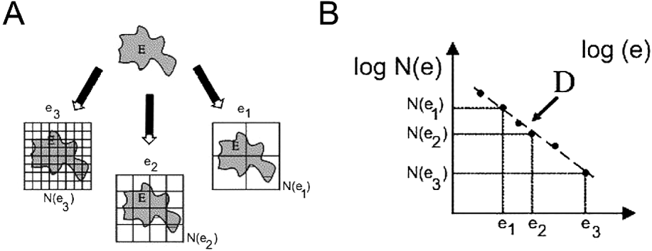
The box-counting method is one of many methods developed for fractal analysis (Soille & Rivet Reference Soille and Rivet1996; Guarino et al., Reference Guarino, Guaccio, Netti and Ambrosio2010). It works by covering a set of data (an image in this case) with ‘boxes’ (squares) and then evaluating how many ‘boxes’ are needed to redescribe the dataset completely in metric space. Repeating this measurement with boxes of decreasing sizes results in a logarithmical function of box size (x-axis) and number of boxes needed to cover the pixels image dataset (y-axis) (Fig. 3). The slope of this function is referred to as the box dimension, which is considered to be a good approximation of the fractal dimension (Soille & Rivet Reference Soille and Rivet1996).
(A) The Box-counting technique applied in a theoretical fractal set (E). (B) Plotting the box number (N (e)) that includes one part of the fractal set (E) at the very least, versus the size of the box (e). D the fractal dimension, is the slope of the straight fitted line. Modified from Rodríguez-Pascua et al. Reference Rodríguez-Pascua, De Vicente, Calvo and Pérez-López2003.
The software we used for our analyses, ‘FrAn’ (for Fractal Analyzer), was created using as a reference a previous program (HarFa), a software that was compiled to perform harmonic and wavelet analysis of digitized images and calculations of their fractal parameters based on the box-counting technique (Harfa 2010). Using this software as an example, we created a new algorithm that also uses the box counting technique, incorporating a new and critical parameter for our aims, the fractal excess (FE) (defined in detail below).
Image data analysis
Using FrAn, we first estimated the fractal dimension of sets images of lichens-colonized and -uncolonized Andean rock surfaces: the images were first trimmed in order to consider unequivocally fully colonized and fully uncolonized selections (Fig. 2). FrAn then transforms these images into grey scale versions, and then to black and white images (Fig. 4). The grey scale to black and white transformation is performed for all possible threshold (T) values (256 in total), where
 $\overline {X} - 1.5\sigma \lt T \lt \overline {X} + 1.5\sigma $, where
 $\overline {X} $ is the mean intensity of all pixels and σ the standard deviation of all pixel intensities. The importance of the thresholding process may be understood if it is considered that the strength of the signal (the brightness and contrast of the image as determined by the intensity value for each pixel) has a direct effect on the amount of information that can be extracted from any particular image (Fig. 5).In practice, this means that every sample image was analysed at least seven times in the range of −1.5σ and 1.5σ. In addition, to every image analysed, a ‘null model’ was created, which corresponded to the same image dataset, but randomized (Fig. 2F).
Image data transformation process. High definition colour images were taken of colonized and uncolonized rocks, and areas of the images where only-colonized and only-uncolonized surfaces were cut and stored. These subsets were then transformed to grey scale and then to black and white images, this last format being the input of fractal analysis.
Threshold importance on subsequent data analysis. As the threshold of black and white images has a direct impact on the amount of information that can reconstruct the original colour image, all threshold values between 0 and 256 were taken into account for subsequent fractal analysis.
Then, the Minkowski–Bouligand dimension (or box dimension) was calculated; ln N(ε)=D box ln (1/ε)+K, where ε is the box length, N is the number of different boxes of size ε and K is an arbitrary constant. This was done for all image analysed and their null counterparts.
After these analyses, computation of the FE was then calculated. The FE is defined as the difference between the fractal spectrum of the sample image fractal spectrum and its null model. Therefore, the incorporation of a null model for each of the samples being analysed guarantees true estimation of the complexity of the analysed images.
Thus, the final output of image data analysis is a curve of the entire spectra of FE values for each threshold situation. As a result, a low FE value indicates a high fractal dimension and correspondingly, a higher complexity of the sample being analysed. In turn, high FE values indicate a low fractal dimension, and thus, a lower complexity of the sample.
All analyses were performed with a Hewlett Packard cluster composed of 62 Intel Titanium II processors and a total of 48 GB of RAM available at the Center for bioinformatics of the Faculty of Biological Sciences of Pontificia Universidad Católica de Chile. Using this processing power, mean analysis time for each image selection was about 20 min. FrAn is available on request.
Results
Figure 6 shows that the FE spectrum curve for all lichen images analysed is unique, and different to the FE spectrum curve for all bare rock surface images. Bare rock samples show higher FE values than lichen FE values, the latter being lower and closer to the x-axis.
FE curves of lichen-colonized and bare rock surfaces. Shaded areas for each curve correspond to the standard error of the means.
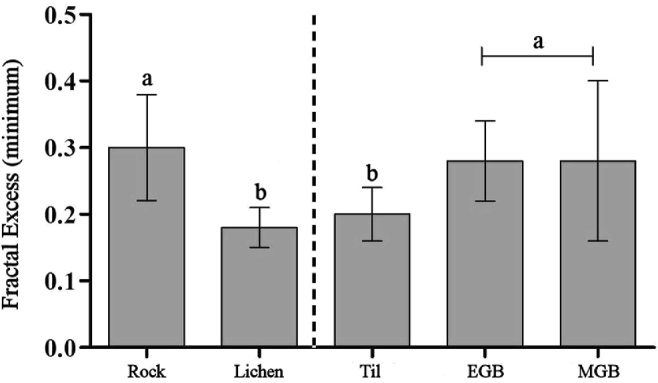
Larger distances between both curves are observed at the positive range of the spectra, although appreciable distances can also be seen at the negative range of the curve. FE minima also reflect these differences, with bare rock surface being 0.26 and Lichen being 0.18 (Fig. 7). At both ends of the FE spectra maxima also follow the same pattern, with lichen maxima being lower than bare rock surface values. This result provides good evidence that biotic processes do have a higher complexity than the environment where they occur.
FE minimum statistical analysis. FE minima of the two models shown were separately analysed by t student test and one-way ANOVA (Tukey's Multiple Comparison post-test), respectively. Means with different letters are significantly different (P<0.05; a>b).
Repeating these analyses in another order of scale shows a similar trend. We processed images of banding vegetation patterns of Tillandsia shrubs growing in the Atacama Desert, comparing them with geological structures of similar appearance, inter-band distance and size in the surrounding area.
As can be seen in Fig. 8, the FE curve profile of vegetation patterns is readily separated from similarly looking geological banding structures. Similar to the results obtained with lichen growth analysis, Tillandsia growing patterns show a curve with lower values than similar abiotic phenomena, thus revealing higher complexity associated with living phenomena. As for FE minima, they also reflect these differences, with geological banding patterns being 0.28 and Tillandsia banding patterns being 0.20 (Fig. 7).
FE curves of different banding processes on Earth and on Mars. Shaded areas for each curve correspond to the standard error.
Interestingly, when similar geological banding patterns found in Meridiani Planum on Mars were analysed, its curve showed a distinctive profile, between those from geological and biological banding patterns on Earth (Fig. 8).
Discussion
As a proof of concept of our approach, we focused on two extreme environments as models, which in addition represent two scales of size (Fig. 1).
First, we analysed lichens growing on rocks at high altitude on the Andes Mountains of Chile. Lichens are important drivers of biogeochemistry and the first lifeforms to colonize barren environments (Cornelissen et al. Reference Cornelissen, Lang, Soudzilovskaia and During2007). Seen from the point of view of an alien civilization, lichens may not be at first recognized as living entities, a hypothetical scenery that emulates a situation in which humans explore an extraterrestrial environment. Hence, we set to determine whether the complexity of lichens could be differentiated from the similarly looking rock background where they grow. By using FrAn we show that indeed, the complexity structures of bare rocks and lichens differ and are readily separable (Fig. 6). Lichen samples have lower FE values than bare rock samples, the former being closer to the x-axis, thus reflecting their higher complexity and entropy. Minima values from both curves reflect this same difference, with the value of lichen minima being much lower than that of bare rock minima (Fig. 7).
In addition, we found that thresholding is useful as a ‘dial’ for extracting the maximum of information for the analysed images. For the case of the lichen model, thresholding in the range of 0 and 1.5 gives better resolution.
Thus, although we have the experimental advantage of ‘knowing’ that lichens are living entities, just by analysing high definition images alone, and with the aid of fractal geometry, we could readily differentiate them as distinct higher entropy entities from its similar abiotic surroundings. By analysing seasonal time series, further spatial and temporal patterns changes in size and/or structure (tridimensional for example) could be incorporated as well.
In order to test our hypothesis on a larger scale, we applied our analysis to banded vegetation patterns of Tillandsia species growing in the Atacama Desert, comparing them with geological banding structures of similar appearance found in the area. Similar to the case of lichen analysis, Tillandsia banding growths also showed lower values than those of similar geological banding patterns, thus confirming their higher complexity. Analogous to the case of the lichen model, curve minima also reflect these differences, with Tillandsia values being lower than geological values (Fig. 8). In this case, thresholding in the range of −1.5 and −0.5 gave a better resolution.
The Tillandsia banding pattern analysis results show that even from afar, life can be distinguished as a distinctive entropy process, distinct from similar abiotic processes.
The curve behaviour of Mars banding patterns with lower FE values than of Earth abiotic banding patterns but higher than biotic banding patterns remains puzzling for now. As the shapes of the curves of Earth and Mars banding patterns are different, but have similar minima, one may speculate if this could this be either reflecting differences in the geological processes that gave rise to both structures or (more interestingly) some limited influence of life processes in the genesis of Mars strata?
It is important to note that our analysis allows estimation of the complexity of datasets being analysed (images in this case), but as in practice the input data for the FrAn software are pixel intensity numerical values, any type of data can be fitted as well (Burlando, Reference Burlando1993). Thus, future examination of extraterrestrial features could be fractally analysed with our method at different informational layers; high-resolution images, thermal images, elemental and isotopic compositions, pH, etc. In this way, complementary fractal data values could be then overlaid in a matrix to calculate a Lifeform Probability Index (LPI) for extant or past life-related phenomena based on their entropy measurements analysis.
Finally, a number of applications may be envisioned for the approach presented here; rovers on distant planets could be ‘taught’ to use the LPI with the aid of artificial intelligence as a way to tag features that human experience intuitively classifies as ‘interesting’. Potential fossil structures could be compared with this method, in order to appraise its true biological origin, both on Earth or elsewhere in the Solar System. Radio signals from potential extraterrestrial civilizations could as well be analysed in search of fractal patterns, as use of fractal mathematics may be considered as a marker of advanced technological development.
Acknowledgements
Armando Azua-Bustos received a Scholarship for graduate studies from CONICYT Chile, and additional financial support from the Millennium Institute for Fundamental and Applied Biology (MIFAB), Chile, from FONDECYT Project no. 1110597 and from the AngelicvM Foundation. Cristian Vega received financial support from the Center for Bioinformatics, Pontificia Universidad Católica de Chile. We also thank Carlos González-Silva, from CENIMA, Iquique, for his help in field sampling, and Cristián Arenas-Fajardo, for his help with statistical analysis of our data.