









1. Introduction
Stellar spectral libraries are fundamental tools in astrophysics, underpinning analyses from stellar atmosphere studies to stellar population synthesis and galactic archaeology. Libraries such as PHOENIX (Husser et al. Reference Husser, Wende-von Berg, Dreizler, Homeier, Reiners, Barman and Hauschildt2013), C3K (Conroy et al. Reference Conroy, Villaume, van Dokkum and Lind2018), OB–PoWR (Hainich et al. Reference Hainich, Ramachandran, Shenar, Sander, Todt, Gruner, Oskinova and Hamann2019), and TMAP (Werner et al. Reference Werner, Deetjen, Dreizler, Nagel, Rauch and Schuh2003) provide high-resolution synthetic spectra across wide ranges of effective temperature (
 $T_{\mathrm{eff}}$
), surface gravity (
 $\log g$
), and metallicity (
 $\log Z$
). These spectra are generated by stellar-atmosphere models that solve the radiative transfer equation together with the atmospheric structure equations using iterative numerical schemes (Hubeny Reference Hubeny2010). Differences in the physical assumptions, numerical methods, and adopted line lists used in these radiative-transfer computations mean that each library spans a particular region of parameter space, with only partial overlaps between them. Consequently, no single library provides complete or continuous coverage, and their grids often contain irregular sampling, discontinuities, and masked wavelength regions arising from incomplete line lists or numerical instabilities. Transitions between libraries can also introduce non-physical changes in spectral features. Any approach aiming to generate continuous spectra must therefore handle missing information, avoid propagating artefacts from unreliable grid points, and remain stable near boundaries where library assumptions differ.
Stellar spectral libraries are used in two closely related but conceptually distinct contexts, both of which impose stringent requirements on the quality and continuity of the underlying spectral grids. In one, they are employed for direct stellar modelling, in which observed stellar spectra are compared with library templates to infer atmospheric parameters such as
 $T_{\mathrm{eff}}$
,
 $\log g$
, and metallicity. In the other case, libraries serve as intermediate building blocks for constructing simple stellar population (SSP) models, in which stellar spectra are combined with isochrones, initial mass functions, and evolutionary prescriptions to generate integrated spectra for composite stellar systems. Widely used frameworks in this latter category include BC03 (Bruzual & Charlot Reference Bruzual and Charlot2003), Flexible Stellar Population Synthesis (FSPS) (Conroy & Gunn Reference Conroy and Gunn2010), Binary Population and Spectral Synthesis (BPASS) (Stanway & Eldridge Reference Stanway and Eldridge2018), and more recently, ProGeny (Robotham & Bellstedt Reference Robotham and Bellstedt2025). While these approaches target different scientific questions, they share a common dependency on the internal consistency, completeness, and smoothness of the underlying stellar spectral grids.
As a consequence of incomplete coverage, heterogeneous assumptions, and irregular sampling in existing libraries, traditional workflows rely on coarse-gridding or interpolation in sparsely populated regions. Interpolation becomes increasingly uncertain when library assumptions change, sampling is irregular, or flux is masked. This limits applications requiring dense coverage in
 $(T_{\mathrm{eff}}, \log g, \log Z)$
, such as stellar population synthesis, Bayesian spectral fitting, or large parameter sweeps in stellar evolution modelling.
On the fitting side, full-spectrum and stellar-population fitting tools such as STARLIGHT (Cid Fernandes et al. Reference Cid Fernandes, Mateus, Sodré, Stasinska and Gomes2005), STECKMAP (Ocvirk et al. Reference Ocvirk, Pichon, Lançon and Thiébaut2006), VESPA (Tojeiro et al. Reference Tojeiro, Heavens, Jimenez and Panter2007), pPXF (Cappellari & Emsellem Reference Cappellari and Emsellem2004; Cappellari Reference Cappellari2017), and Pipe3D (Sánchez et al. Reference Sánchez2016) infer galaxy stellar populations, kinematics, and related physical properties by fitting observed spectra with combinations of stellar or simple stellar population templates. Their performance is therefore tied to the resolution, completeness, and internal consistency of the underlying template grids. On the library-construction side, frameworks such as ProGeny aim to generate smooth spectral templates by interpolating within and across grids, mitigating some of the irregularities inherent in discrete models. However, all interpolation-based approaches face challenges near grid edges, where sampling is sparse or physics changes abruptly, and cannot seamlessly merge heterogeneous libraries into a unified continuous manifold.
Machine learning offers a promising alternative. Data-driven models that learn mappings between physical parameters and spectra provide differentiable, continuous, and high-speed predictions. Early examples include The Cannon (Ness et al. Reference Ness, Hogg, Rix, Ho and Zasowski2015), which introduced a generative framework for label transfer, and The Payne (Ting et al. Reference Ting, Conroy, Rix and Cargile2019), which demonstrated that compact neural networks can emulate Kurucz spectra with high fidelity. Convolutional and deep-learning approaches such as StarNet (Fabbro et al. Reference Fabbro, Venn, O’Briain, Bialek, Kielty, Jahandar and Monty2018) and astroNN (Leung & Bovy Reference Leung and Bovy2019) show strong performance for stellar label inference, while transformer-based models such as GalProTE (Anwar et al. Reference Anwar, Groves, Cortese and Watts2025) illustrate the flexibility of modern architectures for spectral modelling in noisy environments. Despite these advances, existing ML-based spectral emulators are typically trained on single libraries and thus inherit their parameter-space limits, masked-flux artefacts, and internal inconsistencies. They do not attempt forward spectral synthesis across multiple heterogeneous grids, nor do they treat masked flux as uncertain information to be reconstructed.
Machine learning has also been applied to galaxy-scale spectral analysis and redshift inference, including convolutional models (Pasquet et al. Reference Pasquet, Bertin, Treyer, Arnouts and Fouchez2019), autoencoder frameworks for denoising and dimensionality reduction (Portillo et al. Reference Portillo, Parejko, Vergara and Connolly2020), and transformer architectures developed for extracting physical properties from low signal-to-noise spectra. These methods highlight the power of ML for modelling complex spectral behaviour, but they primarily address inverse problems rather than forward stellar spectral synthesis.
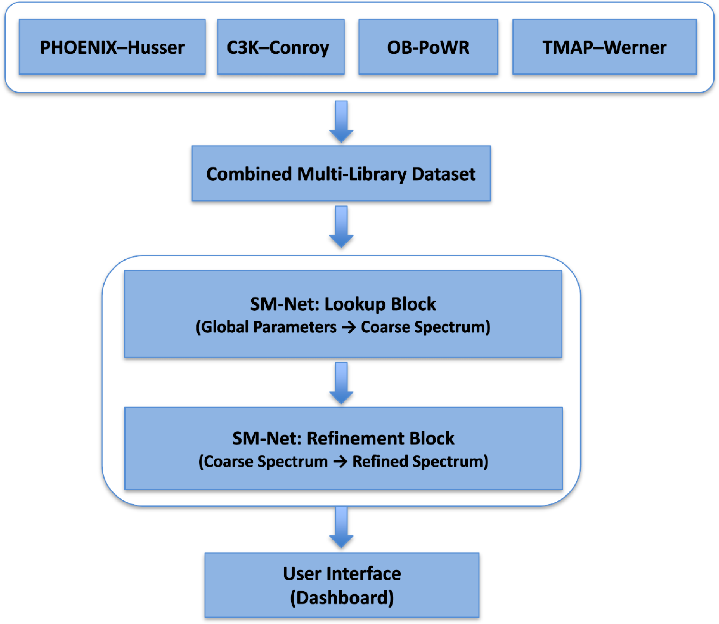
Top-level schematic of the SM-Net model architecture. The four stellar spectral libraries PHOENIX–Husser, C3K–Conroy, OB–PoWR, and TMAP–Werner are first combined into a unified multi-library dataset spanning a broad region of stellar parameter space. SM-Net is then trained on this dataset to generate spectra in two stages: a global parameter-to-coarse-spectrum prediction, followed by a convolutional refinement to produce the final high-fidelity output. The resulting model is accessed through an interactive dashboard that enables real-time spectral generation and exploration.
In this landscape, no existing method learns a unified, continuous spectral manifold spanning multiple high-resolution stellar libraries with overlapping yet heterogeneous parameter ranges. Prior emulators do not address the challenges posed by masked flux regions, library-specific modelling assumptions, or the need for smooth interpolation across inconsistent grid boundaries. Learning across libraries requires reconciling heterogeneous physical assumptions while retaining coherent spectral behaviour. Because each library specialises in different temperature, gravity, and metallicity regimes, a unified model must learn a consistent structure across overlaps and avoid imprinting library-specific artefacts as physical trends. Ensuring smooth, physically plausible predictions in sparsely sampled or rapidly varying regions is essential for applications such as population synthesis, parameter sweeps, and dense template construction.
In this work, we present SM-Net, a machine-learning framework designed to learn a continuous spectral manifold from multiple synthetic stellar libraries, as shown in Figure 1. By combining the grids of PHOENIX–Husser, C3K–Conroy, OB–PoWR, and TMAP–Werner, we construct a composite dataset, with deterministic handling of exact overlaps, that spans a broader region of stellar parameter space than any individual library. The unified grid covers effective temperatures
 $T_{\mathrm{eff}} = 2{\,}000$
–
 $190{\,}000\, \mathrm{K}$
, surface gravities
 $\log g = -1$
–9, and metallicities
 $\log Z = -4$
–1, where we use the standard shorthand
 $\log g \equiv \log_{10}\kern-1.5pt\left(\,g/(\mathrm{cm}\,\mathrm{s}{^{-2}})\right)$
and
 $\log Z \equiv \log_{10}\kern-1.5pt(Z/Z_\odot)$
, with Z denoting the heavy-element mass fraction. SM-Net is trained directly on this combined dataset, treating masked or zero-valued flux samples as unknowns and exploiting local structure in parameter space to infer missing information, over the wavelength range
 $3{\,}000$
–
 $100{\,}000$
Å. The resulting model can generate spectra at arbitrary locations in parameter space within the joint bounds of the combined libraries (i.e. continuous interpolation). We assess the fidelity of these generated spectra not only through flux-level reconstruction metrics but also through synthetic broad-band colours and standard line-strength indices, which test the recovery of integrated and local spectral properties. SM-Net achieves inference speeds exceeding
 $14{\,}000$
spectra per second on a single GPU. To support community use, we also provide a browser-based interactive dashboard enabling real-time exploration of the learned manifold.
Parameter ranges of the stellar spectral libraries used in this work. Surface gravity is reported as
 $\log g \equiv \log_{10}\kern-1.5pt[g/(\mathrm{cm}\,\mathrm{s}{^{-2}})]$
, and metallicity as
 $\log Z \equiv \log_{10}\kern-1.5pt(Z/Z_\odot)$
. N is the number of unique spectra in each source library; SM-Net is trained on the combined dataset and can generate spectra continuously within the sampled parameter bounds, but only predictions within regions supported by the training manifold should be regarded as interpolation.

Table 1. Long description
A table with six rows and seven columns comparing different stellar spectral libraries. The columns are Library, Type, T_eff (K), log g (dex), log Z (dex), λ (Å), and N. The rows are PHOENIX (Husser), C3K (Conroy), OB (PoWR), TMAP (Werner), and SM-Net (combined). Each row lists the type of library, effective temperature range in Kelvin, surface gravity in dex, metallicity in dex, wavelength range in Angstroms, and the number of unique spectra. PHOENIX (Husser) has a base type with a temperature range of 2300-12000 K, surface gravity of 0-6 dex, metallicity of -4-1 dex, wavelength range of 500-55000 Å, and 7559 unique spectra. C3K (Conroy) has a base type with a temperature range of 2000-50000 K, surface gravity of -1-5.5 dex, metallicity of -2.1-0.5 dex, wavelength range of 100-100000 Å, and 8602 unique spectra. OB (PoWR) has a hot type with a temperature range of 15000-56000 K, surface gravity of 2-4.2 dex, wavelength range of 100-100000 Å, and 243 unique spectra. TMAP (Werner) has a white type with a temperature range of 20000-190000 K, surface gravity of 5-9 dex, wavelength range of 3-400000 Å, and 124 unique spectra. SM-Net (combined) is an ML model with a temperature range of 2000-190000 K, surface gravity of 1-9 dex, metallicity of -4-1 dex, wavelength range of 3000-100000 Å.
The remainder of this paper is structured as follows. Section 2 describes the construction of the combined multi-library dataset. Section 3 outlines our preprocessing, normalisation, and augmentation strategy. Section 4 presents the SM-Net architecture and training procedure. Section 5 discusses the cross-library mismatch in detail. Section 6 evaluates performance across the parameter grid. Section 7 presents the web-based interface for SM-Net. Section 8 places SM-Net in the context of existing stellar synthesis workflows, discusses its performance and limitations, and outlines prospects for hybrid physical–machine-learning approaches. Section 9 presents our conclusion and possible future directions.
2. Dataset preparation
In this work, we build directly on the homogenised stellar spectral libraries distributed as part of the ProGeny framework, rather than reprocessing the original model grids from their respective primary sources. These reformatted libraries incorporate several preprocessing steps to improve cross-library consistency and usability, including wavelength resampling onto a common grid, removal of problematic spectra, and physically motivated extrapolation of flux at long wavelengths using black-body extensions where required. Our contribution is therefore not the re-derivation of the underlying stellar atmosphere models, but the unification, augmentation, and modelling of these processed libraries within a single continuous spectral manifold.
The four stellar libraries used in this work, PHOENIX–Husser, C3K–Conroy, OB–PoWR, and TMAP–Werner, are summarised in Table 1. These libraries differ not only in wavelength sampling, parameter coverage, and spectral resolution but also in their underlying atmosphere assumptions. PHOENIX–Husser primarily provides cool-star photospheric spectra based on PHOENIX model atmospheres; C3K–Conroy extends the coverage using a distinct stellar-atmosphere and opacity treatment; OB–PoWR is tailored to hot massive stars and includes non-LTE, wind-sensitive atmospheres; and TMAP–Werner is designed for hot compact stars and white dwarfs. Consequently, spectra with similar or even identical labels are not guaranteed to be physically interchangeable across libraries. This is a central motivation for both the deterministic overlap handling described below and the cross-library mismatch analysis presented in Section 5.
During reformatting by ProGeny, all spectra were resampled onto a common wavelength axis spanning
 $3{\,}000$
–
 $100{\,}000$
Å. Because the PHOENIX–Husser spectra natively extend only to
 $55{\,}000$
Å, the remaining far-infrared region was filled using a physically motivated black-body continuation, providing a smooth thermal continuum without introducing artificial spectral features. A fifth library, PHOENIX–Allard, was also considered but excluded because its spectra exhibited highly irregular behaviour below
 $10{\,}000$
Å and at
 $T_{\mathrm{eff}} \lt 4{\,}000$
K, indicating substantial physical inconsistencies.
In the combined dataset, wavelengths below 3 000 Å were discarded because the four libraries exhibit substantial inconsistencies in this ultraviolet regime, including discontinuities and incompatible flux behaviour. The adopted wavelength grid again follows the ProGeny sampling, which is deliberately non-uniform and feature-aware. This grid allocates dense sampling in wavelength regions containing strong and rapidly varying spectral features, while permitting much coarser sampling in the smooth Rayleigh–Jeans tail at long wavelengths (approaching 100 000 Å), where the spectrum is nearly featureless. A similar philosophy is adopted in the CB19 stellar population models (Plat et al. Reference Plat, Charlot, Bruzual, Feltre, Vidal-García, Morisset, Chevallard and Todt2019), which likewise emphasise high fidelity in feature-rich spectral regions. ProGeny uses the publicly available CB19 stellar spectral grid, which is distributed as a complete model grid rather than described in a dedicated standalone methods paper. The same grid was reused in this work, and therefore provides a practical, well-characterised compromise between spectral fidelity and data volume. After resampling onto this grid, each spectrum contains 11 655 wavelength samples.
Two-dimensional projections of the combined library coverage in
 $\log_{10}\kern-1.5pt(T_{\text{eff}}/\text{K})$
–
 $\log g$
,
 $\log_{10}\kern-1.5pt(T_{\text{eff}}/\text{K})$
–
 $\log Z$
, and
 $\log Z$
–
 $\log g$
parameter space. Each point represents at least one spectrum in the combined dataset after collapsing over the third parameter axis. Colours indicate the contributing library or combination of libraries at each projected location.
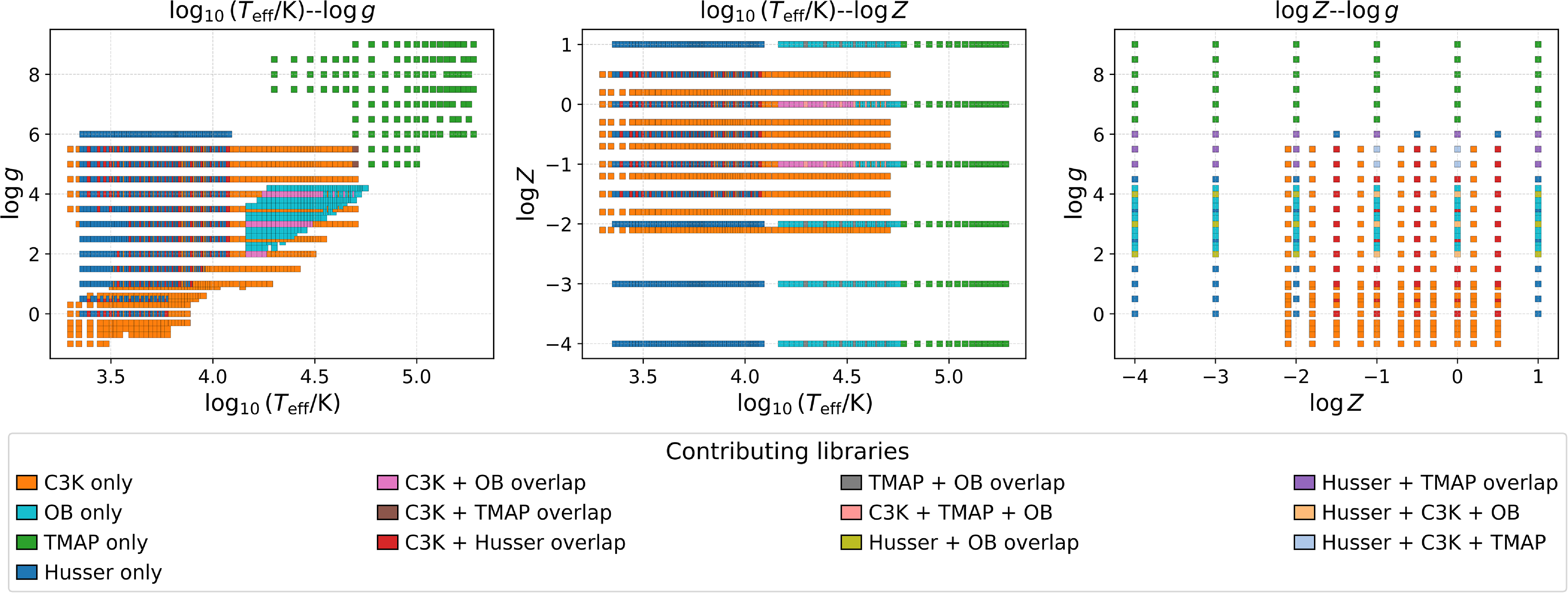
Figure 2. Long description
Panel A: A scatter plot shows the relationship between log10(Teff/K) and log g. The x-axis represents log10(Teff/K) and the y-axis represents log g. Different colors indicate contributions from various libraries or combinations of libraries. Panel B: A scatter plot shows the relationship between log10(Teff/K) and log Z. The x-axis represents log10(Teff/K) and the y-axis represents log Z. Different colors indicate contributions from various libraries or combinations of libraries. Panel C: A scatter plot shows the relationship between log Z and log g. The x-axis represents log Z and the y-axis represents log g. Different colors indicate contributions from various libraries or combinations of libraries.
The total number of spectra in the four libraries is
 $16\,528$
. Since TMAP and OB–PoWR do not include metallicity as a model parameter, they cannot be directly placed into the three-dimensional
 $(T_{\mathrm{eff}}, \log g, \log Z)$
space used by the other libraries. In the grids for these two libraries, metallicity is undefined; all spectra at a given
 $(T_{\mathrm{eff}}, \log g)$
are identical regardless of any value of
 $\log Z$
that might be assigned. To embed TMAP and OB–PoWR into a unified three-parameter space without altering their data structure, each spectrum from these libraries was replicated six times with assigned metallicities
 $\log Z \in \{-4,-3,-2,-1,0,1\}$
. This covers the entire metallicity range on the grid, with a 1 dex interval. This procedure enables dimensional compatibility with the other libraries, allowing the network to learn the intended grid behaviour: in the region of parameter space covered exclusively by TMAP or OB–PoWR, the spectra are invariant under changes in
 $\log Z$
. We emphasise that this invariance is a limitation of the underlying training data rather than a physical property of the stars. While hot stellar spectra are physically affected by metallicity, these effects are absent in the specific source grids used here for this parameter regime.
After replicating the TMAP and OB–PoWR spectra across six assigned metallicity values, the number of spectra from these libraries increased to 744 (
 $124\times6$
) and 1 458 (
 $243\times6$
), respectively, raising the total number of spectra across all four libraries to 18 363. In regions where the
 $(T_{\mathrm{eff}},\log g,\log Z)$
labels coincided exactly, only one spectrum was retained according to the deterministic priority order TMAP
 $\gt $
PHOENIX–Husser
 $\gt $
OB–PoWR
 $\gt $
C3K. Here, exact overlap refers to numerically identical parameter labels after applying the common grid formatting used in this work; no nearest-neighbour or spectral-similarity matching was used during de-duplication. The priority order reflects the specialised parameter regimes of TMAP, PHOENIX–Husser, and OB–PoWR, while C3K provides both complementary overlap coverage and unique coverage at lower effective temperatures. Consequently, all 927 spectra removed during exact-overlap resolution belong to C3K, leaving 17 436 spectra.
A subsequent quality-control step removed 36 OB–PoWR spectra corresponding to all combinations of
 \begin{align*}T_{\mathrm{eff}}\in\{16{\,}000,\,17{\,}000,\,18{\,}000\}\,\mathrm{K},\end{align*}
 \begin{align*}\log g\in\{2.0,\,2.2\},\end{align*}
together with the six assigned metallicity values. These spectra exhibited pronounced discontinuities and abrupt changes in continuum slope that were inconsistent with neighbouring spectra in the grid. Initial training runs that retained these spectra showed that they distorted the locally learned manifold and degraded interpolation for nearby parameter combinations. They were therefore treated as likely numerical or formatting artefacts rather than genuine physical variation. Their removal produced a final combined dataset of 17 400 spectra with unique labels.
These steps of dataset preparation serve three complementary purposes. Replicating the TMAP and OB–PoWR spectra across assigned metallicities embeds their two-parameter grids within the common three-dimensional parameter space without introducing artificial metallicity dependence. Deterministic overlap resolution provides a single, well-defined training target wherever multiple libraries share identical labels, while the quality-control step prevents anomalous spectral shapes from biasing the learned representation. SM-Net is therefore trained to emulate this curated composite dataset rather than to infer a physically unique reconciliation between heterogeneous libraries. In exact-overlap regions, the model learns the retained reference spectrum selected by the imposed priority ordering.
The parameter-space coverage of the combined dataset is summarised through the two-dimensional projections shown in Figure 2. These projections illustrate that the union of PHOENIX–Husser, C3K–Conroy, OB–PoWR, and TMAP–Werner spans a substantially broader and more heterogeneous region of
 $(T_{\mathrm{eff}}, \log g, \log Z)$
than any individual library alone. They also show the irregular shape of the combined grid, the varying sampling density across different regions of parameter space, and the locations of overlap between libraries. Each panel collapses the three-dimensional grid along one parameter axis, showing the coverage and overlap for the remaining two parameters. The
 $T_{\mathrm{eff}}$
axis is shown on a logarithmic scale.
To minimise overlap between the training and validation sets, we constructed the data splits directly in parameter space rather than by random sampling. For each of the three parameters
 $(T_{\mathrm{eff}}, \log g, \log Z)$
, the unique sorted values were assigned to the training and validation sets following a fixed repeating pattern, in which two consecutive values were allocated to the training set and the next two to the validation set. This procedure was applied independently along each parameter axis, such that a spectrum assigned to the training set does not share any of its parameter values with any spectrum in the validation set. The only deliberate exception occurs at the grid boundaries, where the extreme values (the first two and last two grid points along each axis) are included in both splits to ensure stable behaviour near the edges and corners of the parameter space. Here, boundary cases refer specifically to spectra lying at the extremes of the sampled ranges in
 $T_{\mathrm{eff}}$
,
 $\log g$
, or
 $\log Z$
, and are shared solely to anchor interpolation at these limits. Due to the irregular shapes and incomplete overlaps among the individual library grids, only 18 unique parameter triples, corresponding to 18 retained spectra, are shared between the training and validation sets.
Consider three sorted parameter sets from the combined dataset:
 \begin{align*}\begin{aligned}T_{\mathrm{eff}} &= \{t_1,t_2,t_3,t_4,t_5,...\},\\\log g &= \{g_1,g_2,g_3,g_4,g_5,...\},\\\log Z &= \{z_1,z_2,z_3,z_4,z_5,...\}.\end{aligned}\end{align*}
With 2 boundary values (subscript
 $_1$
and
 $_2$
) shared between train and validation, and applying the 2-train and 2-validation pattern independently to each axis, gives
 \begin{align*}T_{\mathrm{eff}}^{\mathrm{train}} &= \{t_1,t_2,t_3,t_4,t_7,...\}, &\quad T_{\mathrm{eff}}^{\mathrm{val}} &= \{t_1,t_2,t_5,t_6,...\},\\\log g^{\mathrm{train}} &= \{g_1,g_2,g_3,g_4,g_7,...\}, &\quad\log g^{\mathrm{val}} &= \{g_1,g_2,g_5,g_6,...\},\\\log Z^{\mathrm{train}} &= \{z_1,z_2,z_3,z_4,z_7,...\}, &\quad\log Z^{\mathrm{val}} &= \{z_1,z_2,z_5,z_6,...\}.\end{align*}
A spectrum belongs to the training set only if all three of its parameter values fall inside the training subsets above; similarly for the validation set. Representative example combinations are shown in Table 2. Any spectrum whose parameters do not fall entirely within either training or validation subsets is assigned to the test set. This demonstrates that the split is defined in parameter space, not by random splits, and that the resulting partitions reflect the true structure of the irregular multi-library grid.
Because the combined grid is formed from four libraries with highly irregular and different parameter coverage, the vast majority of possible
 $(T_{\mathrm{eff}}, \log g, \log Z)$
combinations do not correspond to any real spectrum in any library. Such combinations are discarded and therefore are not allocated to any split.
This splitting scheme forces the model to validate its results on parameter combinations not encountered during training, and hence the validation set provides a strict measure of generalisation for early stopping. Following the removal of the identified outliers in the spectra, the resulting split contains 3 526 training spectra, 2 383 validation spectra, and 11 509 test spectra. Because 18 boundary spectra are deliberately included in both the training and validation sets, these split counts sum to 17 418 entries but correspond to 17 400 unique retained spectra. Although this produces a relatively large test split and smaller training and validation splits, which is unconventional in machine learning, the resulting parameter distributions remain well spread across the grid, ensuring adequate training coverage and a fair evaluation of interpolation at unseen parameter combinations.
Illustrative assignment of spectra to train/validation/test sets based on the 2–2 parameter split pattern. Ticks indicate membership; boundary cases appear in both the training and validation sets.
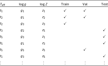
Table 2. Long description
A table with 10 rows and 5 columns. The columns are labeled T eff, log g, log Z, Train, Val, and Test. The rows are labeled with different combinations of T eff, log g, and log Z values. Ticks indicate membership in the Train, Val, or Test sets. Boundary cases appear in both the training and validation sets. Row 1: T eff t1, log g g1, log Z z1, Train tick, Val tick. Row 2: T eff t2, log g g1, log Z z2, Train tick, Val tick. Row 3: T eff t2, log g g3, log Z z3, Train tick. Row 4: T eff t3, log g g2, log Z z5, Test tick. Row 5: T eff t5, log g g3, log Z z1, Val tick. Row 6: T eff t5, log g g1, log Z z3, Test tick. Row 7: T eff t5, log g g5, log Z z5, Val tick. Row 8: T eff t1, log g g3, log Z z5, Test tick. Row 9: T eff t, log g g, log Z z. Row 10: T eff t, log g g, log Z z.
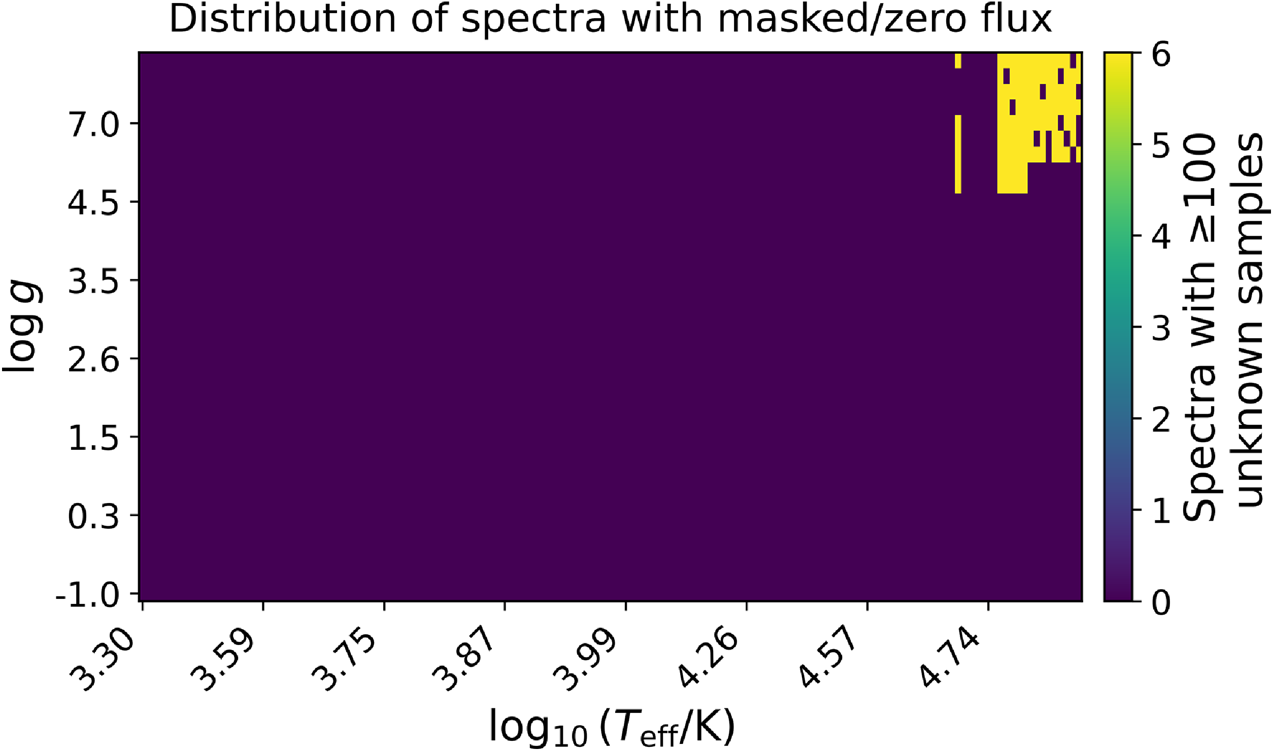
Missing or invalid flux values were identified through NaN and zero-value detection, with zero-valued regions treated as masked intervals rather than physical flux. A bounded zero-run analysis was applied to detect internal masked regions without trimming spectra, preserving as much surrounding information as possible. Figure 3 shows the distribution of unknown flux values in the combined dataset, where more than 100 flux values per spectrum were missing. For the wavelength range of
 $3\,000$
–
 $100\,000$
Å, all of the spectra with missing flux regions belong to the TMAP library.
Distribution of zero/unknown flux values across the dataset of combined grids. Counts are aggregated over
 $\log Z$
values.
For model training and evaluation, flux values in the combined dataset were mapped to the interval [0, 1] using a log1p-based scaling. This transformation compresses the large dynamic range of stellar spectra while remaining strictly monotonic in the original flux. In practice, we adopt a numerically stable implementation in which zero-valued flux elements remain exactly zero, and the logarithmic scale is set adaptively using a small percentile of the positive flux distribution to avoid sensitivity to extreme outliers. The resulting spectra are normalised using a dataset-wide maximum flux, ensuring consistent scaling across libraries with differing absolute normalisations. Although this nonlinear transformation alters linear flux ratios, it preserves the relative ordering of spectral features and stabilises optimisation without introducing spurious structure into masked or low-flux regions.
3. Spectral similarity and augmentation strategy
A key challenge in training an ML model is constructing a balanced training dataset. Unlike typical classification or regression problems where class imbalance arises from having many examples of some classes and few of others, this combined dataset contains a single spectrum for each unique triplet/class of
 $(T_{\mathrm{eff}}, \log g, \log Z)$
. In this case, the imbalance instead arises from the underlying structure of the stellar parameter grid. Certain parts of the grid are densely sampled and contain spectra whose shapes change only gradually across neighbouring points, resulting in many regions with nearly identical spectra. In contrast, other areas of the grid exhibit sharp spectral transitions but contain relatively few grid points. This leads to a biased distribution of spectral shapes, with some spectral morphologies appearing abundantly while others are represented by only a handful of examples.
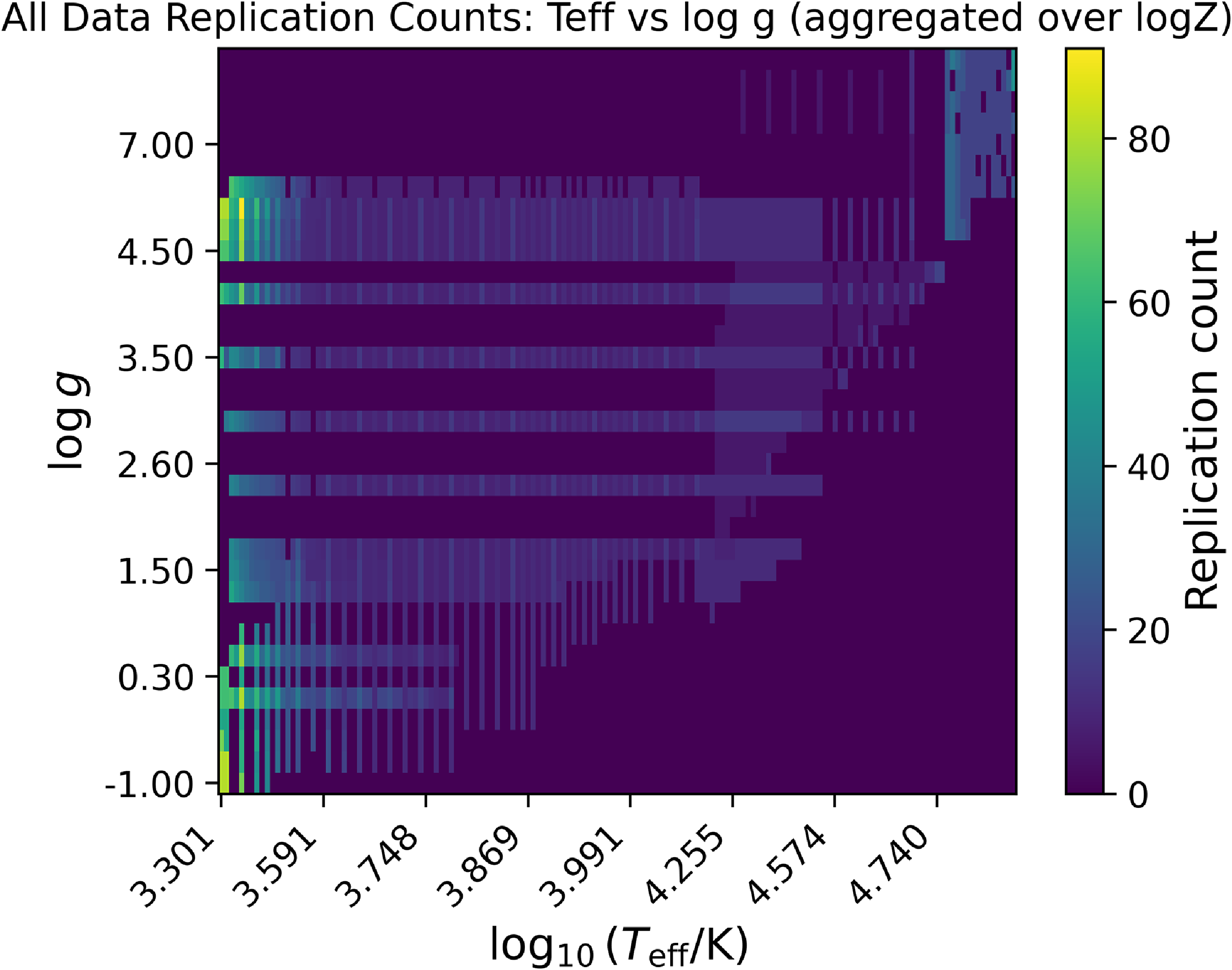
To correct for this imbalance, we computed pairwise cosine similarity across the combined dataset, supplemented by a masked L1 distance that excludes wavelength intervals with zero flux. These measures quantify the relative uniqueness of each spectrum while emphasising meaningful differences in spectral morphology. Spectra identified as more distinctive were assigned higher repeat counts, up to a maximum of 10, whereas spectra that were highly similar to other grid members received no repetition. As a result, about 20% of the spectra in the combined dataset are repeated more than once, whereas the remaining 80% appear only once. The repeat plan does not generate new spectra or new parameter combinations; it only changes how frequently existing spectra are represented. After applying this plan, the training, validation, and test splits contain 5 742, 3 836, and 11 509 rows, respectively, as shown in Table 3. Figure 4 shows the resulting replication counts in the
 $T_{\mathrm{eff}}$
–
 $\log g$
grid after aggregation over
 $\log Z$
. Many of the spectra assigned larger repeat counts lie in the low-temperature regime, where spectral morphology changes rapidly and distinctive molecular features are common.
Number of spectra in each dataset split before and after augmentation based on spectral uniqueness. The test set was not augmented for model evaluation.
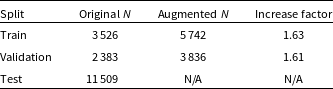
Table 3. Long description
The table has three rows and four columns. The columns are labeled Split, Original N, Augmented N, and Increase factor. The rows are labeled Train, Validation, and Test. Row 1: Train, Original N 3 526, Augmented N 5 742, Increase factor 1.63. Row 2: Validation, Original N 2 383, Augmented N 3 836, Increase factor 1.61. Row 3: Test, Original N 11 509, Augmented N N/A, Increase factor N/A.
The validation set was also augmented because early stopping relies on its loss as a proxy for generalisation and must therefore remain sensitive to rare and difficult spectral morphologies. Weighting distinctive validation spectra more strongly prevents the early-stopping criterion from being dominated by the most common spectral shapes. The test set was not replicated for model evaluation, so that each test spectrum contributes once to the reported performance statistics. Overall, the augmentation increases the influence of rare spectral shapes during training and validation without altering the composition of the test evaluation.
4. Model architecture and training
SM-Net consists of two main blocks: a global parameter–to–spectrum predictor (Lookup Block) and a convolutional refinement module (Refinement Block), as shown in Figure 5. Together, these blocks map the three input stellar parameters
 \begin{equation*}\mathbf{x} = [T_{\mathrm{eff}} \quad \log g \quad \log Z],\end{equation*}
to a full-resolution spectrum of length
 $L = 11\,655$
. The Lookup Block provides a smooth coarse estimate, while the Refinement Block adds wavelength-dependent corrections to produce the final high-fidelity output.
The replication counts for the entire dataset based on spectral dissimilarity, aggregated over
 $\log Z$
.
Block-level architecture of SM-Net, showing the two-stage mapping from stellar parameters to a high-resolution synthetic spectrum. The Lookup Block takes the input parameters (effective temperature, surface gravity, and metallicity) and produces a coarse, low-frequency spectral estimate through a sequence of embedding, fully connected, and projection layers. This coarse spectrum, together with the physical parameters and positional encodings, is passed to the Refinement Block, where convolutional feature extractors and residual convolutional blocks learn wavelength-dependent corrections. The refinement output is added to the coarse spectrum to produce the final high-resolution stellar spectrum.
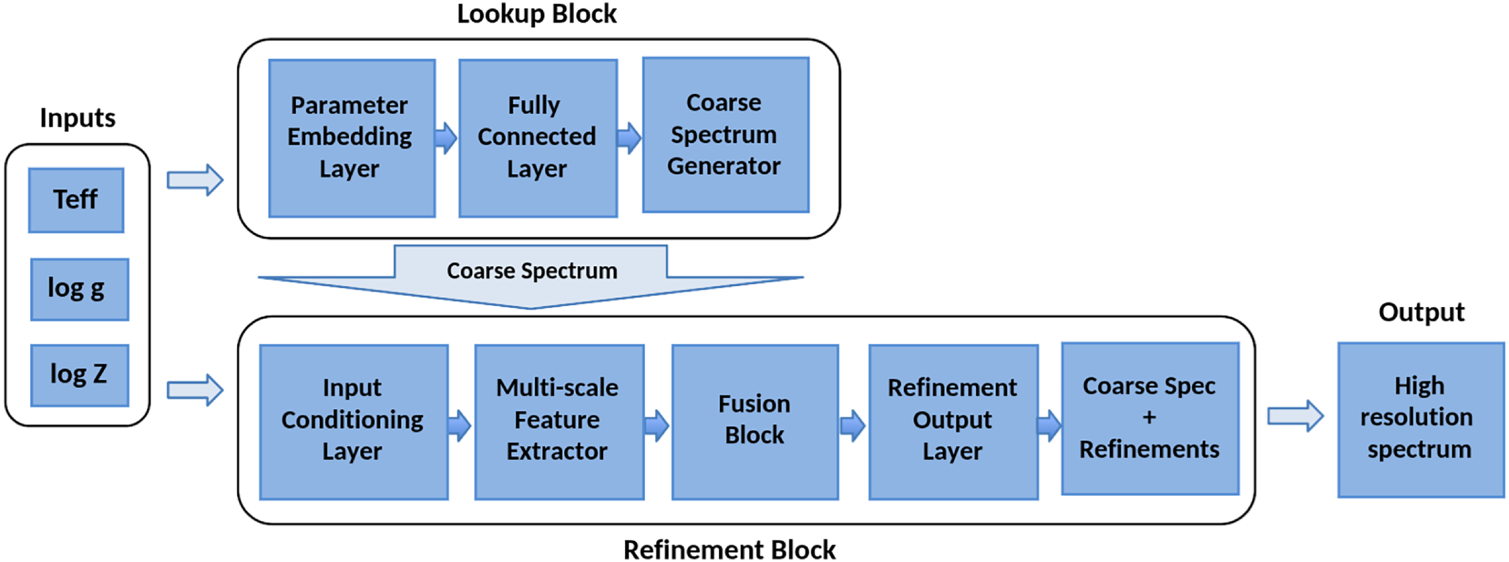
Figure 5. Long description
A diagram of the block-level architecture of SM-Net, showing the two-stage mapping from stellar parameters to a high-resolution synthetic spectrum. The diagram includes two main blocks: the Lookup Block and the Refinement Block. The Lookup Block takes input parameters (effective temperature, surface gravity, and metallicity) and produces a coarse, low-frequency spectral estimate through a sequence of embedding, fully connected, and projection layers. The Refinement Block takes the coarse spectrum, along with the physical parameters and positional encodings, and uses convolutional feature extractors and residual convolutional blocks to learn wavelength-dependent corrections. The refinement output is added to the coarse spectrum to produce the final high-resolution stellar spectrum.
4.1. Lookup block: Global parameter-to-spectrum mapping
The first stage of SM-Net is the Lookup Block, which transforms the three-dimensional input parameters into a coarse, low-frequency spectral prediction. In terms of the architecture in Figure 5, this stage consists of:
-
• a Parameter Embedding Layer that expands the physical inputs into a higher-dimensional representation,
-
• three Fully Connected Layers, with dimensions
 $3 \rightarrow 4\,096 \rightarrow 16\,384 \rightarrow 11\,655$
, implemented using residual MLP blocks,
-
• a Coarse Spectrum Generator that produces an initial spectral estimate.

The embedded parameters pass through two residual fully connected layers:
 \begin{align}\mathbf{h}_1 &= f_1(\mathbf{x}) + P_1(\mathbf{x}), \end{align}
 \begin{align}\mathbf{h}_2 &= f_2(\mathbf{h}_1) + P_2(\mathbf{x}), \end{align}
where
 $f_1$
and
 $f_2$
are residual MLP blocks, and
 $P_1, P_2$
are linear skip projections that forward the physical parameters directly to deeper layers.
The Coarse Spectrum Generator produces the initial coarse spectrum:
 \begin{equation}\mathbf{s}_{\mathrm{coarse}} = W_3 \mathbf{h}_2 + P_3(\mathbf{x}),\end{equation}
where
 $W_3$
is a learned linear operator and
 $P_3$
is the final linear layer of this block, mapping output to the spectral dimension.
A learnable per-wavelength baseline vector
 $\mathbf{b} \in \mathbb{R}^{L}$
is initialised to the median flux of the training data. This baseline acts as a stabilising prior on the predicted spectrum. It is applied using a Softplus transformation,
 \begin{equation}\mathbf{s}_0 = \mathrm{Softplus}_\beta\!\left( \mathbf{s}_{\mathrm{coarse}} + \mathbf{b} \right)\!,\end{equation}
which guarantees non-negative output fluxes. The parameter
 $\beta$
controls the sharpness of the Softplus activation.
4.2. Refinement block: Residual spectral refinement
The second stage of SM-Net is the Refinement Block, which applies a series of convolutional operations to refine the coarse prediction with detailed wavelength-dependent corrections. Architecturally, this block consists of:
-
• an Input Conditioning Layer that integrates the learned conditioning vector, a fixed three-channel positional encoding, and the coarse spectrum;
-
• a Multi-scale Feature Extractor consisting of three parallel convolutional branches with kernel sizes of 7, 15, and 23;
-
• a Fusion Block that aggregates features from the parallel branches;
-
• a Refinement Output Layer that predicts the additive spectral correction.
The stellar parameters are first expanded along the wavelength axis by a learned linear map:
 \begin{equation} \mathbf{c} = Q\,\mathbf{x} + \mathbf{b}, \end{equation}
where
-
•
$\mathbf{x} \in \mathbb{R}^{D}$
is the input parameter vector (where
$D = 3$
); -
•
$Q \in \mathbb{R}^{L \times D}$
is the learned weight matrix projecting parameters onto the spectral axis; -
•
$\mathbf{b} \in \mathbb{R}^{L}$
is the bias vector; -
•
$\mathbf{c} \in \mathbb{R}^{L}$
is the resulting conditioning vector.


Here L denotes the length of the spectrum.
To provide the refinement module with an explicit notion of spectral position, we generate a fixed three-channel positional encoding
 $\mathbf{P} \in \mathbb{R}^{3 \times L}$
. For a normalised wavelength index
 $t_i \in [0, 1]$
at bin i, the encoding channels are defined as:
 \begin{equation} \mathbf{P}_i = \begin{bmatrix} t_i \\ \sin\! (2\pi t_i) \\ \cos\!(2\pi t_i) \end{bmatrix}. \end{equation}
The Input Conditioning Layer concatenates the coarse spectrum
 $\mathbf{s}_0$
, the conditioning vector
 $\mathbf{c}$
, and the three-channel positional encoding
 $\mathbf{P}$
along the channel dimension:
 \begin{equation} \mathbf{X} = \begin{bmatrix} \mathbf{s}_0^{\top} \\ \mathbf{c}^{\top} \\ \mathbf{P} \end{bmatrix} \in \mathbb{R}^{5 \times L}. \end{equation}
Thus,
 $\mathbf{X}$
contains one channel from
 $\mathbf{s}_0$
, one channel from
 $\mathbf{c}$
, and three channels from
 $\mathbf{P}$
.
The Multi-scale Feature Extractor processes
 $\mathbf{X}$
through three parallel branches to capture features at different scales. For each kernel size
 $k \in \{7, 15, 23\}$
, the output
 $\mathbf{u}_k$
is computed as:
 \begin{equation} \mathbf{u}_k = \mathcal{D}\left( \phi\left( \mathrm{Conv}_k\left( \mathrm{pad}_k(\mathbf{X}) \right) \right) \right)\!, \end{equation}
where
 $\mathrm{pad}_k(\!\cdot\!)$
denotes replicate padding,
 $\phi$
is the GELU activation, and
 $\mathcal{D}$
denotes Dropout. The feature maps from the parallel branches, each corresponding to a different kernel size k, are concatenated along the channel dimension to form a composite multi-scale feature map
 $\mathbf{U}$
. This aggregation allows the network to process local spectral lines and broader continuum features simultaneously. The composite map is processed by a Fusion Block:
 \begin{equation} \mathbf{h} = \mathcal{D}\left( \phi\left( \mathrm{Conv}_{\mathrm{fuse}}(\mathbf{U}) \right) \right)\!. \end{equation}
Here,
 $\mathrm{Conv}_{\mathrm{fuse}}$
represents a convolutional layer designed to mix information across the spectral channels. Finally, the Refinement Output Layer projects these fused features down to a single dimension to produce the scalar spectral correction
 $\Delta\mathbf{s}$
:
 \begin{equation} \Delta\mathbf{s} = \mathrm{Conv}_{\mathrm{out}}(\mathbf{h}). \end{equation}
The final high-resolution spectrum is obtained via a residual connection, where the learned correction is added to the initial coarse estimate:
 \begin{equation} \mathbf{s}_{\mathrm{final}} = \mathbf{s}_0 + \Delta\mathbf{s}. \end{equation}
4.3. Loss function and treatment of masked flux
To handle masked or zero-valued flux (originating from incomplete line lists or numerical issues), SM-Net uses a weighted mean-squared error (MSE) loss:
 \begin{equation}\mathcal{L} =\frac{1}{BL}\sum_{i=1}^{B}\sum_{\lambda=1}^{L}w_\lambda\, m_{i,\lambda}\,\left( s_{i,\lambda} - t_{i,\lambda} \right)^2,\end{equation}
where:
-
• B is the batch size,
-
•
$w_\lambda$
is a per-wavelength weight, -
•
$t_{i,\lambda}$
and
$s_{i,\lambda}$
are the target and predicted fluxes, -
•
$m_{i,\lambda}$
is a binary mask:
\begin{align*}m_{i,\lambda} =\begin{cases}0, & t_{i,\lambda} = 0 \ (\text{masked or uncertain flux}),\\1, & \text{otherwise}.\end{cases}\end{align*}


Masked flux values therefore exert no penalty, allowing the model to reconstruct missing structure by relying on neighbouring wavelengths and on the broader learned relationships encoded in the network.
4.4. Training strategy
The SM-Net model was first trained, evaluated and refined separately on each of the four core libraries. This initial evaluation phase not only guided model optimisation but also revealed regions within individual libraries where the spectra exhibited internal inconsistencies. Below 3 000 Å individual-library training and direct cross-library inspection revealed abrupt continuum offsets, discontinuous slopes, and mutually inconsistent flux amplitudes at neighbouring or matched parameter locations; this region was therefore excluded rather than treated as a physically coherent common domain.
Model training used the Adam optimiser for Learning Rate (LR) scheduling, with an initial LR of
 $4\times 10^{-4}$
and an initial batch size of
 $1\,024$
. Whenever the validation loss failed to improve for ten consecutive epochs, both the LR and batch size were reduced by a factor of
 $0.8$
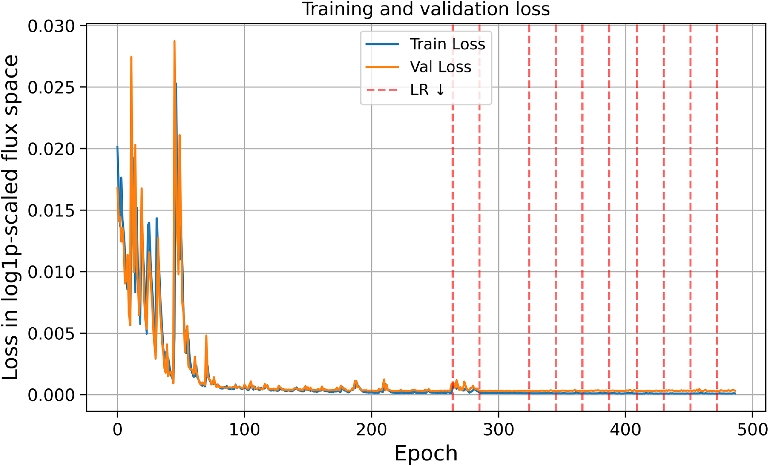
, with a minimum batch size capped at 128. Early stopping was triggered after 50 epochs without improvement. This decay schedule in LR and reduction in training batch size, shown as red dotted lines in Figure 6, served two complementary roles. Large batches in early epochs stabilised the optimisation landscape and enabled the network to learn broad, global spectral trends, whereas progressively smaller batches introduced beneficial gradient noise that helped the optimiser escape shallow minima and focus on fine-grained spectral structure. Reducing the LR in tandem ensured that later stages of training refined subtle features without overshooting, which is essential for high-resolution spectra, where neighbouring wavelengths differ only marginally in flux. Empirically, this coupled decay of batch size and LR yielded smoother convergence than adjusting either hyper-parameter alone.
Training and validation losses throughout the training process. Red lines indicate the epochs at which the learning rate and the batch size were reduced, both by a factor of 0.8.
We enabled automatic mixed-precision with CUDA, using bfloat16 throughout training without gradient scaling. This reduced memory pressure during convolutional refinement without degrading accuracy. Training required a peak GPU memory of 21 GB, whereas inference with a batch size of 256 spectra requires about
 $4.5$
GB of GPU memory. The model achieves rates of approximately
 $14\,000$
spectra per second on a single NVIDIA RTX 4090 GPU. For maximum throughput and full GPU utilisation, the number of inferred spectra should exceed a few thousand. For small inference jobs, the GPU is under-utilised, kernel-launch overheads dominate, and the resulting throughput is noticeably lower than the peak rate.
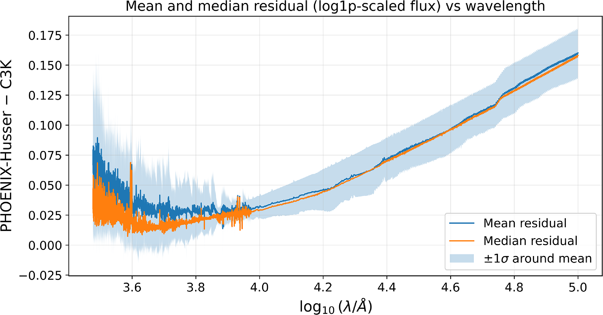
Mean and median residuals between matched PHOENIX–Husser and C3K spectra as a function of
 $\log_{10}\kern-1.5pt(\lambda/$
Å). Residuals are defined as Husser
 $-$
C3K and are computed in the log1p-scaled flux representation across 783 matched
 $(T_{\text{eff}}, \log g, \log Z)$
grid points. The shaded region indicates the
 $\pm 1\sigma$
dispersion of the residuals.
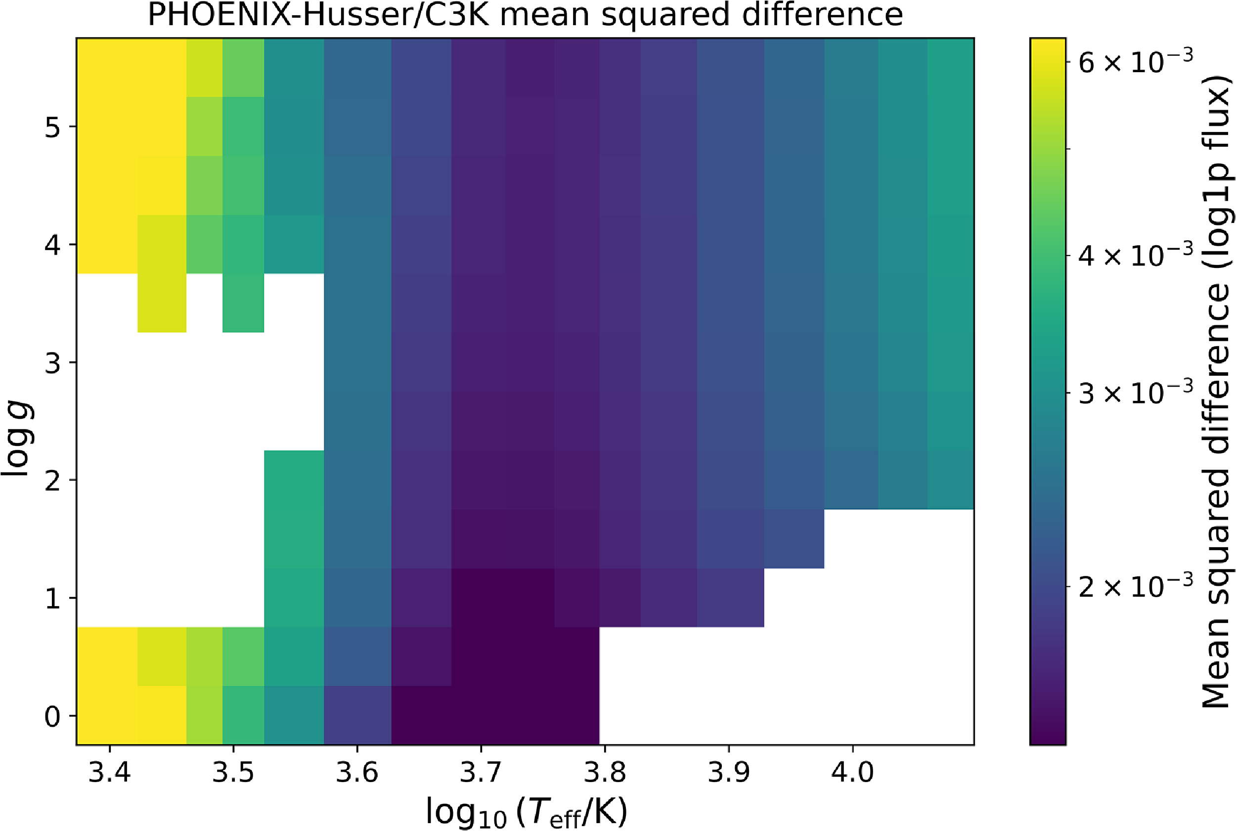
Mean squared difference between matched PHOENIX–Husser and C3K spectra across the common parameter grid, shown in the
 $\log_{10}\kern-1.5pt(T_{\text{eff}}/\text{K})$
–
 $\log g$
plane. The vertical axis shows
 $\log g$
. Values are computed in the log1p-scaled flux representation and averaged over
 $\log Z$
.
5. Cross-library physics mismatches
The mismatch in the underlying physics between different stellar libraries directly affects the accuracy that SM-Net can achieve. This mismatch between some libraries is significant. Figure 7 shows the mean and median residuals when comparing the 783 spectra with the exact same
 $T_{\mathrm{eff}}$
,
 $\log g$
, and
 $\log Z$
labels between the PHOENIX–Husser and C3K libraries, highlighting the mismatch in the physics between the two libraries. Figure 8 shows the mean squared difference between matched PHOENIX–Husser and C3K spectra in the
 $\log_{10}\kern-1.5pt(T_{\mathrm{eff}}/\mathrm{K})$
–
 $\log g$
plane, averaged over
 $\log Z$
. The largest differences occur at lower temperatures, as indicated by the bright yellow regions.
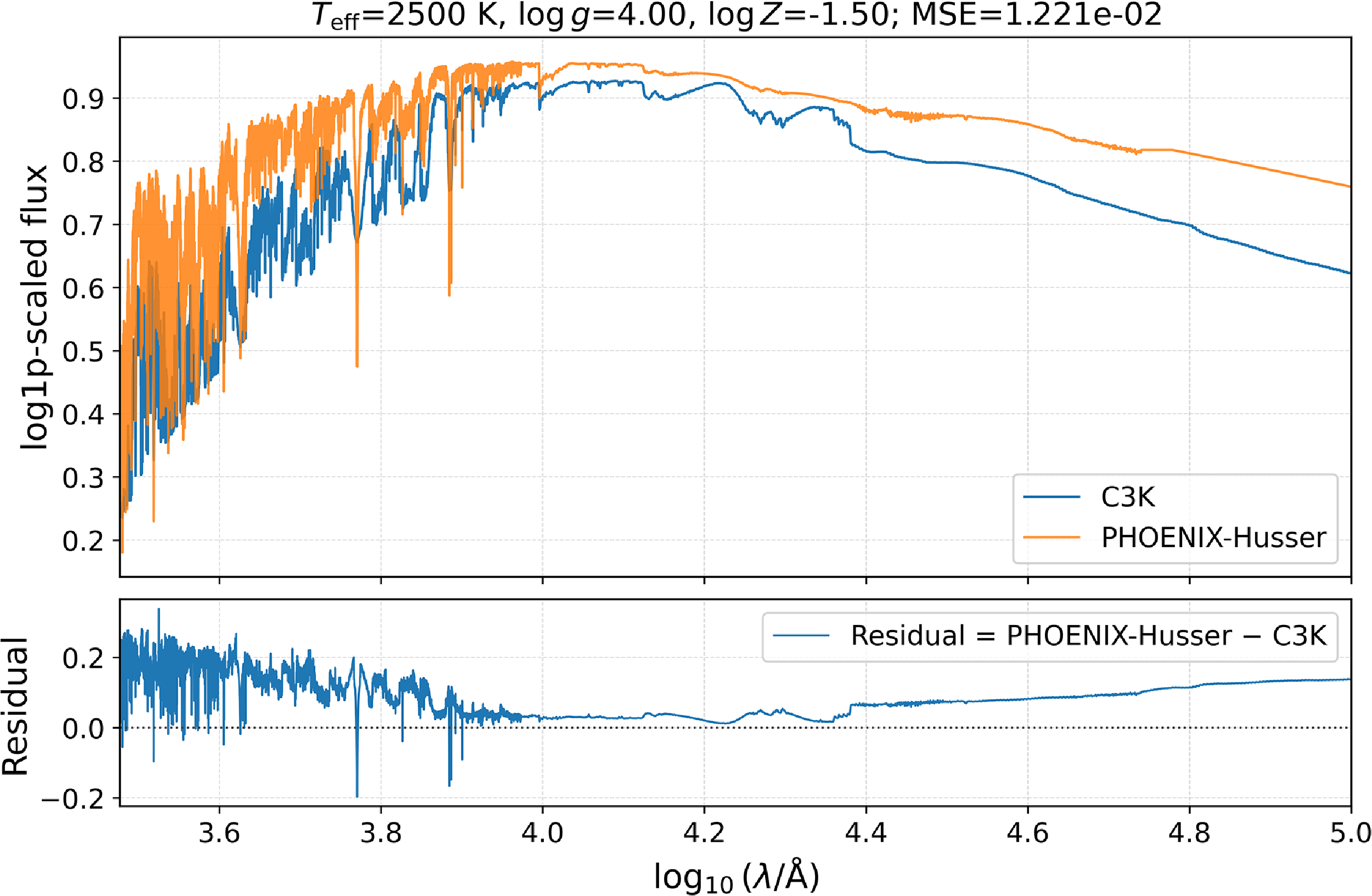
Figure 9 illustrates the mismatch using two original spectra with identical parameters (
 $T_{\mathrm{eff}}=2\,500$
K,
 $\log g=4.0$
,
 $\log Z=-1.5$
) drawn from the two libraries, alongside their residual spectrum. At shorter wavelengths, the flux difference between the spectra from two libraries exceeds 20% and remains as high as
 $\sim$
15% at the longest wavelengths, highlighting a substantial underlying physical mismatch. The consequences of these cross-library mismatches become evident in the reconstruction-error distributions presented in the next section, particularly near overlap boundaries and in sparsely sampled regimes.
Comparison between C3K and PHOENIX–Husser spectra for
 $T_{\text{eff}} = 2\,500\,\text{K}$
,
 $\log g = 4.0$
, and
 $\log Z = -1.5$
. The upper panel shows the two matched library spectra, while the lower panel shows the residual, defined as Husser
 $-$
C3K. The residual highlights the underlying differences in the physics between the two libraries.
6. Evaluation and performance
In this section, we evaluate the quantitative and qualitative reconstruction performance of SM-Net across the training, validation, and test sets. All spectra are represented in the log1p-scaled flux space as described in Section 2, and this transformation is not inverted at any stage of training or evaluation, with the exception of Section 6.2. Consequently, all residuals and mean squared error (MSE) values reported here are computed directly in the log1p-scaled space and should not be interpreted as errors in linear flux units.
First, we analyse the reconstruction accuracy as a function of the three physical parameters
 $(T_{\mathrm{eff}}, \log g, \log Z)$
across the training, validation, and test splits. As discussed in Section 2, spectra from the TMAP and OB–PoWR libraries were replicated across discrete
 $\log Z$
values to enable embedding within the joint parameter space. In metallicity bins populated exclusively by these libraries, the spectra are therefore invariant by construction with respect to
 $\log Z$
and do not probe metallicity-dependent spectral sensitivity. This limitation should be borne in mind when interpreting the error distributions shown in Figures 10–12.
Distribution of MSE prediction errors across
 $\log_{10}\kern-1.5pt(T_{\text{eff}}/\text{K})$
. High MSE occurs predominantly at low temperatures, with consistent trends across splits, indicating robust generalisation.
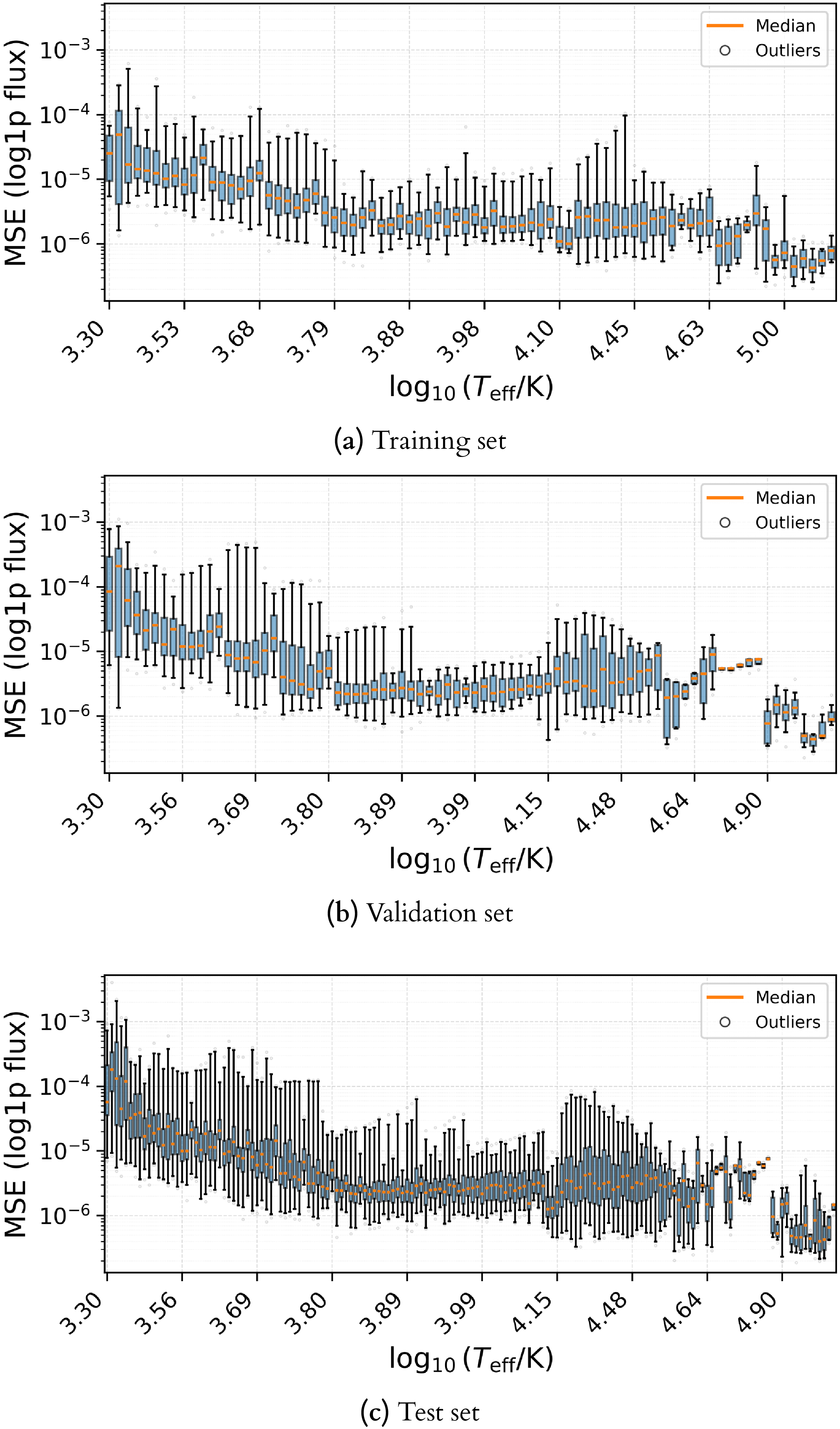
Figure 10. Long description
Panel A: A box plot displays the distribution of MSE (log1p flux) prediction errors across different temperature ranges (log10(Teff/K)) for the training set. The x-axis represents the logarithm of effective temperature in Kelvin, ranging from approximately 3.30 to 5.00. The y-axis represents the MSE in logarithmic scale. The plot includes median values and outliers. Panel B: A box plot shows the distribution of MSE (log1p flux) prediction errors across different temperature ranges (log10(Teff/K)) for the validation set. The x-axis represents the logarithm of effective temperature in Kelvin, ranging from approximately 3.30 to 5.00. The y-axis represents the MSE in logarithmic scale. The plot includes median values and outliers. Panel C: A box plot illustrates the distribution of MSE (log1p flux) prediction errors across different temperature ranges (log10(Teff/K)) for the test set. The x-axis represents the logarithm of effective temperature in Kelvin, ranging from approximately 3.30 to 5.00. The y-axis represents the MSE in logarithmic scale. The plot includes median values and outliers.
Distribution of MSE across
 $\log g$
. Elevated errors occur in validation and test sets near the lower boundary of OB–PoWR (around 2.20), indicating inconsistencies in the underlying physics of the three overlapping libraries in this region.

Distribution of MSE across
 $\log Z$
. Errors are broadly uniform, with particularly low mean and median MSEs at
 $\log Z=-4$
and
 $-3$
, which originate from regions governed by a single library and therefore contain no cross-library inconsistencies.

Figure 12. Long description
Panel A: A box plot showing the distribution of MSE (log1p flux) across different log Z values for the training set. The x-axis represents log Z values ranging from -4.00 to 1.00, and the y-axis represents MSE (log1p flux) ranging from 10^-6 to 10^-3. The plot includes median lines and outliers. Panel B: A box plot showing the distribution of MSE (log1p flux) across different log Z values for the validation set. The x-axis represents log Z values ranging from -4.00 to 1.00, and the y-axis represents MSE (log1p flux) ranging from 10^-6 to 10^-3. The plot includes median lines and outliers. Panel C: A box plot showing the distribution of MSE (log1p flux) across different log Z values for the test set. The x-axis represents log Z values ranging from -4.00 to 1.00, and the y-axis represents MSE (log1p flux) ranging from 10^-6 to 10^-3. The plot includes median lines and outliers.
Table 4 summarises the reconstruction performance across the three dataset splits. The mean per-spectrum MSE values are
 $1.03\times10^{-5}$
for the training set,
 $2.50\times10^{-5}$
for the validation set, and
 $1.97\times10^{-5}$
for the test set. These values correspond to root-mean-square deviations of
 $0.32\%$
,
 $0.50\%$
, and
 $0.44\%$
, respectively, in the normalised log1p-scaled flux representation used for training and evaluation. The median MSE values range from
 $3.42\times10^{-6}$
to
 $4.64\times10^{-6}$
, corresponding to RMS deviations of approximately
 $0.18$
–
 $0.22\%$
. This indicates that the majority of spectra are reconstructed with substantially better than
 $0.5\%$
RMS accuracy in the transformed representation.
Summary of SM-Net reconstruction quality across the combined multi-library dataset. For each split, N is the number of unique spectra in the original, unaugmented split, mean MSE is the mean per-spectrum mean squared error, and
 $\text{RMS}_{\text{flux}}$
is the corresponding root-mean-square flux deviation. Percentiles and minimum/maximum values are computed over the per-spectrum MSE distribution.

Table 4. Long description
A table with four columns and three rows summarizing SM-Net reconstruction quality across different dataset splits. The columns are labeled Split, N, Mean MSE, RMS_flux (%), Median MSE, 10th perc. MSE, 90th perc. MSE, Min MSE, and Max MSE. Row 1: Split, Train; N, 3526; Mean MSE, 1.03 x 10^-5; RMS_flux (%), 0.32; Median MSE, 3.42 x 10^-6; 10th perc. MSE, 9.56 x 10^-7; 90th perc. MSE, 1.95 x 10^-5; Min MSE, 2.05 x 10^-7; Max MSE, 6.17 x 10^-4. Row 2: Split, Validation; N, 2383; Mean MSE, 2.50 x 10^-5; RMS_flux (%), 0.50; Median MSE, 4.64 x 10^-6; 10th perc. MSE, 1.32 x 10^-6; 90th perc. MSE, 4.08 x 10^-5; Min MSE, 2.27 x 10^-7; Max MSE, 1.12 x 10^-3. Row 3: Split, Test; N, 11509; Mean MSE, 1.97 x 10^-5; RMS_flux (%), 0.44; Median MSE, 4.26 x 10^-6; 10th perc. MSE, 1.28 x 10^-6; 90th perc. MSE, 3.16 x 10^-5; Min MSE, 1.88 x 10^-7; Max MSE, 4.02 x 10^-3.
The 10th-percentile MSE values range from
 $9.56\times10^{-7}$
to
 $1.32\times10^{-6}$
, corresponding to RMS deviations of approximately
 $0.10$
–
 $0.11\%$
. These values characterise the best reconstructed portion of each split, for which SM-Net achieves particularly close agreement with the reference spectra. The 90th-percentile MSE values range from
 $1.95\times10^{-5}$
to
 $4.08\times10^{-5}$
, corresponding to RMS deviations of approximately
 $0.44$
–
 $0.64\%$
. Thus, 90% of the spectra in each split have reconstruction errors below approximately
 $0.7\%$
RMS in the transformed flux representation.
The minimum MSE values range from
 $1.88\times10^{-7}$
to
 $2.27\times10^{-7}$
, corresponding to RMS deviations below
 $0.05\%$
. These cases represent near-perfect reconstructions within the transformed and normalised flux space.
The maximum MSE values are
 $6.17\times10^{-4}$
for the training set,
 $1.12\times10^{-3}$
for the validation set, and
 $4.02\times10^{-3}$
for the test set. These correspond to RMS deviations of approximately
 $2.48\%$
,
 $3.34\%$
, and
 $6.34\%$
, respectively. Although these worst-case errors are substantially larger than the median values, they represent only the extreme tail of the per-spectrum error distribution, as also indicated by the much lower 90th-percentile values.
The validation split is particularly important and challenging because, apart from the deliberately shared boundary values, its parameter values are excluded from the corresponding training subsets. The close agreement between the validation and test errors therefore demonstrates that SM-Net interpolates successfully across parameter combinations not used for model training, which is a core objective of this work.
6.1. Error distributions across the parameter space
To diagnose potential biases on the non-uniform combined grid, Figures 10–12 show the MSE distribution as a function of
 $\log_{10}\kern-1.5pt(T_{\mathrm{eff}}/\mathrm{K})$
,
 $\log g$
, and
 $\log Z$
parameters across all splits, respectively. One can draw the following conclusions based on these MSE box plots.
The train, validation, and test splits exhibit very similar MSE profiles as functions of
 $T_{\mathrm{eff}}$
,
 $\log g$
, and
 $\log Z$
. Although the absolute values differ slightly, the overall shapes of the distributions and the locations of the outliers are consistent across all three splits. Together with the close agreement in the summary statistics in Table 4, this indicates that SM-Net does not overfit and generalises robustly across unseen regions of the parameter grid.
The box plots in Figures 13–15 show the distribution of MSE values for the test set, stratified by stellar parameter and separated by the four constituent libraries in the combined dataset. For TMAP, the reconstruction errors are systematically smaller than those of the other libraries. This is likely because TMAP occupies a region of parameter space where the spectra are comparatively smooth and contain fewer strong, rapidly varying features, while also having minimal overlap with the other libraries and therefore fewer cross-library inconsistencies. Figure 15 shows the corresponding
 $\log Z$
distributions only for PHOENIX–Husser and C3K, since OB–PoWR and TMAP do not include metallicity as an explicit physical parameter in their source grids.
Distribution of MSE across
 $\log_{10}\kern-1.5pt(T_{\text{eff}}/\text{K})$
for the four libraries.
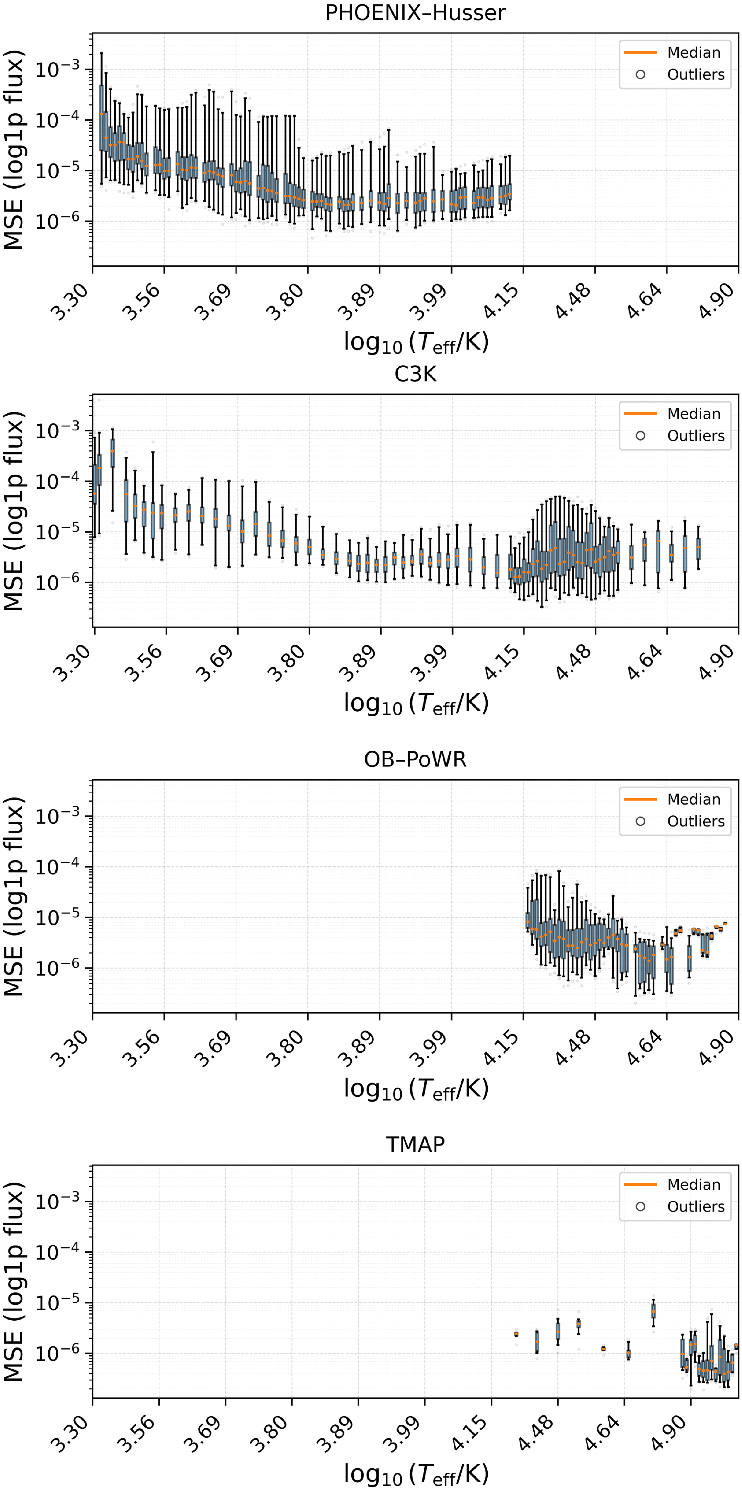
Figure 13. Long description
Panel A: Box plot for PHOENIX-Husser. The x-axis is labeled log10(Teff/K) ranging from 3.30 to 4.90, and the y-axis is labeled MSE (log1p flux) ranging from 10^-6 to 10^-3. The plot shows median values and outliers across different effective temperatures. Panel B: Box plot for C3K. The x-axis is labeled log10(Teff/K) ranging from 3.30 to 4.90, and the y-axis is labeled MSE (log1p flux) ranging from 10^-6 to 10^-3. The plot shows median values and outliers across different effective temperatures. Panel C: Box plot for OB–PoWR. The x-axis is labeled log10(Teff/K) ranging from 3.30 to 4.90, and the y-axis is labeled MSE (log1p flux) ranging from 10^-6 to 10^-3. The plot shows median values and outliers across different effective temperatures. Panel D: Box plot for TMAP. The x-axis is labeled log10(Teff/K) ranging from 3.30 to 4.90, and the y-axis is labeled MSE (log1p flux) ranging from 10^-6 to 10^-3. The plot shows median values and outliers across different effective temperatures.
Distribution of MSE across
 $\log g$
for the four libraries.
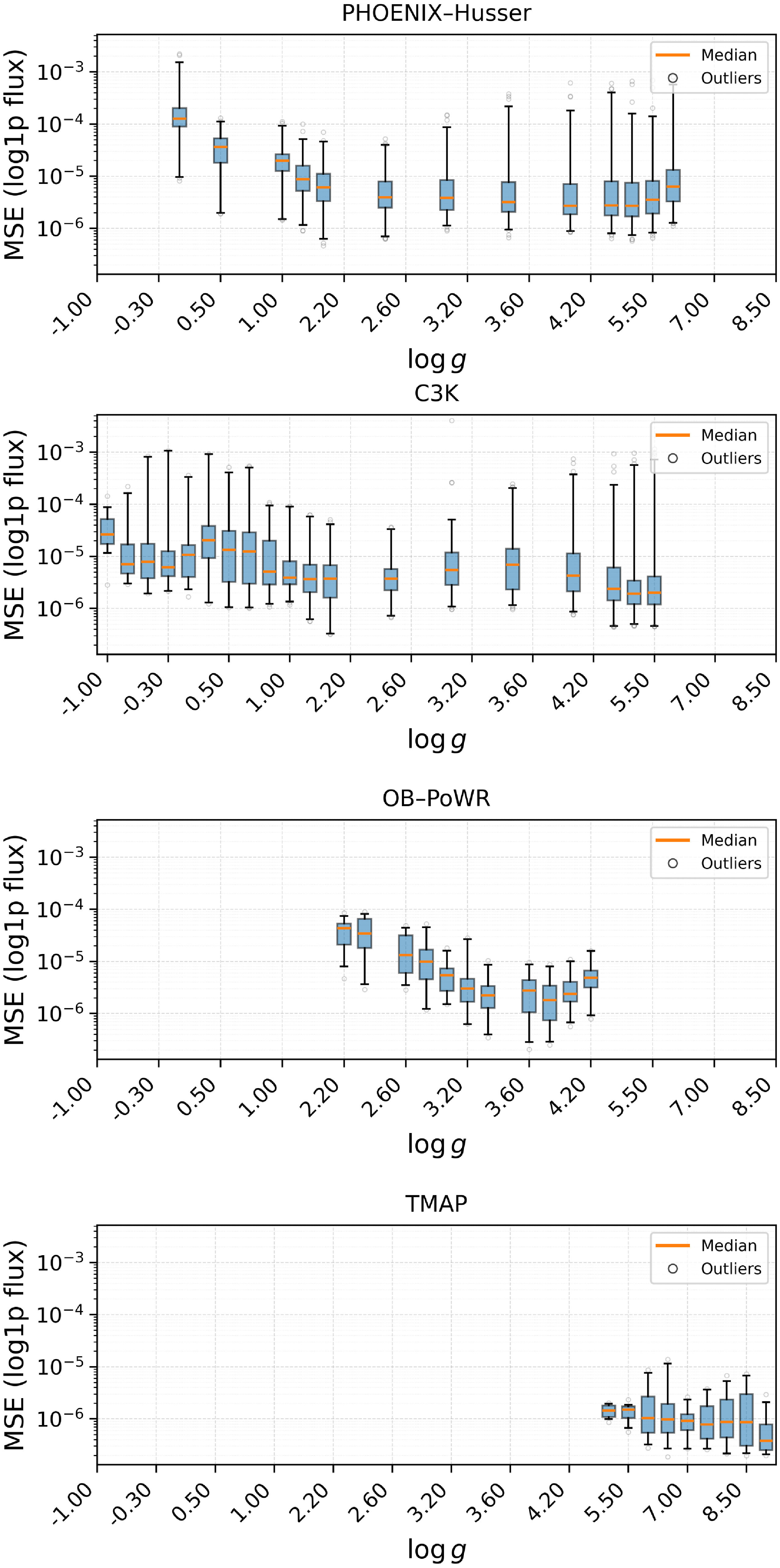
Figure 14. Long description
Panel A: The box plot for the PHOENIX-Husser library shows the distribution of mean squared error (MSE) in log1p flux across different values of log g. The x-axis represents log g values ranging from -1.00 to 8.50, and the y-axis represents MSE in log1p flux. The median MSE values are indicated by orange lines, and outliers are marked with gray circles. Panel B: The box plot for the C3K library shows the distribution of MSE in log1p flux across different values of log g. The x-axis represents log g values ranging from -1.00 to 8.50, and the y-axis represents MSE in log1p flux. The median MSE values are indicated by orange lines, and outliers are marked with gray circles. Panel C: The box plot for the OB–PoWR library shows the distribution of MSE in log1p flux across different values of log g. The x-axis represents log g values ranging from -1.00 to 8.50, and the y-axis represents MSE in log1p flux. The median MSE values are indicated by orange lines, and outliers are marked with gray circles. Panel D: The box plot for the TMAP library shows the distribution of MSE in log1p flux across different values of log g. The x-axis represents log g values ranging from -1.00 to 8.50, and the y-axis represents MSE in log1p flux. The median MSE values are indicated by orange lines, and outliers are marked with gray circles.
Distribution of MSE across
 $\log Z$
for the two libraries with metallicities.

The largest errors and most prominent outliers occur at the lowest temperatures, roughly
 $3.3 \lesssim \log_{10}\kern-1.5pt(T_{\mathrm{eff}}/\mathrm{K}) \lesssim 3.4$
. This behaviour is expected because cool-star spectra are intrinsically more difficult to model than hotter, smoother spectra. In this regime, the emergent spectrum is shaped by dense molecular absorption bands and broad, highly structured opacity features, rather than by a relatively smooth continuum with isolated atomic lines. Small changes in
 $\log_{10}\kern-1.5pt(T_{\mathrm{eff}}/\mathrm{K})$
,
 $\log g$
, or
 $\log Z$
can therefore produce comparatively large changes in the detailed spectral morphology. As a result, interpolation in this region is more demanding, particularly for a neural network that is required to learn a single smooth manifold across a non-uniform multi-library grid.
The increased low-temperature error should therefore not be interpreted as a generic failure of SM-Net, but as a reflection of the difficulty of this part of the training domain. The lowest-temperature region is dominated by PHOENIX–Husser and C3K spectra, where the library coverage is non-uniform and the two libraries can differ substantially at neighbouring locations in the parameter grid. These differences arise from distinct atmosphere assumptions, opacity treatments, and line lists, and they are consistent with the cross-library residuals discussed in Section 5. Consequently, SM-Net is forced to learn a continuous representation through a region where the reference spectra themselves are more structured and less mutually consistent. Elevated outlier rates are also seen near library-overlap boundaries, especially around the PHOENIX–Husser/C3K transition. By contrast, regions dominated by a single internally consistent library, such as the hottest TMAP regime or the most metal-poor PHOENIX–Husser bins, show uniformly low errors and minimal scatter.
The per-library breakdown supports this interpretation. For
 $\log_{10}\kern-1.5pt(T_{\mathrm{eff}}/\mathrm{K})$
, the largest reconstruction errors at low temperature are concentrated in the PHOENIX–Husser and C3K libraries, which dominate the cool-star regime and contain strong molecular structure as well as library-dependent differences at fixed
 $(T_{\mathrm{eff}},\log g,\log Z)$
. At higher temperatures, where OB–PoWR and TMAP dominate, the MSE remains generally lower and prominent outliers are less common. For
 $\log g$
, the highest mean errors occur near
 $\log g=0$
for PHOENIX–Husser, where the MSE exceeds
 $\sim$
 $10^{-4}$
, while the corresponding C3K errors remain close to
 $\sim$
 $10^{-5}$
around
 $\log g=0$
. This reflects the denser local sampling of C3K in this region, which causes the learned manifold to follow the C3K spectral behaviour more closely and increases the residuals relative to the retained PHOENIX–Husser references. For
 $\log Z$
, the mean MSE remains broadly uniform across the two libraries with explicit metallicity coverage, with outliers dispersed rather than concentrated in any particular metallicity bin.
6.2. Synthetic broad-band colour and line-strength validation
The MSE values reported in Table 4 quantify reconstruction accuracy directly in the log1p-scaled flux representation used for training and evaluation. While this provides a measure of pixel-level spectral agreement, many astronomical applications rely on derived observables rather than individual flux samples. We therefore extend the validation in two complementary directions: synthetic broad-band colours, which probe the integrated spectral energy distribution over wide wavelength intervals, and line-strength indices, which probe the reconstruction of narrower spectral features.
Synthetic photometry is commonly used to evaluate stellar model fluxes, broad-band colours, and bolometric corrections (Casagrande & VandenBerg 2014). For this analysis, the spectra were transformed back to direct flux space using the inverse of the log1p scaling described in Section 2. Synthetic colours were then computed from band-averaged
 $F_\nu$
values using filter response curves from the Spanish Virtual Observatory (SVO) Filter Profile Service, an online repository of standardised photometric filter transmission curves (Rodrigo et al. Reference Rodrigo, Solano and Bayo2012, Reference Rodrigo2024; Rodrigo & Solano Reference Rodrigo and Solano2020). All colours are reported in the AB magnitude system, in which magnitudes are defined relative to a constant reference flux density per unit frequency.
We considered the colours
 $g-r$
,
 $r-i$
,
 $g-i$
, and
 $J-K_s$
. The first two probe adjacent optical bands,
 $g-i$
provides a broader optical baseline, and
 $J-K_s$
probes the near-infrared spectral shape. Together, the
 $(\,g-i)$
versus
 $(J-K_s)$
plane provides a combined optical and near-infrared colour–colour diagnostic. We use
 $K_s$
rather than the classical broad K band because it avoids the more problematic long-wavelength portion of the K response. The selected bands are representative of SDSS-like optical and 2MASS near-infrared photometry (Doi et al. Reference Doi2010; Skrutskie et al. Reference Skrutskie2006).
Figure 16 compares the retained test-set spectra and the corresponding SM-Net predictions in the
 $(\,g-i)$
versus
 $(J-K_s)$
plane. The contours are constructed from the full test set using a
 $42\times42$
two-dimensional histogram, lightly smoothed with a Gaussian kernel of width one histogram bin. They delineate the highest-density regions containing 50%, 80%, and 95% of the corresponding smoothed distribution, shown by the solid red, dashed blue, and dotted black contours, respectively. The same binning, smoothing, and colour–colour limits are applied to the reference and SM-Net distributions. The faint individual points are subsampled only for visual clarity and do not affect the contour calculation.
Test-set colour–colour distributions in the
 $(\,g-i)_{\text{AB}}$
versus
 $(J-K_s)_{\text{AB}}$
plane for the retained reference spectra (left) and the corresponding SM-Net predictions (right). The Sun-like validation point is overlaid for reference. The solid red, dashed blue, and dotted black contours enclose, respectively, the highest-density regions containing 50%, 80%, and 95% of each smoothed distribution. The orange marker denotes the Sun-like validation point at
 $T_{\text{eff}}=5\,800\,$
K,
 $\log g=4.5$
, and
 $\log Z=0$
.
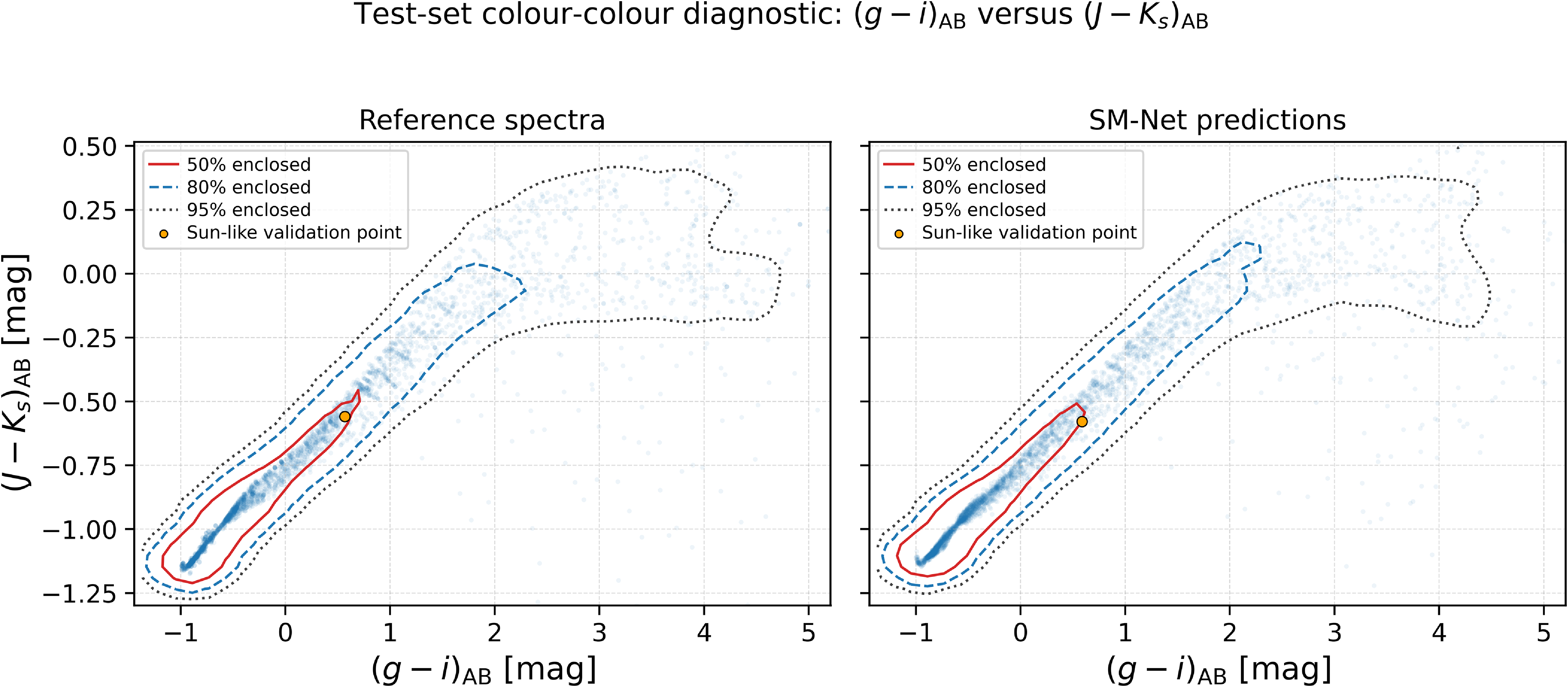
A Sun-like spectrum from the validation set is manually overlaid on both panels as an additional reference point. The corresponding SM-Net prediction lies close to the PHOENIX–Husser validation spectrum in colour–colour space. Figure 16 therefore provides a qualitative comparison of the global colour distributions, while the residual-based comparisons below quantify their reconstruction accuracy directly.
To quantify the colour-reconstruction precision directly, Figure 17 shows the residuals for
 $g-r$
,
 $r-i$
,
 $g-i$
, and
 $J-K_s$
as a function of
 $\log_{10}\kern-1.5pt(T_{\mathrm{eff}}/\mathrm{K})$
over the full test set. The running medians remain close to zero over most of the sampled temperature range, indicating little systematic colour bias, while the scatter increases towards the cooler end of the grid. The median absolute residuals are 0.022, 0.012, 0.028, and 0.015 mag for
 $g-r$
,
 $r-i$
,
 $g-i$
, and
 $J-K_s$
, respectively, with corresponding 90th-percentile absolute residuals of 0.070, 0.046, 0.077, and 0.063 mag. This full-test-set diagnostic complements Figure 16 by showing directly where the broad-band reconstruction errors occur in stellar-parameter space.
Synthetic broad-band colour residuals across the full test set as a function of effective temperature. Residuals are defined as
 $\Delta(X-Y)=(X-Y)_{\text{reference}}-(X-Y)_{\text{SM-Net}}$
. The faint points show individual test spectra, while the solid line shows the running median and the shaded region denotes the 16–84 percentile interval. The median absolute residual and 90th-percentile absolute residual are reported in each panel.
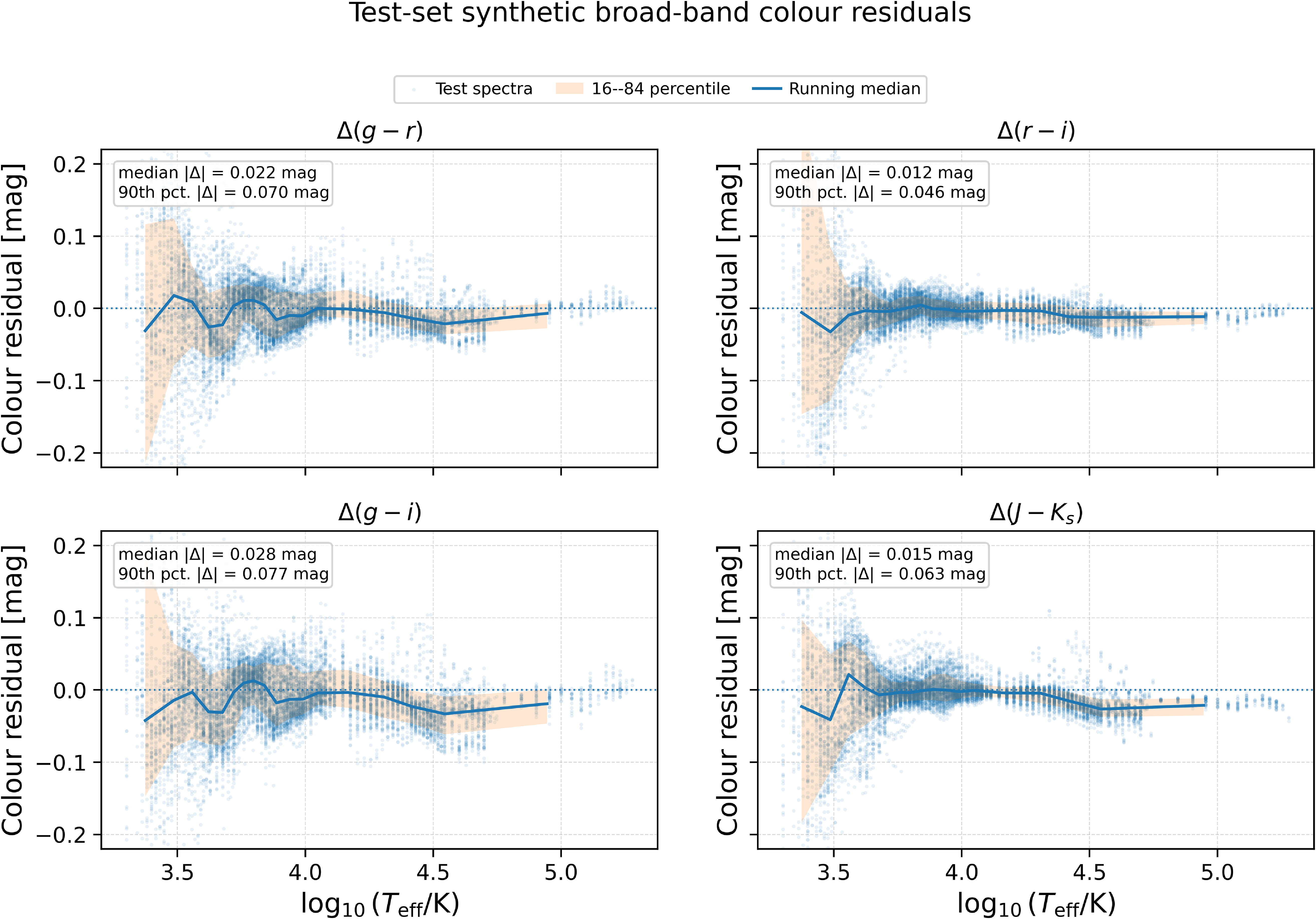
Figure 17. Long description
Panel A: A scatter plot shows color residual in magnitudes for the color index g-r as a function of the logarithm of effective temperature in Kelvin. The faint points represent individual test spectra, while the solid blue line shows the running median and the shaded orange region denotes the 16-84 percentile interval. The median absolute residual is 0.022 mag, and the 90th percentile absolute residual is 0.070 mag. Panel B: A scatter plot shows color residual in magnitudes for the color index r-i as a function of the logarithm of effective temperature in Kelvin. The faint points represent individual test spectra, while the solid blue line shows the running median and the shaded orange region denotes the 16-84 percentile interval. The median absolute residual is 0.012 mag, and the 90th percentile absolute residual is 0.046 mag. Panel C: A scatter plot shows color residual in magnitudes for the color index g-i as a function of the logarithm of effective temperature in Kelvin. The faint points represent individual test spectra, while the solid blue line shows the running median and the shaded orange region denotes the 16-84 percentile interval. The median absolute residual is 0.028 mag, and the 90th percentile absolute residual is 0.077 mag. Panel D: A scatter plot shows color residual in magnitudes for the color index J-Ks as a function of the logarithm of effective temperature in Kelvin. The faint points represent individual test spectra, while the solid blue line shows the running median and the shaded orange region denotes the 16-84 percentile interval. The median absolute residual is 0.015 mag, and the 90th percentile absolute residual is 0.063 mag.
For the quantitative comparison with the intrinsic differences between stellar libraries, we next restrict the analysis to the 783 exact
 $(T_{\mathrm{eff}},\log g,\log Z)$
labels shared by PHOENIX–Husser and C3K. At each label, colours were calculated for the PHOENIX–Husser spectrum, the C3K spectrum, and the corresponding SM-Net prediction. This provides two directly comparable residual measurements over an identical stellar-parameter sample: PHOENIX–Husser versus C3K, which characterises the underlying cross-library variation, and PHOENIX–Husser versus SM-Net, which measures the additional reconstruction difference introduced by the model.
Using PHOENIX–Husser as the common reference, we define the PHOENIX–Husser/SM-Net colour difference as
 \begin{equation}\Delta_{\textrm {H-SM}}(X-Y) =(X-Y)_{\textrm {PHOENIX-Husser}}-(X-Y)_{\textrm {SM-Net}},\end{equation}
and the corresponding PHOENIX–Husser/C3K difference as
 \begin{equation}\Delta_{\textrm {H-C3K}}(X-Y) =(X-Y)_{\textrm {PHOENIX-Husser}}-(X-Y)_{\textrm {C3K}}.\end{equation}
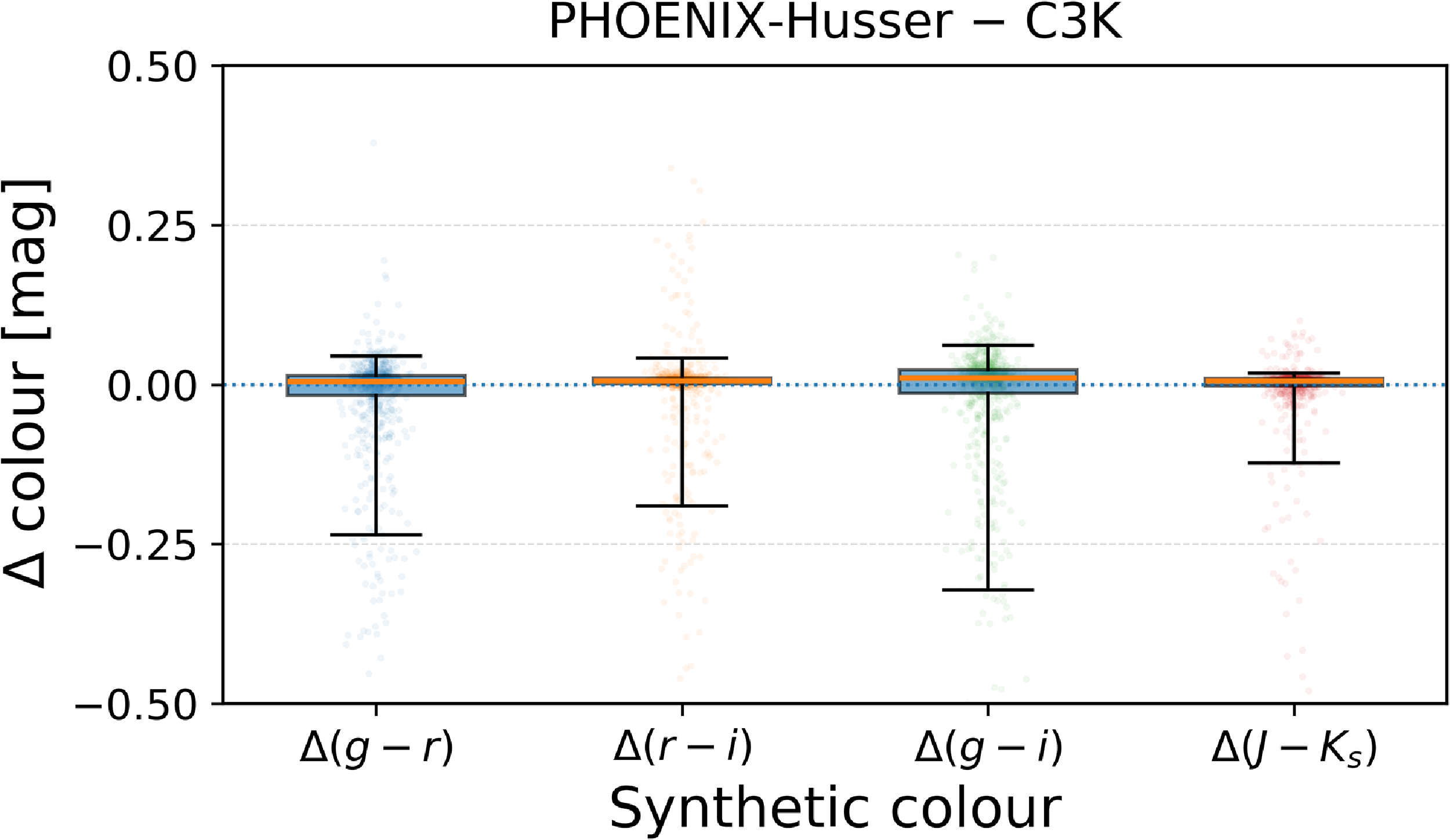
A positive difference indicates that the PHOENIX–Husser colour is redder than the comparison colour, while a negative difference indicates that it is bluer. Both box plots are displayed over the common range
 $-0.5$
to
 $0.5$
mag for visual comparison. Values outside this displayed range remain included in the summary statistics.
Figure 18 shows that measurable library-to-library colour differences remain even when
 $T_{\mathrm{eff}}$
,
 $\log g$
, and
 $\log Z$
are identical. The PHOENIX–Husser/C3K distributions contain extended, predominantly negative tails, with the largest 90th-percentile absolute difference occurring for
 $g-i$
. These differences provide a reference scale for interpreting the corresponding SM-Net reconstruction residuals.
Figure 19 shows the PHOENIX–Husser/SM-Net differences over the same 783 labels. The signed medians remain close to zero, indicating little systematic colour bias, although the central SM-Net distributions are broader than the corresponding PHOENIX–Husser/C3K distributions.
To place the differences in the context of observational uncertainty, we used the band-level fractional flux error floors listed in Table 1 of Bellstedt et al. (Reference Bellstedt2020). These were converted to approximate magnitude uncertainties and the corresponding colour floor was calculated by adding the two band-level terms in quadrature:
 \begin{equation}\sigma_{X-Y} =\frac{2.5}{\ln 10}\sqrt{f_X^2+f_Y^2},\end{equation}
where
 $f_X$
and
 $f_Y$
are the fractional flux error floors in the two bands.
Synthetic colour differences, defined as PHOENIX–Husser
 $-$
C3K, at the 783 exact matched stellar-parameter labels.
Synthetic colour differences, defined as PHOENIX–Husser
 $-$
SM-Net, at the same 783 matched stellar-parameter labels.
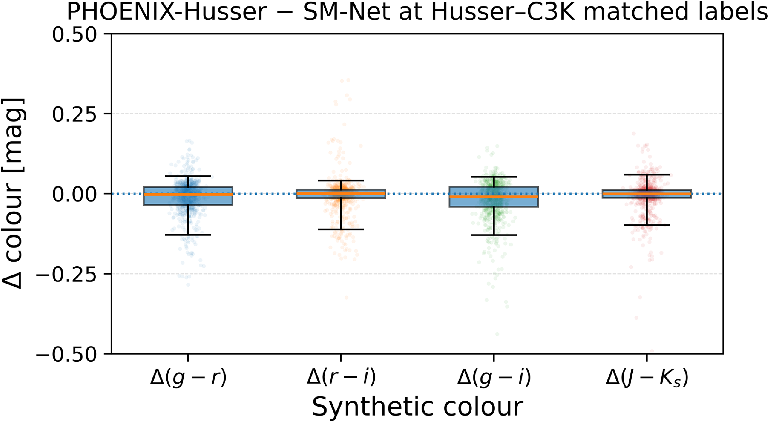
Table 5 separates the typical differences, represented by the median absolute residual, from the upper-tail behaviour represented by the 90th percentile. The median absolute PHOENIX–Husser/C3K differences are smaller than the corresponding PHOENIX–Husser/SM-Net values for all four colours. For example, the median absolute
 $g-i$
differences are 0.0217 and 0.0307 mag, respectively. Conversely, the 90th-percentile SM-Net differences for
 $g-r$
,
 $r-i$
, and
 $g-i$
are smaller than the corresponding PHOENIX–Husser/C3K values, indicating less extended optical tails. For
 $J-K_s$
, SM-Net shows both a larger median absolute difference and a larger 90th-percentile difference than C3K, although its 90th-percentile value of 0.0787 mag remains below the adopted observational floor of 0.0997 mag. Overall, the matched-label comparison indicates that SM-Net does not simply reproduce either input library. Its central colour residuals are somewhat broader than the PHOENIX–Husser/C3K differences, while its extreme optical residuals are less extended.
Typical and upper-tail synthetic-colour differences at the 783 exact PHOENIX–Husser/C3K matched labels. Differences are defined relative to PHOENIX–Husser. The median absolute difference characterises the typical offset, while the 90th percentile characterises the upper tail. All values are in magnitudes.
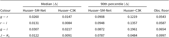
Table 5. Long description
A table comparing synthetic-colour differences at matched labels. The table has four rows and six columns. Column headers are Median |Δ| Husser-SM-Net, Median |Δ| Husser-C3K, 90th percentile |Δ| Husser-SM-Net, 90th percentile |Δ| Husser-C3K, and Obs. floor. Row labels are g - r, r - i, g - i, and J - Ks. Row 1: Median |Δ| Husser-SM-Net, 0.0260; Median |Δ| Husser-C3K, 0.0147; 90th percentile |Δ| Husser-SM-Net, 0.0908; 90th percentile |Δ| Husser-C3K, 0.1219; Obs. floor, 0.0543. Row 2: Median |Δ| Husser-SM-Net, 0.0131; Median |Δ| Husser-C3K, 0.0084; 90th percentile |Δ| Husser-SM-Net, 0.0948; 90th percentile |Δ| Husser-C3K, 0.1357; Obs. floor, 0.0587. Row 3: Median |Δ| Husser-SM-Net, 0.0307; Median |Δ| Husser-C3K, 0.0217; 90th percentile |Δ| Husser-SM-Net, 0.0872; 90th percentile |Δ| Husser-C3K, 0.1961; Obs. floor, 0.0654. Row 4: Median |Δ| Husser-SM-Net, 0.0122; Median |Δ| Husser-C3K, 0.0091; 90th percentile |Δ| Husser-SM-Net, 0.0787; 90th percentile |Δ| Husser-C3K, 0.0484; Obs. floor, 0.0997.
Comparison of line-strength indices from the reference test spectra and the corresponding SM-Net reconstructions for H
 $\beta$
, Fe5270, Fe5335, Ca4227, CN1, and TiO2. Atomic indices are given as pseudo-equivalent widths in Å, and CN1 and TiO2 in magnitudes. Points are coloured by
 $\log_{10}\kern-1.5pt(T_{\text{eff}}/\text{K})$
, with the dashed line indicating one-to-one agreement. Each panel reports r,
 $R^2$
, the median absolute residual, and the 90th percentile of the absolute residual.
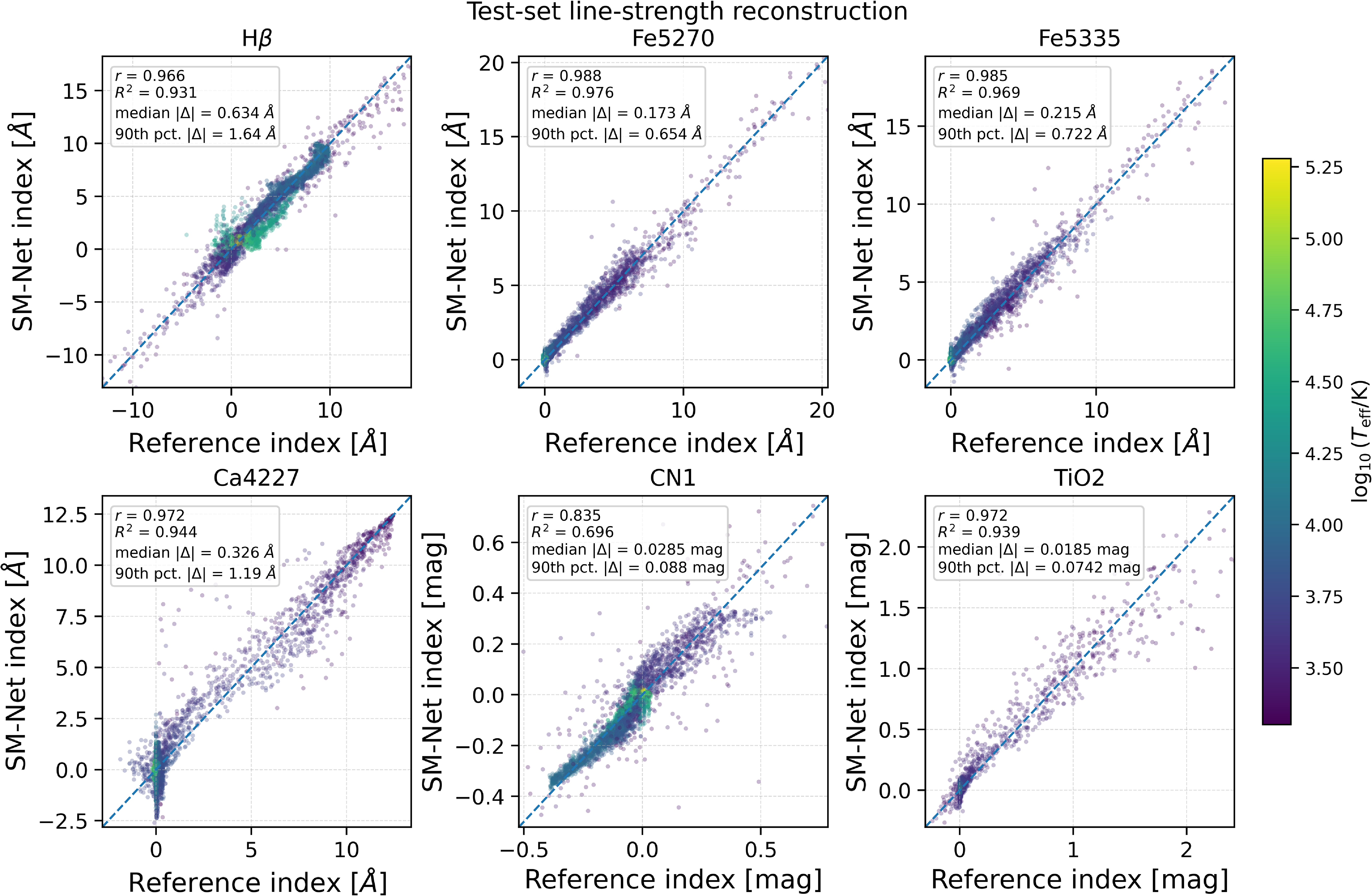
Figure 20. Long description
Panel Hβ: A scatter plot compares the SM-Net index with the Reference index for Hβ. The x-axis is labeled ’Reference index [Å]’ and the y-axis is labeled ’SM-Net index [Å]’. The plot includes a dashed line indicating one-to-one agreement. Panel Fe5270: A scatter plot compares the SM-Net index with the Reference index for Fe5270. The x-axis is labeled ’Reference index [Å]’ and the y-axis is labeled ’SM-Net index [Å]’. The plot includes a dashed line indicating one-to-one agreement. Panel Fe5335: A scatter plot compares the SM-Net index with the Reference index for Fe5335. The x-axis is labeled ’Reference index [Å]’ and the y-axis is labeled ’SM-Net index [Å]’. The plot includes a dashed line indicating one-to-one agreement. Panel Ca4227: A scatter plot compares the SM-Net index with the Reference index for Ca4227. The x-axis is labeled ’Reference index [Å]’ and the y-axis is labeled ’SM-Net index [Å]’. The plot includes a dashed line indicating one-to-one agreement. Panel CN1: A scatter plot compares the SM-Net index with the Reference index for CN1. The x-axis is labeled ’Reference index [mag]’ and the y-axis is labeled ’SM-Net index [mag]’. The plot includes a dashed line indicating one-to-one agreement. Panel TiO2: A scatter plot compares the SM-Net index with the Reference index for TiO2. The x-axis is labeled ’Reference index [mag]’ and the y-axis is labeled ’SM-Net index [mag]’. The plot includes a dashed line indicating one-to-one agreement. Each panel reports r, R², the median absolute residual, and the 90th percentile of the absolute residual.
Broad-band colours primarily test the integrated spectral energy distribution and can remain accurate even when individual absorption features are imperfectly reconstructed. We therefore performed a complementary test using representative line-strength diagnostics over the full test set. The selected indices comprise the Balmer H
 $\beta$
feature, the Fe5270 and Fe5335 iron indices, Ca4227, and the molecular CN1 and TiO2 indices, thereby sampling hydrogen, metal, calcium, and molecular absorption features. The central feature bands used are 4847.875–4876.625 Å for H
 $\beta$
, 5245.650–5285.650 Å for Fe5270, 5312.125–5352.125 Å for Fe5335, 4222.250–4234.750 Å for Ca4227, 4142.125–4177.125 Å for CN1, and 6189.625–6272.125 Å for TiO2.
The atomic indices are measured as pseudo-equivalent widths in Å, whereas CN1 and TiO2 are measured in magnitudes. Identical feature and pseudo-continuum passbands are applied to each reference spectrum and its corresponding SM-Net reconstruction after transformation back to direct flux space. The pseudo-continuum is estimated from the blue and red sidebands surrounding each feature. Consequently, a negative atomic index indicates that the flux within the feature band lies, on average, above this fitted pseudo-continuum and does not by itself imply physical line emission. The line-strength residual is defined as
 $\Delta I=I_{\textrm {reference}}-I_{\textrm {SM-Net}}$
. The
 $R^2$
values shown in Figure 20 quantify agreement with exact one-to-one prediction rather than being defined simply as the square of the Pearson correlation coefficient. These diagnostics test the spectral features present in the underlying theoretical stellar libraries. They do not include additional line production associated with circumstellar or nebular gas and dust, which would require separate physical post-processing.
Figure 20 compares the indices measured from the reference spectra with those measured from the SM-Net reconstructions. The statistics in each panel are calculated using the full set of valid test spectra; the displayed points are subsampled only for visual clarity. Five of the six diagnostics show strong agreement with the one-to-one relation, with
 $R^2=0.931$
–
 $0.976$
for H
 $\beta$
, Fe5270, Fe5335, Ca4227, and TiO2. CN1 is less tightly reconstructed, with
 $R^2=0.696$
. For the atomic indices, the median absolute residual ranges from 0.173 Å for Fe5270 to 0.634 Å for H
 $\beta$
; the corresponding median absolute residuals for CN1 and TiO2 are 0.0285 and 0.0185 mag. The temperature colouring also reveals parameter-dependent behaviour, with some of the larger deviations in the metal and molecular diagnostics associated with cooler spectra.
Additional per-library checks show that the behaviour is not uniform across the four input libraries. PHOENIX–Husser and C3K show strong line-index reconstruction, including the negative H
 $\beta$
branch already present in their reference spectra. TMAP also shows good H
 $\beta$
reconstruction, while several of its other indices span only a very small intrinsic range. The main weaker regime is OB–PoWR, particularly for H
 $\beta$
. This is consistent with the irregular spectral behaviour already identified during dataset quality control, where a subset of OB–PoWR spectra with strong discontinuities and abrupt continuum changes was removed. Even among the retained spectra, comparatively sharp local structure remains in some regions and is more difficult for SM-Net to reconstruct.
Appendix Figures A1 and A2 illustrate these effects directly. The first set of plots show the most extreme reference H
 $\beta$
case from each library together with the fitted pseudo-continuum, demonstrating how strong negative indices can arise in highly structured spectra. The second figure shows representative non-extreme cases in which both the H
 $\beta$
index and the local feature shape are reconstructed well, while also illustrating the greater difficulty of the OB–PoWR regime.
Taken together, the broad-band and line-strength analyses extend the evaluation beyond pixel-level MSE and test quantities that are more directly relevant to downstream astronomical applications. SM-Net reproduces the overall broad-band colour distributions with small systematic offsets and tracks several commonly used line-strength diagnostics closely, while the residual distributions, the weaker CN1 reconstruction, and the more challenging OB–PoWR line-index behaviour identify regimes in which additional uncertainty remains. These results therefore demonstrate both the utility and the current limitations of the learned spectral manifold for applications that depend on integrated colours or individual spectral features.
6.3. Reconstructed spectra
In this section, we present representative spectra reconstructed by SM-Net. The Sun-like example is drawn from the validation set, whereas the remaining examples are drawn from the test set. The validation example was not used for gradient-based training, while the test examples were not used during either training or checkpoint selection. All spectra are shown in the log1p-scaled flux representation used for training and evaluation. In each example, the upper panel shows the reference and SM-Net spectra, while the lower panel shows the residual, defined as reference
 $-$
SM-Net. The plotted axes are linear in this transformed flux space.
Figure 21 shows the spectrum in the combined dataset that is closest to the Sun, with parameters
 $T_{\mathrm{eff}} = 5\,800\,\mathrm{K}$
,
 $\log g = 4.5$
, and
 $\log Z = 0$
. This spectrum belongs to the validation set, and the prediction shown was generated using the best-validation checkpoint at epoch 389. The SM-Net prediction closely matches the corresponding PHOENIX–Husser template at the same parameter values. Most of the residual structure appears at shorter wavelengths; however, the peak deviations remain below
 $\sim$
 $0.02$
in log1p-scaled flux, corresponding to less than 2% of the maximum normalised flux value of 1 in the transformed representation.
Predicted spectrum for the closest Sun-like grid point, compared with the corresponding PHOENIX–Husser reference spectrum. The upper panel shows the spectra in log1p-scaled flux space, and the lower panel shows the residual, defined as reference
 $-$
SM-Net.

High-fidelity SM-Net reconstruction for
 $T_{\text{eff}} = 6\,900\,\text{K}$
,
 $\log g = 4.0$
, and
 $\log Z = -2.0$
, shown against the corresponding PHOENIX–Husser reference spectrum.
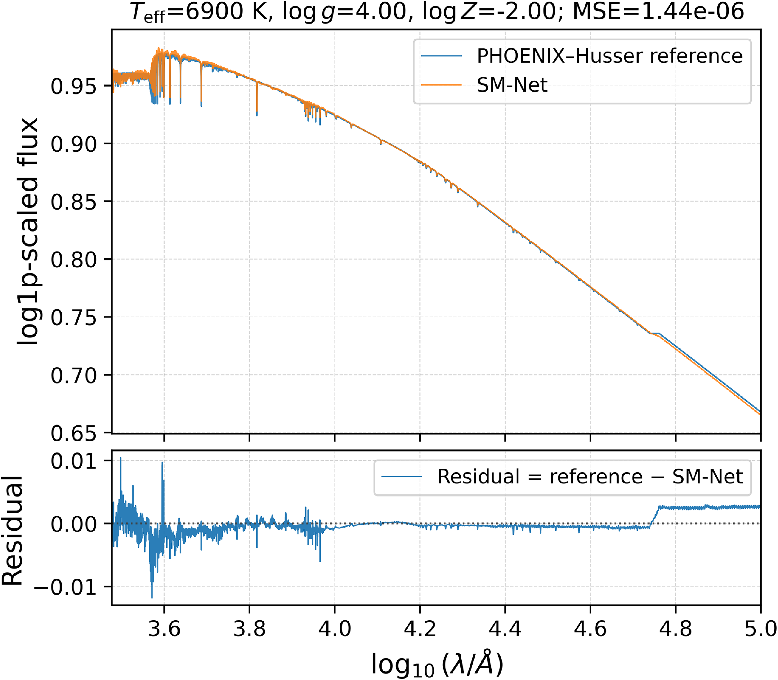
Figure 22 shows the SM-Net reconstruction for a star with
 $T_{\mathrm{eff}}=6{\,}900\,\mathrm{K}$
,
 $\log g=4.0$
, and
 $\log Z=-2.0$
. The model accurately reproduces the fine spectral structure, achieving a mean-squared error of
 $1.44\times10^{-6}$
relative to the PHOENIX–Husser reference spectrum. This example illustrates the high reconstruction accuracy achieved in this region of parameter space.
Figure 23 presents another high-quality reconstruction, this time for a hotter star with
 $T_{\mathrm{eff}}=13{\,}000\,\mathrm{K}$
,
 $\log g=4.5$
, and
 $\log Z=-1.5$
. SM-Net reproduces the detailed spectral structure with a mean-squared error of
 $9.67\times10^{-7}$
relative to the corresponding C3K reference spectrum. Together, Figures 22 and 23 provide high-quality examples drawn from two different constituent libraries.
Figure 24 shows an example of a poor-quality reconstruction for
 $T_{\mathrm{eff}} = 2\,200\,\mathrm{K}$
,
 $\log g = 3.0$
, and
 $\log Z = -2.1$
, compared against the corresponding C3K reference spectrum. The model exhibits substantial residuals across the full wavelength range, with the largest deviations occurring at shorter wavelengths. This case highlights the greater difficulty of accurately reconstructing spectra in the very low–temperature regime.
High-quality SM-Net reconstruction for
 $T_{\text{eff}} = 13{\,}000\,\text{K}$
,
 $\log g = 4.5$
, and
 $\log Z = -1.5$
, compared with the corresponding C3K reference spectrum.
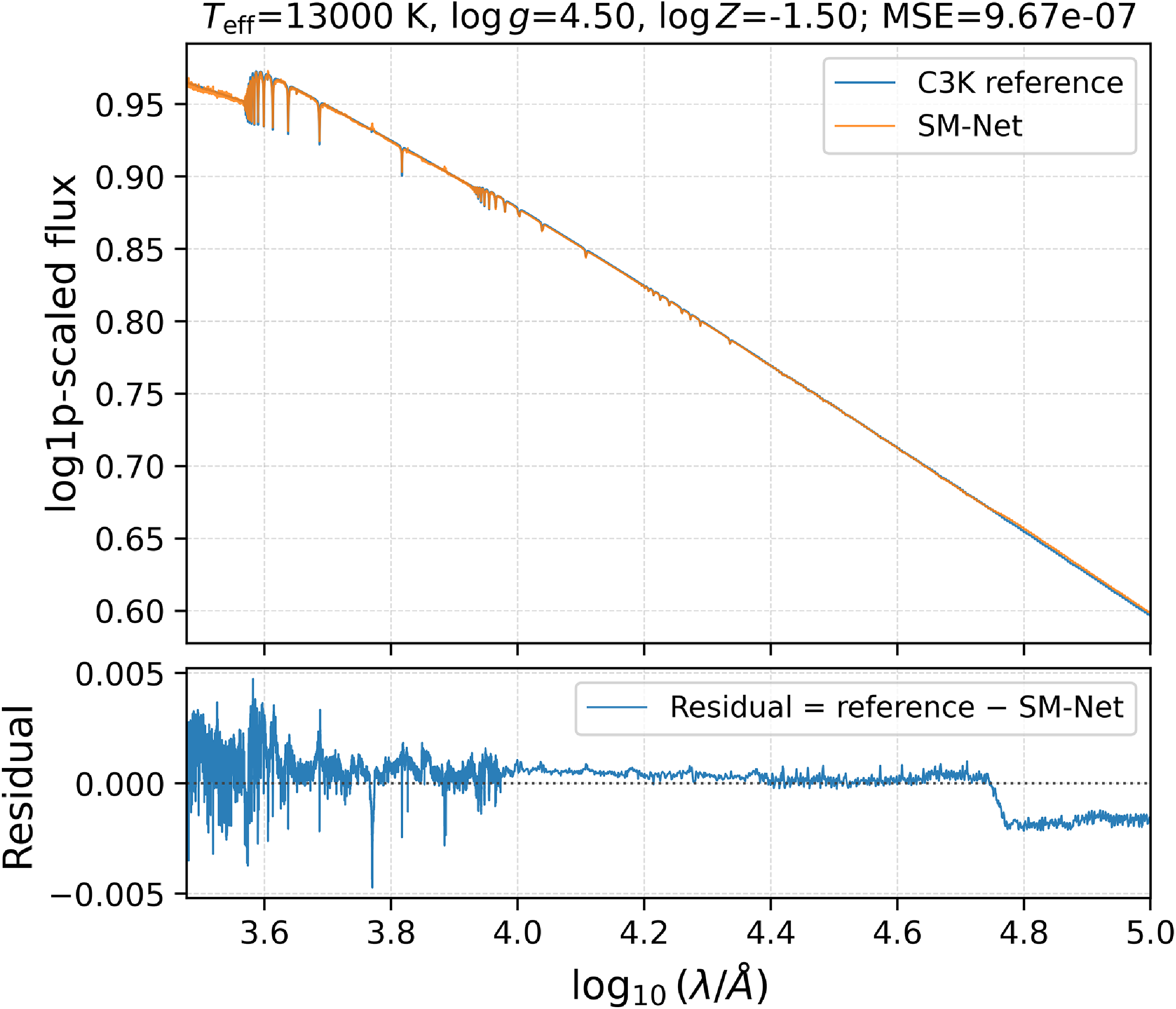
Example of a low-quality reconstruction at
 $T_{\text{eff}} = 2\,200\,\text{K}$
,
 $\log g = 3.0$
, and
 $\log Z = -2.1$
, shown against the corresponding C3K reference spectrum.
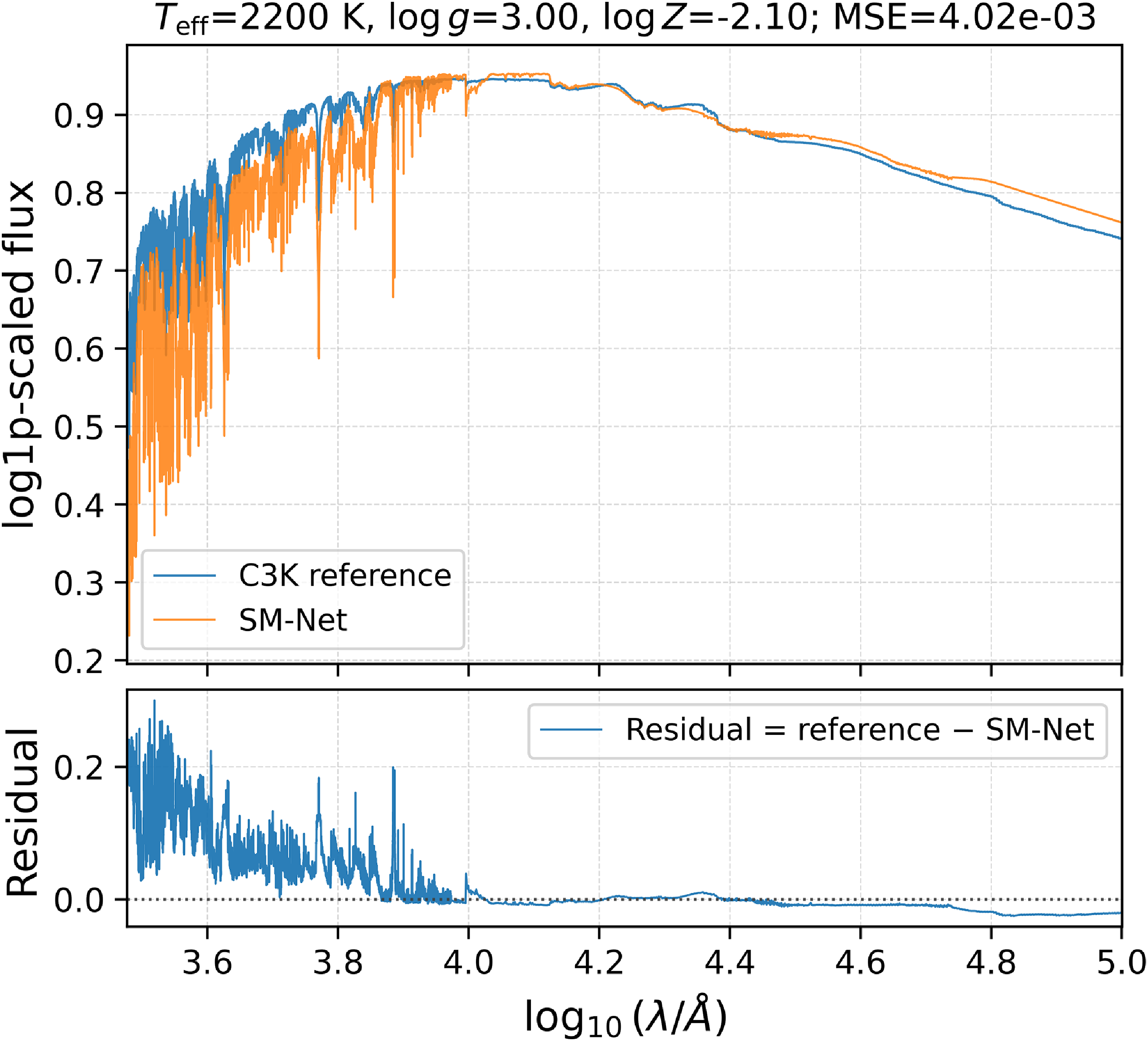
Figure 25 presents another example of a low-quality reconstruction for
 $T_{\mathrm{eff}}=22{\,}000\,\mathrm{K}$
,
 $\log g=2.4$
, and
 $\log Z=-1.0$
, compared with the corresponding OB–PoWR reference spectrum. SM-Net struggles to reproduce both the spectral features and the overall wavelength-dependent slope, with the residual reaching approximately 0.04 in the normalised log1p-scaled flux representation at the longest wavelengths. This example illustrates the difficulty of modelling regions in which sparse library coverage makes interpolation particularly challenging.
Example of a low-quality reconstruction for
 $T_{\text{eff}} = 22\,000\,\text{K}$
,
 $\log g = 2.4$
, and
 $\log Z = -1.0$
, compared against the corresponding OB–PoWR reference spectrum.
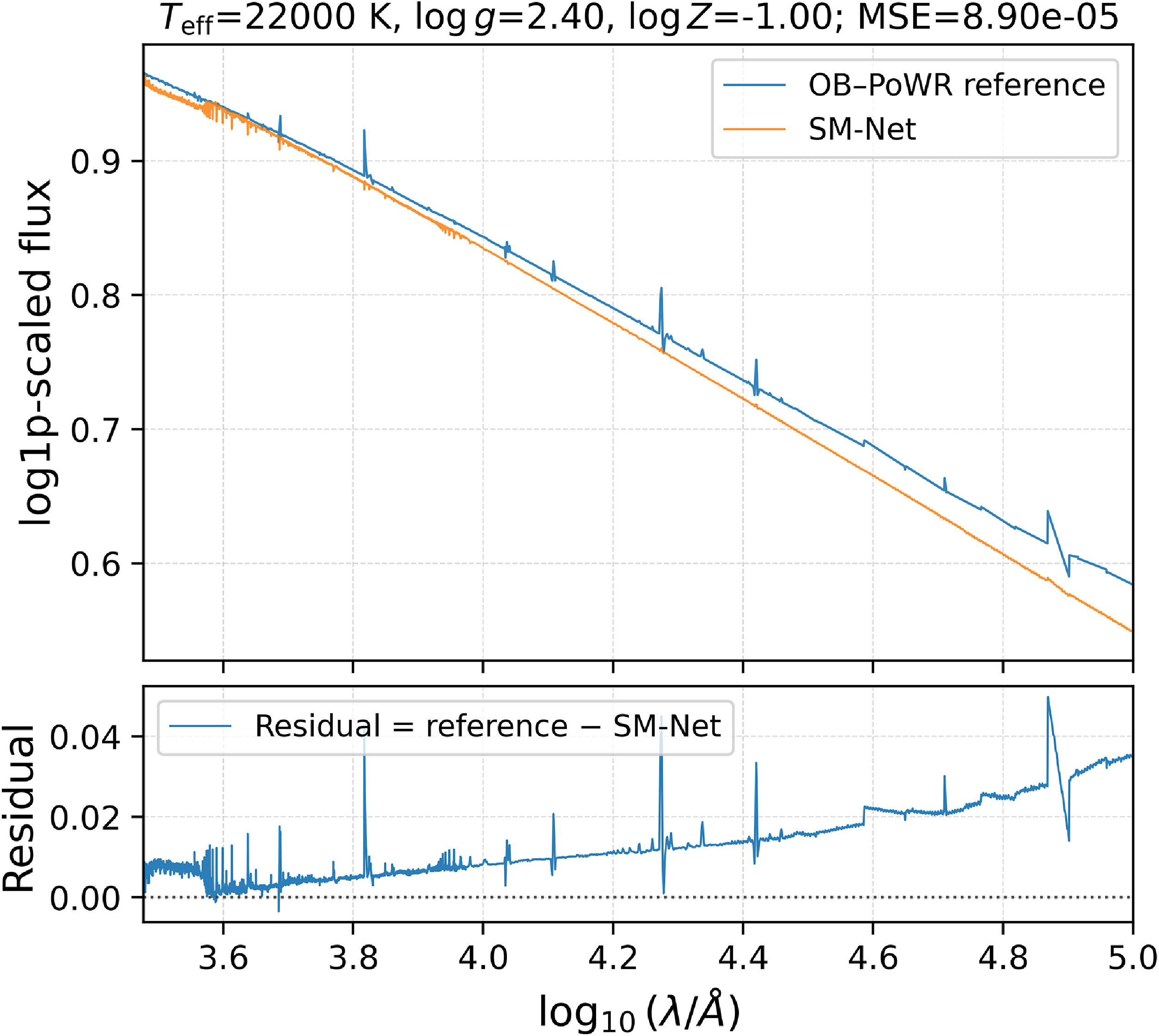
Example of SM-Net reconstructing the missing high-wavelength flux for
 $T_{\text{eff}} = 60{\,}000\,\text{K}$
and
 $\log g = 6.5$
, compared with the corresponding TMAP reference spectrum.
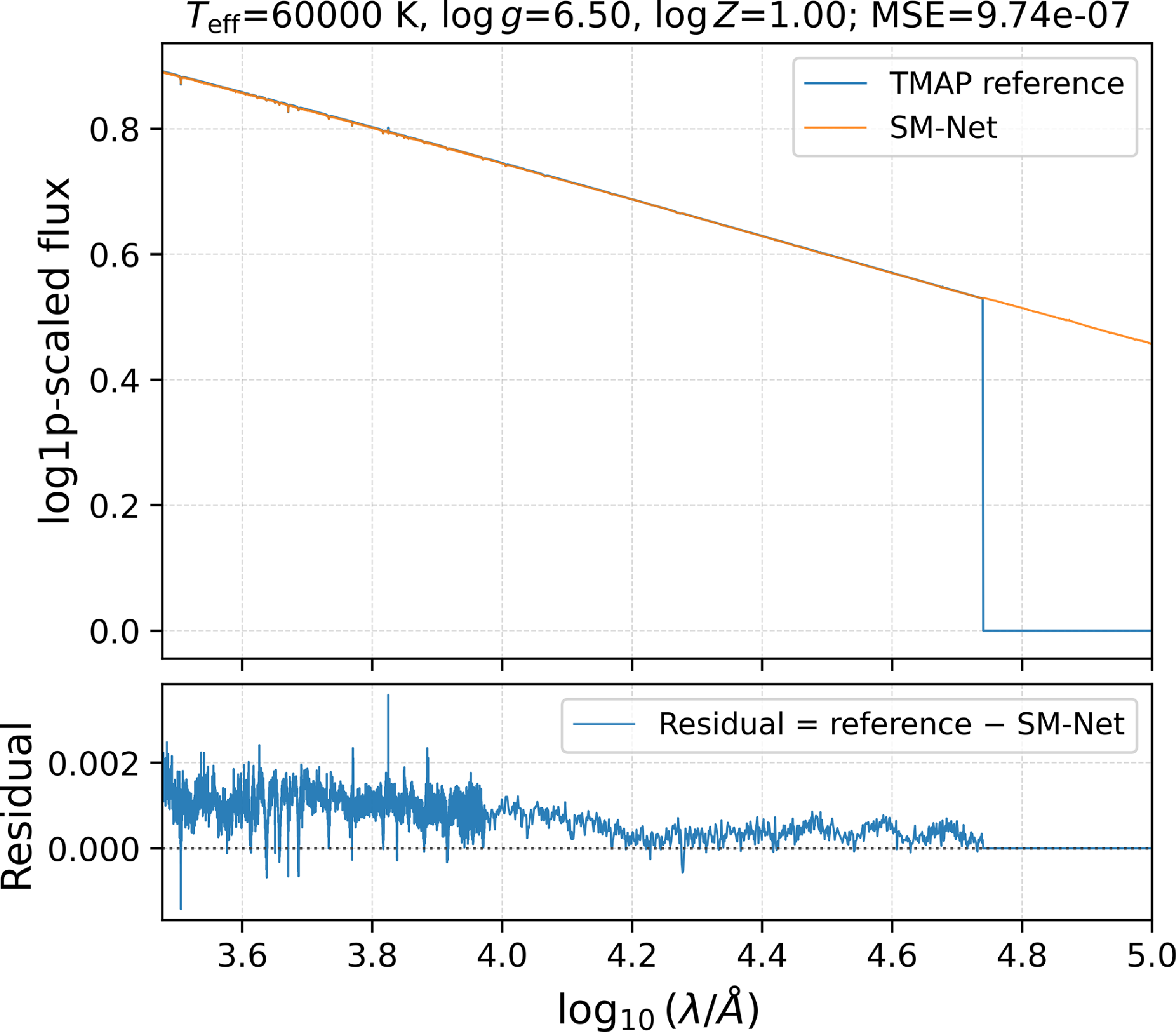
Figure 26, corresponding to
 $T_{\mathrm{eff}}=60{\,}000\,\mathrm{K}$
,
 $\log g=6.5$
, and an assigned
 $\log Z=1.0$
, illustrates SM-Net’s reconstruction of a masked high-wavelength region in a TMAP spectrum. The model continues the spectral trend through the region in which the reference flux is unavailable while remaining consistent with the surrounding continuum. Because TMAP does not explicitly parametrise metallicity, the assigned
 $\log Z$
value serves only to embed the spectrum in the common three-parameter grid. This example demonstrates how SM-Net uses correlations learned from neighbouring grid points to infer a smooth continuation through a masked wavelength interval.
Across these examples, reconstruction quality is strongly dependent on the local spectral regime. The best PHOENIX–Husser, C3K, and TMAP cases achieve MSE values of approximately
 $10^{-6}$
, demonstrating that SM-Net can reproduce both continuum shape and detailed spectral features with high accuracy in well-represented regions of the grid. The contrasting low-quality examples show that errors increase in sparsely sampled or physically complex regimes, particularly at very low temperatures and near difficult library boundaries. The TMAP example additionally demonstrates that the learned model can infer a smooth continuation through wavelength regions masked in the reference spectrum. These results are consistent with the parameter-dependent error distributions discussed in Section 6.1 rather than indicating uniform performance throughout the combined grid.
SM-Net can also be evaluated at parameter combinations outside the convex hull of the training data, producing smooth extrapolative predictions based on trends learned from neighbouring regions of parameter space. However, these predictions are not directly validated by reference spectra and should be treated as exploratory rather than physically established. Consequently, extrapolated spectra should be interpreted with caution and regarded as hypotheses generated by the learned manifold rather than as physically validated models. Systematic assessment of the physical reliability of extrapolated predictions is left to future work.
7. Interactive interface
To promote accessibility and community use, we release SM-Net as an open, self-hosted toolkit through GitHub. The repository contains the model implementation, wavelength and metadata files, and an interactive Dash/Plotly dashboard for spectral generation and exploration (SM-Net 2026). The trained model weights are hosted separately on Zenodo and are downloaded by the application when required. This allows users to run the interface locally or on institutional resources after installation.
The dashboard provides an interactive workflow for specifying parameters, generating spectra, and inspecting outputs. Users can define the physical parameters
 $T_{\mathrm{eff}}$
,
 $\log g$
, and
 $\log Z$
through configurable grids, direct numerical inputs, or uploaded label CSVs. Each query produces downloadable spectral outputs together with immediate visual previews. By packaging the full inference stack, the release abstracts away details such as normalisation, wavelength handling, and file formatting, while preserving transparency and reproducibility. The release also includes the wavelength grids, scaling parameters, and associated metadata used for inference, ensuring consistency with the training and evaluation setup.
Beyond spectral generation, the dashboard includes interactive tools for visualising the coverage of the underlying stellar libraries and the combined grid learned by SM-Net. A 3D parameter-space viewer (Figure 27) displays the sampled
 $(T_{\mathrm{eff}}, \log g, \log Z)$
points, colour-coded by contributing library and overlap region, allowing users to identify interpolation and extrapolation regimes at a glance. Generated FITS cubes can then be used directly in downstream analyses, including population synthesis and spectral fitting workflows.
Example visualisation of a three-dimensional parameter grid produced by the SM-Net interface from a user-uploaded CSV file. Colours indicate the stellar library, or combination of libraries, contributing coverage in each region of the grid, as defined by the training dataset.
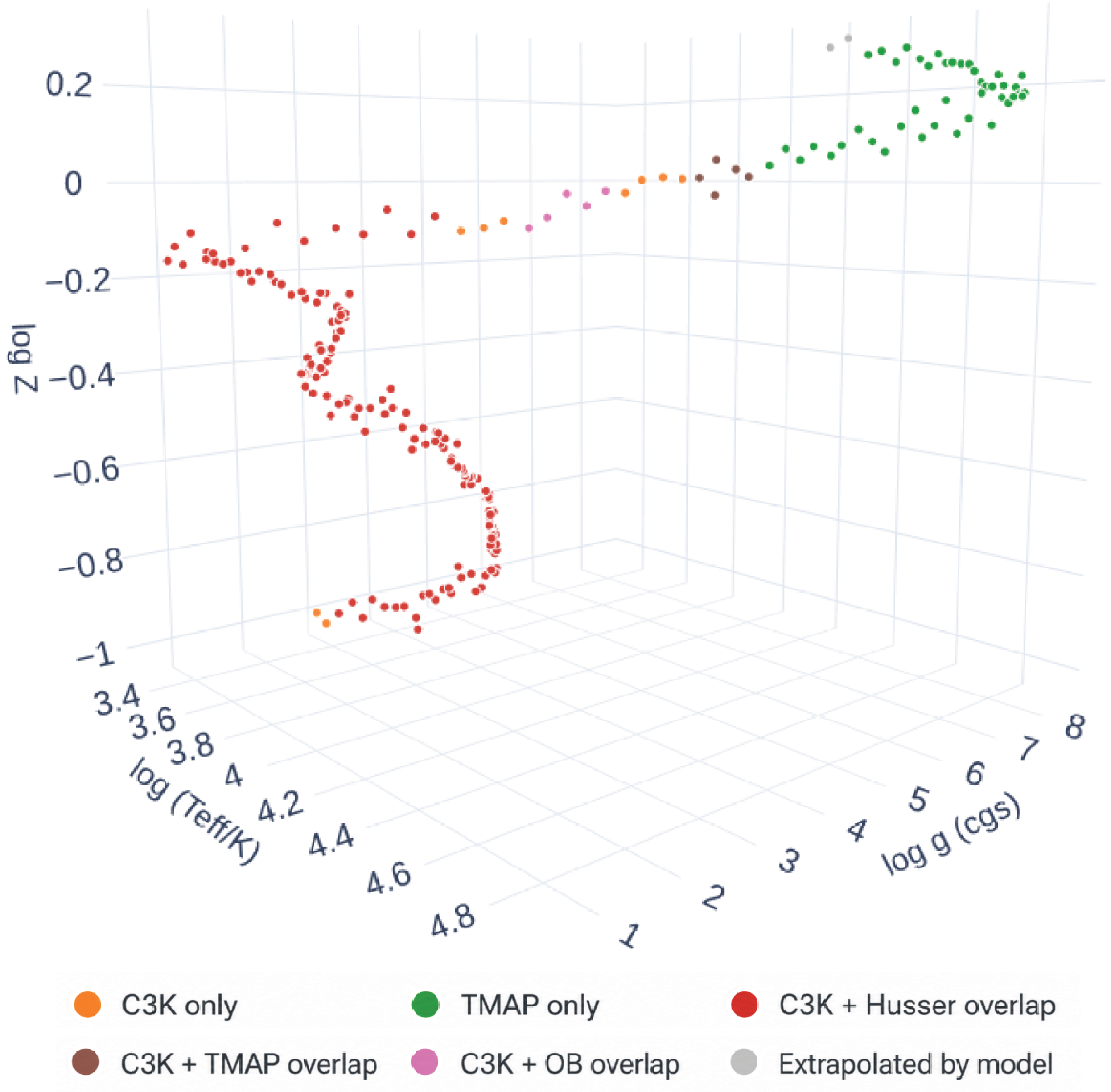
The dashboard can also be deployed on shared institutional compute resources and accessed through a web browser by multiple users within the same network. This provides a centrally managed and reproducible environment for collaborative use, without requiring separate installation on individual machines. Collectively, this GitHub-based release provides a practical, research-grade pathway for community experimentation and rapid hypothesis testing without requiring a centrally hosted web service.
8. Discussion
SM-Net provides an accurate and computationally efficient framework for generating stellar spectra. Across the combined PHOENIX–Husser, C3K–Conroy, OB–PoWR, and TMAP–Werner libraries, it achieves mean RMS flux deviations of
 $0.32\%$
,
 $0.50\%$
, and
 $0.44\%$
on the training, validation, and test sets, respectively, in the normalised log1p-scaled flux representation. It also performs robust interpolation at parameter combinations not encountered during training. Inference is performed in a single forward pass. On a single NVIDIA RTX 4090 GPU, the model achieves a throughput of approximately 14 000 spectra per second under high-throughput settings. This makes SM-Net well suited to applications requiring dense sampling of stellar parameter space, rapid spectral generation, or interactive exploration of the learned manifold.
The synthetic broad-band colour analysis complements the pixel-level reconstruction metrics by testing quantities directly relevant to photometric and stellar-population applications. The small signed colour offsets indicate that SM-Net does not introduce a substantial systematic displacement in optical–near-infrared colour space, although its typical colour differences are broader than those between the matched PHOENIX–Husser and C3K spectra. The reduced optical upper tails, together with the
 $J-K_s$
90th-percentile difference remaining below the adopted observational colour floor, show that the learned manifold broadly preserves integrated spectral-energy-distribution trends while retaining limitations inherited from the source libraries.
The line-strength analysis provides a complementary test of narrower spectral features. SM-Net closely reproduces several commonly used indices across the full test set, although CN1 shows greater scatter and H
 $\beta$
reconstruction is more challenging in parts of the OB–PoWR regime. These differences are consistent with the library-dependent spectral complexity and irregularities discussed above.
A key feature emerging from the learned manifold is the model’s ability to infer structure in masked or zero-valued flux regions. Because SM-Net treats masked values as unknown rather than physically meaningful zeros, it reconstructs missing spectral information using correlations learned across neighbouring
 $(T_{\mathrm{eff}}, \log g, \log Z)$
points. The examples presented in Section 6 demonstrate that the network draws on the smoothness of spectral morphology in local regions of parameter space, allowing it to interpolate through gaps created by incomplete line lists or numerical artefacts in the original libraries. This behaviour is physically intuitive: neighbouring points in stellar parameter space share similar continuum shapes, ionisation balances, and line strengths, and the network leverages these relationships to fill in missing structure in a manner that is often inaccessible to standard grid interpolation.
An important distinction should be made between SM-Net’s ability to interpolate within the joint parameter space spanned by the training libraries and its ability to extrapolate beyond that space. Interpolation performance is directly validated against reference spectra and constitutes the primary result of this work. Extrapolation, while supported by the continuity of the learned manifold, is not constrained by ground-truth data and should therefore be treated as exploratory. This behaviour is a natural consequence of learning a smooth functional mapping and does not imply physical correctness outside the domain sampled by the input libraries.
Despite its strengths, the present version of SM-Net also inherits several limitations from the training data and model design. First, the emulator predicts static spectra without velocity broadening or instrumental convolution. These effects must be applied downstream, analogous to the workflow used in stellar population synthesis codes. Second, the model learns the assumptions embedded in each training library, including differences in opacities and line lists across grid overlaps. Residual structure at the boundaries between PHOENIX–Husser and C3K, for example, reflects genuine inconsistencies between the physical models rather than network failure. Third, the wavelength range is constrained to the adopted 3 000–100 000 Å grid; behaviour outside this interval requires the inclusion of training spectra covering additional wavelength ranges with physical consistencies.
A critical limitation arises in the high-temperature regime (
 $T_{\mathrm{eff}} \gt 15\,000\,$
K), which is dominated by the OB–PoWR and TMAP libraries. Because these training grids do not strictly parametrise metallicity, SM-Net produces spectra that are mostly invariant to
 $\log Z$
in these regions. Users should treat this as a regime where metallicity is unconstrained by the underlying physical models. The model effectively marginalises over metallicity for hot stars; therefore, SM-Net should not be used to infer metallicities or study metallicity-dependent features (such as wind lines or line blanketing) for O-type, B-type, or White Dwarf stars. In these regimes, the
 $\log Z$
input acts merely as a dummy variable required for the network’s architectural consistency and does not represent a physical prediction of metallicity effects.
These considerations highlight opportunities for hybrid approaches combining machine-learning emulation with physical radiative-transfer modules. For example, an ML component could provide rapid coarse predictions or act as a differentiable prior, while a physics-based solver refines selected wavelength regions or enforces specific constraints (e.g. ionisation equilibrium). Such hybrid models would retain physical interpretability while leveraging the efficiency and smooth interpolation capabilities of data-driven emulators. SM-Net therefore represents both a proof of concept and a foundation for next-generation spectral synthesis frameworks that balance physical rigour with computational scalability.
9. Conclusion and future work
SM-Net provides a data-driven framework for representing the composite stellar-library dataset as a smooth and easily navigable mapping in parameter space. Rather than replacing existing libraries or physical modelling pipelines, it acts as an integration layer over the constructed training manifold, mitigating the practical effects of irregular grid sampling and enabling efficient spectral generation across the combined parameter domain. This supports analysis modes that are cumbersome with discrete template grids, including dense parameter sweeps, interactive exploration of stellar parameter space, and rapid generation of stellar spectra for downstream modelling. Validation using synthetic broad-band colours and line-strength indices further shows that this spectral accuracy generally carries through to derived observables relevant to downstream applications.
A key practical strength of SM-Net is its accessibility and the release of the code, trained weights, inference metadata, and dashboard required to use the model. The browser-based Dash demonstrator lowers the software barrier by allowing researchers to interrogate the learned manifold and generate spectra without writing bespoke interpolation or inference code. It can be run locally on compatible hardware or deployed on shared institutional computing resources.
Looking ahead, the most natural extensions of this work lie in stellar population synthesis rather than in individual stellar atmosphere libraries. A closely related manifold-learning approach could be applied directly in simple stellar population (SSP) space by generating large ensembles of population models with controlled variations in ingredients such as the initial mass function, isochrones, or underlying stellar libraries. Learning a continuous representation in this higher-level parameter space would enable efficient exploration of population-scale dependencies while maintaining a clear separation between stellar-atmosphere physics and population-synthesis assumptions.
It is also important to place SM-Net in the context of existing interpolation-based approaches. Classical schemes, such as the MSG interpolator (Townsend & Lopez Reference Townsend and Lopez2023) and the methods described in the ProGeny-I framework, provide physically motivated interpolation within discrete grids and form a valuable baseline for stellar spectral modelling. SM-Net offers a complementary alternative that is optimised for scalability, smoothness across heterogeneous libraries, and rapid inference, particularly in regimes where grid irregularities or library boundaries limit the effectiveness of traditional interpolators.
Beyond stellar atmospheres, the same manifold-learning framework could be extended to other forward-modelling tasks, including nebular emission models, binary-evolution tracks, or machine-learning-accelerated components of radiative-transfer workflows. The model could also be coupled to simple physical transformations, such as velocity broadening or instrumental response functions, to enable more direct integration with observational analysis pipelines.
In summary, SM-Net provides a flexible and efficient foundation for next-generation spectral modelling. By unifying heterogeneous stellar libraries into a coherent continuous manifold, it bridges detailed stellar atmosphere calculations and scalable analysis workflows, supporting both traditional population-synthesis applications and new, interactive approaches to exploring stellar parameter space. Its extensibility positions it well for integration into future hybrid physical–machine-learning pipelines and for meeting the demands of large-scale spectroscopic surveys in the coming decade.
Acknowledgements
We would like to extend our sincere thanks to the ProGeny team for generously sharing the libraries used for training, testing and validating the model. Luca Cortese acknowledges support from the Australian Research Council Discovery Project funding scheme (DP210100337). Aaron Robotham acknowledges support from the Australian Research Council Future Fellowship (FT200100375).
Data availability statement
The code associated with this work, including the SM-Net model implementation and the interactive dashboard, is publicly available at: https://github.com/ICRAR/SM_Net. The trained model weights are available through Zenodo at DOI: https://doi.org/10.5281/zenodo.21406957.
The stellar libraries used for training, validation and testing were provided by the ProGeny team in their processed format. These libraries are based on the PHOENIX–Husser, C3K–Conroy, OB–PoWR and TMAP–Werner stellar atmosphere grids, and remain subject to the availability, citation and licensing conditions of their respective source projects.
Appendix A. H
$\boldsymbol{\beta}$
line-strength diagnostics

To examine the origin of the negative H
 $\beta$
indices and the library-dependent reconstruction behaviour, we inspected the test spectra and fitted pseudo-continua for selected test cases.
Most negative reference H
 $\beta$
case from each input library. The reference and SM-Net spectra are shown together with the blue and red pseudo-continuum passbands, the H
 $\beta$
feature band, and the corresponding fitted pseudo-continua. The strongly negative PHOENIX–Husser and C3K indices arise where much of the feature-band flux lies above the fitted pseudo-continuum.
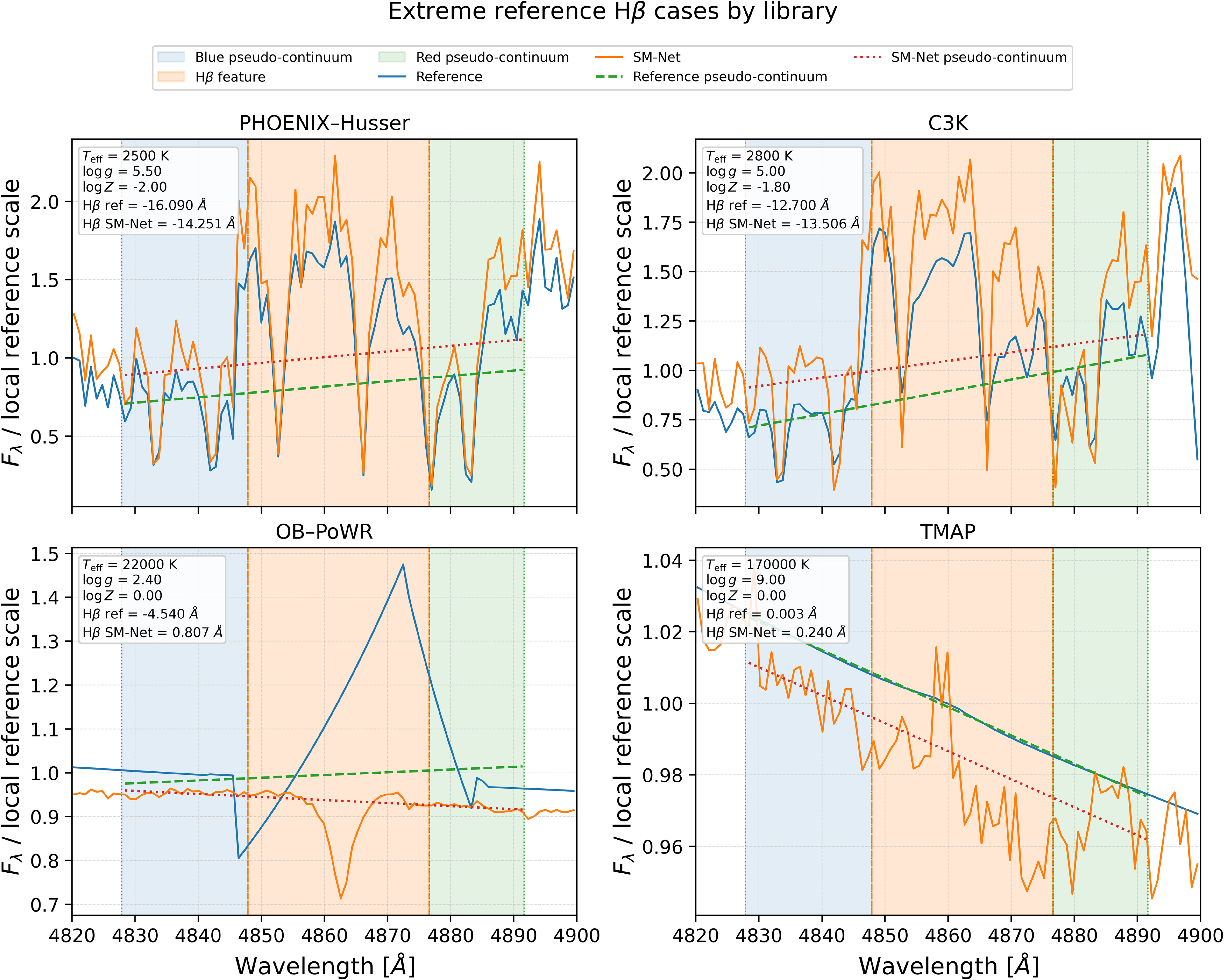
Figure A1. Long description
Panel A: Line graph for PHOENIX-Husser. The x-axis is labeled Wavelength (Å) ranging from 4820 to 4900. The y-axis is labeled Fλ / local reference scale ranging from 0.5 to 2.0. The graph shows blue pseudo-continuum, red pseudo-continuum, Hβ feature, reference, and SM-Net spectra. Panel B: Line graph for C3K. The x-axis is labeled Wavelength (Å) ranging from 4820 to 4900. The y-axis is labeled Fλ / local reference scale ranging from 0.5 to 2.0. The graph shows blue pseudo-continuum, red pseudo-continuum, Hβ feature, reference, and SM-Net spectra. Panel C: Line graph for OB–PoWR. The x-axis is labeled Wavelength (Å) ranging from 4820 to 4900. The y-axis is labeled Fλ / local reference scale ranging from 0.7 to 1.5. The graph shows blue pseudo-continuum, red pseudo-continuum, Hβ feature, reference, and SM-Net spectra. Panel D: Line graph for TMAP. The x-axis is labeled Wavelength (Å) ranging from 4820 to 4900. The y-axis is labeled Fλ / local reference scale ranging from 0.96 to 1.04. The graph shows blue pseudo-continuum, red pseudo-continuum, Hβ feature, reference, and SM-Net spectra.
Representative non-extreme H
 $\beta$
reconstructions from each input library. Cases were selected to have a meaningful H
 $\beta$
feature and good agreement in both the measured index and the local feature shape. The OB–PoWR example illustrates the comparatively greater difficulty of reconstructing this library.
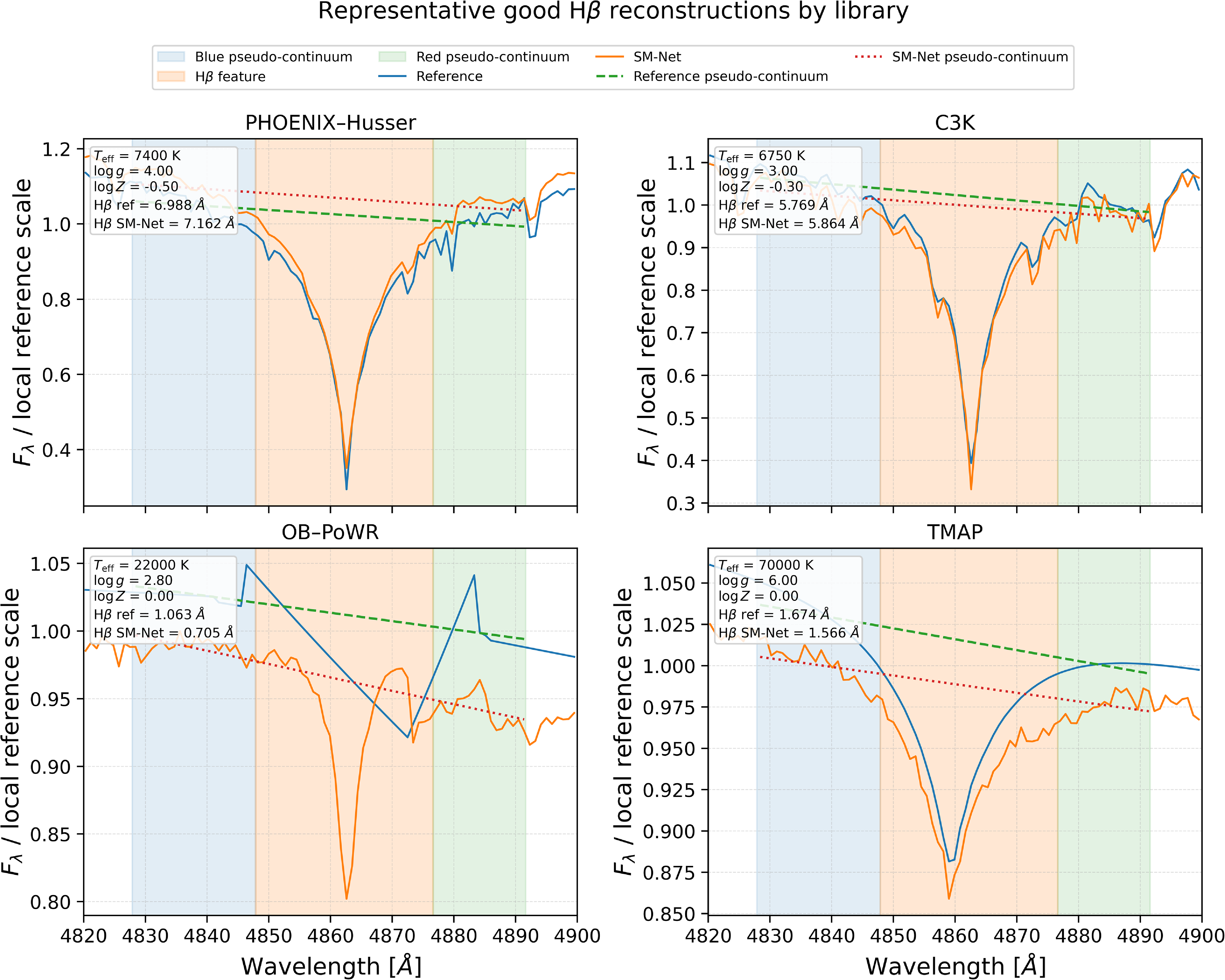
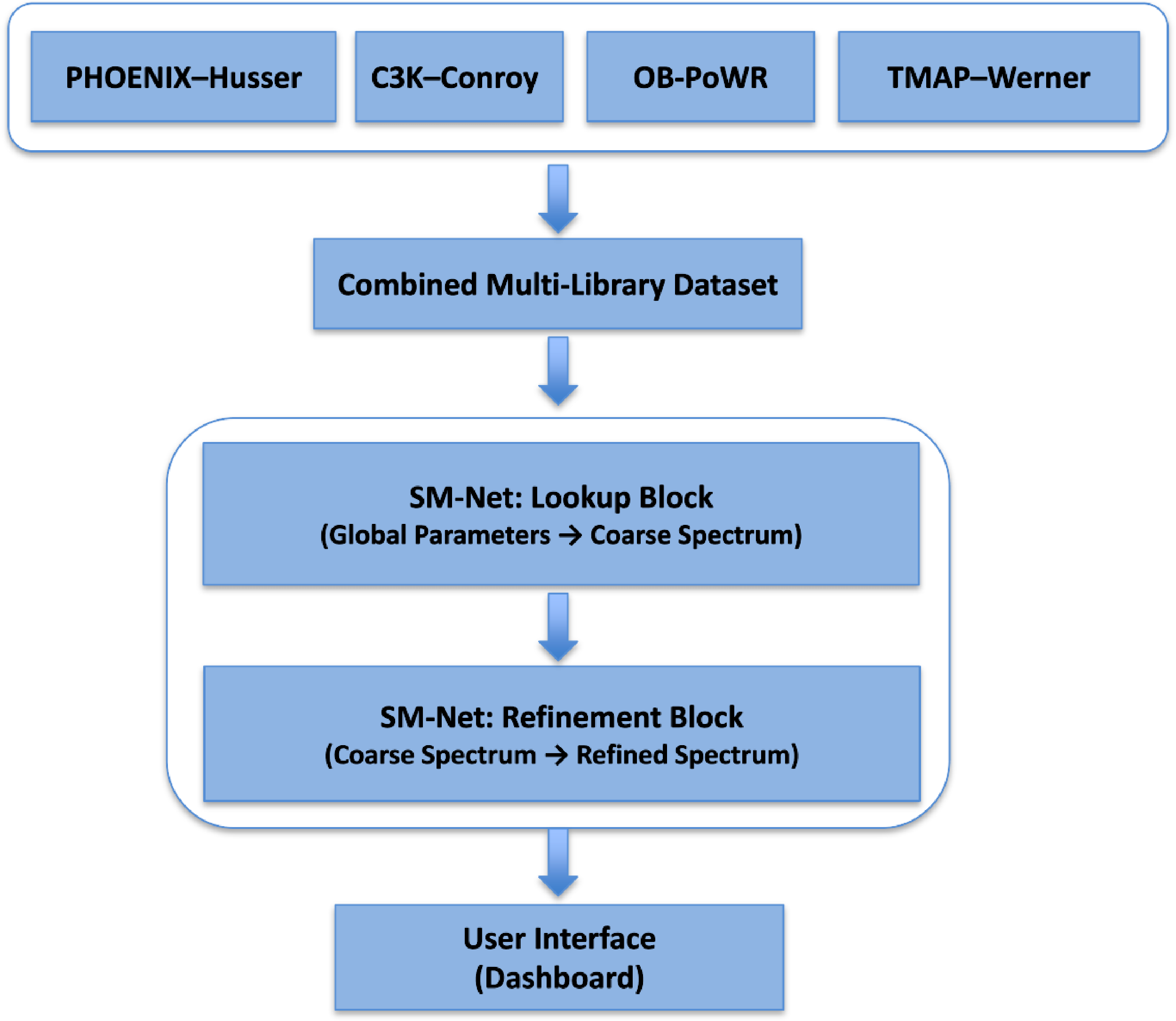

 logg≡log10[g/(cms−2)]
 logZ≡log10(Z/Z⊙)
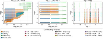
 log10(Teff/K)
 logg
 log10(Teff/K)
 logZ
 logZ
 logg
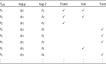
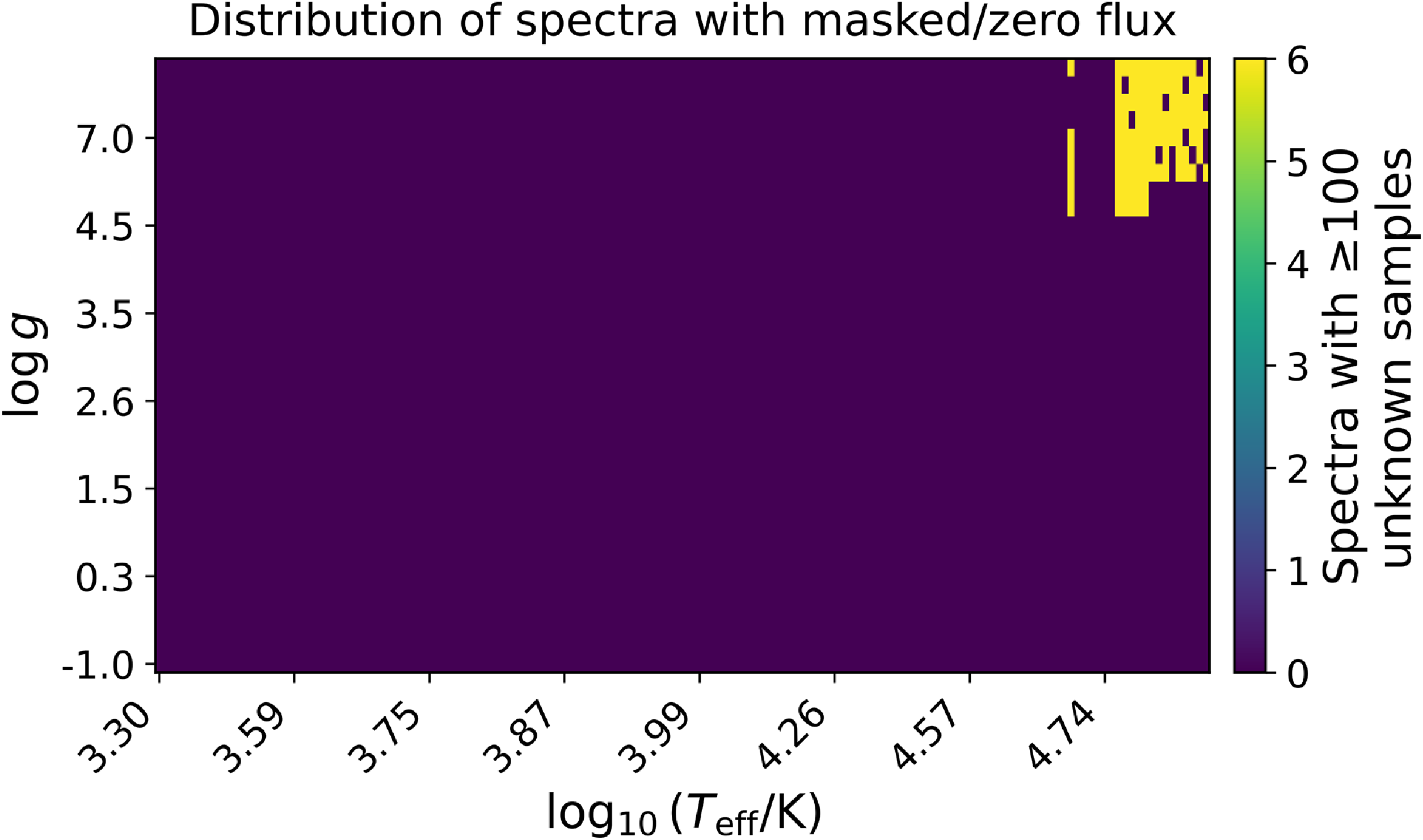
 logZ
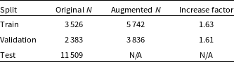
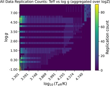
 logZ
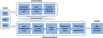
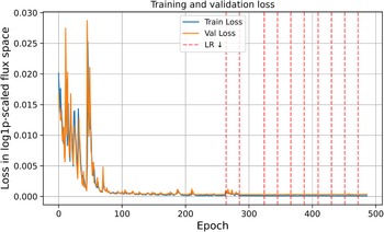
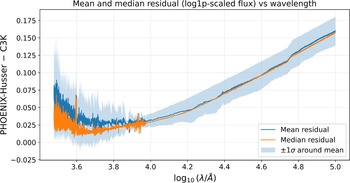
 log10(λ/
 −
 (Teff,logg,logZ)
 ±1σ
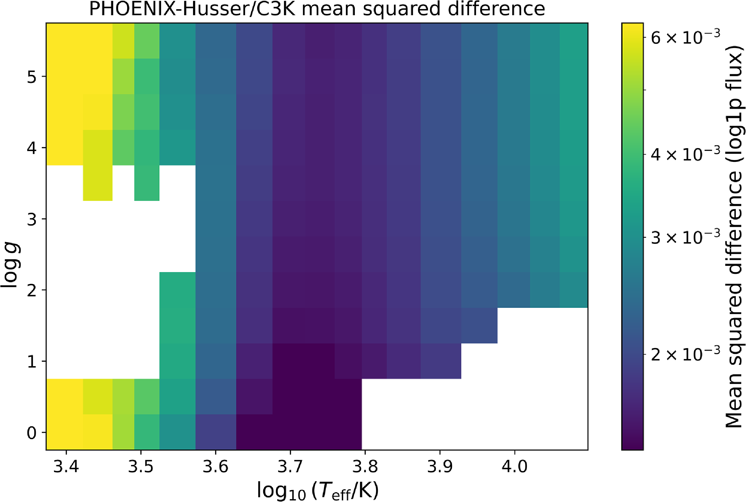
 log10(Teff/K)
 logg
 logg
 logZ
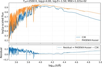
 Teff=2500K
 logg=4.0
 logZ=−1.5
 −
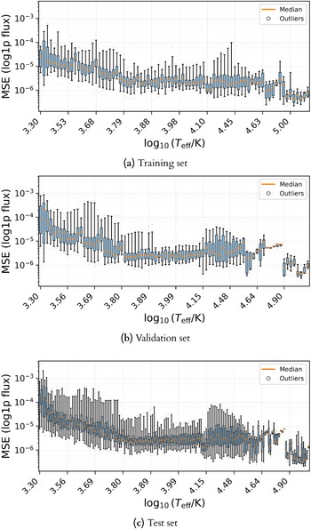
 log10(Teff/K)
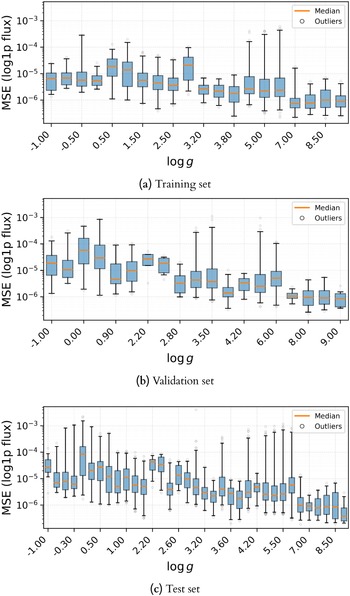
 logg
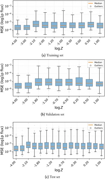
 logZ
 logZ=−4
 −3

 RMSflux
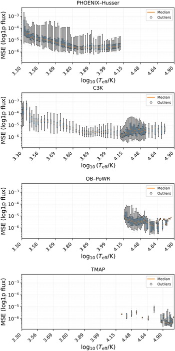
 log10(Teff/K)
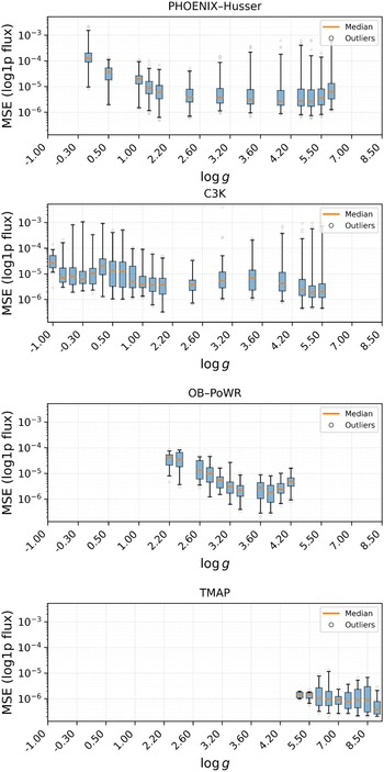
 logg
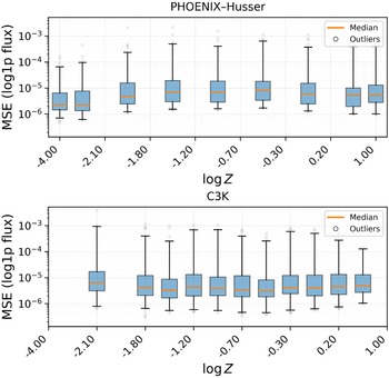
 logZ
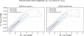
 (g−i)AB
 (J−Ks)AB
 Teff=5800
 logg=4.5
 logZ=0
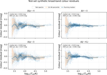
 Δ(X−Y)=(X−Y)reference−(X−Y)SM-Net
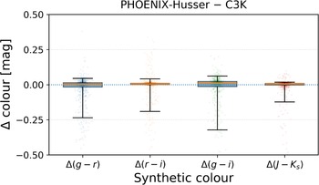
 −
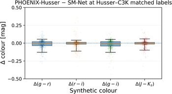
 −
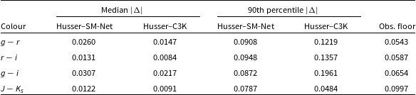
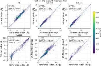
 β
 log10(Teff/K)
 R2
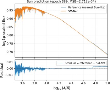
 −
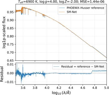
 Teff=6900K
 logg=4.0
 logZ=−2.0
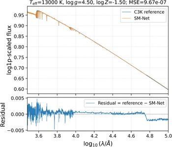
 Teff=13000K
 logg=4.5
 logZ=−1.5
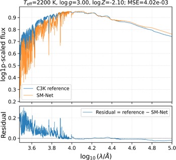
 Teff=2200K
 logg=3.0
 logZ=−2.1
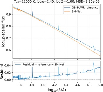
 Teff=22000K
 logg=2.4
 logZ=−1.0
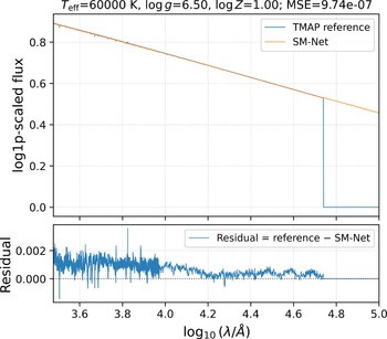
 Teff=60000K
 logg=6.5
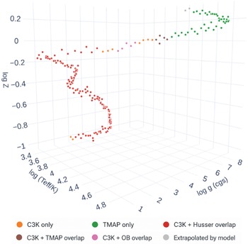
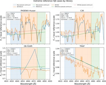
 β
 β
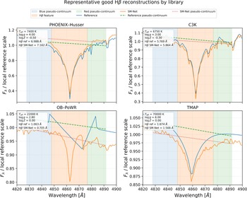
 β
 β

 Open access

