1. Introduction

Considerable research has been done on the thermohaline circulation of the Atlantic Ocean by a number of authors (Reference Bryan.Bryan, 1986; Reference Zhang, Lin and Greatbatch.Zhang and others, 1992. Reference Zhang, Greatbatch and Lin.1993, Reference Zhang, Lin and Greatbatch.1995; Reference Wright, Stocker. and PeltierWright and Stocker, 1993). However, the treatment of the sea-ice cover has been limited. Many aspects of the thermohaline circulation are largely controlled by the surface boundary conditions on salt and heat. Because of the importance of the role of these boundary conditions, we expect that sea ice may play a particularly important role in the thermohaline circulation. Specifically, the presence of au ice cover tends to insulate the ocean while the melting and freezing can modify the salt fluxes. This is especially true when ice transport is included, inasmuch as melting southward-moving sea ice can both cool the ocean and deliver a substantial fresh-water flux, This salt flux may be quite critical as most investigations have indicated that perturbations of the sali flux can lead to a catastrophic breakdown of the thermohaline circulation (see, e.g., Reference Bryan.Bryan, 1986). This feature is an important component of the effect of Heinrich events on ocean circulation (Reference Wright, Stocker. and PeltierWright and Stocker. 1993).

In addition to the salt flux, the insulating effect of sea ice can play a role in altering the thermohaline circulation, Moreover, it has been demonstrated that the presence of a thermodynamic sea-ice cover can lead to short-term oscillations of the ice–ocean system (Reference Zhang, Lin and Greatbatch.Zhang and others, 1995). However, how the dynamic character of the ice cover might affect such oscillations has not been examined. Also the precise physical mechanisms are not fully understood.

Because of these complexities, in this paper we focus on the thermodynamic effects of the sea-ice cover and the role of the sea-ice dynamics on the inter-decadal and shorter oscillatory characteristics produced by the presence of interactive sea ice. The focus in this study is on the physical mechanisms responsible for such oscillations, and the role ice dynamics play in modulating the oscillatory behavior. As a consequence an idealized mechanistic model is used here. While this model only very crudely approximates the North Atlantic, the mechanisms appear robust enough to motivate investigation with more complete circulation models.

Overall the simulations demonstrate that the inclusion of interactive sea ice intrinsically causes substantial oscillation in the thermohaline circulation and northward heat transport. That this mechanistic model result may have more general application is also consistent with more complete model-based studies of the inter-annual variability of the ice–ocean system which indicate that, with ice dynamics included, inter-annual variations of the Greenland Sea ice margin are largely controlled by a balance between oceanic heat transport and ice advection (Reference Hibler and Zhang.Hibler and Zhang, 1994).

2. Model Description

For this study, we make use of a mechanistic sector geostrophic ocean model. The model domain is bounded by latitudes 5° and 65° N (a latitude just north of Iceland) and longitudes 50° W and 10° E. The model is in spherical coordinates and has a horizontal resolution of 2.3° in both latitude and longitude, with 14 vertical levels as shown in Table 1. This ocean model is somewhat similar to that used by Zhang and others (in press), although there are differences. Specifically, for all equations of motion we utilized a flat-bottom version of the Bryan Cox ocean circulation model with the non-linear terms removed and a simplified equation of state (Zhang and others, in press), so that we essentially have a planetary geostrophic model. However, one major modification is that we have increased substantially (by a factor of five) the viscosity of the bottom layer. This effectively creates a greater damping of the external mode and also produces a bottom torque term resulting in some baroclinic adjustment in the upper layers similar to what occurs with bottom topography. As a consequence, in this model, as contrasted to other planetary geostrophic models, changes in the density field will also cause the vertically integrated flow to change; hence the vertically integrated flow must be recalculated at each time step, not once as is the ease in other geostrophic models. This is considered to be a realistic feature of the model, since to a large degree it mimics the bottom torque effects of bottom topography. Also, it provides a consistent set of equations as we simply integrate the primitive equations forward in time without the non-linear terms. In this model, the horizontal and vertical kinematic eddy viscosity are 5 × 10⁸ and 1 cm² s⁻¹, respectively, and the horizontal and vertical diffusion coefficients are 2 × 10⁷ and 0.63 cm² s⁻¹.

Table 1.

Thicknesses of ocean vertical levels

For forcing fields we have an east–west zonally invariant surface wind stress with surface air temperature and surface ocean salinity specified in a zonally uniform manner with meridional variations. The wind stress, temperature and salinity fields are essentially the same as used by Zhang and others (in press) except that we have made the temperatures slightly colder by subtracting a linearly increasing temperature increment. Consequently, our air temperatures ranged from 27.5°C at 5° N to −10.15°C at 65° N. The cross-over to below-freezing temperatures occurs at about 51° N.

For modeling sea ice, we made use of a dynamic thermodynamic sea-ice model coupled to the ocean in a manner similar to that employed by Reference Hibler and Bryan.Hibler and Bryan (1987), except that a cavitating fluid rheology (Reference Flato and Hibler.Flato and Hibler, 1992) in spherical coordinates was employed. In addition, only one level of ice was used, with only a mean ice thickness and no open water. For the dynamic sea-ice model, an additional southward surface wind stress of 10 mPa (0.1 dyne cm⁻²) was imposed. Additionally, a mean ice thickness of 2 m and a southward ice velocity of 0.02 m s⁻¹ were imposed at the northern boundary as an open boundary-flux condition. Basically, with this formulation the ice motion will be affected by the ocean currents but will not modify the oceanic momentum equations.

Since there is no seasonal cycle here, the coupling to the atmosphere was simplified, in that we parameterized the heat flux as what would occur for sensible heat fluxes only. In the case of open water, this yields a heat flux of

(1)

where Τ _a is the air temperature and T ₁ the surface water temperature. The bulk transfer coefficient D has been chosen to yield fluxes equivalent to having a 30d relaxation in the ocean-conservation equations for temperature. This value is slightly higher than that of Reference Hibler and Bryan.Hibler and Bryan (1987), but is being used in a mean annual context. In the case of an ice cover we assume a constant conductivity k through the ice and no heat storage. With this assumption, together with insisting that the heat flux is continuous, it is easy to show that the air–sea heat exchange in the presence of sea ice of thickness h is given by (see. e.g., Reference Hibler, Flato. and TrenberthHibler and Flato, 1992)

(2)

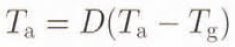
where

(3)

and where T _f is the freezing temperature of sea water. Consistent with Reference Hibler and Bryan.Hibler and Bryan (1987), the melting effects of the ocean on the ice are obtained by insisting that the upper layer of the ocean is at freezing in the presence of ice. To accomplish this, sufficient ice melt to lower the ocean to freezing takes place at the end of each time step.

For the surface salt flux we used a 30 d relaxation to mean meridional values in the ocean salt-conservation equations. For all the model simulations discussed here, the relaxation terms for both salt and heat exchange were always employed.

In addition to these ice models, we also performed two “fixed ice-thickness” control simulations. In the first, or “zero ice-thickness” case, the insulating effect of the ice is removed by simply insisting that whenever the freezing point of sea water is reached by the ocean, the ocean temperature is not allowed to drop any lower. However, no ice is allowed to form. This effectively removes the insulating effect of sea ice. In the second control simulation, a fixed ice cover is specified, and heat transfer into the ocean is calculated using Equation (3) except that T _f is taken to be the temperature of the water underneath the ice which may be above freezing. As in the “zero ice-thickness” case, the ocean surface temperature is constrained only by not being allowed to drop below freezing and is, in fact, allowed to go above freezing under the ice. Consequently, in this simulation the insulating effect of the ice cover is treated even though there is no interaction between the ice and the ocean.

3. Model Simulations

Using the numerical model described above, four model simulations to a quasi-equilibrium obtained aller about 5000 years of model integration were carried out. In all cases, the ice–ocean model was initialized with uniform temperature and salinity. The three simulations that were performed used the different ice formulations mentioned above, namely a motionless simulation where a motionless thermodynamic ice model was employed; an “ice-dynamics simulation” where ice transport and ice dynamics employing a cavitating fluid rheology were employed; a control “zero-ice” run where no ice was allowed but the ocean was not allowed to drop below the freezing temperature; and a “fixed-ice simulation” where the insulating effects of the ice cover were imposed but no other interaction was allowed.

3.1 Approach to equilibrium

Each model was integrated at 1 d time steps for about 5000 years. The long-term total ocean energies and total ocean temperatures are shown in Figure 1. Basically, after an intermediate oscillation, the models approach an equilibrium state with relatively stable results. This is also true of the ice extent and thickness for the two models including sea ice (Fig. 2). Note that the temperature is coldest with the zero-thickness ice run and warmest with the “fixed-ice” control model. This is consistent with the heat transfer at high latitudes being highest in the zero-thickness case and lower with sea ice present. Moreover, in the “fixed-ice” model, there is no cooling of the ocean by melting sea ice. Note that the ice-dynamics case is only slightly warmer than the motionless interactive-ice case. This is because even though, as shown in Figure 3, the ice cover is consistently thicker for the ice-dynamics model, the ocean is also cooled by melting southward-moving sea ice. The thermohaline circulation pattern is very similar in the interactive sea-ice cases and is shown in Figure 4 where the meridional-stream functions for the “ice-dynamics” and “zero-ice” simulations are shown. Note that in the ease of the “zero ice-thickness” model, the excessive cooling at high latitudes moves the dominant sinking to a slightly higher latitude but shuts off the very high-latitude circulation. In the “fixed-ice” simulation there is a more subtle enhanced high-latitude cooling. This cooling follows from a warmer high-latitude temperature arising from not forcing the ocean temperature to freezing by melting sea ice. It is felt that part of the reason that such large overturning occurs farther south in these simulations is the somewhat excessively cold temperatures used here at high latitudes.

Fig. 1.

Averaged ocean temperature over the whole model domain (°C) and total kinetic energy (cm² s⁻²) for the motionless interactive sea-ice model (solid line), the ice-dynamics model (dotted line), the control run with zero ice thickness (dashed line) and the control run with fixed ice thickness (dot-dashed line).

Fig. 2.

Mean ice coverage (fraction of whole ocean surface area) and ice thickness (m) averaged over the region covered by ice. The solid line is for the motionless interactive ice model and the dotted line for the full ice-dynamics model. For comparison, the fixed-ice control ran has a mean ice thickness of 1 m and menu ice extent of 0.154.

Fig. 3.

Ice thickness distribution for (a) the motionless interactive-ice model and (b) the ice-dynamics model. Contour interval is 0.1 m. For comparison the fixed-ice simulation has 1.0 m thick ice extending down to 55.8° N.

Fig. 4.

Overturning stream-function contours for (a) the ice-dynamics model and (b) the control simulation with Zero ice thickness. The motionless interactive sea-ice model yields stream-function contours very similar to those for the ice-dynamics model while the fixed-ice thickness model has a stream function intermediate between (a) and (b). Contour interval is 1 Sv.

These circulation patterns are also reflected in the northward heat transport for the four models shown in Figure 5. In the two models including interactive sea ice,the northward heat transport peaks at around 18° N and then gradually declines, although there is significant northward transport at high latitudes. In the zero ice-thickness case, there is a higher transport below about 30° N and then a substantial reduction of transport farther north.

Fig. 5.

Northward heat transport (10¹² cm² °C s⁻¹) vs latitude for the ice-dynamics model (solid line), the zero-ice control simulation (dotted line) and the fixed-ice control model (dashed line). The heat transport for the motionless interactive sea-ice model is indistinguishable at this scale from that for the ice-dynamics model.

3.2 Oscillatory characteristics

Of particular interest for this paper are the oscillatory characteristics of the “steady-state” version of the two models including interactive sea ice. Many characteristics of these oscillations can be explained by some simple idealized model concepts presented later. In Figure 6 are shown 100 year long amplified time series of the ice coverage and ice thickness for the two models including interactive sea ice. To compare the ocean temperature characteristics, Figure 7 shows time series of the same 100 years of ocean temperatures north of 46.6° N (averaged over the upper 531 m of the ocean) and surface heat fluxes for the same region. Finally, selected ocean circulation characteristics are illustrated in Figure 8, which shows the northward volume transport at the middle of the ocean grid in the upper 531 m of the ocean and the northward ocean heat transport at 46.6° N. Reported in the figure captions are the steady-state values for these oceanic variables for the control simulations, demonstrating the stability of the control simulations.

Fig. 6.

Mean ice coverage (fraction of whole ocean surface area) and ice thickness (m) averaged over the region covered by ice at “steady state”. (a1, a2) The motionless interactive ice model; (b1, b2) the ice-dynamics model.

Fig. 7.

Mean water temperature (°C) and surface heat fluxes (W m⁻²) for the region north of 46.6° N. The water temperature is for the upper 531 m of the ocean. (a1, a2) The motionless-ice model; (b1, b2) the ice-dynamics model. For comparison, the control simulations (zero ice and fixed ice, respectively) have temperature variations of 3.3838–3.3840°C and 5.9614–5.9622°C; and heat-flux variations of −247.918 to −247.917 W m⁻² and −51.54 to −51.44 W m⁻².

Fig. 8.

Mean water transport variations (Sv) in the upper 531 m of the ocean at the center of model domain and heat transport ( 10¹²cm² °C s⁻¹) at 46.6° N for (a1, a2) the motionless-ice model and (b1, b2) the ice-dynamics model. For comparison, the transports for the control runs (zero ice and fixed ice) are 5.5004–5.5012 and 4.4389–4.4408 for water transport, and 10.3717–10.3723 and 38.161–38.173 for heat transport.

It is very clear from Figures 6–8 that the inclusion of thermally interactive sea ice causes the models to have significant oscillatory characteristics. Since the only boundary condition that is directly changing because of the ice is the heat transport into the ocean, the effect that is being illustrated here is that the insulating characteristics of sea ice are leading to oscillations in the thermohaline circulation when the ocean is allowed to melt back the ice.

It is also clear that the main role of ice dynamics and transport is to decrease the amplitude of the oscillations and somewhat alter the phase of the highest frequency.

This is shown perhaps more graphically in Figure 9 where we show power spectra of the different time series. The dominant oscillatory characteristic is a high-frequency fluctuation with a period of around 5 years in the ice and temperature variables at high latitudes. These high-frequency fluctuations are also present in the actual heat transport and to a lesser degree in the upper-ocean volume transport (Fig. 8).

Fig. 9.

Power spectra of time series. Solid lines are from the ice-dynamics model and dashed lines are from the motionless-ice model.

In the case of the water transport (especially in the simulation including sea-ice dynamics), there is also a longer-term quasi-periodic variability with a period of about 20 years. These oscillations are either not present in the control simulations or at least an order of magnitude smaller. The overall magnitude of the oscillation in the oceanic-water and heat transport is about 2% for the motionless-ice case and about 1% for the ice-dynamics model. The surface temperature variations (relative to 0°C) have similar percentage changes, while the heat-flux variations are very substantial (23% and 8% for the motionless and ice-dynamics models, respectively). These larger variations reflect the substantial variability in the ice thickness of about 40% and 10% for the two models.

It is also useful to note that, while in all cases the dynamic-ice model yields small oscillations, it is in the percentage change in ice thickness that the biggest difference occurs. In particular, the ice thickness in the ice-dynamics model has a maximum oscillatory change of about 0.04 m which is only slightly smaller than the thermodynamics-only case of 0.06 m. Also, both models have very similar ice extents, with relatively small changes of about 11% and 6%, respectively, for the motionless and ice-dynamics cases.

4. Discussion and Conceptual Model

The dominant result shown by this numerical model is that inclusion of an ice cover (Which directly affects only the sea–air heat fluxes and not the salinity fluxes) results in pronounced short-term oscillations of ice extent, ice thickness, ocean temperature, transport and energy. In the case of sea-ice thickness, extent and surface heat exchange, these oscillations are substantial (~10%), but they form a much smaller percentage in the case of the ocean volume and heat transports (~1%). The main effects of the inclusion of ice transport and dynamics are that the magnitude of the oscillations is reduced and the dominant high-frequency component is shifted from a 5 year period to a higher frequency of about 4 years. Also, in terms of specific variables, the ice-extent variations are cut in half when dynamics is included, while the thickness variations are similar in magnitude. However, because of greater ice mass in the ice-dynamics case (resulting from ice being transported southward), the percentage change in thickness is much less.

In terms of a conceptual model, the high-frequency oscillatory characteristics can be qualitatively explained by considering an ice cover on top of a warm ocean which is receiving heat laterally. As the ocean warms, it melts the ice and is then cooled by the sea–air heat transfer. Basically we can imagine starting off with a cold ocean and a thin ice cover. Under these circumstances the ice then thickens rapidly. However, as the ice becomes thicker, it insulates the ocean more effectively. As tins occurs, the ocean warms up and eventually melts the ice back, which then allows the atmosphere to cool the ocean, and the cycle starts over again.

However, this simple view is complicated by the fact that the lateral heat transport also changes in response to changes in the ocean temperature. The interaction and phase relationships between these variables are shown more clearly in Figure 10, which compares 40 year time series of the ocean temperature of the upper 531 m of the ocean north of 46.6° N, and the heat transport. In Figure 11, the cross-correlation between these variables is plotted to establish phase differences better. These figures show that the ice thickness and ocean temperature are out of phase as we would expect. Moreover, examination of the time series shows (especially in the motionless sea-ice cover case) that there is a very sharp drop in the ocean temperature coincident with a very sharp peak in the northward heat transport. What appears to be happening here is that a strong cooling at the surface when the ice is very thin results in a surge in northward heat transport (not necessarily at the surface). Once this dies down, the ice thickens again and the ocean gradually warms up.

Fig. 10.

40 year time series of ice thickness, water temperature and heat transport across 40.6° N. The variables were averaged over the regions as described in Figures 6–8.

Fig. 11.

Cross-correlation between mean ice thickness and wean temperature (solid line), ice thickness and heat transport (dotted line), and heat transport and ocean temperature (dashed line). The lag arrangement is such that at τ = −2 the correlation is for the first variable at time t with the second variable 2 years earlier. See Figures 6–8 for a description of the variables.

The longer-term cyclical effect can be related to the northward oceanic transport in the thermohaline system. Basically we can imagine that the rate of change of the northward oceanic transport would roughly scale with the rate of change of the ice thickness. Ibis assertion is reasonable in the sense that a bigger change in ice thickness corresponds to a larger cooling and, since we expect the strength of the northward transport to scale with the cooling, increased cooling will correspond to an increased northward transport.

A final issue is the fact that the model including ice dynamics has a higher-frequency oscillation than the model with motionless sea ice. The qualitative argument here is that the coupling between the rate of ice-thickness decrease and ocean-water temperature is stronger for the model with ice transport included. The idea is that with a dynamic ice cover the thickness is being controlled mainly by the southward transport of ice. Hence, in this case, warmer water directly melts a certain amount of ice without significantly changing the thickness. In the motionless-ice case, on the other hand, the thickness is dictated by a balance between ice growth and melting by the ocean. Hence there is a negative feed-back, since as the ice is melted by the water it will become thinner and grow somewhat faster. With this negative feed-back, the rate of change of ice thickness should scale less strongly with water temperature. This argument is consistent with the time series in Figures 6 and 7 where the mean ocean temperature-oscillation change is halved with the inclusion of dynamics while the thickness changes are similar. These qualitative concepts may be put in equation form as follows. For the ice growth we have

(4)

where h is some kind of average ice thickness, T _g is the surface temperature of the ice, T _w is some kind of water temperature, and T _f is the freezing temperature of sea water, The first term of this equation is the heat transfer through the ice and the second term is some type of idealized melting term. For the rate of change of water temperature we have

(5)

where, as before, h is some kind of average ice thickness and T _tr is the northward oceanic heat transport. Finally, for the northward oceanic heat transport T _tr we argue that

(6)

If we now argue that the rate of transport embodied in Equation (6) occurs at a lower frequency than the rate of change of ice thickness, we can differentiate Equation (5), and combine it with Equations (4) and (6), and separate out the two different frequency components (as the equations are essentially linear), obtaining

(7)

for the high frequency and

(8)

for the lower frequency. Both equations are oscillation equations.

The argument that there is a weaker coupling at the high frequency for the motionless-ice model is also borne out by examining the relative magnitudes of the thickness and temperature variations shown in Figure 10. Specifically, for the motionless model, the ratio of the thickness variance to the temperature variance is less than that for the simulation including ice dynamics.

In practice, of course, the two oscillations are not perfectly decoupled, and there is likely quite a lot of auto-regressive behavior that places these peaks in a red-noise background. As a consequence, this simple model should be considered qualitative. However, it is useful to get some structure to help explain some of the main characteristics of the oscillatory behavior of these two simulations.

5. Concluding Remarks

The main result of this paper is that inclusion of the insulating effects of sea ice in a hemispheric ice–ocean model naturally induces oscillations in the ocean temperature and ice thickness as well as in the thermohaline circulation when the ocean is allowed to melt back the ice. While not extremely large (4% for the ice margin and 10% for the thickness), the magnitude of the oscillations is commensurate with inter-annual variations in the Greenland Sea ice margin (see, e.g., Reference Hibler and Zhang.Hibler and Zhang, 1994). These oscillations do not depend on direct modification of the salt fluxes by ice inciting and freezing but are strictly due to the insulating effects of the ice combined with the melting effects of warmer water. The oscillatory characteristics can be explained by considering a thickening ice cover to lead concurrently to warming of the ocean by either reducing the sea–air heat loss and/or increasing the northward heat transport in the thermohaline circulation. As the ocean warms up, it eventually causes the ice to stop thickening and start thinning, which in turn will cool the ocean. At the point at which the ocean then becomes cool, the cycle starts over again.

With the inclusion of ice dynamics, the oscillations still occur bin are somewhat decreased in magnitude. Also, the southward transport of ice creates a much thicker ice cover with an extent slightly farther south. The reduction of magnitude of the oscillations can be qualitatively argued to be due to a thicker and more stable ice cover more controlled by the southward ice transport, and hence more fixed in space, than in the thermodynamic-only case.

One important difference relevant to real oscillations in the climate system is that with dynamics included, although the ice thickness changes significantly (10%) during the oscillation, the ice margin changes less (about 4%). This result in turn suggests that if such an oscillation is present in the North Atlantic it would be quite hard to see in the ice-margin record, even though it might be occurring in the thickness of the ice cover in the marginal seas. This would be especially so in light of seasonal and inter-annual simulations of the ice margin by Reference Hibler and Zhang.Hibler and Zhang (1994) which suggest that inter-annual variations of the Greenland Sea ice margin are largely controlled by fluctuations in the ice-mass transports out of the Fram Strait.

A particularly interesting feature of the low-frequency oscillations in this model is that they are close to the same frequency range as dominant δ(O¹⁸/O¹⁶) oscillations observed in Greenland ice-core records (Reference Hibler and Johnsen.Hibler and Johnsen, 1979) and in North American temperature records (Reference Mock and Hibler.Mock and Hibler, 1978). Specifically, Hibler and Johnsen (1979) found that a dominant feature of the isotopic ratios in the Greenland Dye 3, Crête and Milcent ice cores over the last 800 years was an oscillation with about a 29 year period. There were also higher-frequency peaks at around 3–7 years observed in the spectra. This “20” year oscillation was also the dominant oscillation found in shorter-term North American temperature records by Mock and Hibler (l978), especially in the northeastern U.S.A. These similarities between temperature-record variations and the oscillations produced in this simple geostrophic ice–ocean model provide motivation to investigate possible coupling effects in the ice–ocean system in more detail.

It should be emphasized that the results reported here have been obtained with an idealized sector ice–ocean model without seasonal forcing and with a number of aspects of the coupling (most notably salt fluxes by melting and freezing ice) neglected. As a consequence, while they are qualitatively quite useful, the degree to which such oscillations may be present in more physically complete ice–ocean circulation models is not clear. However, because we feel certain key variables and major processes are included, these mechanistic model results are significantly thought-provoking, a goal which has been the main thrust of this paper. Clearly what is needed is more complete analyses using more realistic models of the Atlantic and Arctic including seasonal variability.