





1. Introduction
The historical and instrumental records of major earthquakes are generally too short to provide reliable statistics for evaluating seismic risk. Alternatively, the records can be extended using sediment deposits from past earthquakes, but this requires distinguishing earthquake-triggered deposits from those formed by other causes (e.g. storm surges) (see e.g. Pouderoux et al. Reference Pouderoux, Lamarche and Proust2012; Strasser et al. Reference Strasser2024; Seibert et al. Reference Seibert2024a
). Several methods have been proposed to achieve this goal (Goldfinger Reference Goldfinger2011). Over the last decade, paleoseismology studies have focused on extracting more specific earthquake information, such as earthquake types (megathrust, intraslab or crustal) or magnitudes, from the deposits (Moernaut et al. Reference Moernaut2017; Van Daele et al. Reference Van Daele, Araya-Cornejo, Pille, Vanneste, Moernaut, Schmidt, Kempf, Meyer and Cisternas2019; McHugh et al. Reference McHugh, Seeber, Rasbury, Strasser, Kioka, Kanamatsu, Ikehara and Usami2020; Howarth et al. Reference Howarth2021). Recently, a new mechanism of direct co-seismic sediment remobilisation has been identified: surficial sediment entrainment induced by the movement of the seafloor relative to ambient water. This motion spans a wide range of time scales, from fractions of a second to minutes. In this study, we focus on two scales: long-period displacement, which involves speeds of up to
 ${\sim} 1\, \mathrm{m\,s}^{-1}$
over periods of minutes (Seibert et al. Reference Seibert, McHugh, Paola, Seeber and Tucker2024b
), and high-frequency bed ‘shaking’ involving both vertical and horizontal components. The long-period displacement induces a quasi-steady shear stress that affects the bed similarly to an ordinary current. The high-frequency components can reach accelerations in excess of
 ${\sim} 1\, \boldsymbol{ g}$
(Seibert et al. Reference Seibert, McHugh, Paola, Seeber and Tucker2024b
); the effects of such motion on sediment transport are unknown, but basic mechanical considerations indicate that they could significantly enhance entrainment. Here,
 $\boldsymbol{ g}$
is the gravitational acceleration. This mechanism was proposed by McHugh et al. (Reference McHugh, Seeber, Rasbury, Strasser, Kioka, Kanamatsu, Ikehara and Usami2020) to explain specific deposits identified in the mid-slope terrasses and trench along the Japan subduction zone and associated with the 2011 Mw 9.0 Tohoku-Oki earthquake, which resulted in the remobilisation of a thin layer of surficial sediment over a large area. This unique and unusual mechanism could be key to interpreting sedimentary deposits and learning about extreme earthquakes, which motivated the present study on the fundamental dynamics of sediment remobilisation in flows over vibrating beds.
Recently, Seibert et al. (Reference Seibert, McHugh, Paola, Seeber and Tucker2024b
) conducted physical experiments to investigate how the combination of quasi-steady shear stress and vertical high-frequency vibration at the sediment/water interface can entrain sediment. Following the above-mentioned discussion, in the experiments, the full spectrum of seismic waves was simplified into two components: (a) quasi-steady long-period shearing (associated with S waves in an earthquake), which is represented in the experiments by steady water flow; and (b) high-frequency vertical vibration (P-waves), produced by mounting a test duct on a vertical shaking table capable of producing accelerations up to
 $1.5\,\boldsymbol{ g}$
at frequencies up to
 $10\,\mathrm{Hz}$
. Their experiments focused on deep-sea environments characterised by very fine sediment. In the present study, we aim to clarify the mechanism of surface-particle remobilisation during seismic events via high-resolution numerical simulations of sand-size sediment in turbulent channel flows under various oscillation conditions. Importantly, the numerical model includes both horizontal (S-wave) and vertical (P-wave) components of the high-frequency motion. A schematic of the laboratory set-up of Seibert et al. (Reference Seibert, McHugh, Paola, Seeber and Tucker2024b
) is shown in figure 1. Their experiments provide the physical context for our choice of oscillation parameters (see § 2.3).
In the present work, we use particle-resolved direct numerical simulation (PR–DNS) to study sediment transport over a vibrating bed in a turbulent open-channel flow, adopting a bed-attached coordinate system. Although the set-up was inspired by the seismic-shaking scenario explored by Seibert et al. (Reference Seibert, McHugh, Paola, Seeber and Tucker2024b ), it differs in important respects: our domain is an open channel driven by a mean pressure gradient, whereas their facility is a closed duct, and no direct comparison with their measurements is attempted here. Because earthquakes can have simultaneous horizontal and vertical shaking components, we consider idealised sinusoidal bed oscillations, and examine vertical and horizontal motions, as well as their combinations. We note that the horizontal oscillation component, which introduces an oscillating acceleration in the streamwise direction, renders the configuration analogous to pulsating channel flows, a class of problems that has been studied extensively over smooth walls (Tu & Ramaprian Reference Tu and Ramaprian1983; Tardu & Binder Reference Tardu and Binder1993; Manna et al. Reference Manna, Vacca and Verzicco2012, Reference Manna, Vacca and Verzicco2015). While horizontal oscillations alone share features with classical pulsating flows, their interaction with simultaneous vertical oscillations introduces qualitatively different dynamics that have received little attention in the sediment transport literature.
Schematic of the laboratory experiment of Seibert et al. (Reference Seibert, McHugh, Paola, Seeber and Tucker2024b ). In our PR–DNS, we do not simulate this apparatus directly; in particular, our configuration is an open channel driven by a mean pressure gradient, whereas their facility is a closed duct. Instead, we idealise the oscillation platform as a bed undergoing prescribed horizontal and/or vertical accelerations, and consider the system in a bed-attached coordinate system, as described in § 2.

The present study employs PR-DNS to investigate sediment transport behaviours in oscillatory channels. PR-DNS, rooted in the immersed boundary (IB) method initially proposed by Peskin (Reference Peskin1982) for flexible boundary simulation in a flow field, has been extended to study flow–particle interactions by many researchers (e.g. Mohd-Yusof Reference Mohd-Yusof1996; Uhlmann Reference Uhlmann2005; Kim & Choi Reference Kim and Choi2006; Lucci et al. Reference Lucci, Ferrante and Elghobashi2010; Breugem Reference Breugem2012; Tschisgale et al. Reference Tschisgale, Kempe and Fröhlich2018). Collision models further refine particle interactions, which range from repulsive potential to hard-sphere and soft-sphere approaches (Uhlmann Reference Uhlmann2008; Derksen Reference Derksen2011; Kempe & Fröhlich Reference Kempe and Fröhlich2012; Costa et al. Reference Costa, Boersma, Westerweel and Breugem2015; Biegert et al. Reference Biegert, Vowinckel and Meiburg2017; Jain et al. Reference Jain, Tschisgale and Fröhlich2019). PR-DNS has also been used to study particle effects in turbulent channel flows (Ardekani & Brandt Reference Ardekani and Brandt2019; Costa et al. Reference Costa, Brandt and Picano2020), investigate particle settling and wake/interface dynamics (Pierson & Magnaudet Reference Pierson and Magnaudet2018; Jiang et al. Reference Jiang, Xu and Zhao2024, Reference Jiang, Brandt, Xu and Zhao2025), and develop stochastic drag models for Euler–Lagrange simulations (Lattanzi et al. Reference Lattanzi, Tavanashad, Subramaniam and Capecelatro2022) and machine-learning-based flow reconstruction, such as physics-informed neural networks applied to particle-laden flows (Liu et al. Reference Liu, Luo, Cheng, Liu, Li, Fan and Balachandar2024).
Most relevantly to the present work, PR-DNS has been applied for sediment transport studies. Kidanemariam & Uhlmann (Reference Kidanemariam and Uhlmann2014) examined pattern formation in flows over erodible beds, observing distinct dune formation under laminar and turbulent flow conditions. Subsequently, Kidanemariam & Uhlmann (Reference Kidanemariam and Uhlmann2017) extended their study on pattern formation and discovered that the computational domain length must exceed 100 times the particle diameter to observe at least one unstable mode. Later, studies by Mazzuoli et al. (Reference Mazzuoli, Kidanemariam and Uhlmann2019) and Vittori et al. (Reference Vittori, Blondeaux, Mazzuoli, Simeonov and Calantoni2020) delved into sediment transport in oscillatory flows. They noted ripple formation under such conditions. They also proposed refined empirical formulae for a more accurate estimation of the sediment transport rate. Zhu et al. (Reference Zhu, Hu, Lei, Shen and Zheng2022) also studied sediment transport over an erodible bed to examine saltation, rolling and splash functions.
The PR-DNS studies of sediment transport reviewed here were all for stationary beds. In the present work, we use PR-DNS to investigate sediment transport behaviours in turbulent open-channel flow over a sediment bed subjected to idealised representations of seismic shaking. We apply periodic oscillations in vertical and horizontal directions, as well as their combinations, to simulate different seismic scenarios. Our objective is to examine flow and sediment transport patterns under different oscillation conditions. The behaviours of particles in different oscillatory states are reported. We discover that the transport of particles behaves differently under different oscillation conditions. Our study is the first to present numerical evidence that vertical oscillations can increase the sediment transport rate. We also observe an increased sediment transport rate in all the oscillation cases compared with that in the case with no oscillations. Notably, in one case with a vertical and horizontal oscillation combination, we observe a tenfold increase in the time-averaged sediment transport rate. By starting from canonical oscillation scenarios, we aim to elucidate the intricate interplay between fluid dynamics and sediment transport, paving the way for understanding sediment transport dynamics under natural seismic conditions.
The remainder of the paper is organised as follows. In
 $\S$
2, the numerical method and simulation set-ups are described. In
 $\S$
3, the time-averaged and phase-averaged results are presented. Section 4 discusses the sediment transport rate. Finally,
 $\S$
5 presents a discussion and the conclusions of this study.
2. Simulation details
2.1. Reference frame
Our numerical simulations were inspired by the oscillating-bed experiments sketched in figure 1. We analyse the system in a non-inertial reference frame
 $S$
attached to the oscillating platform, with the origin set at the platform surface. In this frame, the bed is stationary, which simplifies the treatment of particle–bed interactions and boundary conditions. The governing equations for both fluid and particles in
 $S$
differ from those in the inertial (Earth) frame only by the addition of inertial acceleration terms. In general, the frame motion may have both horizontal and vertical components, and we denote the corresponding inertial accelerations by
 $\boldsymbol{a}_x = a_x(t)\,\hat {\boldsymbol{i}}$
and
 $\boldsymbol{a}_y = a_y(t)\,\hat {\boldsymbol{j}}$
in the streamwise and wall-normal directions, respectively, where
 $a_x(t)$
and
 $a_y(t)$
are the scalar amplitudes. For example, a purely vertical oscillation with displacement
 $A\sin (\omega t)$
in the Earth frame produces a wall-normal inertial acceleration
 $a_y = A\omega ^2\sin (\omega t)$
in
 $S$
. In the remainder of this paper, we analyse the flow in the bed-attached frame
 $S$
, and the effects of the imposed oscillations enter the governing equations through
 $\boldsymbol{a}_x$
and
 $\boldsymbol{a}_y$
. All velocities, stresses and statistical quantities are reported in this frame.
2.2. Governing equations and computational framework
In our PR-DNS framework, we model the sediment particles as spherical particles of the same size. The resolved particles are incorporated into the fluid simulation using the IB method (Peskin Reference Peskin1982; Uhlmann Reference Uhlmann2005; Breugem Reference Breugem2012). The Navier–Stokes equations for the fluid phase are as follows:
 \begin{align} \boldsymbol{\nabla } \boldsymbol{\cdot } \boldsymbol{u} = 0, \\[-28pt] \nonumber \end{align}
 \begin{align} \frac {\partial \boldsymbol{u}}{\partial t} + \boldsymbol{\nabla } \boldsymbol{\cdot } (\boldsymbol{uu}) = -\frac {1}{\rho _{\kern-1pt f}}\boldsymbol{\nabla } p + \nu _{\kern-1pt f} {\nabla} ^2 \boldsymbol{u} + \boldsymbol{f}_{ib} + \boldsymbol{a}_x + \boldsymbol{a}_y, \\[0pt] \nonumber \end{align}
where
 $\boldsymbol{u}$
is the fluid velocity,
 $p$
is the dynamic pressure,
 $\rho _{\kern-1pt f}$
is the fluid density,
 $\nu _{\kern-1pt f}$
is the fluid kinematic viscosity and
 $\boldsymbol{f}_{ib}$
is the immersed boundary force. In all simulations, the streamwise flow is driven by a constant pressure gradient. To make this explicit, we decompose the pressure as
 \begin{align} p(\boldsymbol{x},t) = p_0(x) + p_r(\boldsymbol{x},t), \end{align}
where
 $p_0(x)$
denotes a steady background pressure distribution and
 $p_r(\boldsymbol{x},t)$
denotes the remaining fluctuations. The background pressure varies only in the streamwise direction and satisfies
 $ (-1/\rho _{\kern-1pt f})\, \mathrm{d} p_0/\mathrm{d} x = \text{constant}$
. These equations are standard in PR-DNS except for the last two terms in (2.2), which are the accelerations applied owing to our choice of the non-inertial reference frame.
To solve (2.1) and (2.2) numerically, the second-order central difference scheme is used for the spatial discretisation of the convection and diffusion terms, and the second-order Runge–Kutta (RK2) method is used for time integration. The fractional-step method (Kim & Moin Reference Kim and Moin1985) is used to enforce incompressibility by solving a Poisson equation for pressure to project the velocity onto a solenoidal space. The linear system resulting from the discretisation of the Poisson equation is solved by the Portable, Extensible Toolkit for Scientific Computation (PETSc) (Abhyankar et al. Reference Abhyankar, Brown, Constantinescu, Ghosh, Smith and Zhang2018). Details of the numerical schemes, and their extensive applications to various problems and validations can be found in the previous publications of our group (e.g. Yang et al. Reference Yang, Deng and Shen2018; Gao et al. Reference Gao, Deane and Shen2021; Liu et al. Reference Liu, He, Shen and Hong2021; Zhu et al. Reference Zhu, Hu, Lei, Shen and Zheng2022; He et al. Reference He, Liu and Shen2022; Pan et al. Reference Pan, Shen, Zhou and Dong2025).
The sediment particles are resolved by Lagrangian points uniformly distributed on the particle surface. The governing equations for each particle are as follows:
 \begin{align} \rho _{p}V_{p}\frac {\mathrm{d}\boldsymbol{u}_{p}}{\mathrm{d}t} = \oint _{\partial\kern-1pt V} \boldsymbol{\tau } \boldsymbol{\cdot }\boldsymbol{n}_{p}\, \mathrm{d}A + (\rho _{p}-\rho _{\kern-1pt f})V_{p}\boldsymbol{g} + \boldsymbol{F}_{c,p} + \boldsymbol{F}_{x} + \boldsymbol{F}_{y}, \\[-28pt] \nonumber \end{align}
 \begin{align} I_{p}\frac {\mathrm{d} \boldsymbol{\omega }_{p}}{\mathrm{d}t} = \oint _{\partial\kern-1pt V} \boldsymbol{r} \times (\boldsymbol{\tau } \boldsymbol{\cdot }\boldsymbol{n}_{p})\, \mathrm{d}A + \boldsymbol{T}_{c,p}, \\[0pt] \nonumber \end{align}
where
 $\boldsymbol{u}_{p}$
is the particle velocity,
 $\rho _{p}$
is the particle density,
 $V_{p}$
is the volume of the particle,
 $\boldsymbol{\tau } = -p\,\boldsymbol{I} + \mu _{\kern-1pt f}(\boldsymbol{\nabla u} + \boldsymbol{\nabla u}^{\mathrm{T}})$
is the fluid stress tensor,
 $I_{p}$
is the moment of inertia of the particle,
 $\boldsymbol{n}_{p}$
is the outward-pointing unit normal vector at the particle surface and
 $\boldsymbol{r}$
is the position vector of the particle surface relative to the particle centre. Here,
 $\boldsymbol{F}_{c,p}$
and
 $\boldsymbol{T}_{c,p}$
are the collision force and torque on the particle, respectively;
 $\boldsymbol{F}_{x}$
and
 $\boldsymbol{F}_{y}$
are the forces caused by the accelerations of the non-inertial frame, which have the form
 \begin{align} \boldsymbol{F}_{x} = (\rho _{p}-\rho _{\kern-1pt f})V_{p}\boldsymbol{a}_{x}, \\[-28pt] \nonumber \end{align}
 \begin{align} \boldsymbol{F}_{y} = (\rho _{p}-\rho _{\kern-1pt f})V_{p}\boldsymbol{a}_{y}. \\[0pt] \nonumber \end{align}
Because
 $\boldsymbol{a}_{x}$
and
 $\boldsymbol{a}_{y}$
arising from the non-inertial frame are equivalent to varying gravitational accelerations, the above-mentioned two forces have the same form as
 $(\rho _{p}-\rho _{\kern-1pt f} ) V_{p} \boldsymbol{g}$
.
In our simulations, the softball collision model proposed by Costa et al. (Reference Costa, Boersma, Westerweel and Breugem2015) is implemented. In this model, the normal and tangential collision forces between particles are modelled using a linearised spring–dashpot system, whose coefficients are determined by the normal and tangential coefficients of restitution. For the tangential force, a Coulomb friction model is used to account for the sliding motion. Here,
 $\Delta T$
is the time step in the simulation. The collision time is
 $T_c=N \Delta T$
, where a value of
 $N=10$
is generally used. To resolve the large change in particle velocity during collisions, a finer sub-time step
 $\Delta t_{p}=\Delta T/50$
is used to resolve the collisions. In addition, the lubrication force model proposed by Costa et al. (Reference Costa, Boersma, Westerweel and Breugem2015) is employed.
2.3. Simulation set-up
In this study, the fluid field is modelled as an open channel flow. A computational domain of size
 $L_x \times L_y \times L_z = 100 D\times 20 D \times 30 D$
is used for all the cases in this study. Here,
 $D$
is the particle diameter, and
 $L_x$
,
 $L_y$
and
 $L_z$
are the lengths of the channel in the streamwise (
 $x$
), wall-normal (
 $y$
) and spanwise (
 $z$
) directions, respectively. Using the channel height
 $L_y$
for normalisation, the computational domain has a dimensionless size of
 $5\times 1\times 1.5$
and the particle diameter is
 $0.05$
. Given a resolution of
 $D=12.8\,\Delta$
, where
 $\Delta$
is the grid spacing, the domain is composed of
 $1280 \times 256 \times 384$
uniform grid points (the choice of particle resolution is justified in the Appendix, and the domain dimensions are justified in §§ 1 and 2 of the supplementary material available at https://doi.org/10.1017/jfm.2026.2228). The lower part of the domain is occupied by a sediment bed with a mean thickness ranging from
 $4D$
to
 $5D$
, whereas the remaining part above is the fluid region. The periodic boundary condition is imposed in the
 $x{\text -}$
and
 $z{\text -}$
directions, the free-slip condition is applied on the top boundary and the no-slip condition is applied on the bottom wall. To capture the randomness of a rough, immobile sediment base, we fix an irregular layer of particles at the bottom of the channel, following Jain et al. (Reference Jain, Tschisgale and Fröhlich2021). There are a total of 15 256 spherical particles in the computational domain. Approximately 11 000 particles are fully mobile and constitute the mobile sediment bed, whereas the remaining particles form the fixed bottom layer and serve as a rough boundary. The magnitude of the imposed streamwise pressure gradient is chosen such that, in the corresponding single-phase channel flow without sediment and oscillation, the friction Reynolds number would be
 $ \textit{Re}_{\tau } = u_{\tau } L_y/\nu _{\kern-1pt f} = 300$
.
Vibrations during seismic events may involve multiple modes and be irregular in nature, leading to complex motions. For simplicity, in the present study as the first attempt at this complex problem, the oscillations are treated as sinusoidal in our simulations. Specifically, we directly model the accelerations caused by the non-inertial reference frame. The vertical acceleration is either
 $\boldsymbol{a}_y=0.8 |\boldsymbol{ g}| \sin (2\pi t/T) \boldsymbol{\hat {j}}$
or
 $\boldsymbol{a}_y= -0.8 |\boldsymbol{ g}| \sin (2\pi t/T) \boldsymbol{\hat {j}}$
, and the horizontal oscillation is
 $\boldsymbol{a}_{x} = 0.1 |\boldsymbol{ g}| \sin (2\pi t/T) {\boldsymbol{\hat {i}}}$
. Here,
 $T$
is the bed oscillation period. Because real earthquake motions are broadband, and the relative phase between horizontal and vertical components can vary in time, it is infeasible to reproduce a specific earthquake record in the present process study aiming at the mechanism; instead, we use idealised forcing and treat in-phase and out-of-phase
 $\boldsymbol{a}_x$
and
 $\boldsymbol{a}_y$
combinations as canonical configurations in this first step of research. In total, we examine five cases with different acceleration combinations, as listed in table 1, including a case with no oscillations (case N), a case with only vertical oscillation (case V), a case with only horizontal oscillation (case H), and two cases with both horizontal and vertical oscillations, one with a different vertical oscillation (case H–V) compared with that in case V and one with the same vertical oscillation (case H + V) as that in case V. The details of each case are provided in table 1. Note that it is the phase relationship between horizontal and vertical oscillations that determines the preferred transport direction: in case H + V, the peak positive streamwise acceleration coincides with the minimum effective gravity, favouring forward transport, whereas in case H–V, the opposite phasing favours backward transport.
Simulation cases and parameters.
 $H_{\textit{sed}}$
is defined in
 $\S$
2.4.
 $Q_p$
and
 $Q_{p,\textit{ref}}$
are defined in
 $\S$
4.1.

Table 1. Long description
A table comparing simulation cases and parameters for seismic events. The table has 5 rows and 8 columns. Column headers are Case, a_x, a_y, H_sed/D, Re_t, Re_D, Δ+, and Q_p/Q_p,ref. Row 1: Case N, a_x 0, a_y 0, H_sed/D 4.106, Re_t 212.15, Re_D 13.35, Δ+ 1.04, Q_p/Q_p,ref 0.0060. Row 2: Case V, a_x 0, a_y 0.8|g|sin(2πt/T), H_sed/D 4.249, Re_t 209.12, Re_D 13.28, Δ+ 1.04, Q_p/Q_p,ref 0.0163. Row 3: Case H, a_x 0.1|g|sin(2πt/T), a_y 0, H_sed/D 4.112, Re_t 212.04, Re_D 13.35, Δ+ 1.04, Q_p/Q_p,ref 0.0095. Row 4: Case H-V, a_x 0.1|g|sin(2πt/T), a_y -0.8|g|sin(2πt/T), H_sed/D 4.061, Re_t 213.21, Re_D 13.38, Δ+ 1.04, Q_p/Q_p,ref 0.011. Row 5: Case H+V, a_x 0.1|g|sin(2πt/T), a_y 0.8|g|sin(2πt/T), H_sed/D 5.473, Re_t 185.00, Re_D 12.74, Δ+ 1.00, Q_p/Q_p,ref 0.0617.
The Froude number,
 $Fr=u_\tau /\sqrt {gL_y}$
, for all the simulation cases is 0.06325. Based on the Reynolds and Froude numbers, we can estimate the particle diameter to be
 $650 \, \unicode{x03BC}{\rm m}$
, which falls into the coarse sand category. The open channel height is
 $1.3$
cm in the DNS set-up. The value of the imposed pressure gradient would result in a channel flow without particles having a friction velocity of
 $2.3 \, \mathrm{cm\,s}^{-1}$
. The oscillation period
 $T$
is fixed at
 $0.28 \, \mathrm{s}$
, which corresponds to a frequency of
 $3.54 \,\mathrm{Hz}$
, a typical frequency for earthquake events (Tosi et al. Reference Tosi, Sbarra and De Rubeis2012; Chang et al. Reference Chang, Qiao, Bo, Peng and Li2023); this frequency also matches the shaking conditions used in the laboratory experiments of Seibert et al. (Reference Seibert, McHugh, Paola, Seeber and Tucker2024b
). The vertical acceleration amplitude of
 $0.8|\boldsymbol{ g}|$
falls within the range employed by Seibert et al. (Reference Seibert, McHugh, Paola, Seeber and Tucker2024b
), who applied vertical accelerations up to
 $1|\boldsymbol{g}|$
at the same frequency, and is comparable to peak vertical accelerations recorded near the epicentres of major subduction-zone earthquakes (Furumura et al. Reference Furumura, Takemura, Noguchi, Takemoto, Maeda, Iwai and Padhy2011). The particle-to-fluid density ratio is 2.5. The coefficient of restitution in the normal direction is 0.97 (Ge & Monroe Reference Ge and Monroe2019), whereas that in the tangential direction is 0.3 (Joseph & Hunt Reference Joseph and Hunt2004).
Before initiating the oscillating-bed simulations, a stationary sediment bed is first formed by depositing particles onto the irregular layer of fixed particles. The simulation is then run with all particles held fixed and with
 $a_x = a_y = 0$
until a turbulent open-channel flow over this stationary bed is fully developed under the constant pressure gradient. Once this state is reached, the prescribed oscillatory accelerations are then imposed for the corresponding case and the movable particles are allowed to move. For each configuration, the simulation is continued for at least 70 oscillation periods after the onset of bed motion. The initial 40 periods are treated as a transient phase and discarded in the data analysis. All statistics reported in this paper are obtained by averaging over a subsequent interval of at least 30 oscillation periods, during which the statistics are fully developed.
2.4. Flow property decomposition, sediment height and Reynolds number
We use a triple decomposition based on intrinsic plane averages to analyse fluid properties. A fluid property
 $f$
at any point
 $\boldsymbol{x}$
is decomposed as
 \begin{align} f(\boldsymbol{x},t) = \bar {f}(y) + \tilde {f}(y,\theta (t)) + f^{\prime }(\boldsymbol{x},t), \end{align}
where
 $\bar {f}$
,
 $\tilde {f}$
and
 $f'$
represent the time-averaged, phase-dependent and residual fluctuation components, respectively, and the phase angle
 $\theta (t)$
indicates the position within one oscillation cycle, varying from
 $0$
to
 $2\pi$
. We use the angle brackets
 $\langle \boldsymbol{\cdot }\rangle$
to denote the phase average combining the time-averaged and phase-dependent components:
 $\langle f \rangle = \bar {f} + \tilde {f}$
. Here,
 $f'=f-\langle f\rangle (y,\theta (t))$
is the residual relative to the intrinsic plane-and-phase mean. In this paper, all fluid statistics are reported as intrinsic averages over horizontal
 $(x,z)$
planes, restricted to the fluid-occupied regions, so that the resulting quantities depend on
 $y$
(and, when phase-conditioned, on
 $\theta$
) only; for brevity, we write
 $\bar {f}(y)$
and
 $\langle f \rangle (y,\theta )$
.
To define these averages precisely, we introduce a solid phase indicator function
 $\phi (\boldsymbol{x},t)$
following Kidanemariam & Uhlmann (Reference Kidanemariam and Uhlmann2014), where
 $\phi = 1$
if
 $\boldsymbol{x}$
is within any particle and
 $\phi = 0$
otherwise. The time-averaged component is then computed as
 \begin{align} \bar {f}(y) = \frac {1}{T_{ave}\,V_{\kern-1pt f}(y)} \int _{t_s}^{t_s+T_{ave}} \int _A f(x,y,z,t)\,\big [1-\phi (x,y,z,t)\big ]\,\mathrm{d}A\,\mathrm{d}t, \end{align}
where
 $A$
is the horizontal cross-sectional area with
 $\mathrm{d}A = \mathrm{d}x\,\mathrm{d}z$
,
 $T_{ave} = 30T$
is the averaging duration,
 $t_s$
is the start of the averaging interval and
 \begin{align} V_{\kern-1pt f}(y) = \frac {1}{T_{ave}} \int _{t_s}^{t_s+T_{ave}} \int _A \big [1-\phi (x,y,z,t)\big ]\,\mathrm{d}A\,\mathrm{d}t \end{align}
is the time-averaged fluid-occupied area at height
 $y$
. Phase-conditioned profiles are obtained analogously, but the time integration in (2.9), (2.10) is replaced by an ensemble average over all
 $N$
realisations at a fixed phase angle
 $\theta$
. In our simulations, data are stored at 32 equally spaced phase angles within each period.
In the present simulations, we do not observe coherent spanwise structures such as sediment ridges or oblique bedforms; the bed variability is essentially two-dimensional in the streamwise–vertical plane, whereas spanwise variations are limited to particle-scale roughness. This result is consistent with the DNS study of Scherer et al. (Reference Scherer, Kidanemariam and Uhlmann2020), who showed that for parameter ranges comparable to ours, the primary instability of a flat sediment bed gives rise to ripple-like patterns dominated by streamwise modes, whereas three-dimensional patterns with comparable spanwise modulation only appear for the largest relative submergence and very wide domains. We therefore follow the definition used by Kidanemariam & Uhlmann (Reference Kidanemariam and Uhlmann2014) and Scherer et al. (Reference Scherer, Kidanemariam and Uhlmann2020), and define the instantaneous sediment height at every streamwise location,
 $h_s(x,t)$
, as the height where the spanwise average of
 $\phi (\boldsymbol{x},t)$
reaches a threshold of
 $0.1$
. We then compute the average height over the streamwise distance as
 $\overline {h_s}^{\,x}(t)$
. The mean sediment height,
 $H_{\textit{sed}}$
, is defined as
 \begin{align} H_{\textit{sed}} = \frac {1}{T_{ave}} \int _{t_s}^{t_s+T_{ave}} \overline {h_s}^{\,x}(t)\,\mathrm{d}t. \end{align}
Now, we consider the phase- and plane-averaged streamwise momentum balance. Following momentum budgets for flow over rough and permeable beds in the literature (Giménez-Curto & Corniero Lera Reference Giménez-Curto and Corniero Lera1996; Nikora et al. Reference Nikora, Goring, McEwan and Griffiths2001; Wenczowski & Manhart Reference Wenczowski and Manhart2024), we use stresses to denote momentum transfer within the fluid and interfacial drag to denote the momentum exchange between the fluid and particles at the particle surfaces. With the pressure split
 $p=p_0+p_r$
introduced in (2.3), we use
 $f_D(y,\theta )$
to denote the combined streamwise interfacial drag arising from the residual-pressure
 $p_r$
and the viscous components of the fluid traction on the particle surfaces per unit total volume, positive in the
 $+x$
direction. As an interfacial force density,
 $f_D$
is distinct from the shear-stress term in the fluid domain. At each instant, this force density is averaged over each horizontal plane; the resulting profiles are then averaged over repeated cycles at the same phase to obtain
 $f_D(y,\theta )$
.
The averaged momentum equation for the fluid motions reads
 \begin{align} \begin{aligned} \frac {\partial (\tau _\nu +\tau _R)}{\partial y} &=-\rho _{\kern-1pt f}\bigl (1-\langle \phi \rangle \bigr )\mathcal{F}_x+f_D \\&\quad +\rho _{\kern-1pt f}\frac {\partial }{\partial t}[ (1-\langle \phi \rangle)\langle u\rangle ] +\rho _{\kern-1pt f}\frac {\partial }{\partial y} [(1-\langle \phi \rangle) \langle u\rangle \langle v\rangle]. \end{aligned} \end{align}
Derivation of (2.12) is given in § 4 of the supplementary material. In (2.12), the driving force per unit mass acting on the fluid is
 \begin{align} \mathcal{F}_x \;\equiv \; -\frac {1}{\rho _{\kern-1pt f}}\frac {\partial p_0}{\partial x} \;+\; a_x, \end{align}
and the viscous stress
 $\tau _\nu$
and the residual covariance stress
 $\tau _R$
are defined as
 \begin{align} \tau _\nu (y,\theta )=\rho _{\kern-1pt f}\nu _{\kern-1pt f}\bigl (1-\langle \phi \rangle \bigr ) \left \langle \frac {\partial u}{\partial y}+\frac {\partial v}{\partial x}\right \rangle , \\[-28pt] \nonumber \end{align}
 \begin{align} \tau _R(y,\theta )=-\rho _{\kern-1pt f}\bigl (1-\langle \phi \rangle \bigr )\langle u'v'\rangle . \\[0pt] \nonumber \end{align}
Their sum,
 $\tau _\nu +\tau _R$
, is called the fluid stress. No further decomposition of
 $\tau _R$
is conducted in the present analysis. The
 $\partial v/\partial x$
term is retained because its fluid-plane average may not vanish if the horizontal plane intersects particles. Note that the background pressure-gradient term is absorbed into
 $\mathcal{F}_x$
and is not included in
 $f_D$
. The densely packed-bed and clear-fluid limits of (2.12) are given in § 4 of the supplementary material.
From (2.12),
 $\tau _\nu +\tau _R$
transports streamwise momentum within the fluid, while the interfacial drag
 $f_D$
transfers momentum across the fluid–particle interface. In the densely packed part of the bed in the present problem,
 $\langle u\rangle$
and
 $\langle v\rangle$
are nearly zero, and the time-averaged fluid stress
 $\overline {\tau _\nu +\tau _R}$
approaches zero with a negligible wall-normal gradient. After time averaging over a complete oscillation cycle, (2.12) therefore reduces to
 \begin{align} \overline {f_D} \;\simeq \; \rho _{\kern-1pt f}\,\overline {\bigl (1-\phi \bigr )\mathcal{F}_x}, \end{align}
which is consistent with the momentum balance for the Darcy region (Wenczowski & Manhart Reference Wenczowski and Manhart2024). The details of the derivation for (2.16) are given in § 4 of the supplementary material.
For normalisation of the results presented later, we define a time-averaged reference stress
 \begin{align} \overline {\tau }_w \;=\; \rho _{\kern-1pt f}\, \int _{H_{\textit{sed}}}^{L_y}\overline {\bigl (1-\phi \bigr )\mathcal{F}_x}\,\mathrm{d}\eta . \end{align}
Equation (2.17) measures the time-averaged momentum input to the fluid above
 $H_{\textit{sed}}$
. Consequently, the time-averaged friction velocity
 $\bar {u}_\tau$
can be calculated based on the value of
 $\bar {\tau }_w$
in each case as
 $\bar {u}_\tau = \sqrt {{\bar {\tau }_w}/{\rho _{\kern-1pt f}}}$
. We note that, while phase-averaged momentum-transfer contributions are analysed in § 4.4, we do not introduce a phase-dependent friction velocity
 $u_\tau (\theta )$
for scaling. Accordingly, all friction-velocity-based quantities (including
 $ \textit{Re}_\tau$
) are based on the time-averaged value
 $\bar {u}_\tau$
and we denote
 $u_\tau \equiv \bar {u}_\tau$
unless stated otherwise. Then, the friction Reynolds number for each case can be calculated as
 $ \textit{Re}_\tau = u_\tau (L_y-H_{\textit{sed}})/\nu _{\kern-1pt f}$
. The sediment height and friction Reynolds number for each case are listed in table 1. Moreover, we calculate the particle Reynolds number as
 $ \textit{Re}_D = u_\tau D/\nu _{\kern-1pt f}$
and grid resolution in wall unit
 $\Delta ^+ = u_\tau \Delta /\nu _{\kern-1pt f}$
, of which the values are reported in table 1. Because vertical oscillation exists in some cases, the terminal velocity and Galilei number could change during the simulation. Here, we report the values only for case N, in which the terminal velocity is
 $u_{ter}/u_\tau = 4.87$
and the Galilei number
 $ \textit{Ga} = ((\rho _p/\rho _{\kern-1pt f}-1) g D^3)^{1/2}/\nu _{\kern-1pt f} = 65$
. In addition, the roughness Reynolds number is defined as
 $k_s^+=u_\tau k_s /\nu _{\kern-1pt f}$
, where
 $k_s$
is the equivalent sand-roughness height. For all the cases considered in this study, we obtain
 $k_s^+ \approx 30\text{--}40$
, which places the flow in the transitionally rough regime.
The phase-averaged viscous and covariance stress contributions in (2.14) and (2.15), together with the cumulative interfacial drag obtained from
 $f_D$
, are analysed in § 4.4 to examine momentum transfer over an oscillation cycle. All friction velocity based normalisations use the time-averaged
 $u_\tau$
defined from (2.17).
3. Statistical results of the flow and particles
We begin our analysis of the simulation results by examining the fundamental fluid and particle statistics for the different cases. The results are presented in two forms, time-averaged and phase-averaged, as defined in
 $\S$
2.4.
3.1. Time-averaged results
Profiles of (a) the time-averaged solid fraction and (b) the time-averaged flow velocity obtained for each case.

Snapshot of the waveform of the sediment bed obtained in case H + V. The colour represents the height of the surface point.

Profiles of root-mean-square (r.m.s.) of velocity fluctuations. (a) Comparison of cases N, V, H and H–V. Colours and markers distinguish the cases (N,
 ; V,
 ; H,
 ; H–V,
 ). (b) Components of velocity fluctuations for case H + V. The red dashed line indicates
 $y=H_{{sed}}$
. Line styles in panels (a) and (b) indicate the components:
 $\sqrt {\overline {u\prime ^{2}}}$
(—),
 $\sqrt {\overline {v\prime ^{2}}}$
(- -) and
 $\sqrt {\overline {w\prime ^{2}}}$
(-
 $\boldsymbol{\cdot}$
-).

We first compare the time-averaged results among the five cases. Figure 2 shows the profiles of the time-averaged solid fraction,
 $\bar {\phi }(y)$
, and time-averaged flow velocity,
 $\bar {u}(y)$
. As illustrated in figure 2(a), the first four cases (i.e. cases N, V, H and H–V) exhibit similar solid fractions within the sediment bed, approximately 0.6, which is consistent with previous experimental results (Boyer et al. Reference Boyer, Guazzelli and Pouliquen2011; Aussillous et al. Reference Aussillous, Chauchat, Pailha, Médale and Guazzelli2013; Voermans et al. Reference Voermans, Ghisalberti and Ivey2017). The time-averaged solid-fraction profiles for cases N, V, H and H–V are almost indistinguishable, indicating similar sediment packing among these configurations. Conversely, case H + V demonstrates a markedly different solid fraction distribution. Figure 3 shows that the distinctive profile of
 $\bar {\phi }(y)$
in the H + V case is due to the generation of a large amplitude waveform of the sediment.
Figure 2(b) shows the time-averaged velocity profile for each case. Case N yields the highest mean velocity. Despite the presence of vertical oscillations in case H–V and their absence in case H, the mean velocities in the two cases are similar. These velocities are slightly lower than that in case N. This finding aligns with the result of Patil & Fringer (Reference Patil and Fringer2022), who noted that a pulsating flow over a rough wall has a reduced mean velocity compared with that with a non-pulsatile flow. Interestingly, in case V, the vertical oscillation reduces the mean flow to a level lower than that in case H and case H–V. The time-averaged solid-fraction profiles of these cases are similar (figure 2 a), indicating that the reduction in case V is mainly due to the higher sediment transport rate in case V (see § 4.1 and table 1), which increases the fluid–particle interactions and slows the mean flow.
Remarkably, consistent with the solid-fraction profiles in figure 2(a), the time-averaged velocity in case H + V (figure 2 b) is distinct from that in the other cases, displaying an almost linear profile within the sediment region. In case H + V, the enhanced sediment transport leads to a thicker mobile layer and a higher probability for particles to reach larger wall-normal distances. This modified distribution of solid volume fraction introduces additional no-slip particle surfaces within the flow. For the same imposed pressure gradient, their interaction with the fluid reduces the time-averaged velocity, both within the sediment region and in the overlying fluid. Thus, the larger number of mobile particles and their altered vertical distribution account for the lower mean flow speed in case H + V compared with the other four cases.
Additionally, figure 4(a) shows the velocity fluctuations in each direction for the first four cases. In each case, the maximum value of streamwise velocity fluctuations occurs slightly above the sediment bed height, whereas the maximum fluctuations in the other two velocity components occur at higher locations, which is consistent with the findings of Jain et al. (Reference Jain, Tschisgale and Fröhlich2021). In cases with oscillations, streamwise fluctuations are more pronounced within the sediment bed and less intense further away, compared with those for case N. For fluctuations in the other two velocity components, the values in case N are smaller than those in the other cases. We interpret this phenomenon as a consequence of oscillation-driven sediment lift–fall cycles: phase-dependent particle fluxes repeatedly lift grains from the bed and redeposit them, enhancing wall-normal and lateral particle motions and, through sediment–fluid momentum exchange, increasing the fluid velocity fluctuations in the vertical and spanwise directions (
 $v'$
and
 $w'$
) near the interface. The trajectories of the lifted particles are oblique rather than purely vertical, so part of the turbulent kinetic energy that would otherwise reside in the streamwise component is redistributed into the cross-stream components, leading to slightly smaller
 $u'$
, but larger
 $v'$
and
 $w'$
peaks in the oscillatory cases than in the non-oscillatory case N.
The corresponding results for case H + V are presented separately in figure 4(b) to illustrate its distinct characteristics. In this case, we observe that the movement of sediment particles extends deeper into the sediment bed. Consequently, as shown in figure 4(b), the velocity fluctuations all extend close to the channel bottom. Compared with the results shown in figure 4(a), a plateau in velocity fluctuations in the vertical and spanwise directions can be observed around the sediment bed height in figure 4(b) for case H + V. The presence of plateaus near the sediment bed height appears to be intrinsically linked to oscillatory forcing. This observation correlates with the distinct solid fraction distribution exhibited in figure 2(a), where the oscillatory motion creates an extended transition region between the free flow and the stationary sediment. The enhanced velocity fluctuations throughout the bed depth can be attributed to case H + V exhibiting the highest sediment transport rate, as demonstrated in
 $\S$
4, wherein the sediment bed experiences the most pronounced vertical sediment motions during each oscillation period.
Before turning to the particle statistics, we briefly comment on the adequacy of the computational domain. The two-point autocorrelations of
 $u'$
, evaluated at representative elevations above the mean bed height, attenuate substantially as the distance increases, but do not fully decay to zero within the half-domain length in either the streamwise or spanwise direction (see § 1 of the supplementary material). We have performed additional simulations with doubled streamwise (
 $L_x = 200D$
) and doubled spanwise (
 $L_z = 60D$
) domains, and confirmed that the phase-averaged velocity profiles and sediment transport rates agree closely with those of the baseline cases (supplementary figures S3 and S4), indicating that the finite domain size does not appreciably affect the statistics reported in this study.
Profiles of (a) the time-averaged particle velocity in the streamwise direction and (b) the time-averaged particle angular velocity in the spanwise direction for case N. Only the region where particles exist (
 $0\lt y/D\lt 6$
) is plotted. The red dashed line indicates
 $y=H_{\textit{sed}}$
.

After examining the time-averaged fluid flow, we now focus on the behaviour of sediment particles. The time-averaged particle velocity in the streamwise direction for case N is plotted in figure 5. In this case, only a few particles are present at locations one diameter higher than the sediment bed height,
 $H_{\textit{sed}}=4.106D$
, resulting in a non-smooth profile above the height
 $y/D=5$
. However, despite the limited number of moving particles, figure 5(a) shows that below the sediment bed height
 $H_{\textit{sed}}$
, even when the fluid velocity is not zero, the particle velocity is zero because of the packing of the sediment bed. Above
 $H_{\textit{sed}}$
, the mean sediment particle velocity increases rapidly with increasing fluid velocity. This trend for the time-averaged particle velocity is the same for all the cases simulated (the results are thus not plotted). Figure 5(b) shows the time-averaged angular velocity of the particles. Around the height
 $y/D=4\text{--}5$
, we observe an increase in the angular velocity with a length of approximately one particle diameter. This region exists for all the cases in this study and the length of this region is similar across different cases, indicating the rolling motion of the particles in this region. A summary of
 $\S$
3.1 is given at the end of
 $\S$
3 after the results in
 $\S$
3.2 are presented. Further discussions are given in
 $\S$
5.
3.2. Phase-averaged results
Profiles of the phase-averaged particle velocity (solid line) for case V, plotted up to the maximum particle height at each phase. Note that the particle height varies with the phase. The dashed line indicates the time-averaged particle velocity profile
 $\overline {u}_p(y)$
for comparison.

Profiles of the phase-averaged (a) fluid velocity and (b) solid volume fraction for case V. The red dashed line indicates
 $y=H_{\textit{sed}}$
.

In
 $\S$
3.1, we examined the time-averaged fluid flow and particle motion statistics under various oscillation conditions. Because fluid flow and particles are essentially part of a periodic oscillation system, phase-averaged results are also of interest. To analyse the phase-averaged behaviour under different oscillation conditions, we examine each case in detail as follows.
We first examine case V, which includes only vertical oscillations. Figure 6 shows the phase-averaged particle velocity compared with the time-averaged velocity as a reference, revealing a distinct cyclical pattern in the sediment behaviour. A progressive increase in the particle velocity is observed across all elevations from phases
 $\theta =0$
to
 $\theta =3\pi /4$
, followed by a decrease from
 $\theta =\pi$
to
 $\theta =7\pi /4$
. During the phase from
 $\theta =0$
to
 $\theta = 3\pi /4$
, the vertical acceleration
 $a_y$
is positive, which reduces the effective gravitational force. This reduction facilitates sediment resuspension from the bed and convection by fluid flow, leading to higher particle velocities. Figure 6 also shows that the phase dependence is reflected not only in the particle speed at a given elevation, but also in the vertical extent of the mobile layer: during parts of the cycle, non-zero
 $\langle u_p\rangle$
persists to larger
 $y$
than at other phases. This result indicates the intermittent lift of a fraction of the particles to higher elevations within the oscillation cycle.
Turning to the fluid flow, we observe a notable contrast with the particle velocities. The phase-averaged fluid-velocity profiles plotted in figure 7(a) are almost indistinguishable at the scale of the figure, indicating that the vertical oscillation of the sediment bed only weakly affects the bulk mean flow, especially away from the sediment interface. A closer examination of the data (not plotted) reveals that the phase-to-phase differences in the fluid velocity are confined to a thin region near the sediment bed, which corresponds to a slight modulation of the local shear, consistent with the relatively small momentum carried by the mobile particles. Notably, the phase-averaged solid volume fraction (figure 7
b) remains largely invariant across phases, except for a slight increase in the top layer of the sediment bed at phase
 $\theta =\pi /2$
. Because the magnitude of this increase is small, the influence on fluid flow at relatively high elevations remains negligible. A similar invariance is observed in the velocity fluctuations for case V, as plotted in figure 8, further indicating that the sediment volume fraction variations are limited and local, which has a negligible influence on the flow above.
Profiles of phase-averaged velocity fluctuations for case V:
 $\sqrt {\langle u\prime ^{2} \rangle }$
(—),
 $\sqrt {\langle v\prime ^{2} \rangle }$
(- -),
 $\sqrt { \langle w\prime ^{2} \rangle }$
(–
 $\boldsymbol{\cdot}$
–). The red dashed line indicates
 $y=H_{\textit{sed}}$
.

Profiles of the phase-averaged (a) fluid velocity, (b) particle velocity and (c) relative velocity of the particles with respect to the fluid for case H. Panels (b,c) are plotted up to the maximum particle height at each phase. Note that the particle height varies with the phase. The dashed lines indicate time-averaged profiles: (a)
 $\overline {u}(y)$
, (b)
 $\overline {u}_p(y)$
and (c)
 $\overline {u}_r(y)$
, for comparison.

After observing the limited impact of the vertical oscillation on fluid flow in case V, we examine case H next, where only horizontal oscillation is present. The first notable difference is that, unlike in case V, horizontal oscillation has a significant effect on the fluid velocity. Figure 9(a) shows the phase-averaged fluid velocity for case H. The fluid accelerates from phase
 $\theta =0$
to
 $\theta =\pi$
when
 $a_x$
is positive, followed by a deceleration from
 $\theta =\pi$
to
 $\theta =2\pi$
when
 $a_x$
is negative. This result indicates that, in the bed-attached frame used throughout this paper, the horizontal oscillation acts as an effective, time-dependent driving term in the streamwise momentum balance, analogous to a modulated pressure gradient, and therefore accelerates and decelerates the fluid throughout the depth.
An examination of the phase-averaged particle velocity (figure 9
b) indicates a synchronous response to fluid flow, with the particle velocity increasing during fluid acceleration and decreasing during fluid deceleration. Similar to case V, the solid volume fraction profile of the sediment bed remains largely unchanged across different phases (results not plotted here). We define the relative particle velocity as
 $\langle u_r \rangle = \langle u_p \rangle - \langle u \rangle$
, which quantifies the velocity difference between the particle and surrounding fluid. The phase-averaged relative velocity, depicted in figure 9(c), exhibits a complex pattern. From
 $\theta = 0$
to
 $\theta = \pi /2$
, despite increasing particle velocities,
 $\langle u_r \rangle$
decreases due to a more rapid increase in fluid velocity. In contrast, the relative velocity increases during the other phases. This behaviour contrasts with that in case V, where the particle momentum in the streamwise direction is solely derived from fluid flow. In case H, the horizontal acceleration of the bed serves as a dual driving force, simultaneously influencing both the fluid flow and sediment particles, leading to a more complex sediment transport process.
Profiles of phase-averaged velocity fluctuations for case H:
 $\sqrt {\langle u\prime ^{2} \rangle }$
(—),
 $\sqrt {\langle v\prime ^{2} \rangle }$
(- -),
 $\sqrt { \langle w\prime ^{2} \rangle }$
(–
 $\boldsymbol{\cdot}$
–). The red dashed line indicates
 $y=H_{\textit{sed}}$
.

The phase-averaged velocity fluctuations of case H are shown in figure 10. Unlike in case V (figure 8), case H shows phase-to-phase variations in the streamwise velocity fluctuations near the sediment–fluid interface, whereas the wall-normal and spanwise components vary little. Both the maximum values and their locations vary across different phases.
The cases presented, V and H, demonstrate the individual effects of vertical and horizontal oscillations on fluid and sediment particle motions. Next, we investigate cases where both oscillations exist, examining how their interplay influences the system. We start with case H–V. Figure 11(a) shows the phase-averaged fluid velocity, which is similar to that for case H shown in figure 9(a). This similarity is expected because the horizontal accelerations are the same and there is little change observed in the sediment bed during the simulation. Figure 11(b) presents the phase-averaged particle velocity. In the region near the sediment bed, there are few deviations from the time-averaged particle velocity for most phases. In contrast, in cases V and H, the phase dependence is evident (figures 6
b and 9
b). This difference indicates that the particle velocity for case H–V varies less than that for cases V and H. Additionally, we observe slightly negative mean particle velocities for some phases, together with weak negative fluid velocities inside the sediment bed. To highlight this behaviour, figure 12 shows an enlarged view for phase
 $\theta = 3\pi /2$
, which exhibits the deepest penetration of the negatively sloped, near-linear in-bed particle-velocity profile among all recorded 32 phases. Inside the bed, the phase-averaged particle velocity exhibits an almost linear profile with a negative slope, whereas in the vicinity of the sediment bed interface, we still find positive particle velocities. This pattern suggests the coexistence of two distinct transport modes. In the upper part of the mobile layer, the sediment transport mechanism is similar to that in case H: despite the adverse instantaneous acceleration acting on the particles, the drag exerted by the fluid drives the particles in the positive streamwise direction. Deeper inside the sediment bed, however, the combination of the negative streamwise acceleration and the phase-dependent reduction of the effective gravity associated with the vertical oscillation drives the grains collectively backward (i.e. opposite to the mean flow): at phase
 $\theta = 3\pi /2$
, more than
 $90\,\%$
of particles at
 $y = 3.5D$
have negative streamwise velocities, indicating that the backward motion is shared by the vast majority of grains within the dense bed simultaneously, rather than arising from sporadic, uncorrelated particle movements as in the non-oscillatory case N (see also the supplementary movie 1). The nearly linear velocity profile in this region is reminiscent of dense granular flows along inclined rough planes, where the inclination angle controls the flow regime. Experiments and simulations in the literature show that when the slope is only slightly steeper than the threshold for sustained motion, the velocity profile is often close to linear, whereas at larger inclinations, it becomes more curved and approaches the classical Bagnold-type behaviour (Silbert et al. Reference Silbert, Landry and Grest2003; Pouliquen Reference Pouliquen2004). Figure 11(c) shows that the relative particle velocity decreases during the fluid accelerating phases and increases during the fluid decelerating phases, similar to case H. The velocity fluctuations in the H–V case (not plotted here) also align with those in case H.
Same as figure 9, but for case H–V.

Profile of the phase-averaged (a) fluid velocity and (b) particle velocity for case H–V at phase
 $\theta = 3\pi /2$
.

Same as figure 9, but for case H + V.

Profiles of phase-averaged solid volume fraction for case H + V.

At last, we discuss case H + V, for which the results are plotted in figure 13. As mentioned earlier, the vertical oscillations in cases H + V and H–V are anti-phase. Figure 13(a) shows that the phase-dependent fluid velocity oscillations extend beyond the sediment bed, a characteristic effect of horizontal acceleration. In addition, the phase-averaged fluid velocity profile in figure 13(a) exhibits an approximately linear segment in the near-bed region. The wall-normal extent of this near-linear segment varies with phase, consistent with the phase-dependent forcing by the streamwise accelerations
 $\boldsymbol{a}_x$
. The enhanced transport in case H + V is also evident in the phase-averaged particle velocity (figure 13
b) and the phase-dependent changes in the solid volume fraction (figure 14), which shows a noticeable elevation of sediment compared with that in case V (figure 7
b). This elevation also contributes to the patterns observed in the velocity fluctuations in figure 4(b). Notably, a weak reverse flow exists near the bottom at phases
 $\theta =0$
and
 $\theta =7\pi /4$
in figure 13(a), indicating complex flow structures.
Figure 13(b) shows the phase-averaged sediment particle velocities, revealing a unique feature where the particle motion is nearly negligible at phases
 $\theta =0$
and
 $\theta =7\pi /4$
, in contrast to other cases that show noticeable particle velocities across all phases. Here, all particle velocities are reported in the bed-attached (moving) frame. This phenomenon suggests a highly phase-dependent sediment transport process. Around
 $\theta \approx 5\pi /4$
, we observe slightly negative values of
 $\langle u_p \rangle$
in the bed-attached frame for a small subset of particles. These weak, transient negative velocities occur when particles fall back towards the bed and the bed surface is relatively loose, so that the streamwise acceleration imparts a short-lived negative streamwise motion before they settle. As the phase varies, the wall-normal acceleration increases the effective gravity, which rapidly suppresses particle mobility. As a result, the phase-averaged particle velocity becomes nearly zero at
 $\theta =7\pi /4$
and
 $\theta =0$
. Figure 13(b) shows that a layer with positive particle velocities extends well inside the sediment bed, indicating a moving sediment layer thicker than those in cases V and H. The underlying mechanism is similar to that identified for case H–V: the combination of streamwise acceleration and the phase-dependent reduction of the effective gravity enhances the forward motion of the particles inside the sediment bed. Figure 13(c) shows the phase-averaged relative particle velocity. The overall feature is similar to that of other cases with horizontal oscillations. However, at phases
 $\theta =0$
and
 $\theta =7\pi /4$
, a positive relative particle velocity exists, meaning that the particle velocity is greater than the fluid velocity. This occurs because, during the reverse flow phases (
 $\theta =0$
and
 $\theta =7\pi /4$
), the particles in this region remain nearly stationary (as shown in figure 13
b), resulting in positive relative velocities at this location.
In summary, in § 3, we examine how vibrating beds modify fluid flow and sediment dynamics across different cases. The time-averaged results show that cases N, V, H and H–V share similar solid-fraction profiles and sediment packing, whereas case H + V exhibits a markedly altered solid-fraction profile associated with the formation of a large-amplitude bedform and a significant reduction in the mean fluid velocity. The phase-averaged analyses reveal that vertical oscillations (case V) induce strong phase-dependent particle motion while their influence on the fluid flow remains limited, whereas horizontal oscillations (case H) modulate both the fluid and particle velocities throughout the depth. For cases with both oscillation components, case H–V shows reduced phase variation in the particle velocity compared with cases V and H individually, and reveals two coexisting transport modes: a drag-driven forward motion near the bed surface and a collective backward grain motion within the dense sediment bed. Case H + V, by contrast, produces the strongest phase-dependent behaviour among all cases, with velocity oscillations penetrating deep into the sediment, pronounced particle lifting at specific phases and an expanded layer of mobile particles above the bed. These differences indicate that the phase relationship between vertical and horizontal oscillation components plays a critical role in determining the sediment dynamics, which are analysed quantitatively in § 4.
4. Sediment transport results
In
 $\S$
3, the phase-dependent behaviour of sediment particles across different oscillation conditions is discussed. The motions of individual particles collectively give rise to bulk sediment transport. Experimental observations (Seibert et al. Reference Seibert, McHugh, Paola, Seeber and Tucker2024b
) revealed distinct transport patterns under different oscillation conditions. In this section, we examine the characteristics of the sediment transport process across the different cases.
4.1. Sediment transport rate
According to Kidanemariam & Uhlmann (Reference Kidanemariam and Uhlmann2017), the instantaneous volumetric flow rate (per unit width) of the particles,
 $Q_p$
, can be calculated as
 \begin{align} Q_p(t) = \frac {\pi D^3} {6 L_x L_z} \sum _{l=1}^{N_p} u_p^l(t), \end{align}
where
 $N_p$
is the total number of particles and
 $u_p^l(t)$
is the instantaneous streamwise velocity of the
 $l$
th particle. This formula sums the streamwise velocity of all particles multiplied by the particle volume and divides it by the product of the domain length and width. For interpretation,
 $Q_p$
is usually normalised by a reference value,
 $Q_{p,\textit{ref}} = (\rho ^{\prime }gD^3)^{1/2}$
, where
 $\rho ^{\prime } = \rho _p/\rho _{\kern-1pt f} -1$
represents the reduced density.
Temporal evolution of the sediment transport rate in (a) case N, (b) case V, (c) case H, (d) case H–V and (e) case H + V.
 $T$
is the oscillation period. Note that ranges of the vertical axis are different among different cases.

The temporal evolution of the sediment transport rate for all the cases is depicted in figure 15. To compare the results with and without oscillations, we first look at case N (figure 15
a), where there are no oscillations, as the reference case. The time-averaged sediment transport rate is
 $\overline {Q_p} / Q_{p,\textit{ref}} =0.006$
, indicating minimal sediment movement. The Shields number,
 $ \textit{Sh}=u_\tau ^2 / (\rho ^{\prime } gD)$
, serves as a common metric for assessing sediment particle mobility. For case N, the Shields number is
 $ \textit{Sh}=0.035$
and the particle Reynolds number is approximately
 $13.35$
. From the original Shields diagram (Shields Reference Shields1936), the critical Shields number is approximately 0.033, which is slightly smaller than the Shields number in case N. This marginal exceedance of the critical threshold corroborates the observed low sediment transport rate, which aligns with theoretical predictions of incipient particle movement under these hydrodynamic conditions.
For cases with oscillations, the sediment transport rate is shown in figure 15(b–e), where characteristic patterns of the cases are revealed. Initially, large fluctuations in the sediment transport rate are observed, likely resulting from the reorganisation of the initially static sediment bed after the bed vibration starts. After approximately 20 oscillation periods, the transport rate stabilises into a more regular oscillatory pattern. Cases V and H maintain consistently positive transport rates throughout the observed duration. In contrast, case H–V shows large negative excursions of the instantaneous transport rate, consistent with the negative phase-averaged particle velocities inside the bed reported in § 3.2. For case H + V, the phase-resolved transport reaches the largest overall magnitude among all cases and is predominantly positive over the cycle, with only short intervals of slightly negative values of small magnitude that are associated with the weak negative particle velocities near the bed discussed in § 3.2.
The time-averaged sediment transport rate for each case, as summarised in table 1, shows an enhanced transport rate for cases with oscillations compared with that of the non-oscillatory case N. In case V, the time-averaged sediment transport rate is 2.7 times greater than that of case N, whereas in case H, it is 1.5 times greater than that of case N. For the cases with both horizontal and vertical oscillations, the phase difference between the oscillations plays a critical role: the transport rate in case H–V is nearly double that of case N, whereas for case H + V, the transport rate is 10 times higher. This substantial increase is attributed to the synergistic effect of simultaneous horizontal and vertical oscillations on sediment remobilisation and transport processes. These results highlight the profound influence of bed oscillations on sediment transport and suggest that sediment remobilisation during earthquake events may lead to unique depositional features. In particular, enhanced transport can drive the growth of bedforms, so that sediment deposited during the event accumulates on a wavy surface and forms layers that reflect the bed undulations, with thickness variations between crests and troughs. Moreover, strong transport can entrain grains from neighbouring surfaces and deeper parts of the bed, so the resulting event layer can have a particle composition that differs from the background sediment.
4.2. Direct observation of sediment transport
After characterising the temporal evolution of the sediment transport rate, we next examine the associated evolution of the sediment-bed morphology. As defined in § 2.4, the instantaneous sediment height is denoted by
 $h_s(x,t)$
. The spatiotemporal evolution of
 $h_s(x,t)$
for all cases, over 30 oscillation periods used for statistics, is provided in § 3 of the supplementary material. These maps offer a direct view of how the bed interface responds to the forcing. For the oscillatory cases, the plots show repeated rectangular ‘blocks’ aligned with the time axis, reflecting the periodic modulation of the sediment-bed interface over successive oscillation cycles. Among all cases, only case H + V develops a clear wave-like bedform with an appreciable streamwise structure. We therefore focus on case H + V in the following, and quantify the evolution of the bedform amplitude and characteristic wavelength. According to Kidanemariam & Uhlmann (Reference Kidanemariam and Uhlmann2017), the sediment height fluctuations can be defined as
 \begin{align} h_b^{\prime }(x,t) = h_s(x,t) - {\overline {h}_{s}}^{x}(t). \end{align}
The wall-normal dimension of the patterns is characterised by the r.m.s. value of the sediment height fluctuations,
 $\sigma _h$
, which is defined as
 \begin{align} \sigma _h^2(t) = \overline {h_b^{\prime }(x,t)h_b^{\prime }(x,t)}^{x}. \end{align}
To determine the average wavelength of the pattern, we compute the two-point spatial correlation coefficient of the bed-height fluctuations, where
 $\delta x$
denotes the streamwise separation:
 \begin{align} R_{hh}(\delta x,t)= \frac {\overline {h_b^{\prime }(x,t)h_b^{\prime }(x+\delta x,t)}^{x}}{\sigma _h^2(t)}. \end{align}
The average bedform wavelength
 $\lambda _h$
is defined as
 \begin{align} \lambda _h = 2 x_{\textit{min}}, \end{align}
where
 $x_{\textit{min}}$
is the global minimum of
 $R_{hh}(\delta x,t)$
.
Temporal evolution of (a) the r.m.s. of sediment bed height fluctuations
 $\sigma _h$
and (b) the mean wavelength
 $\lambda _h$
in case H + V.

Figure 16 shows the temporal evolution of
 $\sigma _h$
and
 $\lambda _h$
. Similar to the sediment transport rate,
 $\sigma _h$
varies with the bed oscillation period and exhibits increased fluctuations when the bedform propagates. However, the mean wavelength is not as sensitive to the oscillation. At
 $t/T\approx 10$
–
 $40$
, the sediment bed maintains a relatively stable dominant wavelength
 $\lambda _h$
, whereas the fluctuation intensity
 $\sigma _h$
increases as the bed is continuously agitated by the imposed oscillation. As the simulation proceeds,
 $\lambda _h$
ultimately approaches the streamwise domain length
 $L_x$
, indicating that the evolving pattern becomes dominated by a single streamwise mode permitted by the finite periodic computational domain. This behaviour is not unexpected when the domain length is only marginally above the instability threshold: with the periodic boundary condition, admissible bed undulations are restricted to discrete harmonics
 $\lambda =L_x/n$
, so the available wavelengths can be sparse and the nonlinear evolution can become constrained by the domain size. These domain-length effects are consistent with other PR-DNS studies of pattern-forming sediment beds in stationary open-channel flows in the literature. Kidanemariam & Uhlmann (Reference Kidanemariam and Uhlmann2017) reported that the cutoff length for pattern formation lies in the range
 $75\text{--}100D$
and that a very long domain accommodates approximately
 $ 11$
initial ripple units with a wavelength
 $\lambda _c \approx 100\text{--}110D$
. They further showed that in small domains with
 $L_x/\lambda _{th}=O(1)$
, the resolved discrete wavelengths are sparse and the ripples can transition to the maximum possible wavelength, i.e.
 $\lambda _h=L_x$
, and then remain constrained thereafter. In the present study, we use
 $L_x=100\,D$
, which is comparable to the most amplified initial wavelength reported in the long-box simulations of Kidanemariam & Uhlmann (Reference Kidanemariam and Uhlmann2017). As a result, observing a dominant mode with
 $\lambda _h\approx L_x$
is compatible with the reported reference range. Nevertheless, we acknowledge that a longer domain would be required to assess potential long-time coarsening beyond
 $L_x$
, for which the computational costs are beyond the computer resources available to us. We should also note that although the waveform changes over time, figure 15(e) indicates that the sediment transport rate is not affected by these changes, suggesting that the sediment transport rate is more closely related to oscillation properties, such as the oscillation direction, amplitude and frequency.
4.3. Phase-averaged sediment transport rate
Phase variations in the sediment transport rate in the (a,c,e,g) horizontal direction and (b,d,f,h) vertical direction for (a,b) case V, (c,d) case H, (e,f) case H–V and (g,h) case H + V. The dashed line indicates time-averaged sediment transport rate, the solid line indicates the phase-averaged sediment transport rate and the shaded area shows the standard deviation (std) of the phase-averaged sediment transport rate for different phase values.

A distinct feature of this problem is the rhythmic nature of the sediment transport rate over the vibrating bed, as illustrated in figure 15. To understand the dependence of sediment transport on the bed oscillation phase, we examine the phase-averaged sediment transport rate in this section. Because the rhythmic vertical motion of particles is observed in our simulation (as shown in the supplementary movie 1), in addition to sediment transport in the streamwise direction, we also examine sediment movement in the vertical direction. To separate the sediment transport rates in the streamwise and vertical directions, the streamwise sediment transport rate,
 $Q_p$
, is denoted as
 $Q_{x,p}$
, whereas the vertical sediment transport rate is denoted as
 $Q_{y,p}$
, which is also normalised by
 $Q_{p,\textit{ref}}$
, as defined in
 $\S$
4.1. Although the time-averaged value of
 $Q_{y,p}$
is zero, its variation within one period provides insight into the sediment transport process.
Figure 17 shows the phase-averaged sediment transport rates in the streamwise and vertical directions for cases V, H, H–V and H + V. In each figure, the
 $x$
-axis represents the phase (or dimensionless time) within one period, ranging from
 $0$
to
 $2\pi$
, and the shaded area denotes the standard deviation calculated from the ensemble over 30 periods for each phase bin. For
 $Q_{x,p}$
, the time-averaged value is plotted using the dashed line in each figure. The small standard deviation values of the sediment transport rate for both directions in each case indicate that the sediment transport variations with the bed oscillation phase are consistent for different wave periods. Notably, case H + V exhibits the highest sediment transport rate but the smallest relative standard deviation, indicating that the overall sediment transport rate is closely related to the bed oscillation properties.
For case H with only horizontal oscillations, figure 17(c) shows that the peak value of
 $\langle Q_{x,p} \rangle$
occurs near the midpoint of the period at
 $\theta =\pi$
, which corresponds to the phase of maximum fluid velocity (figure 9
a). At this phase, the vertical transport rate
 $\langle Q_{y,p} \rangle$
is nearly zero, as shown in figure 17(d). For cases V and H + V, figures 17(a) and 17(g) show sediment transport rate variations during the oscillation period similar to those in case H, with the difference being that the maximum
 $\langle Q_{x,p} \rangle$
occurs slightly earlier than the phase
 $\theta =\pi$
. Notably, for case H + V, a negative overshoot in
 $\langle Q_{x,p} \rangle$
(figure 17
g) occurs when the particles fall back to the sediment bed, whereas the horizontal acceleration
 $\boldsymbol{a}_x$
is negative.
Notably, for case H–V, where vertical and horizontal oscillations contribute to sediment transport at opposite phases, a distinct transport pattern is observed, as shown in figures 17(e) and 17(f). In this case, the magnitude of the maximum negative streamwise sediment transport rate is approximately half that of the maximum positive value. The maximum negative vertical sediment transport occurs at phase
 $\theta = 2\pi$
, shortly after the maximum positive vertical sediment transport occurs at
 $\theta = 3/2\pi$
. Unlike in the other cases, the maximum positive streamwise sediment transport occurs at the same time as that when the vertical sediment transport is at its negative maximum, and vice versa for the maximum negative streamwise sediment transport rate. Figure 17(e) shows a long plateau of minimal sediment transport around
 $\theta =\pi$
, even though the maximum particle velocities are observed during that phase (figure 11
b). This discrepancy arises because, at this time, the fluid velocity is at its maximum, and particles sampled at higher locations exhibit the highest velocities, but fewer particles are present at those heights. Additionally, at
 $\theta =3/2\pi$
, vertical oscillation facilitates particle movement, but horizontal acceleration causes a negative particle velocity inside the sediment bed, resulting in a negative sediment transport rate. The comparison between cases H–V and H + V highlights how the phase difference between horizontal and vertical oscillations can significantly impact the sediment transport rate, which motivates the analysis of phase-dependent driving parameters in the next subsection.
4.4. Relation between phase-dependent forcing and sediment transport
In this subsection, to obtain a deeper understanding of the various sediment transport rate patterns in different cases, we analyse the phase-averaged sediment transport rate in detail and relate its phase dependence to the streamwise momentum transferred from the fluid to sediment as well as to the oscillatory inertial forcing.
Phase variations in the streamwise momentum-transfer contributions in (4.6) for (a) case V, (b) case H, (c) case H–V and (d) case H + V: the viscous momentum flux
 $\tau _\nu (H_{\textit{sed}},\theta )$
, the covariance momentum flux
 $\tau _R(H_{\textit{sed}},\theta )$
and the cumulative interfacial drag
 $\varOmega _D(\theta )$
.

For a rough, permeable sediment bed, streamwise momentum of the fluid flow is transferred both by stresses within the fluid and by the interfacial drag distributed over the fluid–particle interfaces. To distinguish these contributions, we integrate (2.12) over the fluid control volume between
 $y=H_{\textit{sed}}$
and the free-slip top boundary
 $y=L_y$
. Using
 $\tau _\nu (L_y,\theta )=\tau _R(L_y,\theta )=0$
and
 $\langle v\rangle (L_y,\theta )=0$
gives
 \begin{align} \begin{aligned} &\rho _{\kern-1pt f}\int _{H_{\textit{sed}}}^{L_y} (1-\langle \phi \rangle)\mathcal{F}_x\,\mathrm{d}\eta +\rho _{\kern-1pt f}[(1-\langle \phi \rangle) \langle u\rangle \langle v\rangle]_{y=H_{\textit{sed}}} \\&\quad -\rho _{\kern-1pt f}\frac {\partial }{\partial t} \int _{H_{\textit{sed}}}^{L_y} (1-\langle \phi \rangle)\langle u\rangle \,\mathrm{d}\eta = \big[\tau _\nu +\tau _R\big](H_{\textit{sed}},\theta ) +\int _{H_{\textit{sed}}}^{L_y} f_d(\eta ,\theta )\,\mathrm{d}\eta . \end{aligned} \end{align}
Derivation of (4.6) is given in § 4 of the supplementary material. The left-hand side of (4.6) collects the volume-force, mean-advection and unsteady contributions above
 $y=H_{\textit{sed}}$
. The terms on the right-hand side are the viscous and covariance momentum fluxes across the
 $y=H_{\textit{sed}}$
plane and the cumulative interfacial drag on the particles above
 $y=H_{\textit{sed}}$
per unit bed area, which we denote by
 $\varOmega _D(\theta )$
. The term
 $\varOmega _D$
is a fluid–sediment momentum-transfer contribution, not a fluid shear stress. As in pulsating channel flows over solid walls (Tu & Ramaprian Reference Tu and Ramaprian1983; Tardu & Binder Reference Tardu and Binder1993; Manna et al. Reference Manna, Vacca and Verzicco2012), part of the oscillation phase-varying forcing is balanced by the acceleration and deceleration of the fluid, represented by the unsteady term in (4.6), so the momentum transfer to the bed does not necessarily vary in phase with the instantaneous forcing. For clarity, figure 18 focuses on the three hydrodynamic momentum-transfer contributions on the right-hand side of (4.6). The mean-advection contribution on the left-hand side, involving
 $\langle u\rangle \langle v\rangle$
, is relatively small in all cases. In case V, the phase variation is carried primarily by the cumulative interfacial drag
 $\varOmega _D$
, whereas
 $\tau _\nu$
and
 $\tau _R$
remain nearly constant over the cycle. The covariance momentum flux
 $\tau _R$
is noticeably larger in case H + V than in the other cases, consistent with the presence of the large-amplitude bedform that brings the outer flow closer to the interface locally.
To compare the hydrodynamic momentum transfer with the restoring effect of particle weight, we first define a phase-dependent effective gravity as
 \begin{align} g_{\textit{eff}}(\theta ) = g + a_y(\theta ). \end{align}
We then introduce the momentum-transfer-based parameter
 $ \textit{Sh}_M$
and retain the acceleration-based parameter
 $ \textit{Sh}_a$
:
 \begin{align} Sh_M(\theta ) = \frac {\big[\tau _\nu +\tau _R\big](H_{\textit{sed}},\theta )+\varOmega _D(\theta )}{(\rho _p - \rho _{\kern-1pt f})\,g_{\textit{eff}}(\theta )\,D}, \\[-28pt] \nonumber \end{align}
 \begin{align} Sh_a(\theta ) = \frac {a_x(\theta )}{g_{\textit{eff}}(\theta )}. \\[0pt] \nonumber \end{align}
The numerator of
 $ \textit{Sh}_M$
is the total hydrodynamic momentum transfer on the right-hand side of (4.6), rather than a local bed shear stress. Thus,
 $ \textit{Sh}_M$
retains the submerged-weight scaling of a Shields-type quantity, but is used here only as a momentum-transfer diagnostic. The parameter
 $ \textit{Sh}_a$
quantifies the direct horizontal inertial acceleration relative to the same effective gravity. Together, these parameters combine the relevant variables, including particle size, oscillation amplitude, flow strength and effective gravity, into non-dimensional groups that characterise the phase-dependent forcing on the sediment. This phase-based analysis may offer a framework for the generalisation of results, although further parametric studies are needed in future research with the increase in computer power.
Phase variations in the momentum-transfer parameter
 $ \textit{Sh}_M$
and the acceleration-based parameter
 $ \textit{Sh}_a$
, in (a) case V, (b) case H, (c) case H–V and (d) case H + V.

In the following, we focus on their phase variation, and, for clarity, we plot each quantity normalised by its respective maximum over one period in figure 19. For case V (figure 19
a), the acceleration-based parameter vanishes because there is no horizontal forcing. Only the momentum-transfer parameter varies over the cycle. A comparison between figures 17(a) and 19(a) shows that the peak of the phase-averaged sediment transport rate occurs at a phase that is delayed relative to the maximum of
 $ \textit{Sh}_M$
. This lag reflects the finite response time of the bed: when the effective driving is the strongest, particles near the interface must first be entrained, lifted against their effective weight and accelerated by the flow before a fully developed sediment motion is established. As a result, appreciable transport persists even after the instantaneous driving begins to decline.
In case H (figure 19 b), where the forcing is purely horizontal and gravity is constant, the hydrodynamic momentum transfer follows the imposed inertial acceleration in a broad sense. The phases at which the momentum-transfer and acceleration-based driving parameters reach their respective maxima do not coincide exactly, so their combined effect persists over a duration of the cycle rather than occurring at a single phase. The phase-averaged sediment transport rate (figure 17 c) again peaks after this interval of strong effective forcing, showing a similar lag to that observed in case V. This behaviour is consistent with the finite time scale for particles to gain streamwise momentum and for the near-bed sediment motion to adjust to changes in the forcing.
Case H–V (figure 19 c) exhibits a qualitatively different phase dependence of the sediment transport rate (figure 17 e), with intervals that have negative net transport. In this case, both the momentum-transfer and acceleration-based driving parameters are small during the early part of the cycle, consistent with weak transport. Over the interval where the transport becomes strongly negative (figure 17 e), the acceleration-based parameter changes sign and reaches large negative values, whereas the momentum-transfer parameter remains positive throughout the cycle (figure 19 c). The phase variation in the total sediment transport correlates more with that in the acceleration-based parameter than with that in the momentum-transfer parameter, which indicates that the horizontal inertial forcing plays a leading role in this case. As discussed earlier regarding the connection with the velocity profiles, this behaviour can be interpreted in terms of two coexisting transport mechanisms. Near the sediment–fluid interface, particles behave similarly to those in the other cases: they require time to gain momentum and to be lifted, leading to a lagged, predominantly forward transport. Deeper inside the bed, however, the grains undergo a collective motion that is strongly correlated with the horizontal acceleration and the effective gravity, producing a negative-signed contribution to the transport.
In case H + V (figure 19 d), the horizontal and vertical oscillations occur simultaneously, and the phase dependence of the sediment transport rate (figure 17 g) does not follow the hydrodynamic momentum transfer alone: the transport starts to decrease while the momentum transfer is still relatively high. Instead, the evolution of the transport is more closely related to the acceleration-based parameter (and thus to the combined inertial forcing and effective gravity), with the transport maximum occurring after the peak in this effective driving. As in cases V and H, this phase lag indicates that particles need time to be lifted to higher elevations, accelerated and organised into the thick moving layer associated with the large bedform in case H + V.
Phase variations in the upper and lower layer sediment transport rate in case H–V.

In case H–V discussed earlier, it is illustrated that there are two mechanisms for sediment transport. To separate the two mechanisms for a deeper understanding, we recompute the phase-averaged sediment transport rate by splitting the bed into an upper layer and a lower layer. The dividing height is chosen as
 $H=H_{\textit{sed}}-0.5D$
, close to the location where the maximum negative particle velocity is observed. Sediment transport above this height is referred to as the upper-layer transport, while the rest contribution is referred to as the lower-layer transport. The resulting phase-averaged transport for the two layers is shown in figure 20. The upper layer displays behaviour similar to that found in the other cases, with a lag between the phase of transport peak and the phase of the strongest effective driving, and a gradual slowdown as the acceleration-based parameter becomes negative and larger (figure 19
c). In contrast, the lower layer (figure 20) responds more directly to the acceleration-based driving, with the strongest negative transport occurring close to the phase where the acceleration-based parameter attains its minimum (figure 19
c). These results support the interpretation that, in case H–V, the overall sediment transport rate arises from the superposition of a delayed near-surface response to hydrodynamic momentum transfer and an acceleration-driven collective motion in the deeper part of the bed.
The above-mentioned case-by-case analysis reveals that, under the various forcing conditions considered, the phase relationship between horizontal and vertical oscillation components is the primary factor governing the magnitude of sediment transport. In case H + V, the in-phase configuration ensures that the peak horizontal inertial forcing
 $a_x$
coincides with the minimum effective gravity
 $g_{\textit{eff}}$
, creating a phase window during which particles experience maximum streamwise driving while their effective weight is minimised. This synchronisation provides the most favourable conditions for entrainment among all cases considered, consistent with the tenfold increase in the time-averaged transport rate reported in § 4.1. In case H–V, the anti-phase configuration produces the opposite effect: the minimum
 $g_{\textit{eff}}$
coincides with negative
 $a_x$
, so that the phase window of reduced gravity promotes backward rather than forward transport. In case H, where
 $g_{\textit{eff}}$
remains constant, no such synchronisation exists and the transport enhancement is modest. As shown in figure 19, the transport maximum in all cases is delayed relative to the forcing peak, reflecting the finite time required for particles to be entrained, accelerated and organised into a fully developed mobile layer.
In summary, we analyse the sediment transport results in
 $\S$
4. The temporal evolution of the sediment transport rate reflects its rhythmic nature. By computing the time-averaged sediment transport rate, we observe an increase in all the cases with oscillations compared with the non-oscillatory case, with a remarkable tenfold increase in case H + V. We also examine the spatiotemporal evolution of the sediment bed interface and track bedform development in case H + V. The results show that the sediment transport rate remains stable during the waveform generation process, indicating that it is primarily controlled by oscillation conditions rather than by changes in bed morphology. We further analyse the phase-averaged sediment transport rate and find that the sediment transport variations are consistent for different wave periods. The results further reveal that the phase difference between vertical and horizontal oscillations plays a critical role in shaping the sediment transport pattern, particularly in determining the timing and magnitude of sediment transport in each direction. To interpret these phase-dependent variations, we introduce two dimensionless diagnostics:
 $ \textit{Sh}_M(\theta )$
characterises hydrodynamic momentum transfer relative to the effective gravity;
 $ \textit{Sh}_a(\theta )$
characterises direct horizontal inertial acceleration relative to the effective gravity. Their comparison with the phase-averaged transport shows that the surficial sediment transport is a delayed response to the phase-dependent forcing and, in case H–V, reflects the combined effect of a delayed near-surface response to hydrodynamic momentum transfer and an acceleration-driven collective motion in the deeper part of the sediment layer.
5. Discussion and conclusions
Aiming at obtaining a fundamental understanding of the sediment transport process in seismic events, this study presents the first PR-DNS results for sediment particles over a vibrating bed, with earthquake vibrations modelled as sinusoidal oscillations in the horizontal and/or vertical directions. By analysing time-averaged and phase-averaged results for fluid flow and particle motion, we have revealed critical similarities and differences among the cases with various oscillation conditions. Notably, the phase-resolved results indicate that bed vibrations influence sediment dynamics both by directly reshaping particle motion near the bed–fluid interface and by modifying the near-bed flow environment. Furthermore, under multi-component forcing, the phase dependence of these effects becomes more pronounced.
The time-averaged results reveal that different oscillations induce distinct modifications to both the sediment structure and the fluid flow, as evidenced by variations in the time-averaged streamwise velocity and velocity fluctuations. In particular, case H + V exhibits a markedly altered solid fraction profile, which is attributed to the generation of a pronounced bed waveform structure. The phase-averaged analysis further underscores the phase-dependent nature of the vibrations. In case V, which involves a vertical oscillation, although the particle motions are highly phase-dependent, their influence on the fluid flow remains limited. In contrast, for case H, the imposed horizontal oscillation affects both the fluid and particle velocities, with the velocity fluctuations exhibiting similar phase dependences. Case H–V exhibits a phase-averaged fluid velocity profile comparable to that of case H; however, the particle velocity varies less across phases than in the other cases. Case H–V also exhibits slightly negative mean particle velocities at some phases, together with weak negative fluid velocities inside the sediment bed, suggesting a shallow region of collective grain motion in the reverse direction beneath the near-interface layer that is more mobile. In case H + V, a reverse flow is observed near the bottom at certain phases; in addition, the phase-averaged solid volume fraction demonstrates that, during one oscillation cycle, sediment particles are elevated to significantly greater heights than those in the other cases.
The phase-averaged statistics show that bed oscillations introduce systematic phase dependence in both the streamwise and vertical components of sediment transport, and the cycle-mean transport is elevated in all cases considered. Notably, case V, with a vertical acceleration amplitude of
 $0.8|\boldsymbol{ g}|$
, yields a
 $1.7$
-fold increase in the sediment transport rate. In case H, with a horizontal acceleration amplitude of
 $0.1|\boldsymbol{g}|$
, a
 $50\,\%$
enhancement is observed. Most strikingly, the combined effect of horizontal and vertical oscillations in case H + V leads to a tenfold increase in the sediment transport rate, highlighting the synergistic impact of multi-directional vibrations. We show that although a pronounced waveform structure emerges, the sediment transport rate is relatively insensitive to the variations in the waveform and is predominantly determined by the bed oscillation characteristics. Moreover, the phase-averaged sediment transport rates for cases V, H and H + V all indicate that the maximum streamwise sediment transport rate coincides with nearly zero vertical sediment flux. In contrast, in case H–V, we observe a different phase-averaged pattern, where the maximum streamwise sediment transport rate occurs at the same phase as the maximum negative vertical sediment transport, highlighting the critical role of phase difference values between the oscillatory components. To interpret this phase dependence, we relate the transport cycle to the phase-varying hydrodynamic momentum transfer from the fluid and to the oscillatory inertial forcing using two dimensionless diagnostics, which are defined relative to an effective gravity. In most cases, the streamwise transport maximum occurs after the phase of the strongest effective driving, reflecting the finite response time required for entrainment and momentum adjustment. In case H–V, however, the phase dependence reflects a superposition of a delayed near-surface response to hydrodynamic momentum transfer to sediment and a more direct, acceleration-driven collective particle motion deeper within the bed. These findings demonstrate the profound influence of oscillatory dynamics on sediment mobilisation. They provide support and a mechanistic basis to the idea that a large earthquake is sufficient to mobilise sediment, without the aid of strong currents or topographic slopes (McHugh et al. Reference McHugh, Seeber, Rasbury, Strasser, Kioka, Kanamatsu, Ikehara and Usami2020; Seibert et al. Reference Seibert, McHugh, Paola, Seeber and Tucker2024b
).
We note that for the horizontally oscillated cases, the phase-averaged fluid velocity above the sediment bed can be decomposed into a mean component and a fundamental oscillating mode. The amplitude and phase of this fundamental mode, when compared with the classical Stokes solution for pulsating flow over a flat plate (Tardu & Binder Reference Tardu and Binder1993), show good agreement above the sediment bed. Inside the bed, however, the oscillation amplitude decreases gradually with depth and the phase lag continues to grow, reflecting the damping effect of the mobile particle layer. These deviations provide a compact characterisation of how the vibrating sediment bed modifies the near-bed oscillatory response. A more detailed comparison with pulsating turbulent flow dynamics, including the turbulence intensity modulation, is left for future work.
We note that, while this study provides new insights into sediment transport over vibrating beds, further work is needed to better represent seismic events. For example, under the weak base-flow conditions considered here, it would be valuable to extend the combined horizontal–vertical oscillations beyond the two canonical phase relationships, 0 and
 $\pi$
, and to include an oscillation-only case (i.e. without an imposed base flow) to isolate the role of oscillatory forcing. Moreover, our simulations consider only coarse grains. However, real seabeds can also contain fine grains and mud, the transport dynamics of which are different. Furthermore, the oscillation frequencies in our simulations are the same between the horizontal and vertical directions. Future work could examine the effects of differing frequencies in these two directions on sediment transport.
Overall, our simulations represent an initial step towards understanding sediment transport under seismic oscillations, highlighting the critical influence of directional vibration. This study, which is the first simulation-based study on this topic, elucidates the fluid and particle dynamics governing sediment transport processes affected by seismic activity and can inform future research in geophysical science, civil engineering and environmental management.
Supplementary material and movie
Supplementary material and movie is available at https://doi.org/10.1017/jfm.2026.12228.
Funding
Chloé Seibert, Chris Paola, Cecilia McHugh and Leonardo Seeber were supported by the National Science Foundation (grants OCE-2044915 and OCE-2044916). Yuanqing Liu and Lian Shen were partially supported by the Office of Naval Research.
Declaration of interests
The authors report no conflict of interest.
Appendix. Grid resolution study
In our simulations, spherical particles are resolved by Lagrangian points distributed on their surfaces, with a resolution of
 $D = 12.8\,\Delta$
. A comparable particle resolution has been employed in PR–DNS studies in the literature, for example by Kidanemariam & Uhlmann (Reference Kidanemariam and Uhlmann2017), who investigated minimal unstable systems in sediment pattern formation, and by Scherer et al. (Reference Scherer, Kidanemariam and Uhlmann2020), who studied the formation of subaqueous transverse bedforms in turbulent open-channel flows. To demonstrate that this resolution is sufficient, we have performed an additional simulation, denoted case N-HR, in which the particle resolution is increased to
 $D = 16\,\Delta$
, while all other parameters are kept unchanged.
Figure 21 compares time-averaged quantities between case N and case N-HR. From the time-averaged solid volume fraction profile in figure 21(a), we infer a sediment-bed height of
 $4.126\,D$
and a friction Reynolds number
 $ \textit{Re}_\tau = 212.61$
for case N-HR; both values are essentially identical to those of case N (
 $\S$
2.4). The mean streamwise velocity profiles in wall units, shown in figure 21(b), collapse almost perfectly over the entire depth between the two resolutions. The streamwise, wall-normal and spanwise r.m.s. of velocity fluctuations (figure 21
c) also exhibit good agreement between the two simulations throughout the flow domain. In summary, these comparisons indicate that the baseline particle resolution
 $D = 12.8\,\Delta$
is adequate to capture the flow and sediment-transport statistics.
Comparison of profiles of time-averaged quantities between case N (blue circles) and case N-HR (orange squares): (a) Solid volume fraction
 $\overline {\phi }$
; (b) mean streamwise velocity
 $\overline {u}/u_\tau$
; (c) r.m.s. of velocity fluctuations
 $\sqrt {\overline {u_i\prime ^{2}}}/u_\tau$
.
 $\sqrt {\overline {u\prime ^{2}}}$
(—),
 $\sqrt {\overline {v\prime ^{2}}}$
(- -),
 $\sqrt {\overline {w\prime ^{2}}}$
(–
 $\boldsymbol{\cdot}$
–).

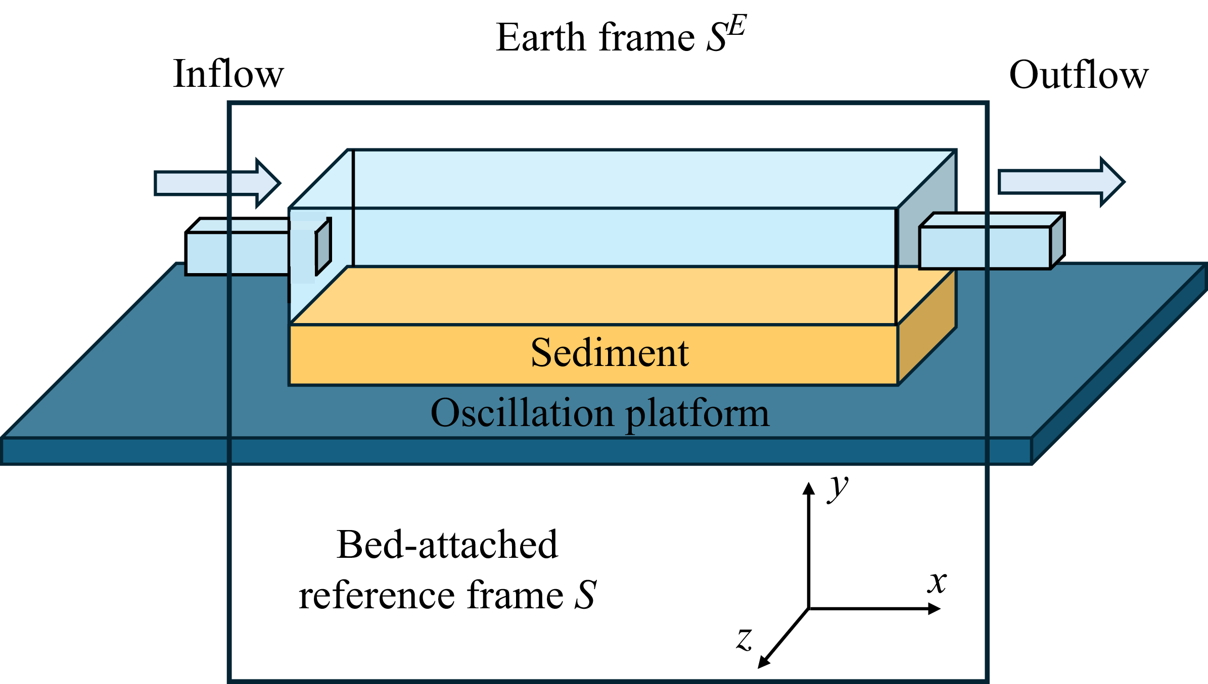
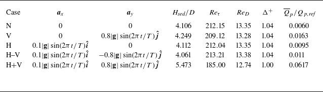
 Hsed
 §
 Qp
 Qp,ref
 §


 y=Hsed
 u′2¯
 v′2¯
 w′2¯
 ⋅
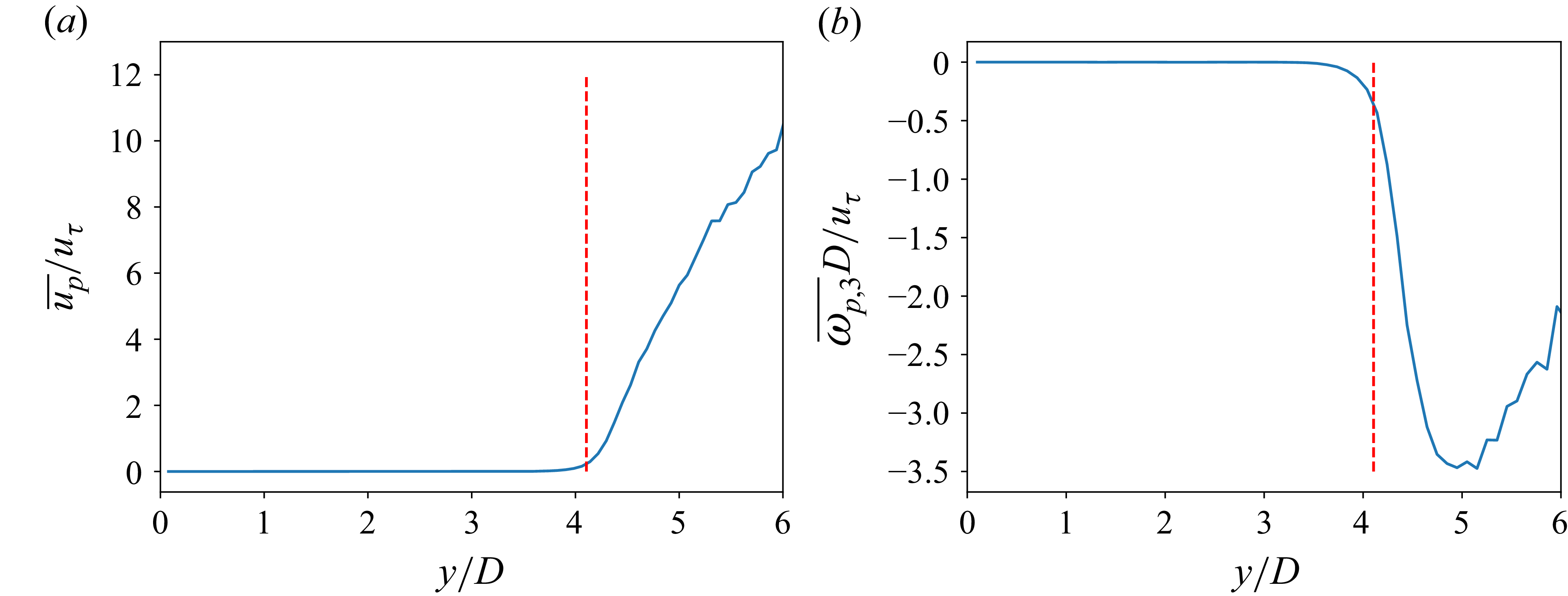
 0
 y=Hsed
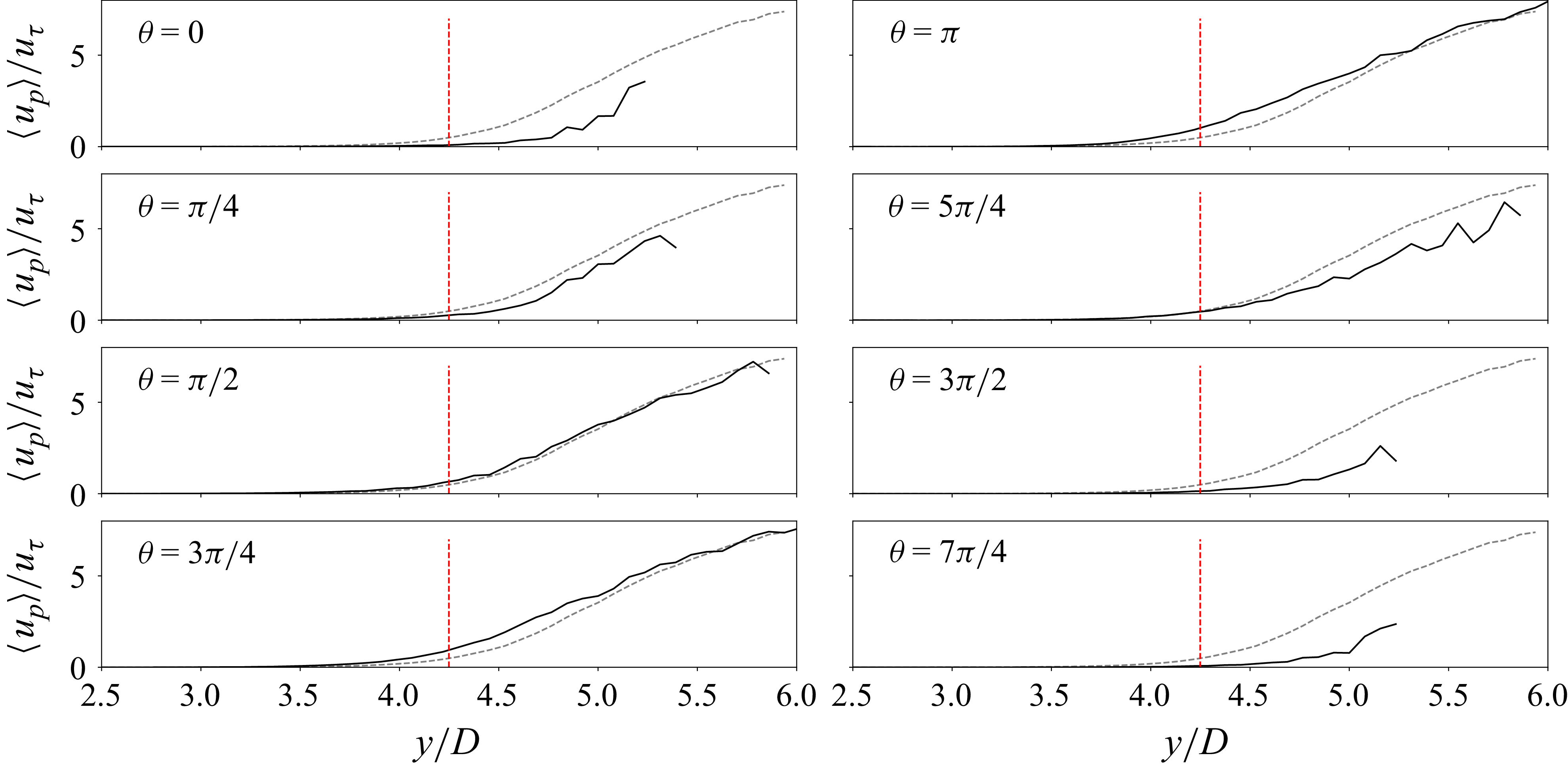
 u¯p(y)

 y=Hsed

 ⟨u′2⟩
 ⟨v′2⟩
 ⟨w′2⟩
 ⋅
 y=Hsed

 u¯(y)
 u¯p(y)
 u¯r(y)

 ⟨u′2⟩
 ⟨v′2⟩
 ⟨w′2⟩
 ⋅
 y=Hsed

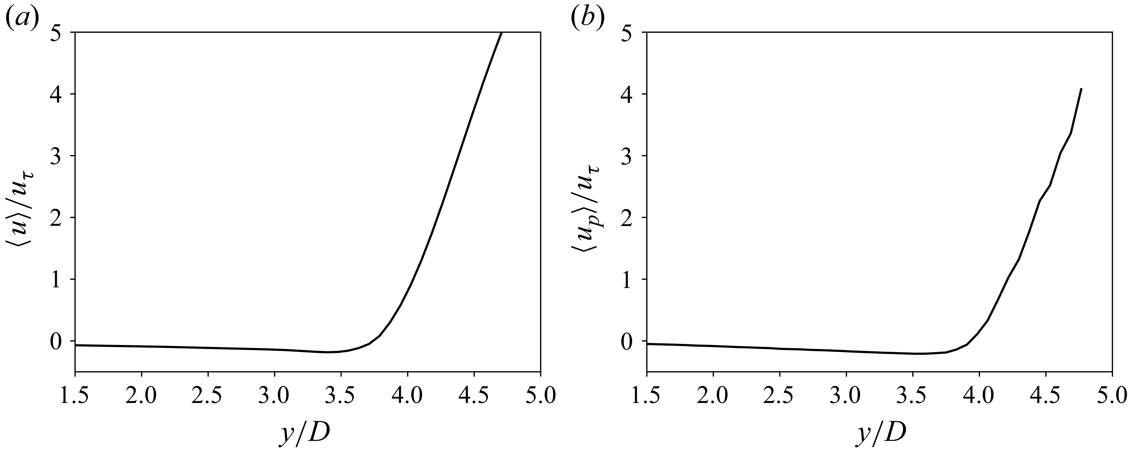
 θ=3π/2

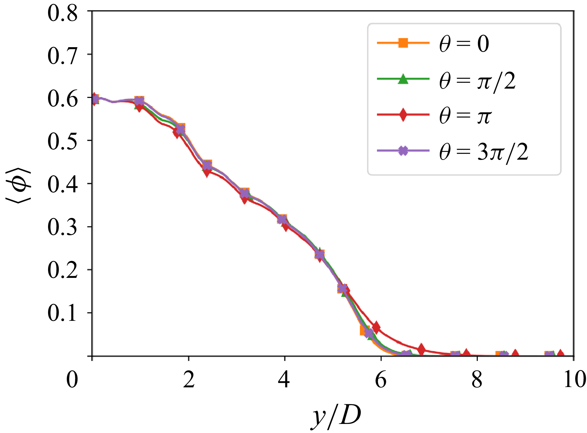
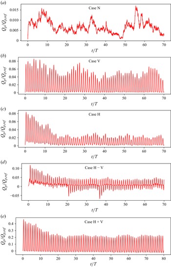
 T
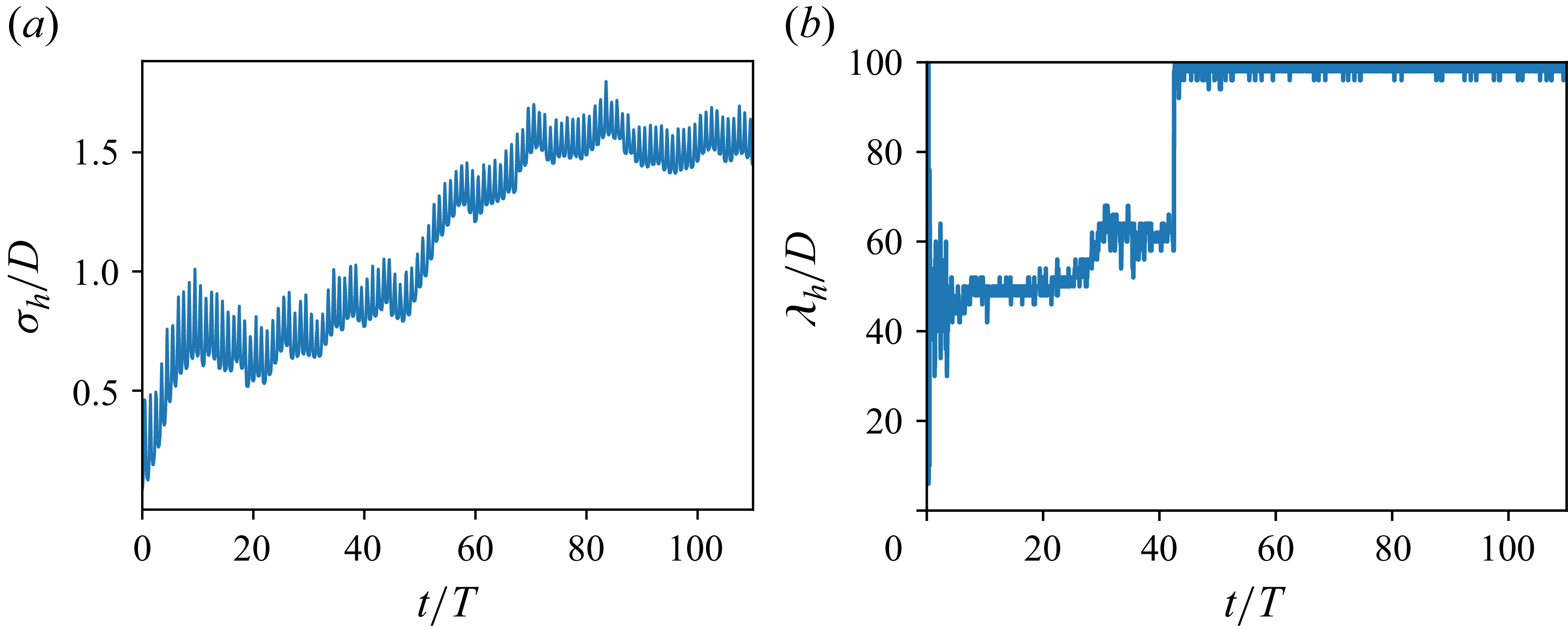
 σh
 λh


 τν(Hsed,θ)
 τR(Hsed,θ)
 ΩD(θ)

 ShM
 Sha
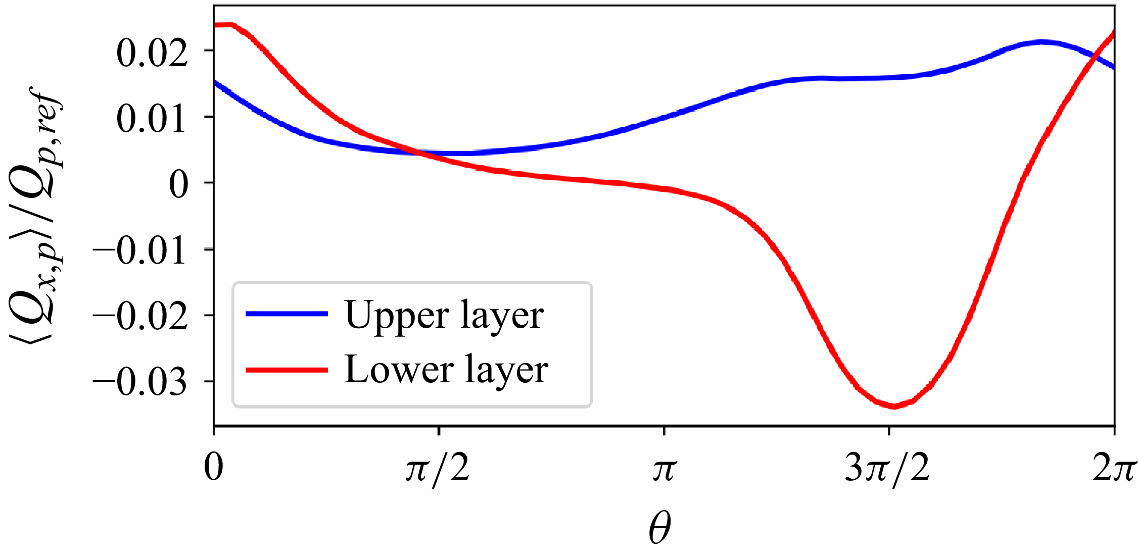

 ϕ¯
 u¯/uτ
 ui′2¯/uτ
 u′2¯
 v′2¯
 w′2¯
 ⋅


 Open access

