1. Introduction
Systemic risk refers to risks that have the potential to disrupt the entire market, economic system, or financial system, which distinguishes it from risks specific to individual firms or industries. Such risks often stem from macroeconomic factors, political events, and global challenges, resulting in widespread and profound consequences (Bisias et al., Reference Bisias, Flood, Lo and Valavanis2012; Feinstein et al., Reference Feinstein, Rudloff and Weber2017; Dičpinigaitienė and Novickytė, Reference Dičpinigaitienė and Novickytė2018). In today’s globalized economic environment, a deep understanding of systemic risk and effective management strategies are of paramount importance.
Systemic risk is commonly assessed through risk measures, among which value-at-risk (VaR) and expected shortfall (ES) are widely recognized (Duffie and Pan, Reference Duffie and Pan1997; Acerbi and Tasche, Reference Acerbi and Tasche2002). These risks are typically closely tied to global economic, financial, and political dynamics, resulting in widespread repercussions (Zhang and Cheung, Reference Zhang and Cheung2020; Duarte and Eisenbach, Reference Duarte and Eisenbach2021; Zhang et al., Reference Zhang, Wei, Lee and Tian2023). With advancements in research, alternative risk measurement frameworks have been developed, and the interdependence of risks has become a central theme in quantitative risk analysis (Goovaerts et al., Reference Goovaerts, Kaas and Laeven2011; Asimit and Gerrard, Reference Asimit and Gerrard2016; Yang et al., Reference Yang, Chen and Yuen2024). Since the 2008 financial crisis, risk measures have been increasingly employed to evaluate marginal risks (Kritzman et al., Reference Kritzman, Li, Page and Rigobon2010; Asimit and Li, Reference Asimit and Li2018; Liu and Yang, Reference Liu and Yang2021). Some studies have introduced conditional risk (co-risk) measures and risk contribution frameworks to assess systemic risk and quantify the interconnections among multiple economies.
Traditional risk measures, such as VaR and ES, have inherent limitations as they primarily focus on individual risk entities and overlook the interdependencies among economic agents. To address this limitation, various approaches have been proposed in the literature to measure systemic risk, aiming to quantify potential losses arising from financial contagion.
One of the most widely used systemic risk measures is conditional value-at-risk (
 $\mathrm{CoVaR}^=$
), initially introduced by Tobias and Brunnermeier (Reference Tobias and Brunnermeier2016):
 \begin{equation*} \text{CoVaR}_{\alpha,\beta}^{=}[Y|X] = \text{VaR}_\beta[Y | X = \text{VaR}_\alpha[X]],\end{equation*}
which assesses the
 $\beta$
-quantile of Y given that X equals its
 $\alpha$
-quantile.Footnote
1
To improve its empirical feasibility, Girardi and Ergün (Reference Girardi and Ergün2013) proposed the tail-based formulation CoVaR:
 \begin{equation*} \text{CoVaR}_{\alpha,\beta}[Y|X] = \text{VaR}_\beta[Y | X \gt \text{VaR}_\alpha[X]],\end{equation*}
which conditions on a nonzero probability event and is more robust in practice. Building on CoVaR, Mainik and Schaanning (Reference Mainik and Schaanning2014) introduced conditional expected shortfall (CoES), defined as
 \begin{equation*} \text{CoES}_{\alpha,\beta}[Y|X] = \frac{1}{1-\beta} \int_\beta^1 \text{CoVaR}_{\alpha,t}[Y|X] \, \mathrm{d} t.\end{equation*}
This measure captures the average of the most extreme losses in the conditional distribution of Y given X, providing a more stable and comprehensive evaluation of systemic risk than CoVaR alone.
Beyond CoVaR and CoES, several other systemic risk measures have been proposed. Acharya et al. (Reference Acharya, Pedersen, Philippon and Richardson2017) introduced systemic expected shortfall (SES) and marginal expected shortfall (MES), demonstrating that SES increases with institutional leverage. More recently, Dhaene et al. (Reference Dhaene, Laeven and Zhang2022) developed conditional distortion risk measures (CoD), where different distortion functions yield various systemic risk measures, encompassing well-established ones such as VaR and ES. Theoretical properties, as well as financial and insurance applications of these co-risk measures, have been extensively studied in previous works (see, e.g., Billio et al., Reference Billio, Getmansky, Lo and Pelizzon2012; Brownlees et al., Reference Brownlees and Engle2012; Benoit et al., Reference Benoit, Colletaz, Hurlin and Pérignon2013; Drakos and Kouretas, Reference Drakos and Kouretas2015; Mezei and Sarlin, Reference Mezei and Sarlin2016; Gong et al., Reference Gong, Liu, Xiong and Zhang2019; Zhang et al., Reference Zhang, Zhao and Cheung2019; Brogi et al., Reference Brogi, Lagasio and Riccetti2021; Rivera-Escobar et al., Reference Rivera-Escobar, Escobar and Manotas2022), offering valuable insights into systemic risk assessment and mitigation strategies.
These co-risk measures primarily assess the impact of one entity on another but do not fully capture absolute or relative spillover effects. This limitation has spurred research into developing various risk contribution measures to quantify the transmission of systemic risk more effectively. Girardi and Ergün (Reference Girardi and Ergün2013) define an institution’s systemic risk contribution as the change in its CoVaR across different states, denoted as
 $\Delta$
CoVaR. Sordo et al. (Reference Sordo, Bello and Suárez-Llorens2018) establish sufficient conditions for comparing conditional risk measures, such as CoVaR and CoES, as well as risk contribution measures like
 $\Delta$
CoVaR and
 $\Delta$
CoES. A distortion-based risk contribution measure (
 $\Delta$
CoD) is introduced by Dhaene et al. (Reference Dhaene, Laeven and Zhang2022), who analyze its theoretical properties and provide sufficient conditions for ranking
 $\Delta$
CoD. More recently, Zhang (Reference Zhang2024) propose several ratio-based distortion risk contribution measures (
 $\rm \Delta^R CoD$
) and investigate conditions for their comparative analysis.
Classical definitions typically rely on two types of conditioning events: one is the point condition
 $X = \text{VaR}_\alpha[X]$
, corresponding to
 $\text{CoVaR}^=$
; the other is the tail condition
 $X \gt \text{VaR}_\alpha[X]$
, corresponding to CoVaR. While the former offers clear theoretical interpretation, it is difficult to estimate under a continuous setting. The latter is more feasible in practice but may include extreme observations that obscure the characteristics of typical risk regions. In particular, during periods of economic expansion, occasional extreme events (such as “black swans”) may lead to inflated assessments of systemic risk. To more robustly capture “high-risk but non-extreme” systemic states, this paper introduces conditional risk measures based on quantile intervals–CoIVaR and CoIES (see Definition 3.1). The central idea is to define the conditioning event as
 ${\text{VaR}_{\alpha_1}[X] \lt X \leq \text{VaR}_{\alpha_2}[X]}$
, thereby assessing the potential loss of the individual variable Y when the systemic variable X falls within a “moderate-to-high risk” range. This framework can be viewed as a unified generalization: as
 $\alpha_1 \to \alpha_2^-$
, the interval event approximates the point condition and recovers
 $\text{CoVaR}^=$
; when
 $\alpha_2 \to 1^-$
, the interval condition degenerates to the upper-tail event, coinciding with CoVaR. In contrast, CoIVaR improves the estimability and interpretability of the risk measure, avoiding false alarms driven by extreme outliers.
The use of interval conditioning events offers greater operational feasibility in both risk management and capital allocation practices. For example, in financial markets, the event “the market drops exactly 5%” is nearly unobservable, while “the market drops more than 5%” may include extreme declines, potentially leading to upward-biased assessments of systemic risk. In contrast, CoIVaR, which is based on the condition that “market losses fall between 5% and 8%,” can more effectively capture typical periods of systemic stress–excluding the interference of extreme outliers while retaining key tail risk information. This enhances both the stability and interpretability of the risk measure.
In the context of capital allocation, the point-based condition based on VaR suffers from low estimation accuracy and slow convergence. To address this, Asimit et al. (Reference Asimit, Peng, Wang and Yu2019) proposed an ES-based allocation method, which transforms the classical VaR allocation problem into an estimation problem under the ES framework by adjusting the probability level. Building on this, the interval-based conditioning proposed in this paper can serve as a theoretical foundation for capital allocation. By retaining information about high-risk states while avoiding dominance by extreme values, this framework enhances the stability and practical applicability of the allocation rules. This connection also broadens the application prospects of interval-based risk measures in real-world regulation and financial risk management. For related discussions, see also Koike et al. (Reference Koike, Saporito and Targino2022) and Vernic (Reference Vernic2018).
As an expectation-based extension of CoIVaR, CoIES not only inherits its robustness but also captures the extreme loss risk under the conditional distribution, thereby offering more comprehensive support for risk assessment and regulatory decision-making. Based on this proposed framework, we conduct a systematic theoretical analysis and establish sufficient conditions for comparing risk vectors from the perspectives of marginal distributions, dependence structures, and stochastic orderings. To demonstrate the practical value of our theoretical results, we provide numerical simulation studies and apply our proposed methods to empirical stock market data. The findings indicate that the proposed measures are effective in identifying systemic risk and hold promising applications in financial risk management.
The remainder of this paper is organized as follows. Section 2 reviews key concepts and definitions. Section 3 introduces the definitions and properties of conditional interval risk measures. Section 4 explores the comparison of two random vectors under conditional interval risk measures, providing sufficient conditions for pairwise comparisons. In Section 5, we demonstrate the practical relevance of the proposed measures by applying them to stock market data in the context of systemic risk assessment. Finally, Section 6 concludes the paper with a summary of the main findings and suggests directions for future research.
2. Preliminaries
In this paper, let X and Y be two random variables with distribution functions F and G, respectively, denoted as “
 $X \sim F$
” and “
 $Y \sim G$
”. Their corresponding survival functions are
 $\overline{F}$
and
 $\overline{G}$
, while their density functions are f and g. We assume that all random variables under consideration are continuous, and all expectations and integrals exist whenever required. In addition, all bivariate random vectors are assumed to be absolutely continuous, and the associated copula functions admit the partial derivatives involved in the main results.
2.1. Stochastic orders
The stochastic order is a fundamental theoretical concept in probability theory, primarily used to compare the relative magnitudes of different random variables through probabilistic measures.
Definition 2.1. Let X and Y be two random variables with distribution functions F and G, respectively. Then X is said to be smaller than Y in the:
-
(i) usual stochastic order (denoted by
 $ X \leq_{\mathrm{st}} Y$
) if
${\overline F}(t) \leq {\overline G}(t)$
for all
$t \in {\mathbb R}$
;
-
(ii) likelihood ratio order (denoted by
$ X\leq_{\mathrm{lr}} Y$
) if
$g(t)/f(t)$
is increasing in
$t \in{\mathbb R}$
; -
(iii) dispersive order (denoted by
$ X\leq_{\mathrm{disp}} Y$
) if
$F^{-1}(p) - F^{-1}(q) \leq G^{-1}(p) - G^{-1}(q)$
for all
$0 \lt q \leq p \lt 1$
; -
(iv) excess wealth order (denoted by
$X\leq_{\mathrm{ew}} Y$
) if
$\mathbb{E}\left( X - F^{-1}(p) \right)_+ \le \mathbb{E}\left( Y - G^{-1}(p) \right)_+$
for all
$0 \lt p \lt 1$
, where
$x_+=\max(0,x)$
; -
(v) increasing convex (concave) order (denoted by
$X\leq_{\mathrm{icx[icv]}} Y$
) if
${\mathbb E}\left[ {\phi (X)} \right)]\leq {\mathbb E}\left[ {\phi (Y)} \right]$
for any increasing convex (concave) function
$\phi\,:\, \mathbb R\rightarrow \mathbb R$
; -
(vi) star order (denoted by
$ X\leq_{*} Y$
) if
$G^{-1}(p)/F^{-1}(p)$
is increasing in
$p \in (0,1)$
, when the two random variables are nonnegative; -
(vii) expected proportional shortfall order (denoted by
$X\leq_{\mathrm{ps}} Y$
) if
$\mathrm{EPS}_p(X) \leq \mathrm{EPS}_p(Y)$
for all
$p \in D_X\cap D_Y$
, when the two random variables are nonnegative, where
$D_X = \{p\in (0,1)\,:\,F^{-1}(p)\gt 0\}$
,
$D_Y = \{p\in (0,1)\,:\,G^{-1}(p)\gt 0\}$
. Here,
\begin{equation*}\mathrm{EPS}_{p}(X)=\mathbb{E}\left[ \left( \frac{X-\mathrm{VaR}_{p}(X)}{\mathrm{VaR}_{p}(X)}\right) _{+}\right] \text{ and }\mathrm{EPS}_{p}(Y)=\mathbb{E}\left[ \left( \frac{Y-\mathrm{VaR}_{p}(Y)}{\mathrm{VaR}_{p}(Y)}\right) _{+}\right] ;\end{equation*}
-
(viii)
$\mathcal{A}$
-stochastic dominance order (denoted by
$X \leq_{\mathcal{A}-\rm st}Y$
) if
$\mathbb{E}[\phi(X) \mid \mathcal{A}] \leq \mathbb{E}[\phi(Y) \mid \mathcal{A}]$
holds for every increasing function
$\phi \,:\, \mathbb{R} \to \mathbb{R}$
, where
$ \mathcal{A} $
is a
$ \sigma $
-field.





















For bivariate random variables (X, Y), a similar concept also exists, meaning that larger values of one component are associated with larger values of the other in some stochastic sense.
Definition 2.2. Let X and Y be two random variables with distribution functions F and G, respectively. Then,
-
(i) the bivariate random vector (X, Y) is said to be totally positive (reverse regular) of order 2 (denoted by
$\mathrm{TP}_{2}[\mathrm{RR}_{2}]$
) if
$\left[ X|Y=y_{1}\right]\leq _{\mathrm{lr}} \left[ \geq _{\mathrm{lr}} \right] \left[ X|Y=y_{2}\right] $
for all
$y_{1}\leq y_{2}$
, and
$\left[ Y|X=x_{1}\right] \leq _{\mathrm{lr}} \left[ \geq _{\mathrm{lr}} \right] \left[ Y|X=x_{2}\right] $
for all
$x_{1}\leq x_{2}$
; -
(ii) X is said to be stochastically increasing (decreasing) in Y (denoted by
$X\uparrow _{\mathrm{SI[SD]}}Y$
) if
$\left[ X|Y=y_{1}\right] \leq _{\mathrm{SI[SD]}} \left[ \geq _{\mathrm{SI[SD]}} \right] \left[ X|Y=y_{2}\right] $
for all
$y_{1}\leq y_{2}$
; -
(iii) the bivariate random vector (X, Y) is said to be positively (negatively) dependent through stochastic ordering (denoted by
${\mathrm{PDS [NDS]}}$
) if
$X\uparrow _{\mathrm{SI[SD]}} Y$
and
$Y\uparrow _{\mathrm{SI[SD]}} X$
; -
(iv) X is said to be right tail increasing (decreasing) in Y (denoted by
$X\uparrow_{\mathrm{RTI[RTD]}}\ Y$
) if
${\mathbb{P}}\left(X\gt x|Y\gt y\right) $
is increasing (decreasing) in
$y\in \mathbb{R}$
, for all
$x\in \mathbb{R}$
.












According to Shaked and Shanthikumar (Reference Shaked and Shanthikumar2007), bivariate random variables have the following relationships:
 $(X, Y)\,\text{is} \,\mathrm{TP}_2 \Rightarrow X \uparrow_{\mathrm{SI}} Y\,\text{and}\,Y \uparrow_{\mathrm{SI}} X \Rightarrow X \uparrow_{\mathrm{RTI}} Y\,\text{and}\,Y \uparrow_{\mathrm{RTI}} X.$
2.2. Copula
Let (X, Y) be a random vector with a joint distribution function H, denoted as
 $(X, Y) \sim H(x, y)$
. The function H can be expressed in terms of its copula representation as
 \begin{equation}H(x,y)=C(F(x),G(y)),\,\, x,y \in \mathbb R,\end{equation}
where C is the copula function defined on
 ${(0,1)^2}$
, characterizing the dependence structure between X and Y. If F and G are continuous, then C is uniquely determined by
 \begin{equation*}C(u,v)=H\left(F^{-1}(u),G^{-1}(v)\right),\,\, (u,v) \in {(0,1)^2}.\end{equation*}
The joint tail function
 $\overline{C}$
of two uniform random variables with copula C(u,v) is given by
 \begin{equation*}\overline C(u,v) = \mathbb{P}(U\gt u,V\gt v)=1-u-v+C(u,v),\,\,(u,v) \in {(0,1)^2}.\end{equation*}
Based on the above, the concordance order is defined as follows.
Definition 2.3. Given two copulas C and
 $C^{'}$
, C is smaller than
 $C^{'}$
in concordance order (denoted by
 $C\prec C^{'}$
) if
 $C(u,v)\leq C^{'}(u,v)$
, for all
 $(u,v) \in {(0,1)^2}$
.
The concordance order, also known as the correlation order or positive quadrant dependence (PQD) order (Dhaene and Goovaerts, Reference Dhaene and Goovaerts1996), defines a partial ordering on copulas. It provides a systematic framework for comparing the dependence structures of two random variables, particularly in assessing whether their joint cumulative distribution functions exhibit similar increasing trends.
We begin by briefly introducing several commonly used copulas. The Farlie–Gumbel–Morgenstern (FGM) copula is defined as
 $$C_{\theta(u,v)} = uv(1+\theta(1-u)(1-v)), \quad \theta \in[{-}1,1].$$
The copula is symmetric and commonly used to model weak dependence between variables. Specifically, when
 $\theta \gt 0$
, the variables tend to take larger or smaller values simultaneously. In other words,
 $C_{\theta}$
is
 $\mathrm{TP}_2$
for
 $\theta \in [0,1]$
, and
 $C_{\theta}$
is
 $\mathrm{RR}_2$
for
 $\theta \in [{-}1,0)$
.
A flexible and widely used class of copulas is the Archimedean family, defined via a generator function
 $\varphi\,:\, [0,1] \to [0, \infty)$
that is continuous, strictly decreasing, convex, and satisfies
 $\varphi(1) = 0$
. The general form of a bivariate Archimedean copula is
 \begin{align*}C(u,v) = \varphi^{-1}(\varphi(u) + \varphi(v)), \quad (u,v) \in [0,1]^2,\end{align*}
where
 $\varphi^{-1}$
denotes the pseudo-inverse of the generator function. Prominent members of this family include the Clayton copula, which captures strong lower tail dependence; the Gumbel copula, which models upper tail dependence; and the Ali–Mikhail–Haq (AMH) copula, which is known for its bounded dependence and analytical tractability. Due to their flexibility and interpretability, Archimedean copulas are widely applied in finance, insurance, and reliability.
3. Co-interval risk measures and related contribution measures
In this section, we introduce risk measures that extend across a range of confidence levels
 $(\alpha_1, \alpha_2)$
, namely the conditional interval (co-interval) value-at-risk and conditional interval expected shortfall (CoIES). Their definitions and key properties are as follows.
Definition 3.1. For given confidence levels
 $0 \lt \alpha_1 \lt \alpha_2 \lt 1$
and
 $\beta \in(0,1)$
, the conditional interval value-at-risk (
 ${\mathrm{CoIVaR}}$
) is defined as:
 \begin{equation} \mathrm{CoIVaR}_{\alpha_{1}-\alpha_{2},\beta }[Y|X]=\mathrm{VaR}_{\beta} \left[ Y|\mathrm{VaR}_{\alpha_{1}}[X] \lt X\leq \mathrm{VaR}_{\alpha_{2}}[X]\right].\end{equation}
Similarly, the
 $\mathrm{CoIES}$
is given by
 \begin{equation} \mathrm{CoIES}_{\alpha_1-\alpha_2, \beta}[Y|X] = \frac{1}{1 - \beta} \int_{\beta}^{1} \mathrm{CoIVaR}_{\alpha_1 - \alpha_2,t}[Y|X]dt.\end{equation}
CoIVaR and CoIES are conditional interval (co-interval) risk measures that differ from traditional co-risk metrics by evaluating the risk of the variable Y conditioned on the event
 $\{\mathrm{VaR}_{\alpha_1}[X] \lt X \leq \mathrm{VaR}_{\alpha_2}[X]\}.$
This construction naturally arises when estimating conditional quantiles, such as
 $ \mathrm{VaR}_\beta[Y \mid X = \mathrm{VaR}_\alpha(X)] $
, particularly in the continuous case where the conditioning event has zero probability, making it difficult to observe and estimate directly. In contrast, CoIVaR is relatively easier to estimate and compute since it relies on observable intervals and conditional information. By allowing
 $ \alpha_1 \to \alpha_2^- $
, the interval condition serves as a practical approximation, providing a useful alternative to direct estimation. Furthermore, during periods of economic expansion, restricting the conditioning event to the interval
 $ (\alpha_1, \alpha_2) $
helps mitigate the overestimation of systemic risk caused by rare extreme events. This improves the robustness and interpretability of the risk measure, making it more applicable in real-world scenarios.
Furthermore, the co-interval risk contribution measure can be formally defined. For any given co-interval risk measure, the corresponding contribution measure is expressed as follows.
Definition 3.2. For given
 $0 \lt \alpha_1 \lt \alpha_2 \lt 1$
and
 $\beta \in(0,1)$
, two types of risk contribution measures are defined:
-
(i) The co-interval value-at-risk contribution measures (
$\Delta \mathrm{CoIVaR}$
) and
\begin{equation*}\Delta \mathrm{CoIVaR}_{\alpha_1 - \alpha_2,\beta}[Y|X] = \mathrm{CoIVaR}_{\alpha_1 - \alpha_2,\beta}[Y|X] - \mathrm{VaR}_\beta[Y]\end{equation*}
\begin{equation*}\Delta^{\mathrm{med}} \mathrm{CoIVaR}_{\alpha_1 - \alpha_2,\beta}[Y|X] = \mathrm{CoIVaR}_{\alpha_1 - \alpha_2,\beta }[Y|X] - \mathrm{CoIVaR}_{1/2 - \alpha_2,\beta}[Y|X].\end{equation*}
-
(ii) The co-interval expected shortfall contribution measures (
$\Delta \mathrm{CoIES}$
) and
\begin{equation*}\Delta \mathrm{CoIES}_{\alpha_1 - \alpha_2,\beta}[Y|X] = \mathrm{CoIES}_{\alpha_1 - \alpha_2,\beta}[Y|X] -\mathrm{ES}_\beta[Y]\end{equation*}
\begin{equation*}\Delta^{\mathrm{med}} \mathrm{CoIES}_{\alpha_1- \alpha_2,\beta}[Y|X] = \mathrm{CoIES}_{\alpha_1 - \alpha_2,\beta }[Y|X] - \mathrm{CoIES}_{1/2 -\alpha_2,\beta}[Y|X].\end{equation*}


Risk contribution measures quantify the spillover effects of risk by evaluating the difference between the risk of a given entity and a benchmark value, as discussed by Sordo et al. (Reference Sordo, Bello and Suárez-Llorens2018) and Dhaene et al. (Reference Dhaene, Laeven and Zhang2022). One common approach involves assessing this contribution by comparing the conditional interval risk measure with its corresponding unconditional risk level. Alternatively, the median state of X can serve as a benchmark condition for calculating the contribution, offering an alternative perspective on the transmission of systemic risk.
Next, a co-interval risk contribution ratio measure is introduced to quantify the relative spillover effects arising from systemic risk.
Definition 3.3. For given
 $0 \lt \alpha_1 \lt \alpha_2 \lt 1$
and
 $\beta \in(0,1)$
, the co-interval risk contribution ratio measures are defined as follows:
-
(i) The co-interval value-at-risk contribution ratio measures (
$\Delta^{\mathrm{R}} \mathrm{CoIVaR}$
) provided that
\begin{equation*}\Delta^{\mathrm{R}} \mathrm{CoIVaR}_{\alpha_1 - \alpha_2,\beta}[Y|X] =\frac{ \mathrm{CoIVaR}_{\alpha_1 - \alpha_2,\beta}[Y|X] - {\mathrm{VaR}}_\beta[Y]}{ {\mathrm{VaR}}_\beta[Y]}\end{equation*}
$ \mathrm{VaR}_\beta[Y] \ne 0$
, and provided that
\begin{equation*}\Delta^{\mathrm{R-med}} \mathrm{CoIVaR}_{\alpha_1 - \alpha_2,\beta}[Y|X] =\frac{ \mathrm{CoIVaR}_{\alpha_1 - \alpha_2,\beta}[Y|X] - {\mathrm{CoIVaR}}_{1/2 - \alpha_2,\beta}[Y|X]}{ {\mathrm{CoIVaR}}_{1/2 - \alpha_2,\beta}[Y|X]}\end{equation*}
$ \mathrm{CoIVaR}_{1/2 - \alpha_2,\beta}[Y|X] \ne 0$
.
-
(ii) The co-interval expected shortfall contribution ratio measures (
$\Delta^{\mathrm{R}} \mathrm{CoIES}$
) provided that
\begin{equation*}\Delta^{\mathrm{R}} \mathrm{CoIES}_{\alpha_1 - \alpha_2,\beta}[Y|X] = \frac{\mathrm{CoIES}_{\alpha_1 - \alpha_2,\beta}[Y|X] - \mathrm{ES}_\beta[Y]}{\mathrm{ES}_\beta[Y]}\end{equation*}
$ \mathrm{ES}_\beta[Y] \ne 0$
, and provided that
\begin{equation*}\Delta^{\mathrm{R-med}} \mathrm{CoIES}_{\alpha_1 - \alpha_2,\beta}[Y|X] = \frac{\mathrm{CoIES}_{\alpha_1 - \alpha_2,\beta}[Y|X] - \mathrm{CoIES}_{1/2 -\alpha_2,\beta}[Y|X]}{\mathrm{CoIES}_{1/2 -\alpha_2,\beta}[Y|X]}\end{equation*}
$ \mathrm{CoIVaR}_{1/2 - \alpha_2,\beta}[Y|X] \ne 0$
.






The risk contribution ratio measures evaluate the marginal impact of individual institutions on overall systemic risk. By capturing the relative difference between an entity’s conditional risk exposure at a given risk level and its inherent risk, these measures facilitate an assessment of risk relative spillovers across the financial network. For further insights on risk contribution measures, readers are referred to Pu et al. (Reference Pu, Zhang and Zhang2024) and Zhang (Reference Zhang2024).
To assess the theoretical soundness of the proposed measures, we examine whether CoIVaR and CoIES satisfy the four axioms of coherent risk measures–translation invariance, monotonicity, positive homogeneity, and subadditivity (Artzner et al., Reference Artzner, Delbaen, Eber and Heath1999). Specifically, CoIES satisfies all four axioms and thus qualifies as a coherent risk measure, while CoIVaR satisfies the first three but fails subadditivity in general. However, it retains comonotonic additivity under certain conditions. Detailed formulations and proofs of these properties are provided in online supplementary material. Moreover, the constructions of CoIVaR, CoIES, and interval-based conditioning events can also be applied to capital allocation problems. Preliminary discussions and potential research directions in this regard are provided in online supplementary material.
4. Comparison results for two bivariate risk vectors
If
 $h \, : \, [0,1] \rightarrow[0,1]$
is an increasing function such that
 $h(0) = 0$
and
 $h(1) = 1$
, then h is referred to as a distortion function. The collection of all such distortion functions is denoted by
 $\mathcal{G}$
.
Definition 4.1. The distortion risk measure
 $D_g$
for a random variable X with distribution function F, and distortion function
 $g \in \mathcal{G}$
, is defined as
 \begin{equation*}D_g[X] = \int_0^{+ \infty} g\left(\overline{F}(t) \right)\mathrm{d}t + \int_{- \infty}^0 \left[g\left(\overline{F}(t)\right) - 1 \right] \mathrm{d}t = \int_0^1 F^{-1}(t) \mathrm{d}\overline{g}(t),\end{equation*}
where
 $\overline{g}(t) = 1 - g(1 - t)$
, referred to as the dual distortion function of g(t). Clearly,
 $\overline{g}(t)\,:\, [0,1] \mapsto [0,1]$
is also a distortion function. If X is a nonnegative random variable, then
 $D_g$
simplifies to
 \begin{equation*}D_g[X] = \int_0^{+ \infty} g\left(\overline{F}(t)\right)\mathrm{d}t.\end{equation*}
For a left-continuous distortion function g, the transformation of the tail function
 $\overline{F}$
of X, given by
 $g(\overline{F}(x)) = g \circ \overline{F}(x)$
, defines a new tail function associated with a random variable
 $X_g$
. Using the distortion function, we now derive the following lemma.
Lemma 4.2. Let (X, Y) be a bivariate random vector with copula C, and marginal distributions F and G, respectively. For given
 $u_0 \lt \alpha_1 \lt \alpha_2 \lt 1$
, if
 $\partial_2^2 C(\alpha_1, v) \leq \partial_2^2 C(\alpha_2, v)$
for all
 $v \in (0,1)$
, where
 $ \partial_2^2 C(u,v)\,:\!=\,\frac{\partial^2C(u,v)}{\partial v^2}$
. Then the conditional random variable
 $[Y|\mathrm{VaR}_{\alpha_1}[X] \lt X \leq \mathrm{VaR}_{\alpha_2}[X]]$
is a distortion random variable derived from Y and the concave distortion function
 \begin{equation} h_{\alpha_1-\alpha_2}(t) = \frac{\overline C(\alpha_1,1 - t) - \overline C(\alpha_2,1-t)}{\alpha_2 - \alpha_1}.\end{equation}
Note that the condition
 $\partial_2^2 C(\alpha_1,v) \leq \partial_2^2 C(\alpha_2,v)$
implies that the conditional probability
 $\mathbb P(\alpha_1 \lt U \leq \alpha_2 \mid V = v)$
is increasing in v. This indicates that as the individual variable V approaches its upper tail, the likelihood of the systemic variable U falling within the interval
 $(\alpha_1, \alpha_2]$
increases, revealing a pattern in which systemic tail risk intensifies in response to extreme individual shocks. In particular, when
 $\alpha_2 = 1$
, the interval corresponds to the upper tail region of the systemic variable. This condition characterizes a mechanism of tail risk co-amplification, which reflects the contagion effect of systemic risk.
The following lemma presents an alternative expression for CoIVaR, which will be utilized in the subsequent comparison of results.
Lemma 4.3. Let (X, Y) be a random vector with copula C, and marginal distribution functions F and G, respectively. Assuming that F is continuous, then
 \begin{equation*}\mathrm{CoIVaR}_{\alpha_1-\alpha_2,\beta}[Y|X] = G^{-1}\left(1-h^{-1}_{\alpha_1-\alpha_2} (1-\beta)\right),\end{equation*}
where
 $h_{\alpha_1-\alpha_2}(t)$
is defined in (4.1).
For two random vectors (X, Y) and (X
′, Y
′), the spillover effects of risks under different conditions can be compared. The following theorem provides sufficient conditions for comparing
 $ \mathrm{CoIVaR}_{\alpha_1 - \alpha_2, \beta }[Y|X] $
and
 $ \mathrm{CoIVaR}_{\alpha_1 - \alpha_2, \beta }[Y'|X'] $
under the usual stochastic order.
Theorem 4.4. Let (X, Y) and (X′, Y′) be two random vectors with distribution functions F, G and F′, G′, and copulas C and C′, respectively. Assume that there exists
 $u_0 \in (0,1)$
such that
 $\partial_1 C(u,v) \geq \partial_1 C'(u,v)$
for all
 $u \gt u_0$
and
 $v\in(0,1)$
Footnote
2
, where
 $\partial_1 C(u,v)\,:\!=\,\frac{\partial C(u,v) }{\partial u}$
. Then, for given
 $u_0 \lt \alpha_1 \lt \alpha_2 \lt 1$
,
 $Y \leq_{\mathrm{st}} Y'$
implies that
 \begin{equation} \mathrm{CoIVaR}_{\alpha_1 - \alpha_2, \beta }[Y|X] \leq \mathrm{CoIVaR}_{\alpha_1 - \alpha_2, \beta}[Y'|X'].\end{equation}
Here,
 $\partial_1C(u, v) = \mathbb P(V \leq v \mid U = u)$
represents the probability that the individual variable V falls below the threshold v given the system state
 $U = u$
. Therefore,
 $\partial_1C(u, v) \geq \partial_1C'(u, v)$
implies that, under the same system condition, the individual faces lower right-tail risk under copula C than under C
′. In other words, copula C
′ exhibits stronger right-tail dependence and systemic contagion effect.
Next, we present several examples of copulas that satisfy the two main conditions considered in this paper:
 $\partial_1 C(u,v) \geq \partial_1 C'(u,v)$
for all
 $u \gt u_0$
and
 $v \in (0,1)$
;
 $\partial_2^2 C(\alpha_1, v) \leq \partial_2^2 C(\alpha_2, v)$
for all
 $v \in (0,1)$
.
Example 4.5. Consider the FGM copula. Its first and second partial derivatives are given by
 \begin{equation*}\partial_1 C(u,v) = v \left( 1 + \theta (1 - 2u)(1 - v) \right), \quad\partial_2^2 C(u,v) = -2\theta u(1 - u).\end{equation*}
Let
 $u_0 = \frac{1}{2} $
. For
 $u_0 \lt \alpha_1 \lt \alpha_2 \lt 1 $
and
 $\theta\geq 0 $
, the inequality
 $\partial _{2}^{2}C(\alpha _{1},v)\leq \partial _{2}^{2}C(\alpha _{2},v)$
holds for all
 $v \in (0,1) $
. According to Lemma 4.2, this implies that the distortion function
 $h_{\alpha_1 - \alpha_2}(t) $
, defined in equation (4.1), is concave. Moreover, consider another FGM copula
 $C^{\prime }(u,v)=uv\left( 1+\theta^{\prime }(1-u)(1-v)\right) $
, with dependence parameter
 $\theta ^{\prime }$
. Then, the inequality
 $\partial _{1}C(u,v)\geq \partial _{1}C^{\prime }(u,v)$
holds if either
 $u\gt u_{0}$
and
 $0\lt \theta \leq \theta ^{\prime }$
, or
 $u\lt u_{0}$
and
 $\theta \geq \theta ^{\prime }\gt 0$
. These results confirm that the FGM copula satisfies the sufficient conditions required in Theorem 4.4.
For Archimedean copulas, due to the complexity of their analytical forms, it is difficult to verify the conditions explicitly. Therefore, following the approach in Zhang (Reference Zhang2024), we investigate whether two Archimedean copulas–Clayton and AMH–satisfy the conditions under tail-dependent parameter settings through numerical evaluations and graphical illustrations.
Example 4.6. The Clayton copula, defined by
 \begin{align*}C(u,v) = \left( u^{-\theta} + v^{-\theta} - 1 \right)^{-1/\theta}, \quad \theta \in (0, +\infty),\end{align*}
is generated by the function
 $\varphi(t) = t^{-\theta} - 1$
. Let C and C′ denote Clayton copulas with parameters
 $\theta = 0.4$
and
 $\theta' = 0.6$
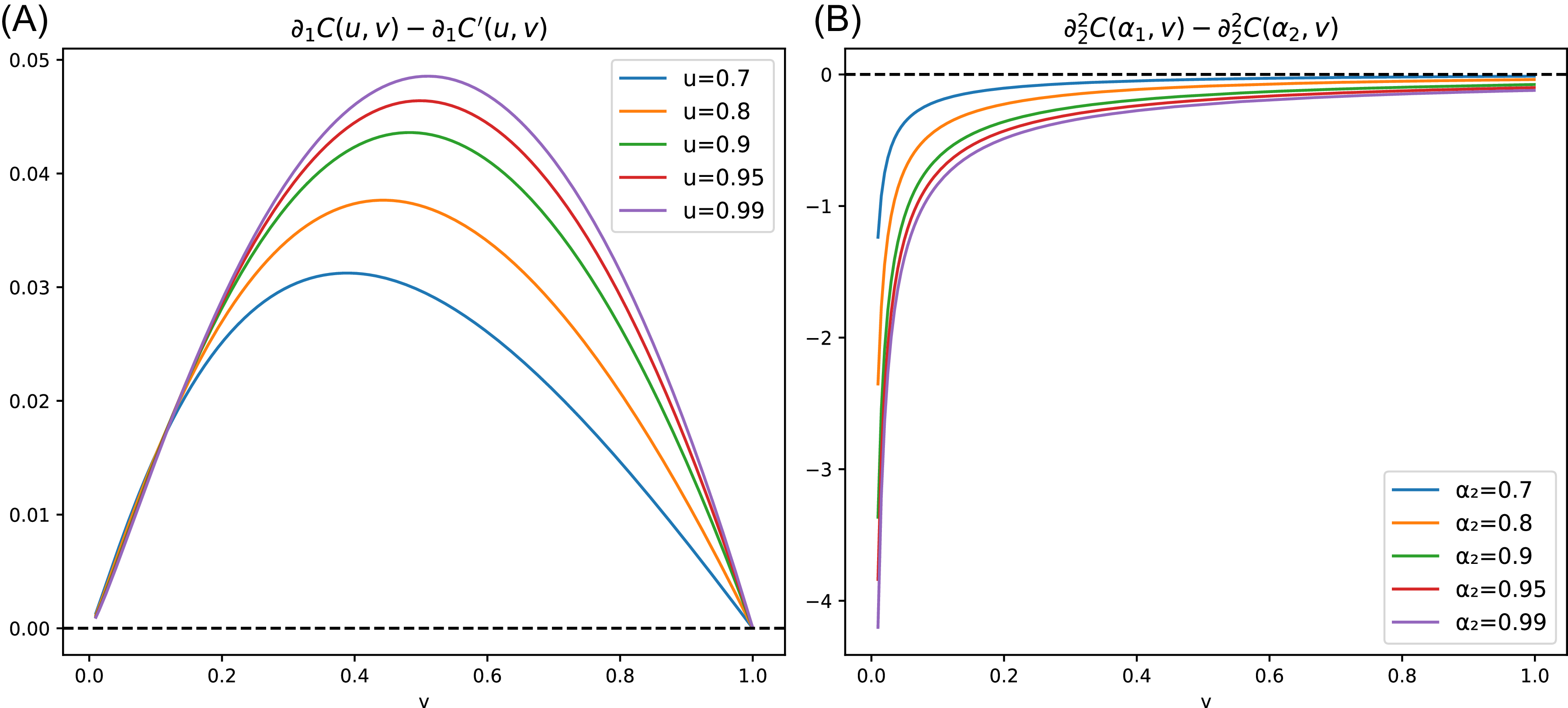
, respectively. Figure 1(a) plots the difference
 $\partial_1 C(u,v) - \partial_1 C'(u,v)$
as a function of
 $v \in (0,1)$
for various values of u. The results show that the inequality
 $\partial_1 C(u,v) \geq \partial_1 C'(u,v)$
holds under this parameter setting, thereby verifying the condition required in Theorem 4.4. Figure 1(b) presents the second-order derivative
 $\partial_2^2 C(\alpha, v)$
for
 $\alpha_1 = 0.6$
and various
 $\alpha_2 \gt \alpha_1$
. The observed inequality
 $\partial_2^2 C(\alpha_1, v) \leq \partial_2^2 C(\alpha_2, v)$
, holding for all
 $v \in (0,1)$
, confirms that the sufficient condition in Lemma 4.2 is also satisfied.
Clayton copula.

Example 4.7. Another notable member of the Archimedean family is the AMH copula, defined by the generator function
 $\varphi(t) = \ln \left( \frac{1 - \theta(1 - t)}{t} \right)$
. Its explicit form is given by
 \begin{align*}C(u,v)=\frac{uv}{1-\theta(1-u)(1-v)}, \quad \theta \in [{-}1,1).\end{align*}
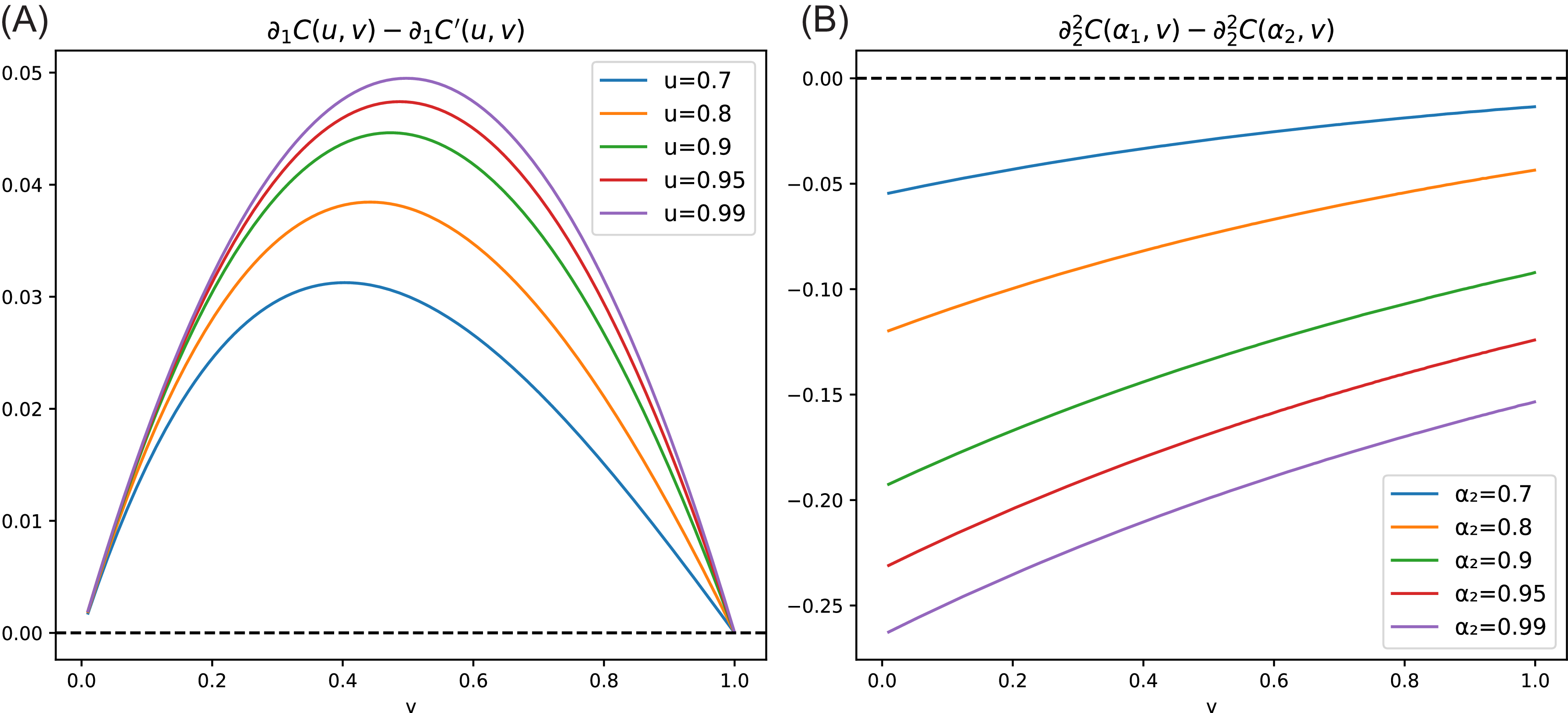
Under the same parameter setting as in Example 4.6, the AMH copula exhibits similar behavior. As shown in Figure 2, these results further confirm that the sufficient conditions required in Lemma 4.2 and Theorem 4.4 hold under the tail-dependent parameter configuration.
Ali–Mikhail–Haq copula.

The following results on the usual stochastic order and the increasing convex order, as discussed by Sordo and Ramos (Reference Sordo and Ramos2007), are summarized below. These will be used to establish partial results in this paper.
Lemma 4.8. Assuming X and Y are two random variables with distribution functions F and G, respectively. Then,
 $X \leq_{\mathrm{icx}} Y$
if and only if
 \begin{equation*}\int^1_0 F^{-1}(t) dA(t) \leq \int^1_0 G^{-1}(t) dA(t),\end{equation*}
for all increasing convex functions
 $A\,:\, [0,1]\rightarrow R$
.
The following theorem provides sufficient conditions for comparing
 $ \mathrm{CoIES}_{\alpha_1 - \alpha_2, \beta }[Y|X] $
and
 $ \mathrm{CoIES}_{\alpha_1 - \alpha_2, \beta }[Y'|X'] $
in the usual stochastic order and increasing convex order.
Theorem 4.9. Let (X, Y) and (X′, Y′) be two random vectors with copulas C and C′, and marginal distributions F, G and F′, G′, respectively. Assume there exists
 $u_0 \in (0,1)$
such that
 \begin{align*}\partial_1 C(u,v) \geq \partial_1 C'(u,v), \quad \forall u \gt u_0, \; v \in (0,1).\end{align*}
For any
 $u_0 \lt \alpha_1 \lt \alpha_2 \lt 1$
, if either
-
(i)
$Y \leq_{\mathrm{st}} Y'$
, or -
(ii)
$Y \leq_{\mathrm{icx}} Y'$
and
$\partial_2^2 C(\alpha_1, v) \leq \partial_2^2 C(\alpha_2, v)$
for all
$v \in (0,1)$
, then
\begin{align*}\mathrm{CoIES}_{\alpha_1 - \alpha_2, \beta}[Y|X] \leq \mathrm{CoIES}_{\alpha_1 - \alpha_2, \beta}[Y'|X'].\end{align*}





It is known that
 $Y \leq_{\mathrm{st}} Y'$
implies
 $Y \leq_{\mathrm{icx}} Y'$
. Thus, according to Theorem 4.9, when replacing the condition
 $Y \leq_{\mathrm{st}} Y'$
with the weaker condition
 $Y \leq_{\mathrm{icx}} Y'$
, the conclusion still holds under the newly imposed conditions. To compare risk contribution measures, the following lemma is introduced.
Example 4.10. Let (X, Y) and (X′, Y′) be two random vectors associated with FGM copulas C and C′, corresponding to parameters
 $\theta$
and
 $\theta'$
, respectively. Let
 $Z \sim N(\mu, \sigma^2)$
denote a normal distribution with location parameter
 $\mu \in \mathbb{R}$
and scale parameter
 $\sigma \gt 0$
. Suppose
 $Y \sim N(\mu_1, \sigma_1^2)$
and
 $Y' \sim N(\mu_2, \sigma_2^2)$
, with
 $\mu_1\leq \mu_2$
and
 $\sigma_1 = \sigma_2$
, which implies
 $Y \leq_{\mathrm{ st}} Y'$
(see Table 2.1 of Belzunce et al., Reference Belzunce, Riquelme and Mulero2015). For
 $0 \lt \theta \lt \theta'$
and
 $u \gt 1/2$
, we have
 $\partial_1 C(u, v) \gt \partial_1 C'(u, v)$
. Since this satisfies the condition in Theorem 4.4, it follows that
 $\mathrm{CoIVaR}_{\alpha_1 - \alpha_2, \beta}[Y | X] \leq \mathrm{CoIVaR}_{\alpha_1 - \alpha_2, \beta}[Y'| X'].$
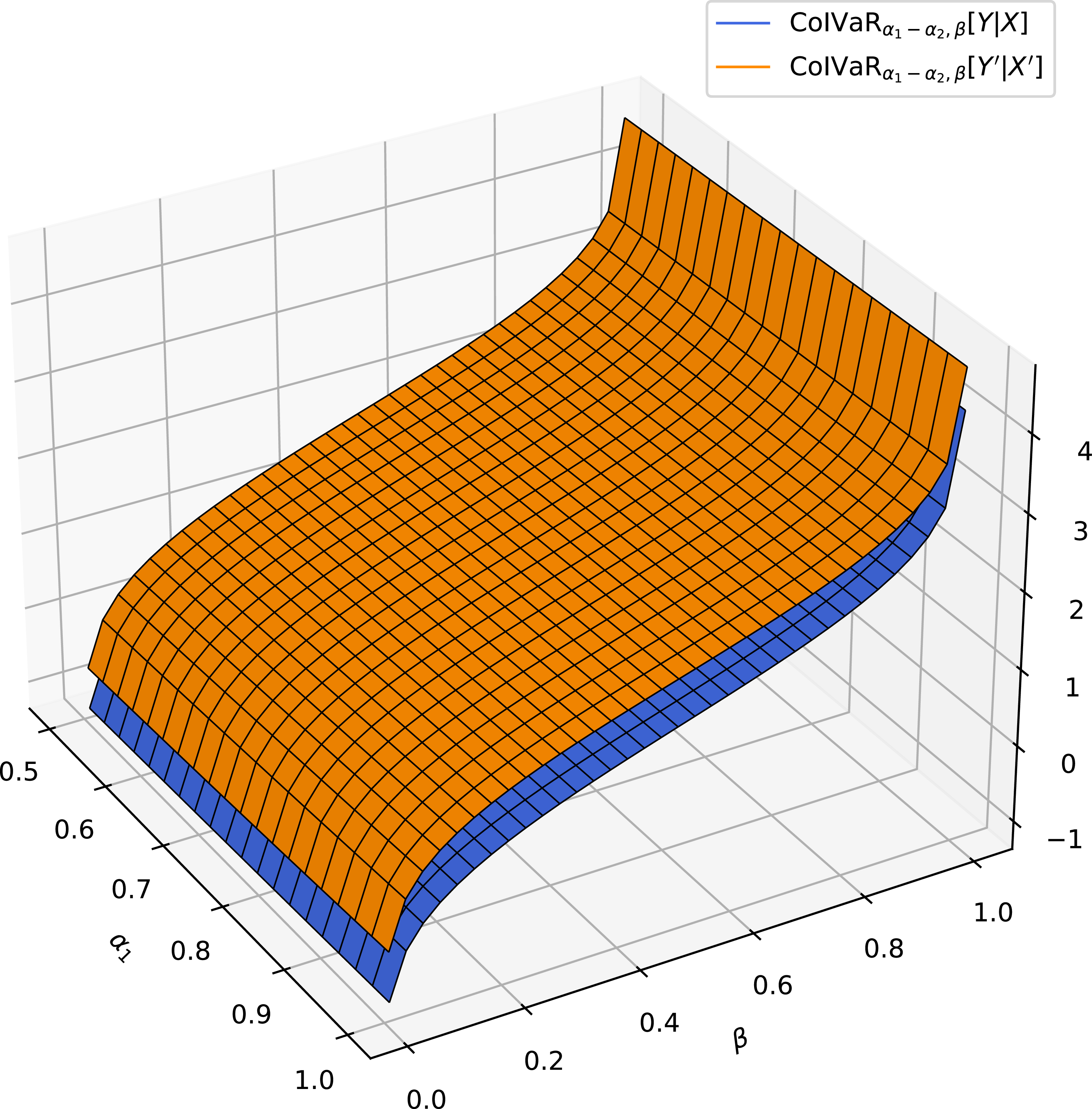
Figure 3 illustrates this result for a specific parameter setting.
Comparison of
 $\mathrm{CoIVaR}_{\alpha_1 - \alpha_2, \beta}[Y | X] $
and
 $\mathrm{CoIVaR}_{\alpha_1 - \alpha_2, \beta}[Y'| X']$
as functions of
 $\alpha_1$
and
 $\beta$
, with
 $\alpha_2=0.99$
,
 $Y \sim N(1,1)$
,
 $Y'\sim N(1.5,1)$
,
 $\theta = 0.4$
, and
 $\theta' = 0.6$
.

Example 4.11. Let (X, Y) and (X′, Y′) be two random vectors associated with FGM copulas C and C′, corresponding to parameters
 $\theta$
and
 $\theta'$
, respectively. Let
 $Z \sim G(a, b)$
denote a Gamma distribution with shape parameter
 $a \gt 0$
and scale parameter
 $b \gt 0$
. Suppose
 $Y \sim G(a_1, b_1)$
and
 $Y' \sim G(a_2, b_2)$
with
 $a_1 \gt a_2$
and
 $a_1 b_1 \leq a_2 b_2$
, which implies
 $Y \leq_{\mathrm{icx}} Y'$
(see Table 2.2 of Belzunce et al., Reference Belzunce, Riquelme and Mulero2015). Combining this with Example 4.10, where
 $Y \leq_{\mathrm{st}} Y'$
and
 $\partial_1 C(u,v) \gt \partial_1 C'(u,v)$
holds for
 $0 \lt \theta \lt \theta'$
and
 $u \gt 1/2$
, the conditions of Theorem 4.9 are satisfied. Consequently, we obtain
 $\mathrm{CoIES}_{\alpha_1 - \alpha_2, \beta }[Y|X] \leq \mathrm{CoIES}_{\alpha_1 - \alpha_2, \beta }[Y'|X'].$
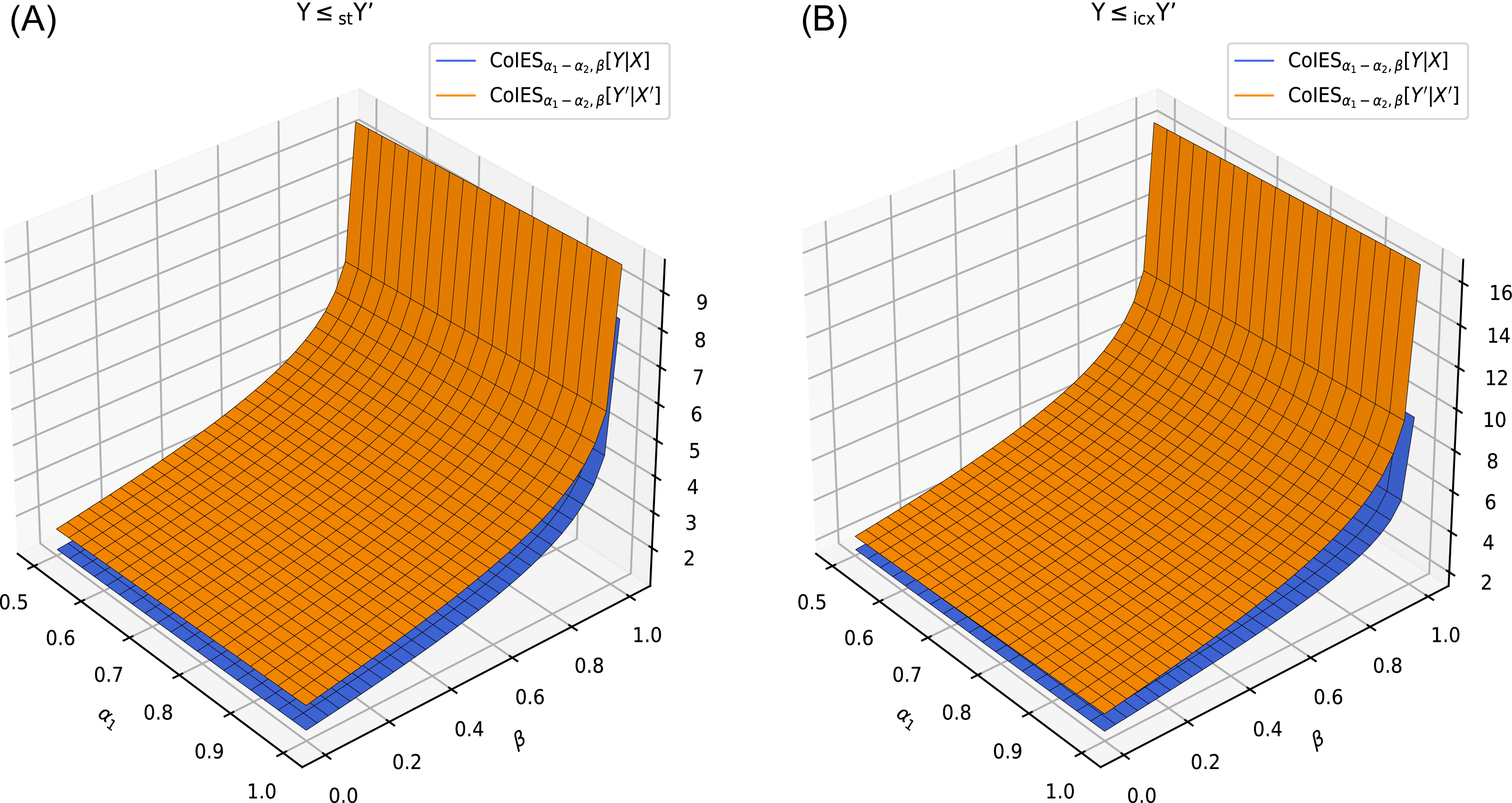
Figure 4 illustrates this result for specific parameter settings.
Comparison of
 $\mathrm{CoIES}_{\alpha_1 - \alpha_2, \beta }[Y|X]$
and
 $\mathrm{CoIES}_{\alpha_1 - \alpha_2, \beta }[Y'|X']$
as functions of
 $\alpha_1$
and
 $\beta$
, with
 $\alpha_2 = 0.99$
,
 $\theta = 0.4$
, and
 $\theta' = 0.6$
. Subfigure A:
 $Y \sim N(1,1)$
,
 $Y' \sim N(1.5,1)$
; Subfigure B:
 $Y \sim G(1.5, 1)$
,
 $Y' \sim G(1, 2)$
.

Lemma 4.12. (Sordo et al., Reference Sordo, Bello and Suárez-Llorens2018). Let X and Y be two continuous random variables with distribution functions F and G, respectively. Suppose h and g are distortion functions, where h is concave and satisfies
 $h(t) \leq g(t)$
for all
 $t \in [0, 1]$
. Denote
 $X_h$
as the distorted random variable induced by X and
 $h({\cdot})$
, and
 $Y_g$
as the distorted random variable induced by Y and
 $g({\cdot})$
. Then,
 $X \leq_{\mathrm{disp}} Y$
implies
-
(i)
$F^{-1}_{X_h}(p)-F^{-1}(p) \leq F^{-1}_{Y_g}(p)- G^{-1}(p)$
, for all
$p \in (0,1)$
; -
(ii)
$F^{-1}_{X_g}(p)-F^{-1}_{X_h}(p) \leq F^{-1}_{Y_g}(p)- F^{-1}_{Y_h}(p)$
, for all
$p \in (0,1)$
.




The following theorem provides sufficient conditions for comparing the risk contribution measures of
 $\Delta \mathrm{CoIVaR}_{{\alpha_1} - {\alpha_2},\beta}[Y|X]$
and
 $\Delta \mathrm{CoIVaR}_{{\alpha_1} - {\alpha_2},\beta}[Y'|X']$
in the dispersive order.
Theorem 4.13. Let (X, Y) and (X′,Y′) be two random vectors with copulas C and C′, respectively. The marginal distributions are F, G and F′, G′, respectively. Assume there exists
 $u_0 \in (0,1)$
such that for all
 $v \in (0,1)$
, we have
 $\partial_1 C(u,v) \geq \partial_1 C'(u,v)$
for all
 $u \gt u_0$
, and
 $\partial_2^2 C(\alpha_1,v) \leq \partial_2^2 C(\alpha_2,v)$
for all
 $u_0 \lt \alpha_1 \lt \alpha_2 \lt 1$
. Then
 $Y \leq_{\mathrm{disp}} Y' $
implies
 \begin{equation} \Delta \mathrm{CoIVaR}_{{\alpha _1} - {\alpha _2},\beta }[Y|X] \leq \Delta \mathrm{CoIVaR}_{{\alpha _1} - {\alpha _2},\beta }[Y'|X'].\end{equation}
Assuming X is a random variable with distribution function F, Sordo (Reference Sordo2008) defined a class of risk measures as follows:
 \begin{equation*}\rho_{A,B}(X) = \int^1_0 F^{-1}(t) \mathrm{d}A(t) - \int^1_0 F^{-1}(t) \mathrm{d}B(t),\end{equation*}
where A(t) and B(t) are two distortion functions. These risk measures are used to characterize comparisons under the excess wealth order.
Lemma 4.14. (Sordo, Reference Sordo2008). Let X and Y be two random variables with distribution functions F and G, respectively. Then,
 $X \leq_{\mathrm{ew}} Y$
if and only if
 $\rho_{A,B}(X) \leq \rho_{A,B}(Y)$
for all
 $\rho_{A,B}$
such that B(t) and
 $A\circ B^{-1}(t)$
are convex.
Building on the lemma above, sufficient conditions are provided for comparing the risk contribution measures
 $\Delta \mathrm{CoIES}_{{\alpha_1} - {\alpha_2},\beta}[Y|X]$
and
 $\Delta \mathrm{CoIES}_{{\alpha_1} - {\alpha_2},\beta}[Y'|X']$
under the excess wealth order.
Theorem 4.15. Let (X, Y) and (X′,Y′) be two random vectors with copulas C and C′, respectively. The marginal distributions are F, G and F′, G′, respectively. Assume there exists
 $u_0 \in (0,1)$
such that for all
 $v \in (0,1)$
, we have
 $\partial_1 C(u,v) \geq \partial_1 C'(u,v)$
for all
 $u \gt u_0$
, and
 $\partial_2^2 C(\alpha_1,v) \leq \partial_2^2 C(\alpha_2,v)$
for all
 $u_0 \lt \alpha_1 \lt \alpha_2 \lt 1$
. Then,
 $Y \leq_{\mathrm{ew}} Y'$
implies
 \begin{equation} \Delta \mathrm{CoIES}_{{\alpha _1} - {\alpha _2},\beta }[Y|X] \leq \Delta \mathrm{CoIES}_{{\alpha _1} - {\alpha _2},\beta }[Y'|X'].\end{equation}
Example 4.16. Consider two bivariate random vectors (X, Y) and (X′, Y′), associated with FGM copulas C and C′, respectively, corresponding to parameters
 $\theta$
and
 $\theta'$
. Let
 $Z \sim W(a, b)$
denote a Weibull distribution with shape parameter
 $a\gt 0$
and scale parameter
 $b\gt 0$
. Suppose
 $Y \sim W(a_1, b_1)$
and
 $Y' \sim W(a_2, b_2)$
with
 $a_1 = a_2$
and
 $b_1 \leq b_2$
, which implies
 $Y \leq_{\mathrm{disp}} Y'$
; Suppose
 $Y \sim G(a_1, b_1)$
and
 $Y' \sim G(a_2, b_2)$
with
 $a_1 \leq a_2$
and
 $b_1 \leq b_2$
, which implies
 $Y \leq_{\mathrm{ew}} Y'$
(see Tables 2.1 and 2.2 of Belzunce et al., Reference Belzunce, Riquelme and Mulero2015). For
 $0 \lt \theta \lt \theta'$
and
 $u_0 = 1/2$
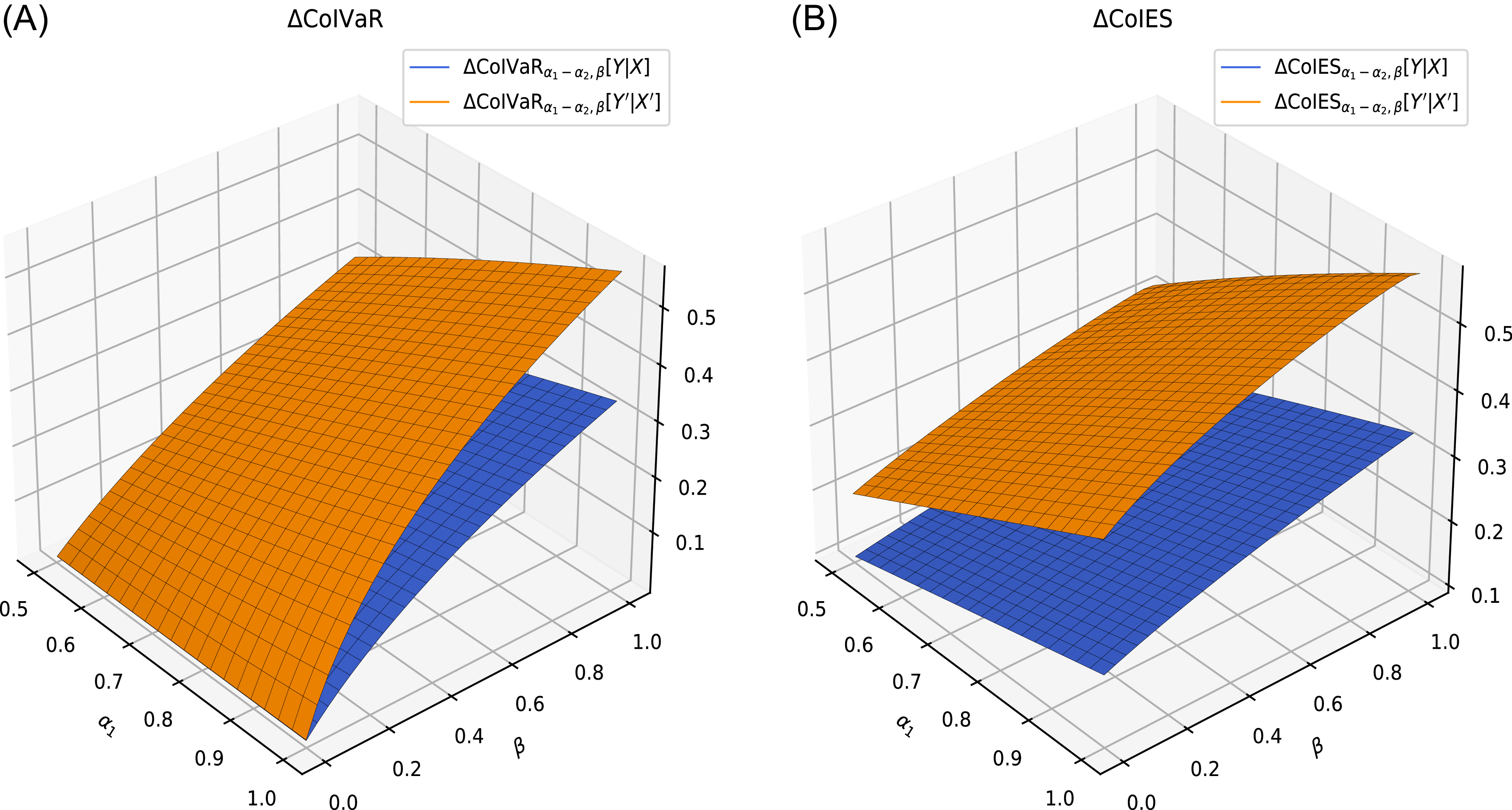
, the conditions of Theorems 4.13 and 4.15 are satisfied. Figure 5 illustrates this result for specific parameter settings.
Comparison of
 $\Delta \mathrm{CoIVaR}$
and
 $\rm \Delta CoIES$
as functions of
 $\alpha_1$
and
 $\beta$
, with
 $\alpha_2 = 0.99$
,
 $\theta = 0.4$
, and
 $\theta' = 0.6$
. Subfigure A:
 $Y \sim W(1, 1)$
,
 $Y' \sim W(1, 1.2)$
; Subfigure B:
 $Y \sim G(1, 1)$
,
 $Y' \sim G(1.2, 1.2)$
.

For fixed x
′, define the function
 $g(x, y) \,:\!=\, \mathbb{P}(x \lt X \leq x' \mid Y = y)$
. The function g(x, y) is said to be totally positive of order two (TP
 $_2$
) in (x, y) if, for all
 $x_1 \leq x_2\lt x'$
and
 $y_1 \leq y_2$
, the following inequality holds:
 $g(x_1, y_1)\, g(x_2, y_2) \geq g(x_1, y_2)\, g(x_2, y_1).$
This definition follows the characterization of TP
 $_2$
functions as discussed in Zhang (Reference Zhang2024). Next, we aim to establish sufficient conditions for comparing the risk contribution measures in the form of
 $\Delta^{\mathrm{med}} {\mathrm{CoIVaR}}_{\alpha_1 - \alpha_2, \beta}[Y|X]$
and
 $\Delta^{\mathrm{med}} {\mathrm{CoIES}}_{\alpha_1 - \alpha_2, \beta}[Y|X]$
.
Theorem 4.17. Let (X, Y) and (X′, Y′) be two random vectors with the same copula C. The marginal distributions are F, G and F′, G′, respectively. Assuming
 $1/2 \lt \alpha_1 \lt \alpha_2 \lt 1$
holds.
-
(i) Suppose
$Y \uparrow_{\mathrm{RTI}} X $
, then
$Y \leq_{\mathrm{disp}} Y'$
implies (4.5)
\begin{equation} \Delta^{\mathrm{med}} \mathrm{CoIVaR}_{{\alpha _1} - {\alpha _2},\beta } [Y|X] \leq \Delta^{\mathrm{med}} \mathrm{CoIVaR}_{{\alpha _1} - {\alpha _2},\beta }[Y'|X'],\end{equation}
-
(ii) Suppose
$g(x,y) = \mathbb P(x\lt X \leq x'|Y=y)$
is
$\mathrm{TP}_2$
, then
$Y \leq_{\mathrm{ew}} Y'$
implies (4.6)
\begin{equation} \Delta^{\mathrm{med}} \mathrm{CoIES}_{{\alpha _1} - {\alpha _2},\beta }[Y|X] \leq \Delta^{\mathrm{med}} \mathrm{CoIES}_{{\alpha _1} - {\alpha _2},\beta }[Y'|X'].\end{equation}





Next, sufficient conditions for comparing risk contribution ratio measures for two risk portfolios, (X, Y) and (X ′, Y ′), are provided. To simplify the proofs of the main results, the following lemma is introduced.
Lemma 4.18. (Belzunce et al., Reference Belzunce, Pinar, Ruiz and Sordo2012). Let X and Y be two random variables with distribution functions F and G, respectively. Then, the following hold:
-
(i)
$X \leq_{*} Y$
if and only if
$I_{A,B}(X) \leq I_{A,B}(Y)$
for all distortion functions A(t), B(t) and convex functions
$A \circ B^{-1}(t)$
; -
(ii)
$X \leq_{\mathrm{ps}} Y$
if and only if
$I_{A,B}(X) \leq I_{A,B}(Y)$
for all distortion functions A(t), convex distortion functions B(t) and
$A \circ B^{-1}(t)$
, where (4.7)
\begin{equation} I_{A,B}(X) = \frac{\int_0^1 F^{-1}(t) dA(t)}{\int_0^1 F^{-1}(t) dB(t)} -1 \,\,\text{and}\,\, I_{A,B}(Y) = \frac{\int_0^1 G^{-1}(t) dA(t)}{\int_0^1 G^{-1}(t) dB(t)} -1.\end{equation}







Building on the previous lemma, sufficient conditions for comparing the risk contribution ratio measures in the forms of
 $\Delta^{\mathrm{R}} \mathrm{ CoIVaR}_{\alpha_1 - \alpha_2, \beta}[Y|X]$
and
 $\Delta^{\mathrm{R}} {\mathrm{CoIES}}_{\alpha_1 - \alpha_2, \beta}[Y|X]$
are provided in the following theorem.
Theorem 4.19. Let (X, Y) and (X′, Y′) be two sets of risk random vectors with copulas C and C′, respectively. Their marginal distributions are F, G and F′, G′, respectively. Assume there exists
 $u_0 \in (0,1)$
such that for all
 $v \in (0,1)$
, the inequality
 $\partial_1 C(u,v) \geq \partial_1 C'(u,v)$
holds for all
 $u \gt u_0$
, and
 $\partial_2^2 C(\alpha_1,v) \leq \partial_2^2 C(\alpha_2,v)$
holds for all
 $u_0 \lt \alpha_1 \lt \alpha_2 \lt 1$
. Then,
-
(i)
$Y\leq _{\ast }Y^{\prime }$
implies (4.8)
\begin{equation}\Delta ^{\mathrm{R}}\mathrm{CoIVaR}_{{\alpha _{1}}-{\alpha _{2}},\beta}[Y|X]\leq \Delta ^{\mathrm{R}}\mathrm{CoIVaR}_{{\alpha _{1}}-{\alpha _{2}},\beta }[Y^{\prime }|X^{\prime }], \end{equation}
-
(ii)
$Y\leq _{\mathrm{ps}}Y^{\prime }$
implies (4.9)
\begin{equation}\Delta ^{\mathrm{R}}\mathrm{CoIES}_{{\alpha _{1}}-{\alpha _{2}},\beta}[Y|X]\leq \Delta ^{\mathrm{R}}\mathrm{CoIES}_{{\alpha _{1}}-{\alpha _{2}},\beta }[Y^{\prime }|X^{\prime }]. \end{equation}


Example 4.20. Let (X, Y) and (X′, Y′) be two random vectors with the FGM copulas C and C′, respectively. Suppose
 $Y \sim G(a_{1},b_{1})$
and
 $Y' \sim G(a_{2}, b_{2})$
with
 $a_{1} \geq a_{2}$
, which implies
 $Y {\leq_{{\star}}} Y'$
and
 $Y {\leq_{\mathrm{ps}}} Y'$
. For
 $0 \lt \theta \lt \theta'$
and
 $u_{0} = 1/2$
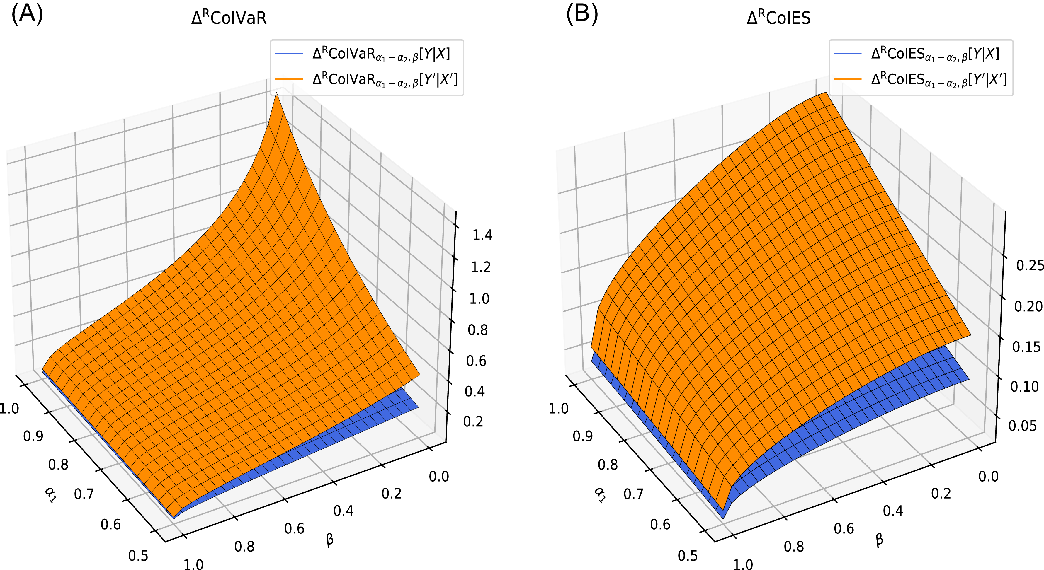
, the conditions of Theorem 4.19 are satisfied. Figure 6 illustrates this result for specific parameter settings.
Comparison of
 $\Delta^{\mathrm{R}}\mathrm{CoIVaR}$
and
 $\Delta^{\mathrm{R}} \mathrm{CoIES}$
as functions of
 $\alpha_{1}$
and
 $\beta$
, with
 $\alpha_{2} = 0.99$
,
 $Y \sim G(1.2,1)$
,
 $Y' \sim G(1,1)$
,
 $\theta = 0.4$
, and
 $\theta' = 0.6$
.

Sufficient conditions for comparing the risk contribution ratio measures
 $\Delta^{\mathrm{R-med}} \mathrm{CoIES}_{\alpha_{1} - \alpha_{2}, \beta}[Y|X]$
and
 $\Delta^{\mathrm{R-med}} \mathrm{CoIES}_{\alpha_{1} - \alpha_{2}, \beta}[Y'|X']$
are provided in the following theorem.
Theorem 4.21. Let (X, Y) and (X′, Y′) be two risk-related random vectors with a common copula C, and marginal distributions F, G and F′, G′, respectively. Assume that for some
 $1/2 \lt \alpha_{1} \lt \alpha_{2} \lt 1$
, the inequality
 $\partial_{2}^2 C(\alpha_{1}, v) \leq \partial_{2}^2 C(\alpha_{2}, v)$
holds for all
 $v \in (0,1)$
.
-
(i) If
$Y \uparrow_{\mathrm{RTI}} X$
, then
$Y \leq_* Y' $
implies
\begin{equation*} \Delta^{\mathrm{R-med}} \mathrm{CoIVaR}_{{\alpha _1} - {\alpha _2},\beta }[Y|X] \leq \Delta^{\mathrm{R-med}} {\mathrm{CoIVaR}}_{{\alpha _1} - {\alpha _2},\beta }[Y'|X'],\end{equation*}
-
(ii) If
$g(x,y) = \mathbb P(x\lt X\leq x'|Y=y)$
is TP2, then
$Y \leq_{\mathrm{ps}} Y' $
implies
\begin{equation*} \Delta^{\mathrm{R-med}} \mathrm{CoIES}_{{\alpha _1} - {\alpha _2},\beta }[Y|X] \leq \Delta^{\mathrm{R-med}} {\mathrm{CoIES}}_{{\alpha _1} - {\alpha _2},\beta }[Y'|X'].\end{equation*}





The results in Theorems 4.19 and 4.21 establish conditions for comparing risk contribution measures, such as
 $\Delta^{\mathrm{R}} \mathrm{ CoIVaR}$
and
 $\Delta^{\mathrm{R}} {\mathrm{CoIES}}$
, under various stochastic orders and dependence structures. These conditions highlight the role of marginal distributions and copulas in determining risk aggregation and contributions. The findings are important for risk management, particularly in assessing systemic risk and optimizing portfolio allocations, as they emphasize how changes in dependence structures influence risk exposure, especially in extreme events.
5. A real-world application in the stock market
5.1. Data and parameter estimation
This study selects the CSI 300 Index as the source of risk and five individual stocks–Kweichow Moutai (KWM), China Merchants Bank (CMB), China Yangtze Power (CYP), Jiangsu Hengrui Medicine (HRM), and Gree Electric Appliances (GEA) – as the affected entities. According to the WIND industry classification, these stocks belong to the consumer staples, financials, utilities, healthcare, and consumer discretionary sectors, respectively. According to WIND data as of December 31, 2024, these stocks rank among the top 20 A-share stocks by free-float market capitalization out of more than 5400 listed firms. As leading firms in their respective industries, they provide a suitable basis for analyzing cross-sectoral spillover effects under market shocks. The dataset covers the daily closing prices of the selected funds or stocks from January 1, 2007, to December 31, 2024, encompassing major market shocks such as the 2008 Global Financial Crisis and the COVID-19 pandemic in 2020. Based on the selected sample data, the log-loss is calculated as follows:
 \begin{equation} L_{i,t} = -100 \cdot\ln \left( \frac{p_{i,t}}{p_{i,t-1}} \right)\end{equation}
where
 $ p_{i,t} $
denotes the closing price of asset i on day t, and
 $ L_{i,t} $
represents its log-loss.
We use the generalized Pareto distribution (GPD) to fit the marginal distribution of the log-returns, with its cumulative distribution function given by:
 $G_{\xi,\eta}(x) = 1 - \left(1 + \xi \cdot \frac{x}{\eta}\right)^{-1/\xi},$
where
 $ \xi \neq 0 $
is the shape parameter and
 $ \eta \gt 0 $
is the scale parameter. Specifically, the GPD is applied to fit the tails of the log-returns, while the middle region is estimated using the empirical distribution, as described by Koliai (Reference Koliai2016):
 \begin{equation} F(x) = \left\{ \begin{array}{ll} \frac{N_{u_L}}{N} \left( 1 - \xi_L \cdot \frac{x - u_L}{\eta_L} \right)^{-1/\xi_L}, & x \le u_L, \\[6pt] \hat{F}(x), & u_L \lt x \leq u_R, \\[6pt] 1 - \frac{N_{u_R}}{N} \left( 1 + \xi_R \cdot \frac{x - u_R}{\eta_R} \right)^{-1/\xi_R}, & x \gt u_R, \end{array} \right.\end{equation}
where
 $ u_L $
and
 $ u_R $
represent the lower and upper threshold values,
 $ N_{u_L} $
and
 $ N_{u_R} $
are the number of observations exceeding these thresholds, and
 $ \hat{F}(x) $
denotes the empirical distribution function.
For copula function selection, considering that financial market data often exhibit tail dependence, we refer to the study by Christoffersen and Langlois (Reference Christoffersen and Langlois2013), which demonstrates that the Student’s t copula effectively captures asymmetry and dependence in financial data. Therefore, Student’s t copula is used to describe the dependence structure between different assets, expressed as follows:
 \begin{equation} C_{\rho, k}(u, v) = \frac{1}{2 \pi \sqrt{1 - \rho^2}} \int_{-\infty}^{t_k^{-1}(u)} \int_{-\infty}^{t_k^{-1}(v)} \left[ 1 + \frac{s^2 - 2 \rho s z + z^2}{k(1 - \rho^2)} \right]^{-\frac{k+2}{2}} \mathrm{d} s \mathrm{d} z,\end{equation}
where
 $ t_k^{-1}({\cdot}) $
denotes the inverse function of the Student’s t distribution with k degrees of freedom, and
 $\rho \in ({-}1, 1)$
is the correlation coefficient.
5.2. Static numerical results
The log-loss of the CSI 300 index and individual stocks was calculated based on (5.1), and their distributions were fitted using the GPD as specified in Equation (5.2). The lower and upper threshold values were selected as the 0.1 and 0.9 quantiles, respectively, following the methodology of Koliai (Reference Koliai2016). Figure S1 of the supplementary material presents the QQ plot based on (5.2), and the results indicate that the GPD provides a good fit for the tail distributions of both the index and individual stock log-losses.
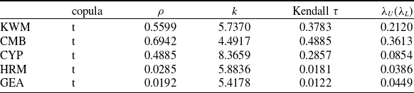
Next, based on the copula model in (5.3), the parameters between the CSI 300 index and the five selected stocks were estimated. The results are summarized in Table 1. Specifically,
 $ \rho $
represents the correlation coefficient, k denotes the degrees of freedom, Kendall’s
 $ \tau $
is used to measure the overall dependence between variables, and
 $ \lambda_U $
and
 $ \lambda_L $
represent the upper-tail and lower-tail dependence coefficients, respectively. The results indicate that KWM and CMB exhibit a strong correlation with the CSI 300 Index, suggesting that their volatility trends align closely with the overall market fluctuations. Notably, CMB shows a stronger tail dependence, implying higher risk under extreme market conditions. This may be related to its market position in the consumer goods and financial sectors, as well as its sensitivity to economic cycles. In contrast, HRM and GEA show lower tail dependence, reflecting the stability of their respective industries and their lower sensitivity to market fluctuations.
Copula parameters for CSI 300 and selected stocks.

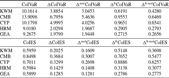
Risk measures for
 $\alpha_1 = 0.95$
,
 $\alpha_2= 1$
and
 $\beta = 0.95$
.
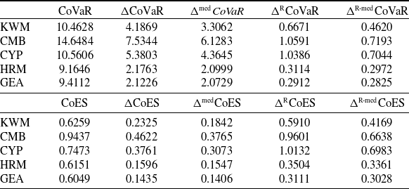
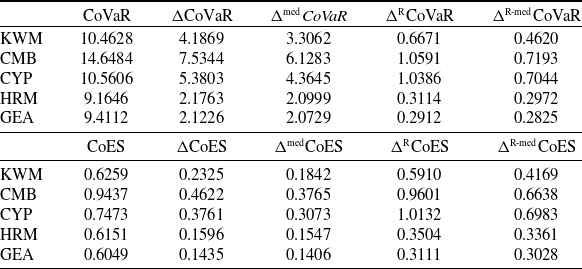
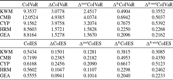
Based on the marginal distributions and copula functions of each asset, a series of risk measures were calculated, and the results are presented in Tables 2–4. In these tables,
 $\alpha_1 = 0.95$
and
 $\beta_2 = 0.95$
are fixed, while
 $\alpha_2$
is set to 1, 0.999, and 0.99, respectively, to analyze the risk exposures of the assets at different confidence levels. The following results are derived from the risk measures displayed in the tables.
-
(i) Under different parameter settings and risk measures, the five assets exhibit significant differences. In terms of absolute risk measures, CMB consistently shows higher risk values than the other assets, indicating greater tail risk. In contrast, HRM and GEA have lower risk values, suggesting that they are more resilient to extreme market fluctuations. Regarding relative risk measures, CYP exhibits higher risk, implying that for the same unit change in risk, CYP experiences greater tail risk. In practical asset management, appropriate strategies should be adopted based on the characteristics of each asset and specific management objectives.
-
(ii) The high-risk level exhibited by CMB is consistent with the results in Table 1. Its high lower tail dependence coefficient
$\lambda_L$
and correlation coefficient
$\rho$
indicate that this asset not only faces significant loss risk during extreme market downturns but also contributes substantially to systemic risk. Although CYP ranks third among all assets in terms of correlation and tail dependence coefficients, its lower tail dependence coefficient is significantly lower than that of KWM and CMB. This suggests that CYP has relatively weak tail dependence with the CSI 300 index under extreme market downturns. However, in terms of risk measures, CYP exhibits slightly higher risk metrics than KWM and demonstrates a more pronounced effect when measuring relative spillover effects. This finding suggests that relying solely on correlation and tail dependence coefficients to assess market co-movement may be insufficient. A more comprehensive evaluation requires considering the distributional characteristics of asset returns along with other risk indicators to better capture asset performance under different market conditions. -
(iii) The data trends indicate that as
$\alpha_2$
decreases, the risk measures exhibit a general downward trend, which is consistent with practical expectations. When
$\alpha_2$
approaches 1, more extreme risk events are incorporated into the decision-making process, leading investors to adopt a more cautious risk assessment, thereby increasing the estimated risk values. Conversely, a smaller
$\alpha_2$
reflects a reduced consideration of extreme events, resulting in relatively lower risk measure values. -
(iv) Across different confidence levels, the risk rankings of assets remain largely consistent for the same risk measure. This indicates a high degree of alignment between interval risk measures and traditional systemic risk measures such as CoVaR and CoES. Consequently, interval risk measures can serve as an effective alternative to conventional single confidence level risk measures. Compared to traditional approaches, this method offers greater flexibility in application and encompasses existing risk measures as special cases, making it particularly advantageous for capturing extreme market events.


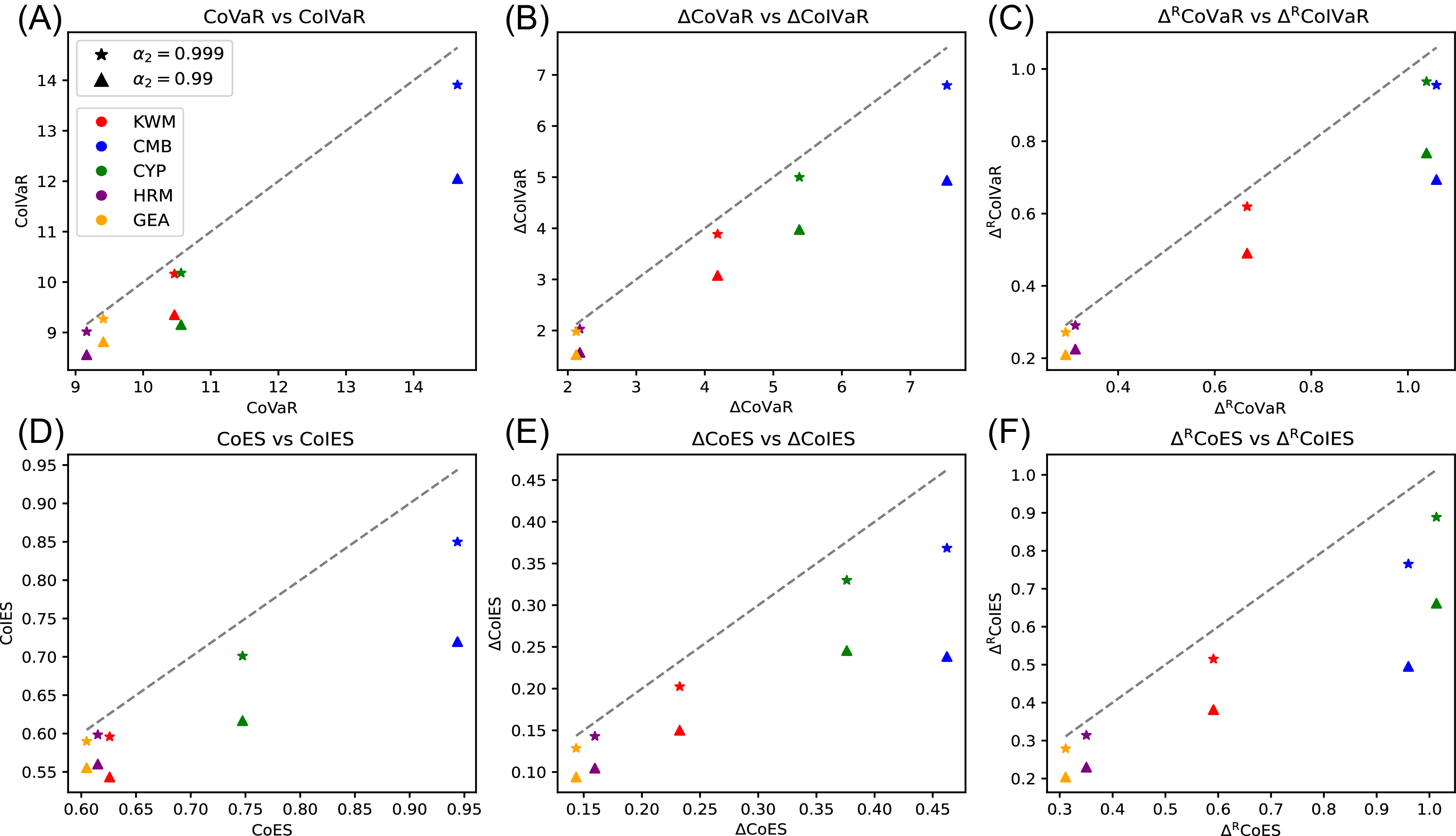
To further analyze the sensitivity of different assets to tail risk levels, we present scatter plots in Figure 7 to visually illustrate the relationships between various risk measures. The plots use the
 $ y = x $
diagonal as a reference, with different colors distinguishing stocks and different markers representing confidence levels.
Risk measures for
 $\alpha_1 = 0.95$
,
 $\alpha_2=0.999$
and
 $\beta = 0.95$
.

Scatter plot analysis based on different confidence levels and stocks.

The scatter plots present results consistent with the tabulated findings. CMB consistently exhibits higher risk levels, indicating its significant role in systemic risk assessment, while CYP shows more pronounced relative spillover effects. Additionally, data points fall below the
 $ y = x $
diagonal, suggesting that interval-based risk measures yield lower values than traditional risk measures. The scatter plots also reveal certain patterns that are not readily observable in the tables. When the confidence level
 $ \alpha_2 $
decreases, the reduction in systemic risk measures varies significantly across stocks. In absolute terms, CMB experiences the largest decline, indicating greater tail risk exposure – its potential losses escalate more rapidly in extreme market conditions. In relative terms, KWM, as measured by CoES (subfigure D), exhibits a relatively large tail risk exposure. After excluding extreme events, its risk level decreases significantly.
Risk measures for
 $\alpha_1 = 0.95$
,
 $\alpha_2=0.99$
and
 $\beta = 0.95$
.

5.3. Rolling-window estimation results
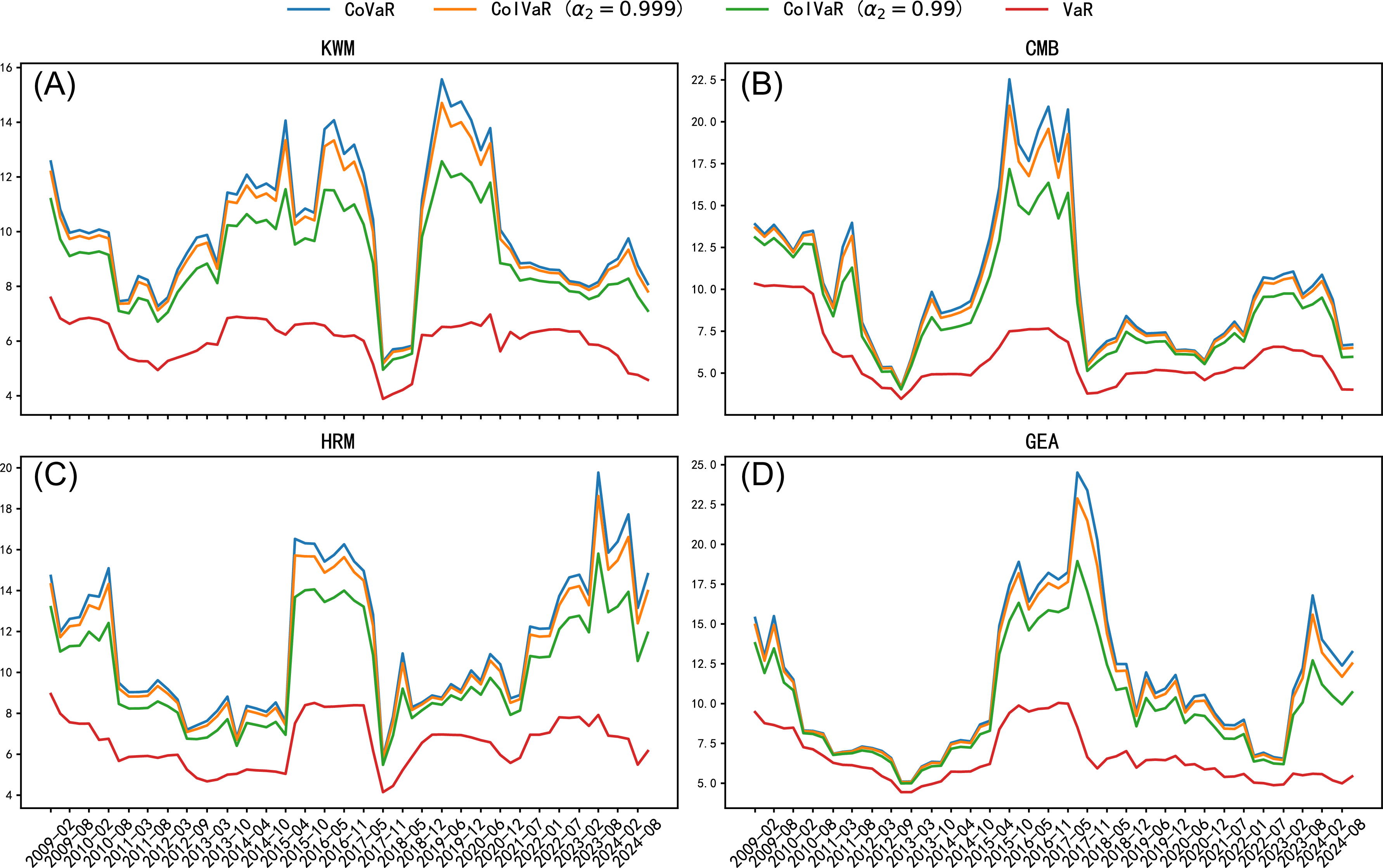
To provide a more comprehensive depiction of the dynamic characteristics of systemic risk, this study employs CoIVaR as a representative measure and applies a rolling-window approach for its computation. Specifically, the rolling window is set to two years (504 trading days) with a step size of one quarter (63 trading days). At each time point, model parameters are re-estimated based on the most recent data, yielding time-varying risk estimates. Figure 8 illustrates the evolution of systemic risk for four representative stocks–KWM, CMB, HRM, and GEA–under the fixed setting of
 $\alpha_1 = \beta = 0.95$
. The figure displays four types of risk measures: CoVaR, two versions of CoIVaR (with
 $\alpha_2 = 0.999$
and
 $\alpha_2 = 0.99$
), and VaR. This leads to the following findings.
Risk measures in rolling windows for different stocks.

-
(i) All conditional risk measures are consistently higher than the corresponding individual VaR, reflecting the positive correlation of risks in the stock market. Among the four selected stocks, CoVaR and CoIVaR exhibit highly consistent dynamic trends, whereas the VaR curve appears more independent. This suggests that individual VaR primarily captures idiosyncratic volatility, failing to effectively reflect external systemic risk transmission.
-
(ii) During periods of market stability or mild volatility, the numerical differences between CoVaR and CoIVaR remain relatively small. However, during episodes of heightened systemic risk – such as the 2015 stock market crash and the COVID-19 shock in 2020 – the discrepancy between the two measures widens significantly. This indicates that CoVaR is more sensitive to extreme systemic events, while CoIVaR offers greater estimation smoothness and robustness.
-
(iii) There are notable differences in how assets from different industries respond to systemic shocks. During stable market conditions, consumer and pharmaceutical stocks (e.g., KWM and HRM) still exhibit noticeable gaps between CoVaR and CoIVaR, indicating greater sensitivity to marginal systemic fluctuations. In contrast, financial and household appliance stocks (e.g., CMB and GEA) show near-identical values for both metrics over the same period, suggesting a more muted response to systemic volatility. This demonstrates CoIVaR’s ability to detect heterogeneous responses to systemic risk across industries before the system enters a fully stressed state, offering valuable insights into sectoral risk dynamics.
In summary, although CoVaR exhibits greater sensitivity under extreme systemic shocks – making it effective for identifying the most vulnerable nodes within the system – its reliance on tail observations can lead to heightened estimation volatility. In comparison, CoIVaR, by conditioning on a band of systemic states, not only captures risk transmission channels but also achieves superior smoothness and trend-tracking capability. It is thus better suited for routine macroprudential surveillance and systemic risk monitoring. Taken together, CoVaR and CoIVaR should be viewed as complementary tools, each offering distinct advantages in different policy and practical contexts.
6. Conclusions
Systemic risk refers to risks that affect the entire financial system or market, leading to widespread disruption, contagion, and spillover effects across interconnected entities. This paper introduces a novel framework for measuring systemic risk, with a particular focus on the spillover effects that arise from systemic risk and their implications for financial stability. We propose two advanced risk metrics: the CoIVaR and CoIES. These measures offer a more comprehensive approach to quantifying risk, incorporating interval-based uncertainty to capture the complexities of market dynamics under extreme conditions. Additionally, we introduce corresponding risk contribution measures that allow for the evaluation of the impact of individual assets or sectors on the overall systemic risk.
Through rigorous comparison of two sets of risk vectors under various stochastic orders and dependence structures, we validate the theoretical properties of the proposed risk measures. Numerical examples illustrate how these measures can be employed to evaluate the systemic risk exposure of different portfolios and sectors. Furthermore, the practical applicability of our framework is demonstrated by applying the proposed risk measures to stock market data, where our methodology is shown to effectively identify and measure spillover risks during periods of heightened market stress.
Future research could extend the framework developed in this paper in several directions. One potential area of exploration is the incorporation of machine learning techniques to improve the estimation and calibration of systemic risk measures, allowing for more adaptive and data-driven risk assessments. Another promising avenue is the development of dynamic models that capture the evolution of systemic risk over time, accounting for changing market conditions and the interplay between different risk factors. Additionally, extending the analysis to consider nonfinancial sectors, such as the real economy, could provide a more holistic view of systemic risk and its broader economic implications. Finally, exploring the use of the proposed risk measures in regulatory frameworks and their potential for improving risk-based capital requirements could contribute to more effective financial stability policies.
Supplementary material
The supplementary material for this article can be found at https://doi.org/10.1017/asb.2025.10077
Acknowledgements
This work was supported by the National Natural Science Foundation of China (No.72263019), Jiangxi Provincial Natural Science foundation (No. 20242BAB25017), and Graduate Innovation Fund Project of Jiangxi Provincial Department of Education (No. YC2024-B089).
Competing interests
No potential competing interest was reported by the author.
A. Proof of the main results
A.1. Proof of Lemma 4.2
Proof. Denote
 $Y_{h}=[Y|\mathrm{VaR}_{\alpha _{1}}[X]\lt X\leq \mathrm{VaR}_{\alpha_{2}}\left[ X\right] ]$
and let
 $Y_{h}\sim F_{Y_{h}}(y)$
. We can obtain
 \begin{eqnarray*}F_{Y_{h}}(y) &=&1-\mathbb{P}(Y\gt y|\mathrm{VaR}_{\alpha _{1}}[X]\lt X\leq \mathrm{VaR}_{\alpha _{2}}[X]) \\&=&1-\frac{\mathbb{P}\left( F(X)\gt \alpha _{1},G(Y)\gt G(y)\right) -\mathbb{P}\left( F(X)\gt \alpha _{2},G(Y)\gt G(y)\right) }{\alpha _{2}-\alpha _{1}} \\&=&1-\frac{\overline{C}\left( \alpha _{1},G(y)\right) -\overline{C}\left(\alpha _{2},G(y)\right) }{\alpha _{2}-\alpha _{1}} = 1-h_{\alpha _{1}-\alpha _{2}}\left( \overline{G}(y)\right) ,\end{eqnarray*}
where
 $h_{\alpha _{1}-\alpha _{2}}(t)=\frac{\overline{C}(\alpha _{1},1-t)-\overline{C}(\alpha _{2},1-t)}{\alpha _{2}-\alpha _{1}}$
, and satisfying
 $h_{\alpha _{1}-\alpha _{2}}(0)=0$
,
 $h_{\alpha _{1}-\alpha _{2}}(1)=1$
. According to
 $\partial_{v}^{2}C({\alpha_{1}},v)\leq \partial_{v}^{2}C({\alpha _{2}},v)$
, it can be shown that
 $\partial _{t}^{2}h_{\alpha _{1}-\alpha _{2}}(t)=\frac{\partial _{t}^{2}\overline{C}({\alpha _{1}},1-t)-\partial _{t}^{2}\overline{C}({\alpha _{2}},1-t)}{\alpha _{2}-\alpha _{1}}\leq 0.$
Hence,
 $h_{\alpha _{1}-\alpha _{2}}(t)$
is concave distortion function, and
 $Y_{h}$
is a distortion random variable derived from Y and
 $h_{\alpha_{1}-\alpha _{2}}(t)$
. This completes the proof.
A.2. Proof of Lemma 4.3
Proof. Denote
 $Y_h = [Y | \mathrm{VaR}_{\alpha_1}[X] \lt X \leq \mathrm{VaR}_{\alpha_2}[X]]$
and let
 $Y_h \sim F_{Y_h}(y)$
. It follows that
 $\mathrm{CoIVaR}_{\alpha _{1}-\alpha _{2},\beta }[Y|X] = F_{Y_{h}}^{-1}(\beta).$
By applying Lemma 4.2, it can be obtained that
 $F_{Y_h}(y)=1-h_{\alpha _{1}-\alpha _{2}}\left( \overline{G}(y)\right)$
, where
 $h_{\alpha_1-\alpha_2}(t) = \frac {\overline C(\alpha_1,1-t) - \overline C(\alpha_2,1-t)}{\alpha_2-\alpha_1}$
. Setting
 $F_{Y_h}(y) = \beta$
, we find
 $F_{Y_{h}}^{-1}(\beta) = G^{-1}\left(1-h^{-1}_{\alpha _{1}-\alpha _{2}}(1-\beta)\right) $
. This completes the proof.
A.3. Proof of Theorem 4.4
Proof. Using Lemma 4.2, it follows that
 \begin{align*}\mathrm{CoIVaR}_{\alpha _{1}-\alpha_{2},\beta }[Y|X]=G^{-1}\left(1-h^{-1}_{\alpha _{1}-\alpha _{2}}(1-\beta) \right)=G^{-1}\left(\overline h_{\alpha _{1}-\alpha _{2}}^{-1}(\beta )\right),\end{align*}
where
 $\overline h_{\alpha _{1}-\alpha _{2}}(t) = 1- h_{\alpha _{1}-\alpha _{2}}(1-t)=\frac{C(\alpha _{2},t)-C(\alpha _{1},t)}{\alpha _{2}-\alpha _{1}}$
. Similarly, we have
 \begin{align*}\mathrm{CoIVaR}_{\alpha _{1}-\alpha _{2},\beta }[Y^{\prime }|X^{\prime }] = G'^{-1}\left(1-h'^{-1}_{\alpha _{1}-\alpha _{2}}(1-\beta)\right) =G^{\prime -1}\left(\overline h_{{\alpha _{1}-\alpha _{2}}}^{\prime -1}(\beta )\right),\end{align*}
where
 $\overline h'_{\alpha _{1}-\alpha _{2}}(t) = 1- h'_{\alpha _{1}-\alpha _{2}}(1-t)=\frac{C'(\alpha _{2},t)-C'(\alpha _{1},t)}{\alpha _{2}-\alpha _{1}}$
.
Since
 $Y\leq _{\mathrm{SI[SD]}} Y^{\prime }$
, it follows that
 $G(y)\geq G^{\prime }(y)$
, or equivalently,
 $G^{-1}\left(\overline h_{{\alpha _{1}-\alpha_{2}}}^{-1}(\beta )\right)\leq G^{\prime -1}\left(\overline h_{{\alpha _{1}-\alpha _{2}}}^{-1}(\beta )\right)$
. Combining
 $\partial _{1}C(u,v) \geq \partial _{1}C^{\prime}(u,v)$
, we obtain
 $\overline h_{\alpha _{1}-\alpha _{2}}(t)\geq \overline h_{{\alpha _{1}-\alpha_{2}}}^{\prime }(t)$
, which implies
 $G^{\prime -1} \left(\overline h_{{\alpha _{1}-\alpha _{2}}}^{-1}(\beta ) \right)\leq G^{\prime -1}\left(\overline h_{\alpha _{1}-\alpha _{2}}^{\prime-1}(\beta )\right)$
. Therefore, the inequality (4.2) holds. This completes the proof.
A.4. Proof of Theorem 4.9
Proof. (i) According to the definition of CoIES and Lemma 4.3, it follows that
 $\mathrm{CoIES}_{\alpha_1 - \alpha_2,\beta}[Y|X] = \frac{1}{1- \beta} \int^1_\beta G^{-1}\left(\overline h_{\alpha _{1}-\alpha _{2}}^{-1}(t )\right) \mathrm{d}t,$
where
 $\overline h_{\alpha _{1}-\alpha _{2}}(t) =\frac{C(\alpha _{2},t)-C(\alpha _{1},t)}{\alpha _{2}-\alpha _{1}}$
. From the proof of Theorem 4.4, it is known that
 $Y \leq_{\mathrm{SI[SD]}} Y'$
and
 $\partial _1 C (u,v) \geq \partial_1 C' (u,v)$
imply
 $ G^{-1}\left(\overline h_{\alpha _{1}-\alpha _{2}}^{-1}(t )\right) \leq G'^{-1}\left(\overline h_{\alpha _{1}-\alpha _{2}}^{\prime -1}(t )\right) .$
Hence,
 \begin{equation*}\mathrm{CoIES}_{\alpha_1 - \alpha_2,\beta}[Y|X]\leq \mathrm{CoIES}_{\alpha_1 - \alpha_2,\beta}[Y'|X'].\end{equation*}
(ii) According to (i), the expression for
 $\mathrm{CoIES}_{\alpha_1 - \alpha_2,\beta}[Y|X]$
can be rewritten as
 \begin{equation*}\mathrm{CoIES}_{\alpha_1 - \alpha_2,\beta}[Y|X] = \frac{1}{1- \beta} \int^1_\beta G^{-1}\left(\overline h_{\alpha _{1}-\alpha _{2}}^{-1}(t )\right) \mathrm{d}t= \int^{1}_0 G^{-1} (s) \mathrm{d} A_{\alpha_1 - \alpha_2,\beta}(s),\end{equation*}
where
 \begin{equation} A_{\alpha _{1}-\alpha _{2},\beta }(s)=\begin{cases}0,&s\lt \overline h_{\alpha _{1}-\alpha _{2}}^{-1}(\beta) \\1-\frac{\overline{C}(\alpha _{1},s)-\overline{C}(\alpha _{2},s)}{(\alpha_{2}-\alpha _{1})(1-\beta )},&s {\geq}\overline h_{\alpha _{1}-\alpha _{2}}^{-1}(\beta )\end{cases}.\end{equation}
Similarly, we have
 \begin{equation*}\mathrm{CoIES}_{\alpha_1 - \alpha_2,\beta}[Y'|X'] = \frac{1}{1- \beta} \int^1_\beta G'^{-1}\left(\overline h_{\alpha _{1}-\alpha _{2}}'^{-1}(t )\right) \mathrm{d}t= \int^{1}_0 G'^{-1} (s) \mathrm{d} A'_{\alpha_1 - \alpha_2,\beta}(s),\end{equation*}
where
 \begin{equation} A_{\alpha _{1}-\alpha _{2},\beta }^{\prime }(s)=\begin{cases}0,&s\lt \overline h_{\alpha _{1}-\alpha _{2}}^{\prime -1}(\beta ) \\1-\frac{\overline{C}^{\prime }(\alpha _{1},s)-\overline{C}^{\prime }(\alpha_{2},s)}{(\alpha _{2}-\alpha _{1})(1-\beta )},&s {\geq} \overline h_{\alpha _{1}-\alpha _{2}}^{\prime -1}(\beta )\end{cases}.\end{equation}
According to
 $\partial^2_2 C({\alpha_1},v) \leq \partial^2_2 C({\alpha_2},v)$
and Lemma 4.8, when
 $s\gt \overline h_{\alpha _{1}-\alpha _{2}}^{-1}(\beta )$
,
 $A_{\alpha_1 -\alpha_2,\beta}(s)$
is a convex function of s. Then, for all
 $s \in(0,1)$
,
 $A_{\alpha_1 - \alpha_2,\beta}(s)$
is an increasing convex distortion function of s. From Lemma 4.8,
 $ Y \leq_{\mathrm{icx}} Y' $
implies
 \begin{equation} \int^{1}_0 G^{-1} (s) \mathrm{d} A_{\alpha_1 - \alpha_2,\beta}(s) \leq \int^{1}_0 G^{\prime -1} (s) \mathrm{d} A_{\alpha_1 - \alpha_2,\beta}(s).\end{equation}
Additionally, since
 $\partial _1 C (u,v) \geq \partial_1 C' (u,v)$
, it can be deduced that
 $A_{\alpha_1 - \alpha_2,\beta}(s) \geq A{'}_{\alpha_1 - \alpha_2,\beta}(s)$
, and it holds that
 $A_{\alpha_1 - \alpha_2,\beta}(0) = A{'}_{\alpha_1 - \alpha_2,\beta}(0) = 0$
,
 $A_{\alpha_1 - \alpha_2,\beta}(1) = A{'}_{\alpha_1 - \alpha_2,\beta}(1) = 1.$
Using integration by parts, the following inequality holds:
 \begin{equation} \int^{1}_0 G^{\prime -1}(s) \mathrm{d} A_{\alpha_1 - \alpha_2,\beta}(s)- \int^{1}_0 G^{\prime -1}(s) {\rm d} A'_{\alpha_1 - \alpha_2,\beta}(s) \leq 0.\end{equation}
From inequality (A3) and (A4), it can be shown that
 $\mathrm{CoIES}_{\alpha_1 - \alpha_2, \beta }[Y|X] \leq {\mathrm{CoIES}}_{\alpha_1 - \alpha_2, \beta}[Y'|X']$
holds. This completes the proof.
A.5. Proof of Theorem 4.13
Proof. Denote
 $Y_h = [Y |\mathrm{VaR}_{\alpha_1}[X] \lt X \leq {\mathrm{VaR}}_{\alpha_2}[X]]$
and
 $Y_h \sim F_{Y_h}(y)$
. According to Lemma 4.3, the
 $\rm \Delta CoIVaR$
is expressed as
 \begin{align*} \Delta {\mathrm{CoIVaR}}_{\alpha_1 - \alpha_2,\beta}[Y|X] = F_{Y_h}^{-1} (\beta) - G^{-1}(\beta) =G^{-1}\left(1- h_{\alpha _{1}-\alpha _{2}}^{-1}(1-\beta )\right) - G^{-1}(\beta),\end{align*}
where
 $ h_{\alpha _{1}-\alpha _{2}}(t) =\frac{\overline C(\alpha _{1},1-t)-\overline C(\alpha _{2},1-t)}{\alpha _{2}-\alpha _{1}}$
is a concave distortion function, given that
 $\partial^2_2 C(\alpha_1,v) \leq \partial^2_2 C(\alpha_2,v)$
, as stated in Lemma 4.2. Similarly,
 \begin{align*} \Delta {\mathrm{CoIVaR}}_{\alpha_1 - \alpha_2,\beta}[Y'|X'] = F_{Y'_h}^{-1} (\beta) - G'^{-1}(\beta) =G'^{-1}\left(1- h_{\alpha _{1}-\alpha _{2}}'^{-1}(1-\beta )\right) - G'^{-1}(\beta),\end{align*}
where
 $ h'_{\alpha _{1}-\alpha _{2}}(t) =\frac{\overline C'(\alpha _{2},1-t)-\overline C'(\alpha _{1},1-t)}{\alpha _{2}-\alpha _{1}}$
is a distortion function. From
 $\partial _1 C (u,v) \geq \partial_1 C' (u,v)$
, it follows that
 $h_{\alpha_1-\alpha_2}(t) \leq h_{\alpha_1-\alpha_2}'(t)$
. Combining
 $Y \leq_{\mathrm{disp} } Y'$
and Lemma 4.12, it can be deduced that
 \begin{equation*}F^{-1}_{Y_h}(\beta) - G^{-1}(\beta) \leq F^{-1}_{Y'_{h}}(\beta) - G'^{-1}(\beta).\end{equation*}
This completes the proof.
A.6. Proof of Theorem 4.15
Proof. Note that
 $\mathrm{ES}_\beta[Y] = \int^{1}_0 G^{-1} (s) \mathrm{d} H_{\beta}(s)$
, where
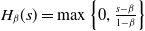 $H_{\beta}(s) = \max \left\{0, \frac{s-\beta}{1-\beta} \right\}$
. The
 $\rm \Delta CoIES$
is then expressed as
 \begin{equation*}\Delta \mathrm{CoIES}_{\alpha_1 - \alpha_2,\beta}[Y|X] = \int^{1}_0 G^{-1} (s) \mathrm{d} A_{\alpha_1 - \alpha_2,\beta}(s)-\int^{1}_0 G^{-1} (s) {\rm d} H_{\beta}(s),\end{equation*}
and similarly,
 \begin{equation*}\Delta \mathrm{CoIES}_{\alpha_1 - \alpha_2,\beta}[Y'|X'] = \int^{1}_0 G'^{-1} (s) {\rm d} A'_{\alpha_1 - \alpha_2,\beta}(s)-\int^{1}_0 G'^{-1} (s) {\rm d} H_{\beta}(s),\end{equation*}
where
 $A_{\alpha_1 - \alpha_2,\beta}(s)$
is defined in (A1) and
 $A'_{\alpha_1 - \alpha_2,\beta}(s)$
in (A2). Given
 $\partial^2_2 C(\alpha_1,v) \leq \partial^2_2 C(\alpha_2,v)$
, it follows that
 $A_{\alpha_1 - \alpha_2,\beta}(s)$
is a convex distortion function. Since
 $H^{-1}_\beta(t) = (1 - \beta)t + \beta$
is affine, the composite function
 $A_{\alpha_1 - \alpha_2,\beta}\left(H^{-1}_\beta(t)\right)$
is convex in t. According to Lemma 4.14,
 $Y \leq_{\mathrm{ew}} Y'$
implies
 \begin{equation*}\int^{1}_0 G^{-1} (s) \mathrm{d} A_{\alpha_1 - \alpha_2,\beta}(s) - \int^{1}_0 G^{-1} (s) \mathrm{d} H_{\beta}(s) \leq \int^{1}_0 G'^{-1} (s) \mathrm{d} A_{\alpha_1 - \alpha_2,\beta}(s) - \int^{1}_0 G'^{-1} (s) \mathrm{d} H_{\beta}(s).\end{equation*}
Since
 $\partial _1 C (u,v) \gt \partial_1 C' (u,v)$
, using integration by parts, it can be proved that
 \begin{equation*} \int^{1}_0 G'^{-1} (s) \mathrm{d} A_{\alpha_1 - \alpha_2,\beta}(s) - \int^{1}_0 G'^{-1} (s) \mathrm{d} A'_{\alpha_1 - \alpha_2,\beta}(s) = \int^{1}_0 \left(A'_{\alpha_1 - \alpha_2,\beta}(s)-A_{\alpha_1 - \alpha_2,\beta}(s)\right) \mathrm{d}G'^{-1} (s) \leq 0.\end{equation*}
Therefore, we have
 $\Delta \mathrm{CoIES}_{{\alpha _1} - {\alpha _2},\beta }[Y|X] \leq \mathrm{CoIES}_{{\alpha _1} - {\alpha _2},\beta }[Y'|X']$
. This completes the proof.
A.7. Proof of Theorem 4.17
Proof. (i) Denote
 $ Y_{h,\alpha} = [Y \mid \mathrm{VaR}_{\alpha}[X] \lt X \leq \mathrm{VaR}_{\alpha_2}[X]] $
and
 $ Y'_{h,\alpha} = [Y' \mid \mathrm{ VaR}_{\alpha}[X'] \lt X' \leq {\mathrm{VaR}}_{\alpha_2}[X']] $
, with
 $ \alpha \in \{\alpha_1, 1/2\} $
, and let
 $ Y_{h,\alpha} \sim F_{Y_{h,\alpha}},\; Y'_{h,\alpha} \sim F_{Y'_{h,\alpha}} $
. Then,
 \begin{align*}\Delta^{\mathrm{med}}\mathrm{CoIVaR}_{\alpha_1 - \alpha_2, \beta}[Y|X]= G^{-1}\big(1 - h_{\alpha_1 - \alpha_2}^{-1}(1 - \beta)\big)- G^{-1}\big(1 - h_{1/2 - \alpha_2}^{-1}(1 - \beta)\big),\end{align*}
 \begin{equation*}\Delta ^{\mathrm{med}}\mathrm{CoIVaR}_{\alpha _{1}-\alpha _{2},\beta }\left[Y^{\prime }|X^{\prime }\right] =G^{\prime -1}\left( 1-h_{\alpha _{1}-\alpha_{2}}^{\prime -1}(1-\beta )\right) -G^{\prime -1}\left( 1-h_{1/2-\alpha_{2}}^{\prime -1}(1-\beta )\right) ,\end{equation*}
where
 \begin{align*}h_{\alpha - \alpha_2}(t) = \frac{\overline{C}(\alpha, 1 - t) - \overline{C}(\alpha_2, 1 - t)}{\alpha_2 - \alpha}, \quad h'_{\alpha - \alpha_2}(t) = \frac{\overline{C}'(\alpha, 1 - t) - \overline{C}'(\alpha_2, 1 - t)}{\alpha_2 - \alpha}.\end{align*}
Combining
 $Y \leq_{\mathrm{disp}} Y'$
and Lemma 4.12, when
 $1-h^{-1}_{1/2-\alpha_2}(1-\beta) \leq 1-h^{-1}_{\alpha_1-\alpha_2}(1-\beta)$
, it suffices to show that (4.5). Next, it is necessary to prove that
 $h_{\alpha-\alpha_2}(t)$
is increasing in
 $\alpha$
. Let
 $U=F(x)$
and
 $V=G(y)$
, and suppose
 $Y \uparrow_{\mathrm{RTI}} X$
, we have
 $\mathbb P(Y\gt y|X\gt x)$
increasing in x, which implies
 \begin{equation*} \mathbb P(V\gt v|U\gt u)=\frac{\overline{C}(u,v)}{1-u}\end{equation*}
is increasing in u. Hence, it follows that
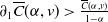 $\partial_1 \overline{C}(\alpha,v)\gt \frac{\overline{C}(\alpha,v)}{1-\alpha}$
. For
 $\alpha \lt \alpha_2$
, the condition
 $\frac{\overline{C}(\alpha,v)}{1-\alpha} \lt \frac{\overline{C}(\alpha_2,v)}{1-\alpha_2}$
holds if and only if
 $\frac{\overline{C}(\alpha,v)}{1-\alpha} \cdot \frac{1-\alpha_2}{\alpha_2-\alpha} \lt \frac{\overline{C}(\alpha_2,v)}{1-\alpha_2} \cdot\frac{1-\alpha_2}{\alpha_2-\alpha}$
, which further implies
 \begin{align*}\frac{\overline{C}(\alpha ,v)}{1-\alpha }\cdot \left( \frac{1-\alpha }{\alpha _{2}-\alpha }-1\right) \lt \frac{\overline{C}(\alpha _{2},v)}{\alpha_{2}-\alpha },\end{align*}
leading to
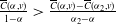 $\frac{\overline{C}(\alpha,v)}{1-\alpha} \gt \frac{\overline{C}(\alpha,v) - \overline C(\alpha_2,v)}{\alpha_2-\alpha}$
. Hence,
 $\partial_1 \overline{C}(\alpha,v) \gt \frac{\overline{C}(\alpha,v) - \overline C(\alpha_2,v)}{\alpha_2-\alpha}$
, which proves that
 $h_\alpha(1-t)$
is increasing in
 $\alpha$
. This completes the proof.
(ii) From the proof of Theorem 4.9, the
 $\rm \Delta^{med} CoIES$
is expressed as
 $\Delta^{med} {CoIES}_{\alpha_1 - \alpha_2,\beta}[Y|X] = \int^{1}_0 G^{-1} (s) \mathrm{d} A_{\alpha_1 - \alpha_2,\beta}(s)-\int^{1}_0 G^{-1} (s) \mathrm{d} A_{1/2 - \alpha_2,\beta}(s),$
where
 \begin{equation} A_{\alpha -\alpha _{2},\beta }(s)=\begin{cases}0,&s\lt \overline h_{\alpha-\alpha _{2}}^{-1}(\beta) \\1-\frac{\overline{C}(\alpha,s)-\overline{C}(\alpha _{2},s)}{(\alpha_{2}-\alpha )(1-\beta )},&s {\geq} \overline h_{\alpha -\alpha _{2}}^{-1}(\beta )\end{cases},\quad \alpha \in \{\alpha_1,1/2\}.\end{equation}
Similarly,
 $\Delta^{med} {CoIES}_{\alpha_1 - \alpha_2,\beta}[Y'|X'] = \int^{1}_0 G'^{-1} (s) {\mathrm d} A'_{\alpha_1 - \alpha_2,\beta}(s)-\int^{1}_0 G'^{-1} (s) {\mathrm d} A'_{1/2 - \alpha_2,\beta}(s),$
where
 \begin{equation} A'_{\alpha -\alpha _{2},\beta }(s)=\begin{cases}0,&s\lt \overline h_{\alpha-\alpha _{2}}'^{-1}(\beta) \\1-\frac{\overline{C}'(\alpha,s)-\overline{C}'(\alpha _{2},s)}{(\alpha_{2}-\alpha )(1-\beta )},&s {\geq} \overline h_{\alpha -\alpha _{2}}'^{-1}(\beta )\end{cases},\quad \alpha \in \{\alpha_1,1/2\}.\end{equation}
According to Lemma 4.14, t is necessary to prove that the continuous function
 $A_{\alpha - \alpha_2,\beta} \left(A^{-1}_{1/2 - \alpha_2,\beta}(s)\right)$
is convex, which is equivalent to showing that
 $(A_{\alpha_1 - \alpha_2,\beta}(s))'/(A_{1/2 - \alpha_2,\beta}(s))'$
is increasing in s. Here,
 $(A_{\alpha - \alpha_2,\beta}(s))'$
is given by
 $$(A_{\alpha - \alpha_2,\beta}(s))'= \frac{\partial A_{\alpha - \alpha_2,\beta}(s)}{\partial s} = \begin{cases} 0,&s\lt \overline h_{\alpha-\alpha _{2}}^{-1}(\beta) \\\frac{\mathbb P(\alpha \lt U \leq \alpha_2|V=s)}{(1-\beta)(\alpha_2-\alpha)},& s {\geq} \overline h_{\alpha-\alpha _{2}}^{-1}(\beta) \end{cases}.$$
Since g(x,y) is
 $\mathrm{TP}_2$
, it follows that
 $g(x_1,y_1)g(x_2,y_2) \geq g(x_1,y_2)g(x_2,y_1)$
for all
 $x_1 \leq x_2$
and
 $y_1 \leq y_2$
. This implies that
 $ \frac{\mathbb P(\alpha_1 \lt U \leq \alpha_2|V=s)}{\mathbb P(1/2 \lt U \leq \alpha_2|V=s)}$
is increasing in s, that is,
 ${A^{'}_{\alpha_1 - \alpha_2,\beta}(s)}/{A^{'}_{1/2 - \alpha_2,\beta}(s)}$
is increasing in s. Therefore,
 $A_{\alpha - \alpha_2,\beta} (A^{-1}_{1/2 - \alpha_2,\beta}(s))$
is convex function, and
 $Y \leq_{\mathrm{ew}} Y'$
implies (4.6). This completes the proof.
A.8. Proof of Theorem 4.19
Proof. (i) According to Lemma 4.3, we have
 \begin{align*}\Delta^{\mathrm{R}} \mathrm{CoIVaR}_{\alpha_1 - \alpha_2, \beta}[Y|X] = \frac{G^{-1}\left( \overline h^{-1}_{\alpha_1 - \alpha_2}(\beta) \right)}{G^{-1}(\beta)} - 1, \quad\Delta^{\mathrm{R}} \mathrm{CoIVaR}_{\alpha_1 - \alpha_2, \beta}[Y'|X'] = \frac{G'^{-1}\left( \overline h'^{-1}_{\alpha_1 - \alpha_2}(\beta) \right)}{G'^{-1}(\beta)} - 1,\end{align*}
where
 \begin{align*}\overline h_{\alpha_1 - \alpha_2}(t) = \frac{C(\alpha_2, t) - C(\alpha_1, t)}{\alpha_2 - \alpha_1}, \quad\overline h'_{\alpha_1 - \alpha_2}(t) = \frac{C'(\alpha_2, t) - C'(\alpha_1, t)}{\alpha_2 - \alpha_1}.\end{align*}
Since
 $ \partial^2_2 C(\alpha_1, v) \leq \partial^2_2 C(\alpha_2, v) $
, the function
 $ \overline h_{\alpha_1 - \alpha_2}(t) $
is convex, implying
 $t \leq \overline h^{-1}_{\alpha_1 - \alpha_2}(t).$
Moreover, under
 $ Y \leq_* Y' $
, it follows that
 \begin{align*}\frac{G^{-1}(\overline h^{-1}_{\alpha_1 - \alpha_2}(\beta))}{G^{-1}(\beta)} \leq \frac{G'^{-1}(\overline h^{-1}_{\alpha_1 - \alpha_2}(\beta))}{G'^{-1}(\beta)}.\end{align*}
In addition,
 $ \partial_1 C(u,v) \geq \partial_1 C'(u,v) $
implies
 $ \overline h_{\alpha_1 - \alpha_2}(t) \geq \overline h'_{\alpha_1 - \alpha_2}(t) $
, hence
 \begin{align*}\frac{G'^{-1}(\overline h^{-1}_{\alpha_1 - \alpha_2}(t))}{G'^{-1}(t)} \leq \frac{G'^{-1}(\overline h'^{-1}_{\alpha_1 - \alpha_2}(t))}{G'^{-1}(t)}.\end{align*}
Combining the above, we conclude (4.8).
(ii) Note that
 \begin{align*}\Delta^{\mathrm{R}} \mathrm{CoIES}_{\alpha_1 - \alpha_2, \beta}[Y|X] = \frac{\int_0^1\! G^{-1}(s)\, \mathrm{d}A_{\alpha_1 - \alpha_2,\beta}(s)}{\int_0^1 G^{-1}(s)\, \mathrm{d}H_\beta(s)} - 1, \quad\!\!\Delta^{\mathrm{R}} \mathrm{CoIES}_{\alpha_1 - \alpha_2, \beta}[Y'|X'] = \frac{\int_0^1\! G'^{-1}(s)\, \mathrm{d}A'_{\alpha_1 - \alpha_2,\beta}(s)}{\int_0^1 G'^{-1}(s)\, \mathrm{d}H_\beta(s)} - 1,\end{align*}
where
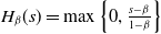 $H_\beta(s) = \max\left\{0, \frac{s - \beta}{1 - \beta} \right\}$
, and
 $A_{\alpha_1 - \alpha_2,\beta}$
,
 $A'_{\alpha_1 - \alpha_2,\beta}$
are defined in (A1) and (A2), respectively. By Theorem 4.15, the condition
 $ \partial_2^2 C(\alpha_1, v) \leq \partial_2^2 C(\alpha_2, v) $
implies that
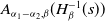 $ A_{\alpha_1 - \alpha_2,\beta}(H_\beta^{-1}(s)) $
is convex in s. Then, applying Lemma 4.18, we obtain
 \begin{align*}\frac{\int_0^1 G^{-1}(t)\, \mathrm{d}A_{\alpha_1 - \alpha_2,\beta}(t)}{\int_0^1 G^{-1}(t)\, \mathrm{d}H_\beta(t)} \leq \frac{\int_0^1 G'^{-1}(t)\, \mathrm{ d}A_{\alpha_1 - \alpha_2,\beta}(t)}{\int_0^1 G'^{-1}(t)\, \mathrm{d}H_\beta(t)}.\end{align*}
Since
 $ \partial_1 C(u,v) \geq \partial_1 C'(u,v) $
, using integration by parts, it can be proved that
 \begin{align*}\int_0^1 G'^{-1}(t)\, \mathrm{d}A_{\alpha_1 - \alpha_2,\beta}(t) \leq \int_0^1 G'^{-1}(t)\, \mathrm{d}A'_{\alpha_1 - \alpha_2,\beta}(t).\end{align*}
Combining the above yields (4.9), which completes the proof.
A.9. Proof of Theorem 4.21
Proof. Note that
 $\Delta^{\mathrm{R-med}} \mathrm{CoIVaR}_{{\alpha _1} - {\alpha _2},\beta }[Y|X] = \frac{G^{-1}\left(1-h^{-1}_{\alpha_1-\alpha_2}(1-\beta)\right)} { G^{-1}\left(1-h^{-1}_{1/2-\alpha_2}(1-\beta)\right)} -1,$
and
 $\Delta^{\mathrm{R-med}} \mathrm{CoIVaR}_{{\alpha _1} - {\alpha _2},\beta }[Y'|X'] = \frac{G'^{-1}\left(1-h^{-1}_{\alpha_1-\alpha_2}(1-\beta)\right)} { G'^{-1}\left(1-h^{-1}_{1/2-\alpha_2}(1-\beta)\right)}-1,$
where
 $h_{\alpha-\alpha_2}(t) =\frac{\overline C(\alpha,1-t) - \overline C (\alpha_2,1-t)}{\alpha_2-\alpha} $
, with
 $\alpha \in \{\alpha_1,1/2\}$
. According to Theorem 4.17, if
 $Y \uparrow_{\mathrm{RTI}} X$
, it follows that
 $h^{-1}_{1/2-\alpha_2}(t) \geq h^{-1}_{\alpha_1-\alpha_2}(t)$
. By combining
 $Y \leq_{*} Y'$
, the desired result is obtained.
(ii) Note that
 $ \Delta^{\mathrm{R-med}} \mathrm{CoIES}_{{\alpha _1} - {\alpha _2},\beta }[Y|X] = \frac{\int_0^1 G^{-1}(s) \mathrm{d} A_{\alpha_1-\alpha_2}(s)}{\int_0^1 G^{-1}(s) \mathrm{d} A_{1/2-\alpha_2}(s)} -1,$
and
 $ \Delta^{\mathrm{R-med}} \mathrm{CoIES}_{{\alpha _1} - {\alpha _2},\beta }[Y'|X'] = \frac{\int_0^1 G'^{-1}(s) \mathrm{d} A_{\alpha_1-\alpha_2}(s)}{\int_0^1 G'^{-1}(s) \mathrm{d} A_{1/2-\alpha_2}(s)} -1,$
where
 $A_{\alpha - \alpha_2,\beta}(s)$
is defined in (A5). According to Theorem 4.17, when
 $g(x,y) = \mathbb P(x\lt X\leq x'|Y=y)$
is
 $\mathrm{TP}_2$
,
 $A_{\alpha_1 - \alpha_2,\beta}\left(A^{-1}_{1/2 - \alpha_2,\beta}(s)\right)$
is convex function in s. By combining
 $Y \leq_{\mathrm{ps}} Y'$
and Lemma 4.18, the desired result is obtained. This completes the proof.