


1. Introduction
With the advancement of intelligent manufacturing and agricultural automation, agricultural production is gradually moving toward intelligence and precision to address the challenges of food security brought by global population growth and the increasing cost of agricultural labor [Reference Zhao, Wei and Gan1]. The integration of robotics and precision agriculture is of great significance for improving the utilization rate of agricultural resources and reducing production costs, which has become an important development trend of modern agriculture [Reference Höffmann, Patel and Büskens2]. At present, autonomous agricultural robots are widely applied in field operations, including autonomous mowing [Reference Höffmann, Patel and Büskens2–Reference Xie, Liu, Wang, Liu, Wang, Li and Yang5], crop protection [Reference Faiçal, Freitas, Gomes, Mano, Pessin, de Carvalho, Krishnamachari and Ueyama6, Reference Tan, Huang, Tang, Fang and Huang7], fertilization [Reference Mier, Valente and de Bruin8, Reference Mier, Faulí, Valente and de Bruin9], and sowing [Reference Vahdanjoo, Gislum and Sørensen10]. These operations typically require robots to completely cover the target field without omission while performing specific tasks such as spraying, fertilizing, or seeding.
To achieve reliable field operations, coverage path planning (CPP) is a fundamental technology for autonomous robots. It aims to generate complete paths that ensure full coverage of farmland without redundancy. Compared with traditional robotics, agricultural coverage involves larger operational areas and higher repeatability, which imposes stricter requirements on planning efficiency and path quality. Therefore, efficient CPP is essential for improving the operational performance of agricultural robots.
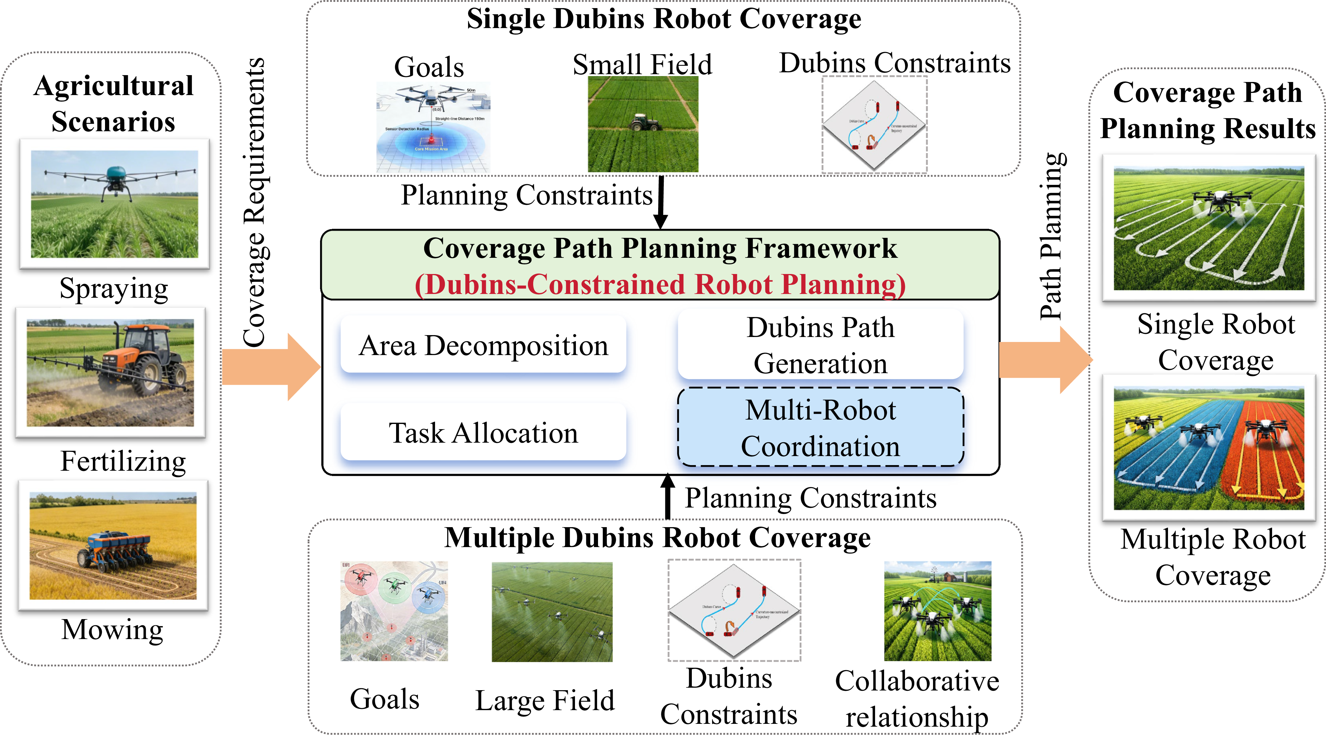
Area coverage path planning for Dubins robots.

Figure 1. Long description
A diagram illustrating the coverage path planning framework for Dubins-constrained robot planning in agricultural scenarios. Panel A: Agricultural Scenarios. This section shows images of agricultural tasks such as spraying, fertilizing, and mowing. Panel B: Single Dubins Robot Coverage. This section includes goals, small field coverage, and Dubins constraints. Panel C: Coverage Path Planning Framework. This section outlines the framework with components like area decomposition, task allocation, Dubins path generation, and multi-robot coordination. Panel D: Multiple Dubins Robot Coverage. This section includes goals, large field coverage, Dubins constraints, and collaborative relationships. Panel E: Coverage Path Planning Results. This section shows the results of path planning for single robot coverage and multiple robot coverage.
Extensive studies have focused on CPP for single agricultural robots. However, limitations in operation range, battery capacity, and computational resources make it difficult for a single robot to handle large-scale tasks. In contrast, multi-robot systems offer higher efficiency and better robustness [Reference Chen, Du, Zhang, Han and Wei11–Reference Sharma and Voruganti13]. As a result, multi-robot coverage path planning (MCPP) has attracted increasing attention in recent years. To reflect the state-of-the-art in MCPP, recent studies can be broadly categorized into online planning for unknown or dynamic environments and offline planning for known environments. For uncertain unknown environments, methods such as EA-OSPGB [Reference Cai, Zhang, Xin, Peng and Wang14] enable online coordination through energy-based strategies, while OARP-Replan [Reference Ramesh, Imeson, Fidan and Smith15] focuses on real-time replanning under time constraints. For known and static environments, such as structured farmland, research mainly focuses on improving global efficiency and resolving multi-robot conflicts. For example, large scale multi-robot coverage path planning (LS-MCPP) [Reference Tang, Mao and Ma16] combines spanning tree coverage with local search to optimize completion time.
However, despite these recent advancements, most existing studies still assume that the robots have omnidirectional steering capability or only abstractly penalize turning costs, thereby neglecting strict nonholonomic kinematic constraints such as the minimum turning radius. Nevertheless, in agricultural applications such as fixed-wing UAVs and autonomous agricultural vehicles, which are often subject to nonholonomic kinematic constraints, including minimum turning radius. If these constraints are ignored during the planning stage, the generated path may contain sharp turns, which would force the robot to make frequent adjustments, thereby reducing efficiency. As illustrated in Figure 1, an effective MCPP framework must simultaneously handle multiple constraints. The planning framework takes different scenario requirements as input and invokes the corresponding algorithm to generate coverage paths for the robot. Both single-robot algorithm and multi-robot algorithm need to satisfy a series of planning constraints (such as task goals, region scale, and the Dubins constraints), while the multi-robot algorithm needs to further consider the collaborative relationship among multiple robots.
As a typical nonholonomic kinematic model, the Dubins robot model is constrained by the minimum turning radius. Many agricultural robots such as fixed-wing UAVs and autonomous agricultural vehicles can be modeled in this way. Compared with the omnidirectional robot model, imposing Dubins kinematic constraints aligns more closely with the practical motion features of agricultural robots. This not only helps generate smooth paths with high executability but also enables a more accurate assessment of operating costs of the coverage path, thereby facilitating the estimation of energy consumption and coverage time. Therefore, this study focuses on multi-robot coverage under Dubins kinematic constraints and aims to develop an efficient planning method for agricultural applications.
Some reviews have summarized various approaches to solving MCPP problems [Reference Tan, Mohd-Mokhtar and Arshad17–Reference Abujabal, Fareh, Sinan, Baziyad and Bettayeb19]. These methods can be classified into two categories: exact and heuristic. Although the proposed MCPP methods have good performance, they still face some challenges in agricultural scenarios. Specifically, the exact MCPP method searches the entire solution space to find the optimal solution [Reference Li, Shi, Jin, Yang, Zhou, Lian and Liu20]. However, in the large-scale farmland environment, the solution space scale expands rapidly, resulting in an exponential increase in computing time, and it is difficult to apply to the real-time operation requirements of large-scale farmland. In contrast, heuristic methods usually adopt clustering and other strategies to improve computational efficiency [Reference Tang, Mao and Ma16, Reference Chen, Zhang, Wu, You and Ning21], which are more suitable for large-scale farmland coverage tasks. However, such methods compress the search space, which may reduce the accuracy of solutions.
To address these challenges mentioned above, this study focuses on the CPP of multiple Dubins robots in agricultural environments. We will integrate the practical needs in agricultural scenarios, comprehensively considering factors such as farmland geometry (convex or non-convex), kinematic constraints of the robots, and the scale of the multi-robot system. It aims to propose an efficient method that satisfies the kinematic constraints of agricultural robots while reducing the coverage time and improving the operational efficiency. The main contributions of this study are as follows:
-
• We formulate the multi-robot CPP problem for Dubins vehicles in farmland scenarios as an exact optimization model. Inspired by the Generalized Traveling Salesman Problem (GTSP) problem, we encapsulate the decomposed rectangular sub-regions as “atomic coverage tasks” with a fixed Dubins traversal pattern. This design ensures complete coverage of each sub-region without introducing additional endpoint continuity constraints. By performing an exhaustive search within the solution space, the exact model guarantees the theoretically optimal coverage path.
-
• We propose a multi-robot cooperative CPP method based on game theory for large-scale environments. To minimize the maximum completion time, this method introduces a game-theoretic task negotiation mechanism. It dynamically optimizes task reallocation among robots based on actual Dubins path costs. Consequently, the method accurately reflects true workload variations and achieves an optimal balance between computational efficiency and operational load balancing.
-
• The effectiveness of the proposed framework is validated through extensive comparative experiments and high-fidelity simulations. Experimental results demonstrate that our method provides significant advantages in both workload balancing and overall coverage time. Furthermore, simulations on a high-fidelity fixed-wing UAV platform verify that the generated paths strictly satisfy practical flight constraints, proving the practicality of the method for real-world farmland applications.
The remaining part of this article is as follows: Section 2 describes the related work on the area CPP problem. Section 3 provides a detailed definition of the problem and the exact mathematical model based on Dubins robots. Section 4 elaborates on the design of the heuristic algorithm game-based Dubins multi-robot coverage path planning algorithm (GDM). Section 5 conducts a detailed experiment on the proposed algorithm. Section 6 summarizes the content of the entire article.
2. Related work
2.1. Curvature-constrained and unconstrained MCPP
Robot kinematic constraints are key factors that determine the efficiency and feasibility of CPP [Reference Šelek, Seder, Brezak and Petrović22]. Among those, the curvature constraint, as an important factor in robot planning, has a direct impact on the operational efficiency and feasibility of agricultural robots. Based on the curvature constraint, agricultural robots can be classified into two categories: curvature-constrained robots and curvature-unconstrained robots. Curvature-unconstrained robots are typically represented by differential drive robots, which have the ability to turn in place and are suitable for working in small fields. In contrast, curvature-constrained robots (e.g., Dubins robots) are unable to achieve lateral movement, and their trajectories are strictly limited to a specific direction (e.g., forward or backward), which is suitable for a large farmland environment. Robots with curvature constraints cannot include sharp turns in the planned paths, which increases the complexity of the planning process. Based on the above differences in the curvature constraint of robots, MCPP methods can be categorized into curvature-constrained MCPP and curvature-unconstrained MCPP accordingly [Reference Wang, Jiang, Li and Sun23].
Several methods have been proposed to solve the curvature-unconstrained MCPP problem. Based on their ability to provide an optimal solution, these methods can be classified into two categories: exact algorithms and heuristic algorithms. Exact algorithms typically utilize mixed-integer linear programing [Reference Chen, Du, Zhang, Han and Wei11, Reference Zhou, Wang, Ding, Hu and Shang24], dynamic programing, and other strategies to model the MCPP as a rigorous optimization problem. In contrast, heuristic algorithms often represent the target area as graph or tree structures [Reference Gao and Xin25–Reference Tang, Sun and Zhang28] and employ strategies such as clustering [Reference Xiao, Li, Xie, Ni, Zhang and Wang12], depth-first search [Reference Li, Shi, Jin, Yang, Zhou, Lian and Liu20], or vehicle routing problem formulations [Reference Kapoutsis, Chatzichristofis and Kosmatopoulos26] to generate approximately balanced coverage areas.
Recent advancements in these heuristic frameworks have predominantly focused on high-level optimization to improve operational efficiency. For instance, researchers have proposed efficient frameworks for large-scale grid coverage [Reference Tang, Mao and Ma16], anytime replanning strategies for dynamic environments [Reference Ramesh, Imeson, Fidan and Smith15], and energy-aware algorithms for multi-robot teams [Reference Cai, Zhang, Xin, Peng and Wang14]. Although these methods effectively minimize makespan and balance workloads, they primarily operate at the high-level decision-making layer, often treating turns as heuristic penalties or neglecting kinematic feasibility. As a result, the generated paths may contain sharp turns that violate the minimum turning radius required by practical agricultural machinery. This limitation is also evident in more application-driven frameworks. For example, Zhang et al. [Reference Zhang, Zhang, Zhang, Gao, Feng and Yue29] proposed a vehicle–UAV collaborative coverage approach for large-scale environments, but it relies on simplified 2D Euclidean distance models that do not explicitly account for the kinematic constraints of ground vehicles.
Aiming at the real-world coverage requirements, a series of MCPP methods for curvature-constrained robots has been proposed. Several methods initially generated preliminary paths without considering the turning radius constraint, and subsequently smoothed the turning points to satisfy the robot kinematic constraints. For example, Hoffmann et al. [Reference Höffmann, Patel and Büskens30] proposed a NURBS-based method to generate smooth headland paths. And then they developed a full-coverage method [Reference Höffmann, Patel and Büskens2] for agricultural vehicles, which utilized Dubins curves to smooth sharp turns to ensure the kinematic feasibility of planned paths. Similarly, Yu et al. [Reference Yu, Fan, Cui, Xia and Wang31] first generated paths using a simulated annealing-whale optimization algorithm and then smoothed the sharp turns with NURBS curves to meet kinematic constraints. Gkesoulis et al. [Reference Gkesoulis, Georgakis, Karras and Bechlioulis32] employed the A* algorithm to compute the shortest collision-free path between two points. Then a controller was used to monitor the robot’s motion state and dynamically adjust parameters like velocity to ensure smooth turning. Selek et al. [Reference Šelek, Seder, Brezak and Petrović22] proposed the smooth complete coverage path planning (SCCPP) method, which generates initial paths based on the spanning tree algorithm and utilizes the clothoids of the cyclotron curve [Reference Brezak and Petrović33] to smooth the initial path. Similarly, Choton and Prabhakar [Reference Choton and Prabhakar3] proposed an optimal multi-robot coverage method (OM), which divides the farmland into multiple small areas, then improves coverage efficiency by calculating the optimal coverage direction within each subdivided area and employs Dubins curves to smooth turning points. However, OM is only applicable to the convex polygonal farmland areas. Mier et al. [Reference Mier, Valente and de Bruin8] initially proposed an open-source solution called Fields2Cover for CPP of Dubins agricultural vehicles. However, this solution could only handle convex farmland areas. Therefore, in their subsequent work [Reference Mier, Faulí, Valente and de Bruin9], they expanded Fields2Cover to make it applicable to non-convex areas and took capacity constraints into account for the planning. Agarwal and Akella [Reference Agarwal and Akella34] introduced a deviation tolerance to optimize the motion smoothness of robots during sharp turns. Within the allowable deviation range, the robot can temporarily deviate from the path segments to be covered. However, this strategy comes at the cost of compromising path coverage integrity, resulting in certain segments being left uncovered, which is not acceptable in certain situations, such as spraying pesticides.
Although existing methods provide strong foundations, they predominantly follow a “plan-first, smooth-later” paradigm. Such decoupling fails to capture the explicit impact of continuous curvature constraints on turning costs during the search process, often leading to sub-optimal solutions. To address this limitation, some studies attempt to consider turning maneuvers during the planning stage. However, these methods do not explicitly model turning costs within a kinematic framework. Yang et al. [Reference Yang, Du, Zhang, Wang, Zhang and Wu35] incorporate turning patterns and penalties into the optimization but enforce curvature constraints only in post-processing. Zhang et al. [Reference Zhang, Li, Wang, Jin and Wang36] introduce a direction-consistency criterion into an A* framework, where directional changes are penalized during the search. Xie et al. [Reference Xie, Liu, Wang, Liu, Wang, Li and Yang5] reduce high-cost maneuvers by optimizing operation sequences and favoring efficient turning patterns while avoiding costly ones such as reversing. Despite these efforts, these methods mainly reduce the number or types of turning maneuvers rather than explicitly modeling turning costs under continuous curvature constraints. As a result, kinematic feasibility is not fully integrated into the planning process, and cost evaluation remains loosely coupled with motion constraints. This may still lead to sub-optimal or infeasible trajectories.
To address this limitation, recent studies incorporate Dubins curves directly into path generation. This approach enables more accurate cost evaluation. For example, Karapetyan et al. [Reference Karapetyan, Moulton, Lewis, Li, O’Kane and Rekleitis37] proposed two heuristic algorithms, DCAC and DCRC, for large-scale environments. The DCAC algorithm partitions an undirected weighted graph via spatial clustering for single-robot routing. Meanwhile, the DCRC algorithm decomposes a global Hamiltonian loop into multiple sub-paths. To further improve multi-robot coordination, Tan et al. [Reference Tan, Huang, Tang, Fang and Huang7] introduced a multi-elite strategy to avoid local optima. Similarly, Li et al. [Reference Li, Zhou, Jin, Chen, Man and Shi4] considered variable-speed scenarios to minimize fleet size under deadline constraints. Additionally, Li et al. [Reference Li, Shi, Jin, Yang, Zhou, Lian and Liu20] developed two CPP methods for multiple Dubins robots. The first is an exact optimization algorithm (EDM), which computes the shortest feasible Dubins path between points [Reference Dubins38] and then applies mixed integer linear programing to obtain the optimal solution. The second is a heuristic algorithm (CDM), which divides the target area into sub-areas using tree partition and plans coverage paths for each robot. However, both methods have clear limitations. EDM relies on a centralized mathematical model. It yields theoretical optimality but suffers from poor scalability. On the other hand, CDM employs rigid geometric partitioning, which often causes severe workload imbalances. To overcome these challenges, this article proposes the GDM framework. We introduce a path-cost-aware mechanism to dynamically redistribute tasks. Instead of using simple geometric areas, GDM relies on actual Dubins path costs for task redistribution. This approach accurately reflects the true workload variations among robots. This strategy breaks the conventional limitation that a “balanced area guarantees balanced coverage time.” Consequently, GDM achieves an optimal trade-off between computational efficiency and operational load balancing.
In summary, a large number of excellent works have been developed and can be applied to the CPP for curvature-unconstrained robots. However, these methods have obvious deficiencies when dealing with the path planning for curvature-constrained robots. While the traditional method of “planning first, smoothing later” is workable, the cost of turning is usually high. If this factor is disregarded during the planning step, it will lead to a large gap between the estimated and real path costs. Therefore, integrating the Dubins constraints directly into the planning stage is a better choice. At the same time, how to balance the calculation accuracy and efficiency remains a challenge that needs to be addressed in this field.
2.2. Game theory and multi-robot task allocation
As a key problem in multi-robot systems, task allocation has been widely used in the fields of coordinated perception [Reference Queralta, Taipalmaa, Pullinen, Sarker, Gia, Tenhunen, Gabbouj, Raitoharju and Westerlund39], UAV formation [Reference Niu, Liu, Lin and Du40], task scheduling [Reference Amador, Okamoto and Zivan41] and area coverage [Reference Höffmann, Patel and Büskens18, Reference Ramos, Pinto and Haddad42]. Excellent task allocation results can significantly improve the performance and robustness of the system. In recent years, a variety of task allocation methods have been proposed [Reference Khamis, Hussein and Elmogy43]. For example, methods based on market [Reference Dias, Zlot, Kalra and Stentz44], auction [Reference Choi, Brunet and How45] and game [Reference Garapati, Roldán, Garzón, del Cerro and Barrientos46–Reference Roldán, Cerro and Barrientos48]. Among them, the game-based task allocation method, which leverages cooperation and competition among robots to optimize decision-making, has gained significant attention.
Game theory is a mathematical analysis method to explore how individuals make decisions in an environment where competition and cooperation coexist [Reference Owen49]. In general, game theory involves basic elements such as players, strategy sets, and a utility function. The players refer to the decision-making subjects involved in the game. The strategy set denotes the collection of actions available to each player. The utility function measures a player’s preference for the outcome of the game. From the perspective of whether players cooperate or not, games can be classified into two categories: cooperative games and noncooperative games [Reference Li, Wu and Chen50]. Cooperative games refer to the situation where players can reach an optimal strategy jointly through negotiation and cooperation. Players will form a coalition to achieve maximum collective welfare, so it is also known as a coalitional game. Noncooperative games are those in which players do not reach a strong agreement but make decisions based on their individual interests.
Cooperation among robots not only improves efficiency but also enhances the robustness of the system. For the MCPP problem, all robots share the same objective, which is to minimize the maximum coverage time. Therefore, robots can establish cooperative alliances and negotiate task reallocation to optimize task assignments. For example, some works [Reference Luan, Xu, Liu, Du, Qian, Liu and Tong47, Reference Li, Wu and Chen50, Reference Jin, Tang, Chen and Peng51] introduce methods that enable robots to establish cooperative coalitions for task allocation, with experiments that verify its effectiveness in improving task efficiency. In addition, other researchers [Reference Garapati, Roldán, Garzón, del Cerro and Barrientos46, Reference Roldán, Cerro and Barrientos48] examined the cooperative and competitive behaviors of UAV swarms in task performance, introducing algorithms based on both diagrams. The work ultimately concluded that cooperation provides significant advantages in terms of task success rates.
In summary, game-based task allocation methods have shown good performance in the field of multi-robot coordination. However, most existing methods suit specific application domains and lack solutions for MCPP involving robots with curvature constraints. Therefore, this study proposes a game-based MCPP method that leverages path coordination through balanced area division, optimizing both the maximum coverage time and the balance of load.
3. Problem description and mathematical modeling
3.1. Problem statement
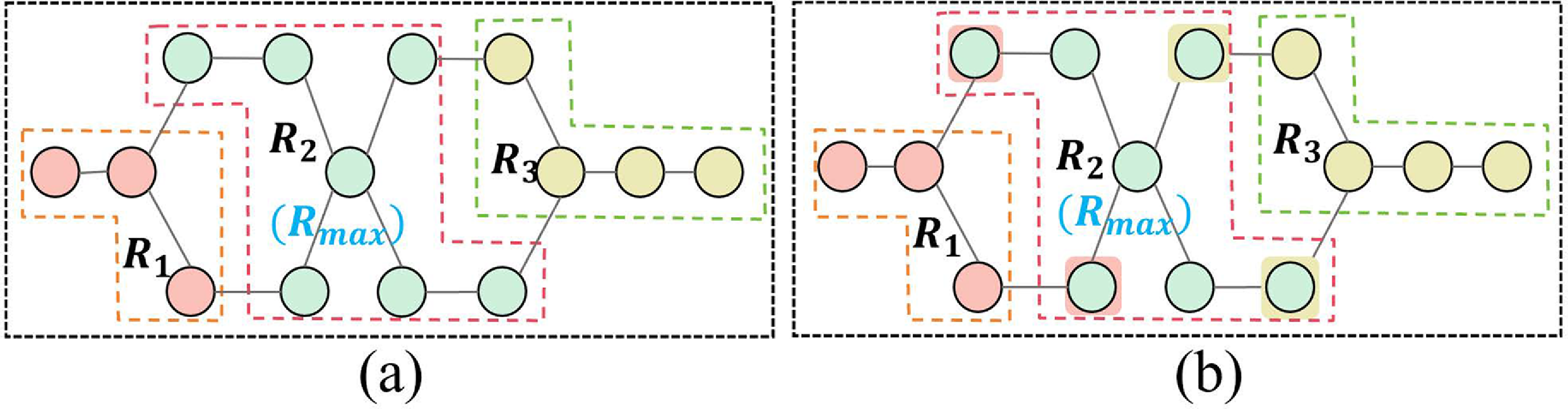
Examples of target area and decomposition. 1-Headland areas. 2-Main working area. 3-Obstacle.

The target area
 $A$
is a two-dimensional field area with known boundaries and obstacles (as illustrated in Figure 2(a)). In this study, to ensure full coverage and accommodate the turning requirements of nonholonomic robots, the area
 $A$
is categorized into two functional zones: the Main Working Area, denoted as
 $A_{main}$
, and the Headland Areas, denoted as
 $A_{head}$
, located at the boundaries of the field and obstacles (as illustrated in Figure 2(b)).
Due to the presence of obstacles,
 $A_{main}$
is typically a non-convex polygon. We employ the Boustrophedon decomposition method [Reference Lewis, Edwards, Benson, Rekleitis and O’Kane52] to decompose the
 $A_{main}$
into
 $M$
rectangular cells (Figure 2(c)). These
 $M$
rectangular cells form the set
 $T = \{t_1, t_2, \ldots , t_M\}$
. The width of each rectangular cell is equal to the sensor width of the robot. As shown in Figure 2(d), each rectangular cell is represented by its upper and lower endpoints and the connecting line. The length of each cell is defined to fully span the vertical extent of
 $A_{main}$
. Robots will cover a rectangular cell by moving vertically along the connecting line in a top-to-bottom or bottom-to-top pattern.
Crucially, the Dubins curves for transitioning between cells are executed within
 $A_{head}$
. Therefore, the robot ensures that the
 $A_{main}$
is 100% covered by the effective sensor width. Any potential coverage gaps caused by the minimum turning radius are confined to the
 $A_{head}$
, which is typically pre-covered by boundary-following passes in practical agricultural operations.
We utilize
 $N$
homogeneous Dubins robots to cover the target area
 $A$
. These
 $N$
homogeneous Dubins robots represent the set of robots
 $RN=\{R_1,R_2,\ldots ,R_N\}$
. All robots in
 $RN$
are equipped with the same sensors that cover the square grid of side length
 $r_1$
. All robots start from the same starting point
 $sp$
. After the coverage task is completed, all robots must return to the starting point
 $sp$
.
Definition: The CPP problem for multiple Dubins robots can be described as: plan
 $N$
paths for
 $N$
homogeneous Dubins robots. These paths must start from the same common starting point, traverse all rectangular cells exactly once, and return to the starting point. The optimization objective is to minimize the coverage time of the longest path while satisfying the minimum turning radius constraint of robots.
3.2. Mathematical modeling
This study proposes an exact mathematical model to obtain optimal coverage paths for multiple Dubins robots, aiming to minimize the maximum coverage time. The optimal coverage paths should satisfy the following constraints:
 $(C1)$
Each rectangular cell must be covered exactly once;
 $(C2)$
All paths must start from the starting point and return to the starting point.
 $(C3)$
The path between the endpoints must satisfy the curvature constraint.
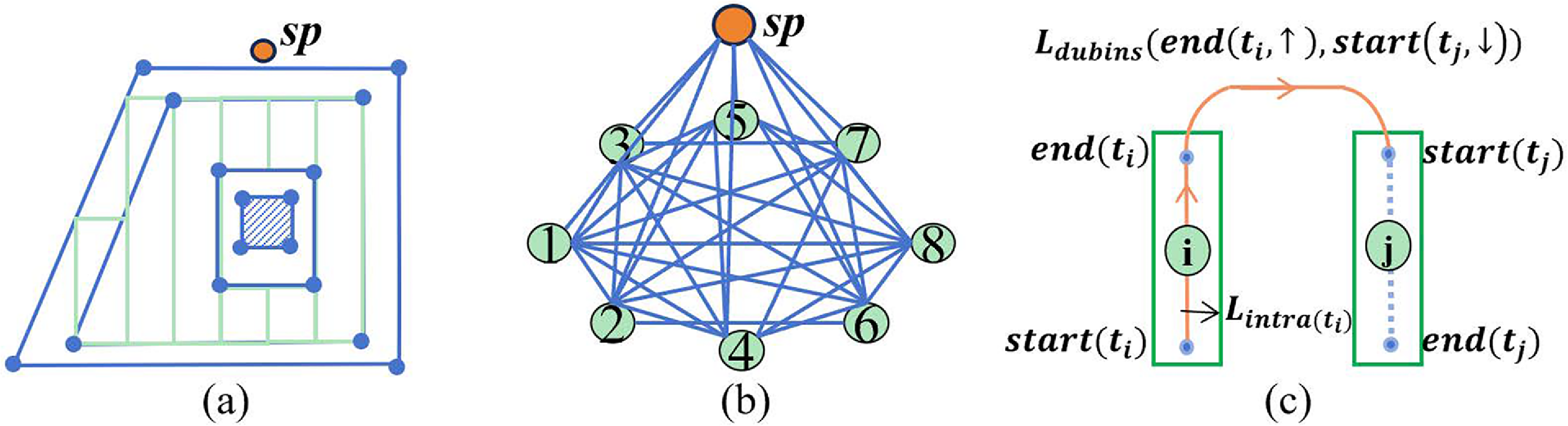
A key constraint for rectangular cells is that once the robot reaches any endpoint of a cell, it must completely cover the entire rectangular area corresponding to that endpoint. Traditional exact methods typically construct a model based on all endpoints of rectangular cells and rely on the adjacency between endpoints to ensure complete coverage of the rectangular cells [Reference Li, Shi, Jin, Yang, Zhou, Lian and Liu20]. However, this method may encounter situations where the endpoints are accessed but the rectangular cells are not covered during the solution process, thereby reducing the solution efficiency. Therefore, inspired by the GTSP problem, we encapsulate the decomposed rectangular cells as “atomic coverage tasks” with a fixed Dubins traversal pattern, ensuring complete coverage of the cells without the need to introduce additional endpoint continuity constraints. Meanwhile, to satisfy the kinematic constraints of robotic motion, we connect these nodes using Dubins paths. As shown in Figure 3(b), all edges between nodes in the graph are Dubins curves [Reference Dubins38]. In other words, the distance between any two nodes is defined as the length of the shortest Dubins path connecting these two points, which satisfies the constraint
 $(C3)$
. The details are as follows:
Dubins path cost model for coverage graph.

The MCPP problem is modeled as a graph traversal problem. As shown in Figure 3(b), the field area is represented as an undirected graph
 $G_0 = \{V_0, E_0\}$
, where
 $V_0 = T \cup \{sp\}$
is composed of all rectangular cells and the starting point
 $sp$
. The edge set
 $E_0$
consists of the connections between any two nodes in
 $V_0$
. The goal is to traverse all vertices in the graph exactly once, while the starting point
 $sp$
can be visited multiple times.
First, each rectangular cell can be covered in two opposite directions. Therefore, for any cell
 $t \in T$
, we define a set of coverage modes
 $A_c = \{\uparrow , \downarrow \}$
, where
 $\uparrow$
and
 $\downarrow$
denote covering the cell from one endpoint to the other in opposite directions. An atomic coverage task is defined as a pair
 $ ( t, a)$
, where
 $t \in T$
and
 $a \in A_c$
. Executing task
 $(t, a)$
means that the robot enters the coverage cell
 $t$
in the mode
 $a$
, completes the full coverage of the cell, and exits from the corresponding endpoint. Thus, the set of atomic coverage tasks can be defined as:
 \begin{equation} \text{SET} = \{(t, a) \mid t \in T, a \in A_c\} \end{equation}
Suppose that the coverage path of the
 $n$
-th robot is
 $P_n=\{g_{n,1},g_{n,2}, \dots , g_{n, K_n}\}$
, where
 $g_ {n, 1 }= g_{n, K_n} = sp$
,
 $g_ {n, 2} ,\ldots , g_{n,K_n-1} \in SET$
. The order of elements in the path represents the sequence in which the robot performs atomic coverage tasks. For any two consecutive atomic coverage tasks
 $g_i = (t_i, a_i)$
and
 $g_j = (t_j, a_j)$
, where
 $t_i \neq t_j$
, the cost of transitioning from task
 $g_i$
to task
 $g_j$
is defined as:
 \begin{equation} C(g_i, g_j) = L_{\text{intra}}(t_i) + L_{\text{dubins}}(\text{end}(t_i, a_i), \text{start}(t_j, a_j)),t_i \neq t_j \end{equation}
Here,
 $L_{\text{intra}}(t_i)$
represents the internal coverage time cost of the cell
 $t_i$
, which is calculated by the path length divided by the robot’s working speed. Similarly,
 $L_{\text{Dubins}}(.)$
represents the transition time cost, which is determined by the shortest Dubins path between the exit of task
 $g_i$
and the entrance of task
 $g_j$
. Since the Dubins path inherently accounts for the curvature constraints,
 $L_{\text{Dubins}}$
effectively incorporates the time penalty associated with turning maneuvers. Figure 3(c) illustrates the cost calculation from task
 $g_i = (t_i, \uparrow )$
to task
 $g_j = (t_j, \downarrow )$
.
Suppose
 $f(P_n)$
represents the time cost of the path
 $P_n$
, then the total cost of the coverage paths for the
 $n$
-th robot is defined as:
 \begin{equation} f\left ( P_{n} \right ) = \sum _{l=1}^{K_{n}-1} C(g_{n,l},\; g_{n,l+1}). \end{equation}
Based on the aforementioned variables and definitions, the exact mathematical model for the multi-robot Dubins CPP problem can be formulated as follows:
 \begin{equation} \min (\!\max \{ f(P_1 ), \dots , f(P_N ) \}) \end{equation}
s.t.
 \begin{equation} P_1\cup P_2 \cup \dots \cup P_N=SET\cup \{sp\} \end{equation}
 \begin{equation} P_i\cap P_j=\{sp\},i\neq j,1\leq i,j\leq N \end{equation}
 \begin{equation} \left | \left \{ (t, a) \in P_1 \cup \cdots \cup P_N \right \} \right | = 1,\forall t \in T \end{equation}
Eq. (5) ensures that all coverage tasks in the set
 $SET$
will be performed by the robots. Eq. (6) guarantees that each coverage task is visited by only one robot, avoiding redundant coverage. Eq. (7) ensures that each cell is fully covered. Eqs. (5)−(7) ensures that each rectangular cell is covered exactly once, while all paths start from the starting point
 $sp$
, corresponding to the constraints
 $(C1)$
and
 $(C2)$
.
Although the exact model can obtain the optimal solution, the MCPP problem is NP-hard [Reference Li, Zhou, Jin, Chen, Man and Shi4]. As the computational scale increases, the computation time grows explosively, making it difficult to be applied to large-scale environments. Therefore, developing heuristic methods is an effective way to solve large-scale MCPP problems. In the next section, we will propose a heuristic algorithm based on game theory to solve the MCPP problem of multiple Dubins robots.
4. Game-based Dubins Multi-robot coverage algorithm
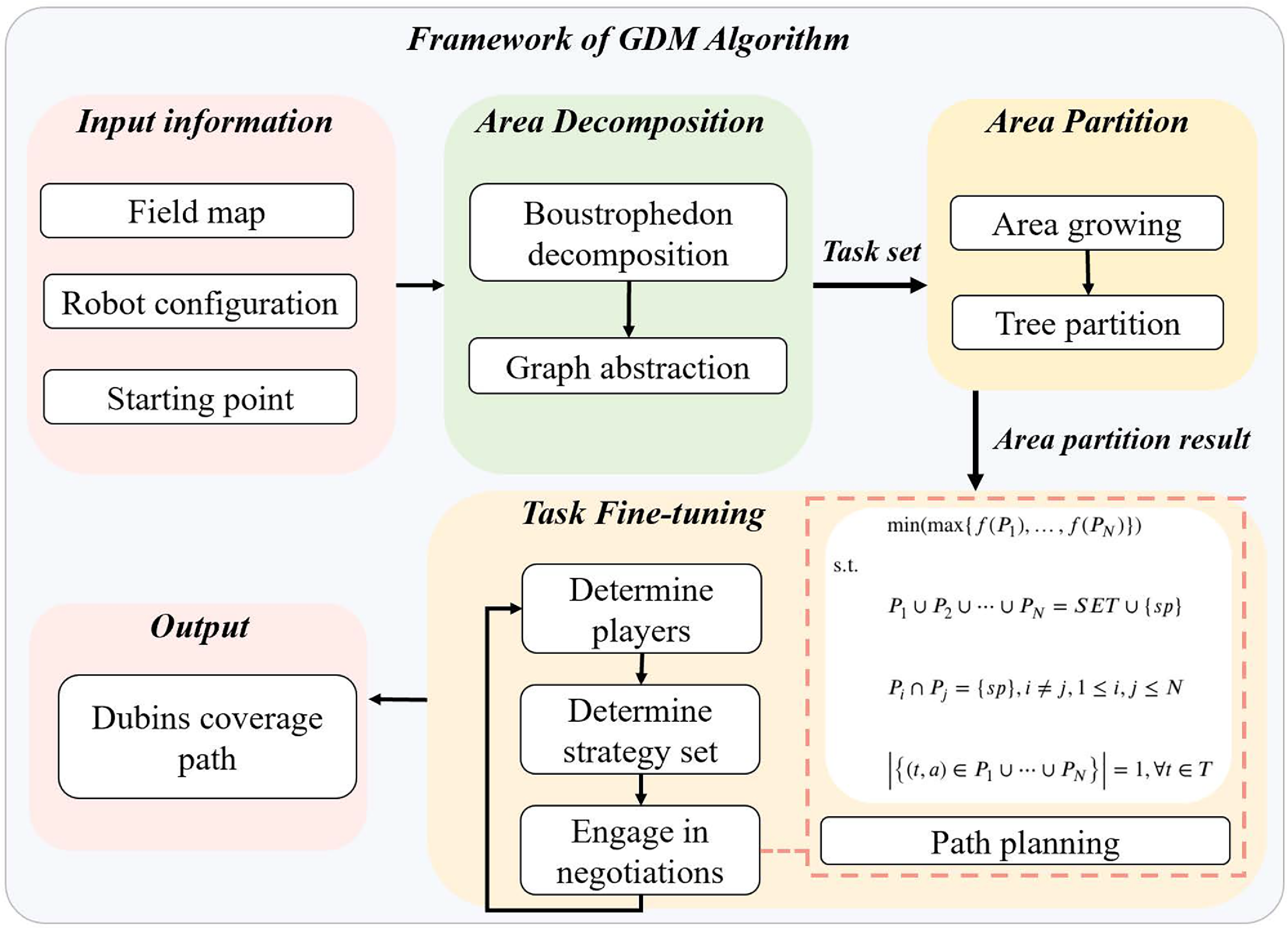
We propose a novel GDM to address the MCPP problem. As shown in Figure 4, the GDM receives the field map, starting point, robot configuration, and finally outputs the Dubins coverage paths. GDM consists of three components, i.e., area decomposition, area partition, and task fine-tuning. The area decomposition component divides the target area
A
into rectangular cells. The area partition component divides all cells into
 $N$
subsets, while the task fine-tuning component further improves the quality of task assignment by the game-based negotiation strategy and generates the Dubins coverage path for each robot.
4.1. Area decomposition component
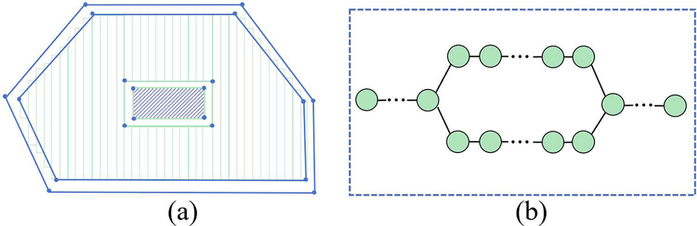
As shown in Figure 5(a), the area decomposition component decomposes the field area into
 $M$
rectangular cells using boustrophedon decomposition [Reference Lewis, Edwards, Benson, Rekleitis and O’Kane52]. These
 $M$
rectangular cells form the set
 $T = \{t_1, t_2, \dots , t_M\}$
. Subsequently, all cells in
 $T$
are abstracted as an undirected graph
 $G = (V, E)$
, where
 $V$
represents nodes corresponding to the rectangular cells (Figure 5(b)). Each node is assigned a weight equal to the size of the rectangular cell. The edges in the set
 $E$
are established between nodes if their corresponding cells are adjacent. It should be noted that the graph
 $G$
in this case is different from the graph
 $G_0$
used in the exact method. In graph
 $G$
, edges only exist between adjacent vertices.
GDM algorithm framework.

Figure 4. Long description
A framework diagram of the GDM algorithm for multi-robot coordination and path planning. The diagram is divided into several sections: Input information, Area Decomposition, Area Partition, Task Fine-tuning, and Output. Input information includes Field map, Robot configuration, and Starting point. Area Decomposition involves Boustrophedon decomposition and Graph abstraction. Area Partition includes Area growing and Tree partition. Task Fine-tuning consists of Determine players, Determine strategy set, Engage in negotiations, and Path planning. The Output is the Dubins coverage path. The diagram illustrates the flow from input information through area decomposition and partition, task fine-tuning, to the final output.
Area decomposition and graph abstraction.

4.2. Area partition component
The area partition component aims to partition the set
 $T$
into
 $N$
subsets by an area growing strategy. Each subset corresponds to a continuous area and is covered by a single robot. The core idea of the area growing strategy is as follows: The cells in
 $T$
are ordered, progressing from left to right and from bottom to top.
 $N$
cells are selected at equal intervals to serve as the initial cells (Figure 6(a)). Next, the unassigned cells adjacent to these initial cells are gradually merged (Figure 6(b)). Each merge updates the weights of the corresponding subsets. This process continues until all cells have been allocated, ensuring a fair distribution of cells among all subsets (Figure 6(c)).
After merging, the area growing strategy can generate an initial task assignment result (Figure 6(c)). However, due to the starting point of the robot and obstacle locations, the initial partition results may be unbalanced. Therefore, the task allocation module adopts the tree partition strategy [Reference Li, Shi, Jin, Yang, Zhou, Lian and Liu20] to further improve the balance of task assignment (Figure 6(d)).
Example of area partition process.

4.3. Task fine-tuning component
The area partition component aims to provide a balanced area partition result. However, the balanced area partition result is not equivalent to the balanced coverage path. Therefore, the task fine-tuning component adopts a strategy based on game theory, which allows part of the robots to negotiate task reallocation to generate coverage paths with the shortest time cost while satisfying the kinematic constraints of Dubins robots.
The task fine-tuning component based on game strategy performs rounds of negotiation. Each negotiation involves three steps: determining the robots to play the game, determining the task set to be negotiated, and engaging in negotiations by rules. The task reallocation problem is formulated as a game, which can be represented as a quadruple
 $\left ( \mathbf{P}_r, \mathbf{S}_r, \mathbf{U}_r, \mathbf{C}_s \right )$
.
-
•
 $\mathbf{P}_r$
represents the set of game players, which is a subset of
$RN$
that forms a coalition aimed to minimize the maximum coverage time.
-
•
$\mathbf{S}_r$
represents the strategy set. It is the set of strategies from which the coalition can choose. Players will select a certain strategy to maximize the coalition’s welfare. In this problem, robots achieve the optimization goal by reallocating task cells, so the strategy set is composed of the units that robots can allocate. The specific details are explained in the following sections. -
•
$\mathbf{U}_r$
represents the utility function. This value measures the preference of a player for a task, where a higher value indicates a stronger preference of the robot for a certain task. The calculation method for each player is given by Eqs. (8) and (9). -
•
$\mathbf{C}_s$
represents the characteristic function. The characteristic function describes the collective welfare of the coalition. The goal of all players is to maximize the collective welfare or minimize the collective cost. These two values are determined by the longest coverage path, where an increase in collective welfare represents a reduction in the collective cost (maximum coverage time). The formal definition is provided in Eq. (10).


The task fine-tuning process is accomplished by multiple rounds of games. In each round of games, robots form a coalition to negotiate, and they compute a new task allocation scheme that can shorten the maximum coverage time and reassign it. When the negotiation is successful, the maximum coverage time is reduced. After multiple rounds of games, the maximum coverage time gradually approaches the optimal value.
4.3.1. Utility function and characteristic function
In game theory, players make decisions based on the utility function and the characteristic function. For players, they will choose strategies with higher utility function values while satisfying the requirements of the characteristic function, which is to increase collective welfare. In this study, it is assumed that all players are rational, meaning that in the coalition, players will agree to the outcome of the game if collective welfare increases. In the MCPP problem, the coverage time is the cost of the robot. The shorter the coverage time, the greater the welfare. Therefore, the objective of the coalition is to minimize the maximum coverage time. We assume that the robots’ speeds are fixed, so the utility function and characteristic function can be directly measured by the length of the coverage path.
The cost of a robot is defined as
 $cost$
, where
 $cost(TS (R_Q))$
represents the time cost of the
 $R_Q$
’s coverage path, which can be solved with a single-robot path planning solver [Reference Helsgaun53]. For a specific task
 $t_i$
, the utility provided to the robot
 $R_Q$
should be evaluated. This is usually divided into two cases: assigning
 $t_i$
away from robot
 $R_Q$
, and assigning
 $t_i$
to robot
 $R_Q$
by another robot. Therefore, the utility of task
 $t_i$
to robot
 $R_Q$
can be defined in two forms:
 \begin{equation} U_ {R_Q ,t _i} ^ {Remove} = cost (TS(R_Q)) - cost (TS(R_Q)/t_i ) \end{equation}
which
 $cost(TS (R_Q)/t_i)$
represents the cost of the robot
 $R_Q$
after removing task
 $ t_i$
from the set of tasks of
 $R_Q$
.
 \begin{equation} U_ {R_Q ,t _i} ^{ Add} = cost (TS(R_Q)) - cost (TS(R_Q) \cup t_i ) \end{equation}
which
 $cost(TS (R_Q) \cup t_i)$
represents the cost of the robot
 $R_Q$
after adding task
 $t_i$
to the task set of
 $R_Q$
.
Furthermore, the characteristic function is defined as
 $C_s$
, which represents the change in the maximum cost of the coverage time. Assuming that the current system cost is
 $cost(R_{max})$
, and upon task reallocation, it is updated to
 $cost(R_{max}^{'})$
, then
 $C_s$
can be described as:
 \begin{equation} C_s=cost(TS(R_{max}))-cost(TS(R_{max}^{'})) \end{equation}
In a round of a game, a positive value of the characteristic function means a reduction in the maximum coverage time cost, thereby enhancing collective welfare. Consequently, only when the value of the characteristic function remains positive will all players accept the outcome of the game.
4.3.2. Determine players
To improve computational efficiency, only two robots would be selected in each round of the game. The robot with the current maximum cost
 $R_{max}$
and one of its neighboring robots are chosen as players in the game. Among all neighboring robots in adjacent areas, the one with the lowest cost has a higher probability of successful negotiation due to the larger load gap with
 $R_{max}$
. Therefore, the robot with the minimum cost is selected first from all neighborhoods as the other party in the game. Through task negotiation and allocation between them, the maximum time cost can be reduced. If the robot with the current minimum cost fails to reach an agreement with
 $ R_{\text{max}}$
, then the next robot with the second lowest cost is selected as the other party in the game until a successful negotiation is reached or there are no more optional neighboring robots.
In addition, the cost of robot
 $R_n$
is denoted as
 $Cost(TS(R_n))$
. This cost is defined as the total execution time to complete the task sequence. It is calculated based on the total length of the coverage path
 $P_n$
and the operating speed of the robot. This calculation is performed using a single-robot solver [Reference Helsgaun53]. The path
 $P_n$
explicitly includes both straight segments and Dubins turning transitions. By considering Dubins kinematics,
 $Cost(TS(R_n))$
inherently and accurately captures the actual time consumption of turning maneuvers. At the same time, the current coverage path
 $P_n$
of the robot can be obtained. Let
 $R_{max}$
denote the robot with the maximum completion time. As shown in Figure 7, the game is defined between
 $R_{max}$
(player 1) and a neighboring robot
 $R_{j}\in N(R_{max})$
(player 2), where
 $N(R_{max})$
represents the neighboring set of
 $R_{max}$
.
Example of players and strategy set.

4.3.3. Determine the strategy set
A strategy set in game theory represents a collection of optional strategies available to players. As mentioned above, the robot
 $R_{max}$
with the maximum coverage time is set as one of the players. By allocating some cells of
 $R_{max}$
to other robots, the cost of
 $R_{max}$
could be reduced. Considering the equilibrium and non-intersection requirements of MCPP, if
 $R_{j}$
represents the negotiating counterpart, the strategy set
 $S_r$
must be constructed from the task cells located at the boundary within
 $R_{max}$
that are adjacent to
 $R_{j}$
. The allocation of these cells is determined through predefined negotiation rules. Figure 7 illustrates an example of determining the strategy set. Formally, the strategy set is defined as follows:
 \begin{equation} S_r = \left \{ t \mid t \in TS(R_{\max }) \land \left ( \exists t' \in TS(R_{j}),\ (t, t') \in E \right ) \right \} \end{equation}
4.3.4. Negotiation rules
The game process is essentially the process of negotiation among players. We assume that all players are rational and share a common goal: reducing the maximum coverage time cost will lead to an acceptable outcome for all players. This makes a unique case where during the mutual negotiations between two robots, if they successfully lower the maximum coverage time, even at the expense of increasing another robot’s coverage time, the result is still accepted. This aligns with our objective of narrowing the coverage time gap between robots and achieving a more balanced distribution.
During negotiations,
 $R_{max}$
that takes the longest coverage time will negotiate with another player
 $R_{j}$
until a better task allocation strategy is achieved. Assuming that the current task to be negotiated is
 $t_0$
, each negotiation round involves robots calculating their utility functions and characteristic functions to access whether the proposed task reallocation meets the optimization objective. The robots must follow the following rules:
-
• When
$U_ {R_Q ,t _i} ^ {Remove} \leq 0$
, it follows that
$C_s\leq 0$
. This indicates that offloading task
$t_0$
results in an increase in the maximum coverage time, leading to a failed negotiation. -
• When
$ U_{R_Q,t_i}^{\text{Remove}} \gt 0$
, and if
$ U_{R_Q,t_i}^{\text{Add}} \geq 0$
, it follows that
$ U_s \gt 0$
. This indicates that offloading the task
$ t_0$
to
$ R_{j}$
reduces costs for both parties and results in a decrease for the maximum coverage time, thus achieving a successful negotiation. -
• When
$U_ {R_Q ,t _i} ^ {Remove} \gt 0$
and
$U_ {R_Q ,t _i} ^{ Add}\lt 0$
, if
$U_s\gt 0$
, it means that assigning task
$ t_0$
to
$ R_{j}$
results in a reduction of
$ R_{\max }$
’s cost while increasing
$ R_{j}$
’s cost. However, the maximum coverage time decreases at this time, which represents the special case mentioned earlier. Consequently, the negotiation result is still accepted by both parties. Otherwise, the negotiation fails.


Upon reaching a successful negotiation, both parties update their task allocation results, respective costs, and coverage paths. Specifically, the task of
 $ R_{\text{max}}$
is updated to
 $ TS(R_{\text{max}})/t_0$
, while the corresponding cost is recalculated as
 $cost(TS(R_{{max}})/t_0)$
, and the coverage path is subsequently updated to
 $ P_{\text{max}}'$
. For
 $ R_{j}$
, the task is updated as
 $ TS(R_{j}) \cup t_0$
, with the associated cost recalculated as
 $cost(TS(R_{j}) \cup t_0)$
, and the coverage path is also updated to
 $ P_{{j}}'$
, where the cost and the path are obtained by the single-robot solver [Reference Helsgaun53]. If the negotiation fails, the process must restart by redefining the players and strategy set until
 $ R_{\max }$
has no adjacent robots left to negotiate with.
The task fine-tuning includes multiple rounds of negotiation, and each round makes the maximum coverage time shorter. When the negotiation between the robot with the longest time and all its neighbors is complete and no task reallocation occurs or maximum negotiation rounds are reached, the fine-tuning process is finished and
 $N$
coverage paths
 $P_1,\ldots ,P_N$
are returned.
GDM

Algorithm 1: Long description
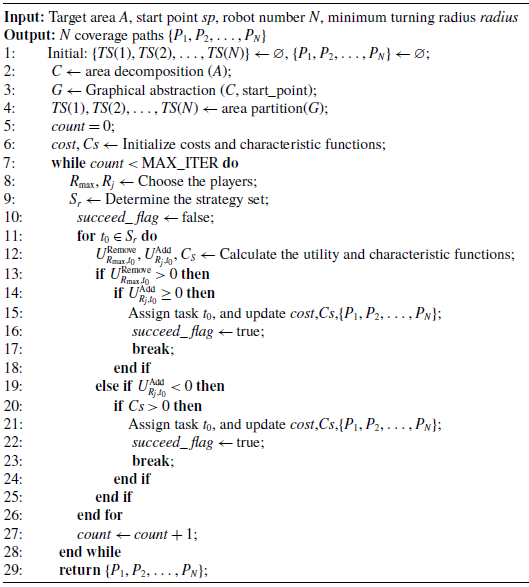
An algorithm for generating coverage paths for robots. The algorithm takes as input a target area A, a start point sp, the number of robots N, and the minimum turning radius of the robots. It outputs N coverage paths. The algorithm begins by initializing the tasks for each robot and then decomposes the area. It creates a graphical abstraction of the area and partitions it. The algorithm then initializes costs and characteristic functions. It iteratively chooses players, determines strategies, and assigns tasks to robots based on utility and characteristic functions. The process continues until a maximum number of iterations is reached or all tasks are successfully assigned.
4.4. Algorithmic pseudo-code
Algorithm1 shows the pseudo-code of GDM. GDM receives the target area
 $ A$
, the number of robots
 $ N$
, the starting point
 $ sp$
, the minimum turning radius
 $ radius$
, and initializes empty task and path sets (Line
 $ 1$
). Next, the Boustrophedon decomposition method is used to decompose the target area
 $ A$
into multiple rectangular cells (Line
 $2$
), which are then converted into a graph structure
 $ G$
(Line
 $3$
). Subsequently, the initial task set is obtained through area partition (Line
 $4$
). In the game negotiation phase, the algorithm initializes the iteration counter, cost function, and characteristic function (Lines
 $5-6$
). During each iteration, the robot with the maximum coverage time
 $ R_{\max }$
and the optional neighboring robot with the minimum coverage time
 $ R_{j}$
are selected as players (Line
 $8$
), and the strategy set
 $ C_s$
is determined (Line
 $9$
). For each task
 $ t_0$
in
 $ C_s$
, the values of the utility and characteristic functions are calculated (line
 $ 12$
), and the reallocation of the task is accepted or rejected based on the optimization objectives of the utility and characteristic functions (Lines
 $13-26$
). If accepted, the path set and the characteristic function are updated (Lines
 $15, 21$
). Finally, the algorithm returns the coverage path set for all robots
 $ \{P_1, P_2, \ldots , P_N\}$
(Line
 $ 29$
).
Computational complexity:
Assuming the area decomposition yields
 $M$
cells, the computational complexity of the area decomposition component is
 $O(M)$
, so is the area partition component. In the task fine-tuning component, the maximum outer iterations are
 $MAX\_ITER$
, while the inner loop operates in constant time. However, computing the utility and characteristic functions contains the process of solving the Dubins path, which makes a complexity of
 $O(M^3)$
. Consequently, the overall complexity of the algorithm is
 $O(MAX\_ITER\times M^3)$
.
5. Experiments
All experiments were conducted on a PC with an AMD Ryzen 7 7840H CPU and 32 GB RAM. The robot speed is set to
 $1.0$
m/s, the minimum turning radius is set to
 $0.5$
m, and the width of the task sensor
 $r_1$
is set to
 $1$
m. Three sets of experiments are performed to verify the performance of GDM: (1) comparative experiments in small-scale scenarios, (2) comparative experiments in medium and large-scale scenarios, and (3) feasibility experiment on a high-fidelity UAV platform.
5.1. Comparative experiments in small scale scenarios
Setup: This subsection tests the performance of the GDM algorithm in six scenarios on small scales. The size of all scenarios is
 $10 \times 10 \times 10$
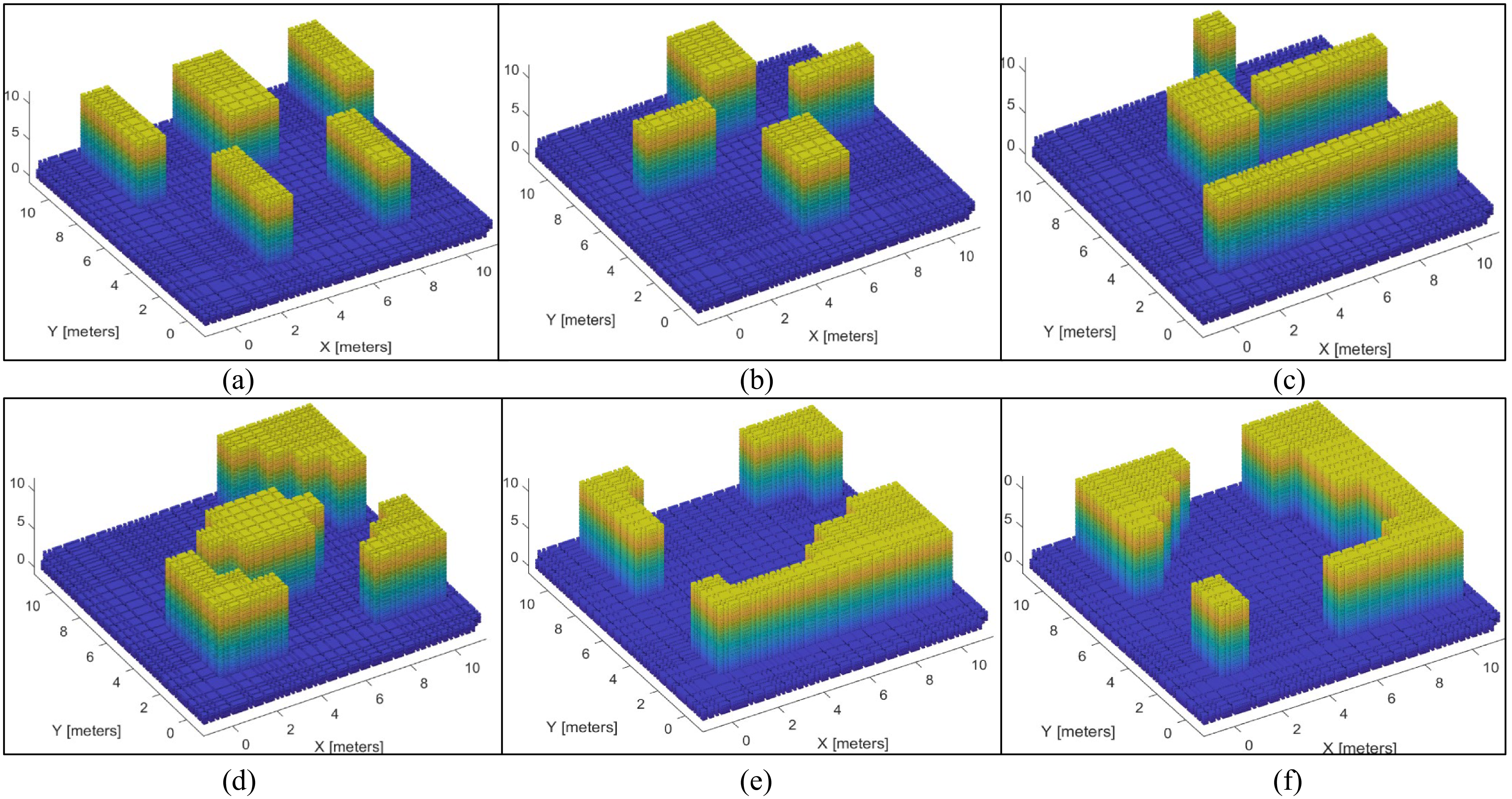
meters. Figure 8 shows all the scenes. The last two scenes are convex, and the others are non-convex. We evaluated the GDM algorithm using two and three robots.
We compare the GDM algorithm with the CDM [Reference Li, Shi, Jin, Yang, Zhou, Lian and Liu20], MILPFLOW [Reference Zhou, Wang, Ding, Hu and Shang24], EDM [Reference Li, Shi, Jin, Yang, Zhou, Lian and Liu20], and OM [Reference Choton and Prabhakar3] algorithms. The exact EDM and MILPFLOW algorithms were executed using Gurobi [54], with a maximum optimization time of 1,200 s. Furthermore, the LKH solver [Reference Helsgaun53] is utilized to compute the paths for GDM, CDM, and MILPFLOW. Since the OM algorithm is only applicable to convex scenarios, we first compared the GDM with other algorithms (excluding OM) in non-convex scenarios, then tested all algorithms in convex scenarios. Three metrics are used for performance evaluation as follows: (1) coverage time, (2) time equalization, and (3) computation time.
Cloud map of small scale scenarios. (a)–(d): Non-convex scenarios. (e)–(f): Convex scenarios.

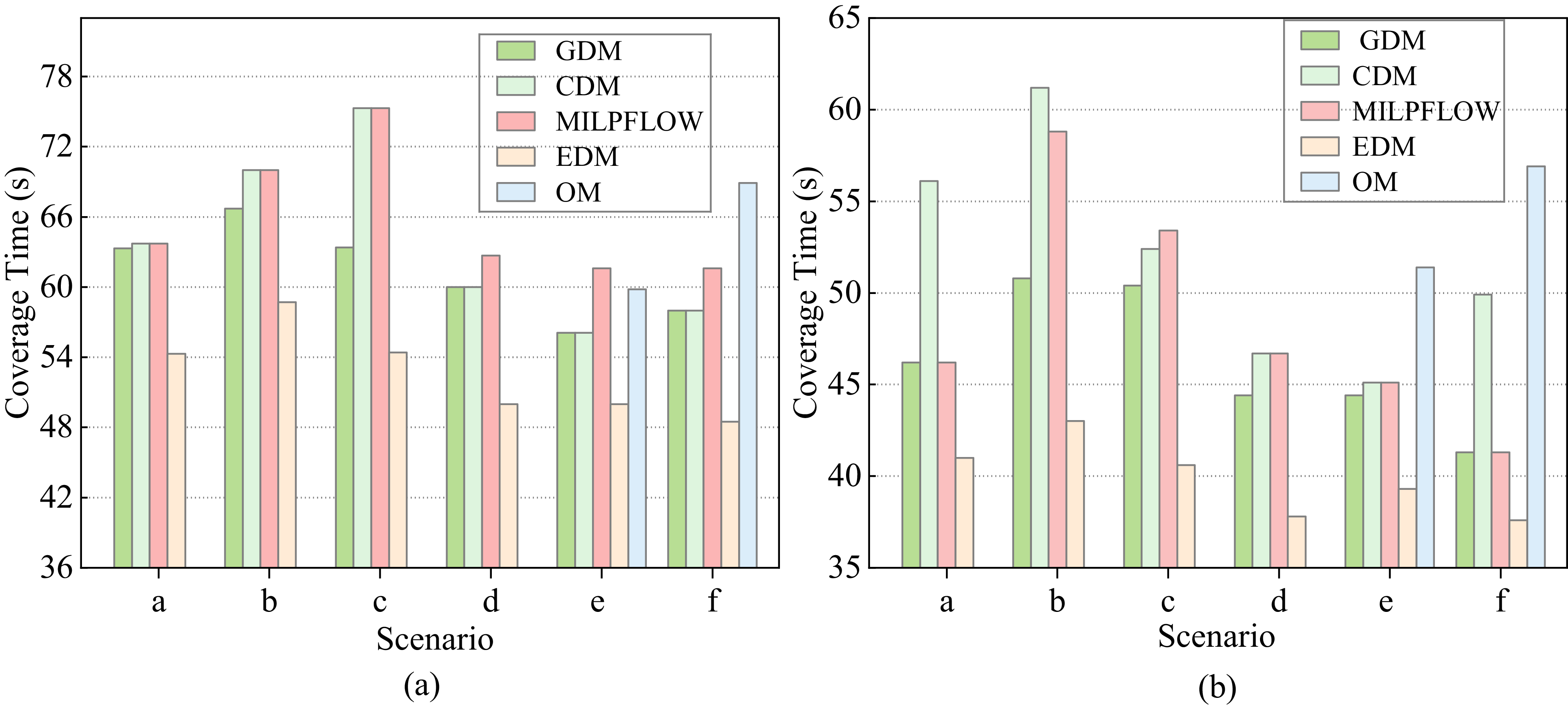
Comparison of coverage times for small-scale scenarios. (a) 2 robots. (b) 3 robots.

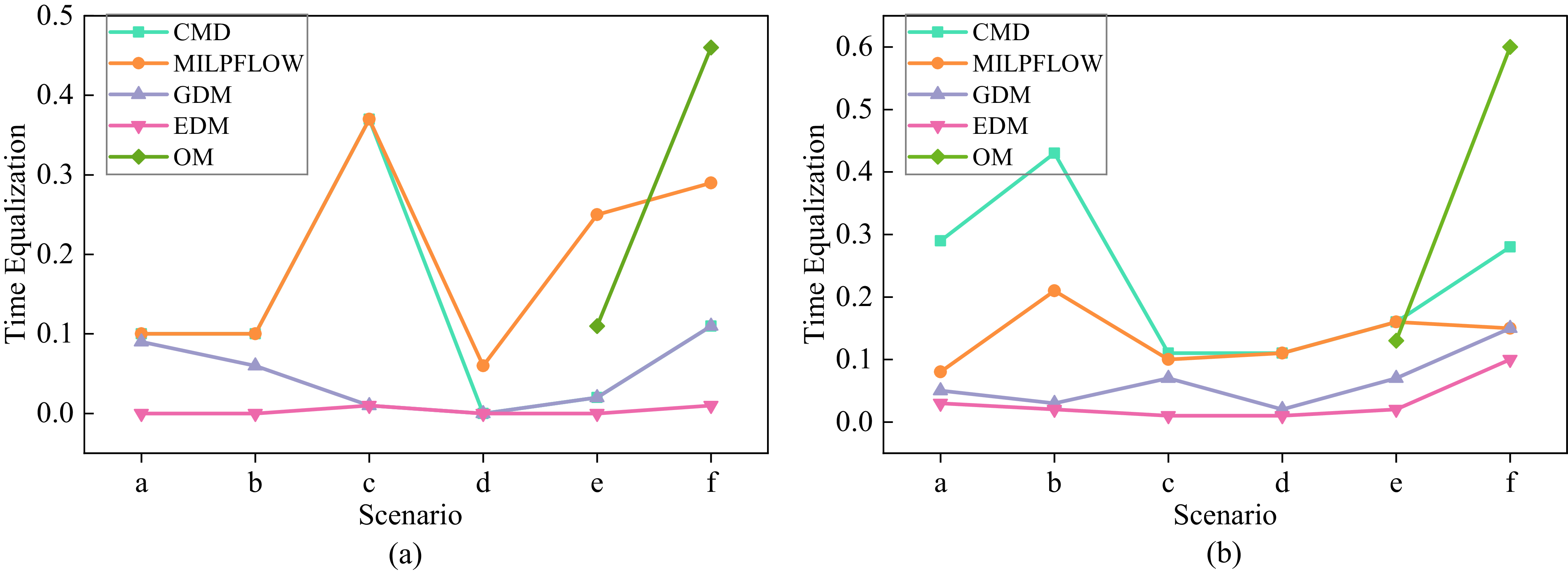
Comparison of time equalization for small-scale scenarios. (a) 2 robots. (b) 3 robots.

Results: Figure 9 shows the comparison results of coverage time in scenarios with different robots. The horizontal and vertical axes of Figure 9 represent different scenes and coverage times, respectively. Each sub-figure represents the comparison results with different numbers of robots. Apart from the exact algorithm EDM, it is observed that in all scenarios, the proposed GDM provides the shortest coverage time compared with other algorithms. When excluding exact algorithms, the coverage time of the GDM algorithm is reduced by approximately
 $7.8\%$
on average compared to other algorithms.
Figure 10 shows the comparison results of time equalization in scenarios with different robots. The horizontal and vertical axes represent different scenes and time equalization, respectively. Time equalization is measured using the coefficient of variation, which quantifies the dispersion of coverage times across all robots. A lower value indicates less disparity and a more balanced distribution. The experimental results reveal that, apart from the exact algorithm EDM, the proposed GDM can provide the best time equalization in all scenarios. Without considering the exact algorithm, the coverage time equalization of the GDM algorithm has been optimized by approximately
 $64.6\%$
compared to the average of other algorithms.
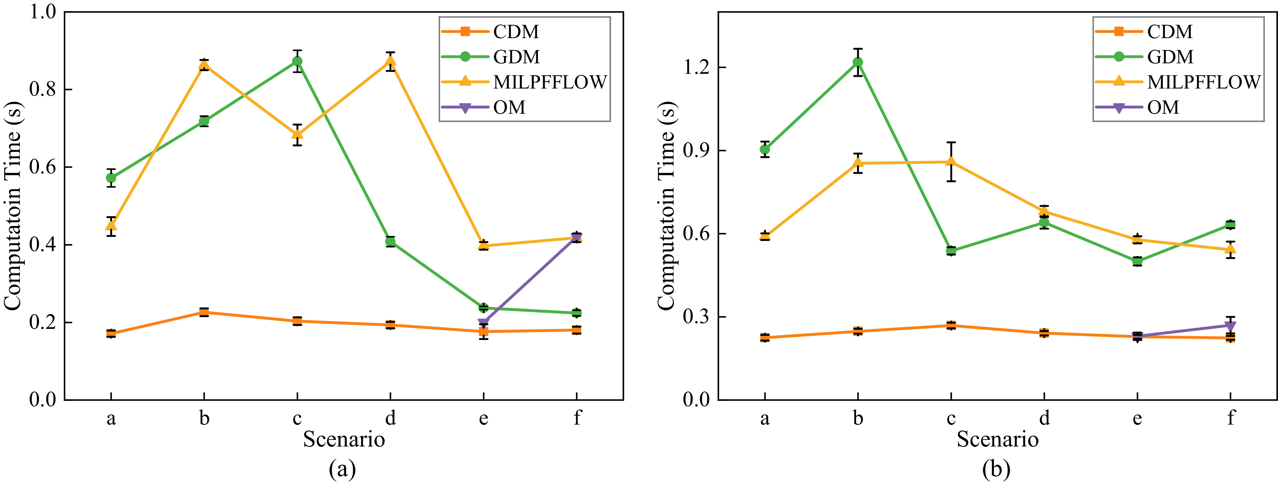
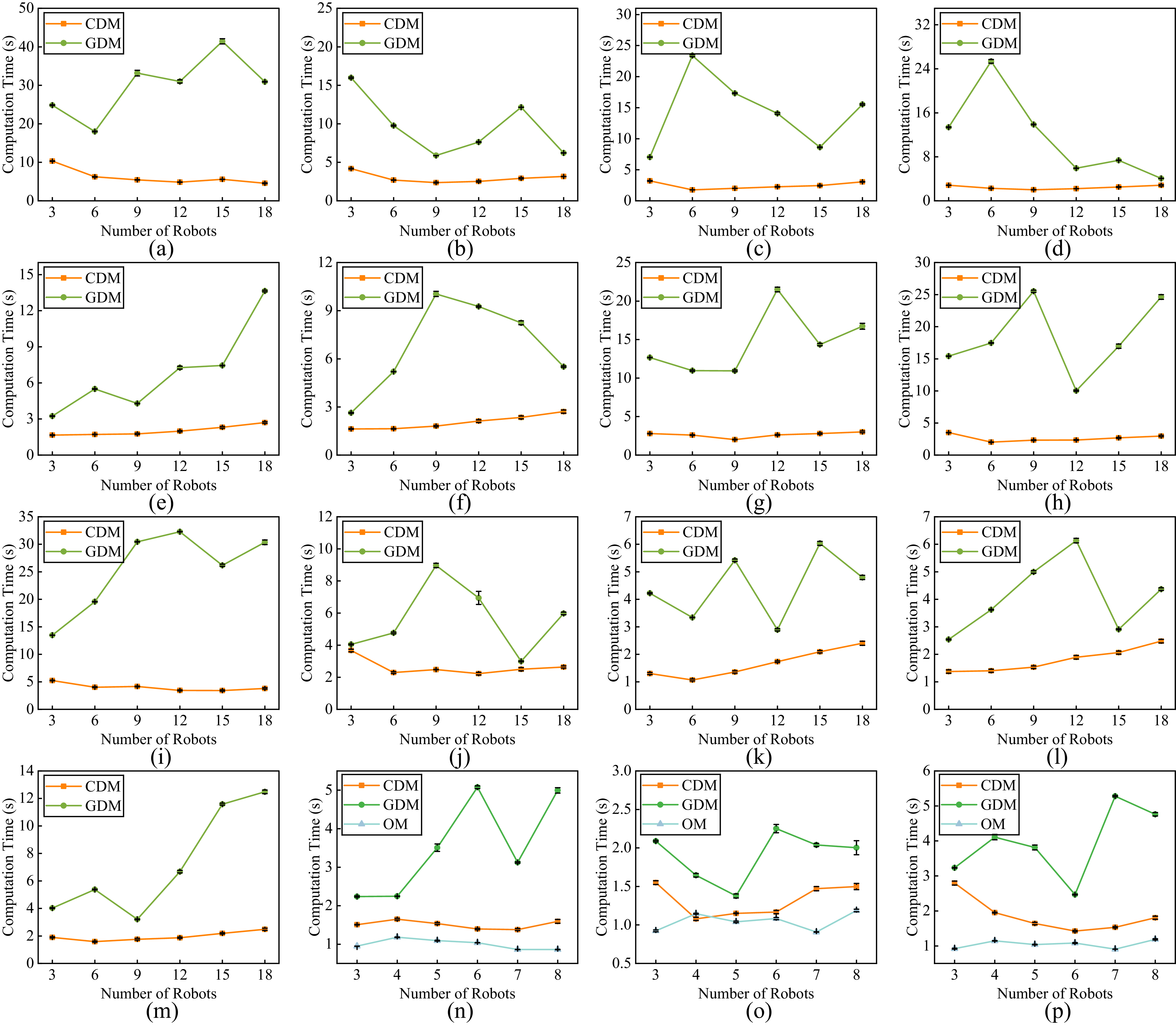
Figure 11 shows the comparison results of computation time in scenarios with different robots. The horizontal and vertical axes of Figure 11 represent different scenes and computation times, respectively. Since the computational time of the EDM algorithm reaches the predefined time limit (1,200 s) in the majority of scenarios, it has been excluded from the comparison in the figure. Although the computation time of the GDM algorithm increases slightly, which is attributed to the improvements made to the CDM algorithm, it achieves significantly better solution quality compared to other algorithms. It is worth emphasizing that even in the worst-case scenario, the solution time of GDM does not exceed 1.5 s.
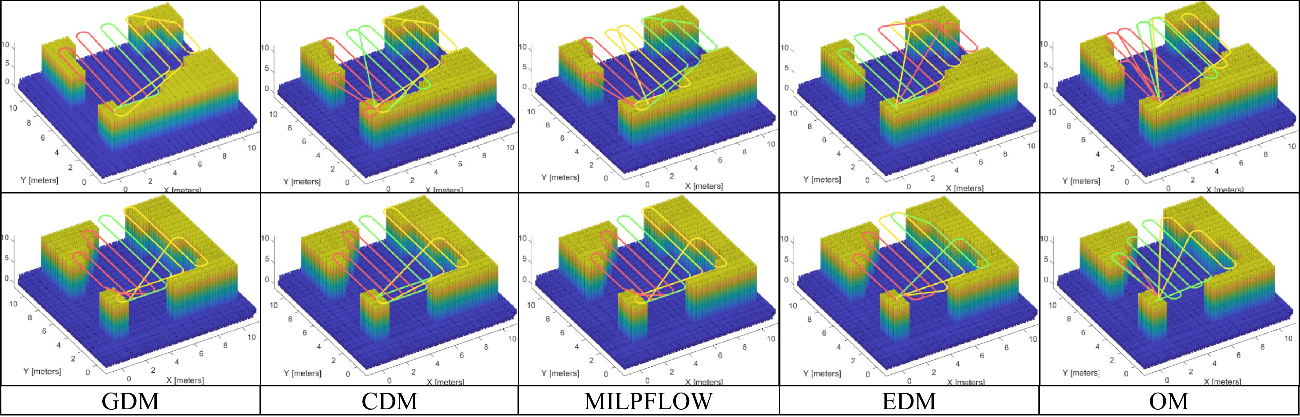
Figure 12 presents the coverage paths generated by different algorithms in small-scale environments. It can be observed that all methods generate smooth trajectories satisfying the Dubins curvature constraints. However, clear differences arise in terms of workload distribution and efficiency. Crucially, balanced area partitioning does not inherently equate to balanced path costs. While MILPFLOW and CDM focus on achieving spatially balanced sub-regions, they may overlook the impact of transition costs between cells, leading to less efficient results than GDM. In contrast, GDM directly balances the actual path costs through its game-theoretic mechanism, resulting in more equitable workloads and shorter completion times. Although EDM achieves theoretical optimum by directly minimizing path cost, its prohibitive computational overhead limits its practicality. Conversely, OM ignores workload balancing entirely, resulting in the most imbalanced paths and the longest coverage time. These observations are consistent with the quantitative results in Figure 9, demonstrating that GDM effectively bridges the gap between spatial balancing and path optimization.
Comparison of computation time for small-scale scenarios, with each scenario independently run 10 times. (a) 2 robots. (b) 3 robots.

Figure 11. Long description
Two line graphs compare computation times for small-scale scenarios involving 2 and 3 robots across different scenarios. Panel A: The line graph shows computation times for scenarios involving 2 robots. The x-axis is labeled Scenario with categories a to f, and the y-axis is labeled Computation Time (s) ranging from 0.0 to 1.0. Four lines represent different methods: CDM, GDM, MILPFFLOW, and OM. Panel B: The line graph shows computation times for scenarios involving 3 robots. The x-axis is labeled Scenario with categories a to f, and the y-axis is labeled Computation Time (s) ranging from 0.0 to 1.2. Four lines represent different methods: CDM, GDM, MILPFFLOW, and OM. Each scenario is independently run 10 times.
Path planning visualization for three robots across two different scenarios. Trajectories in different colors represent the paths of different UAVs. Each column (from left to right) corresponds to the GDM, CDM, MILPFLOW, EDM, and OM algorithms, respectively.

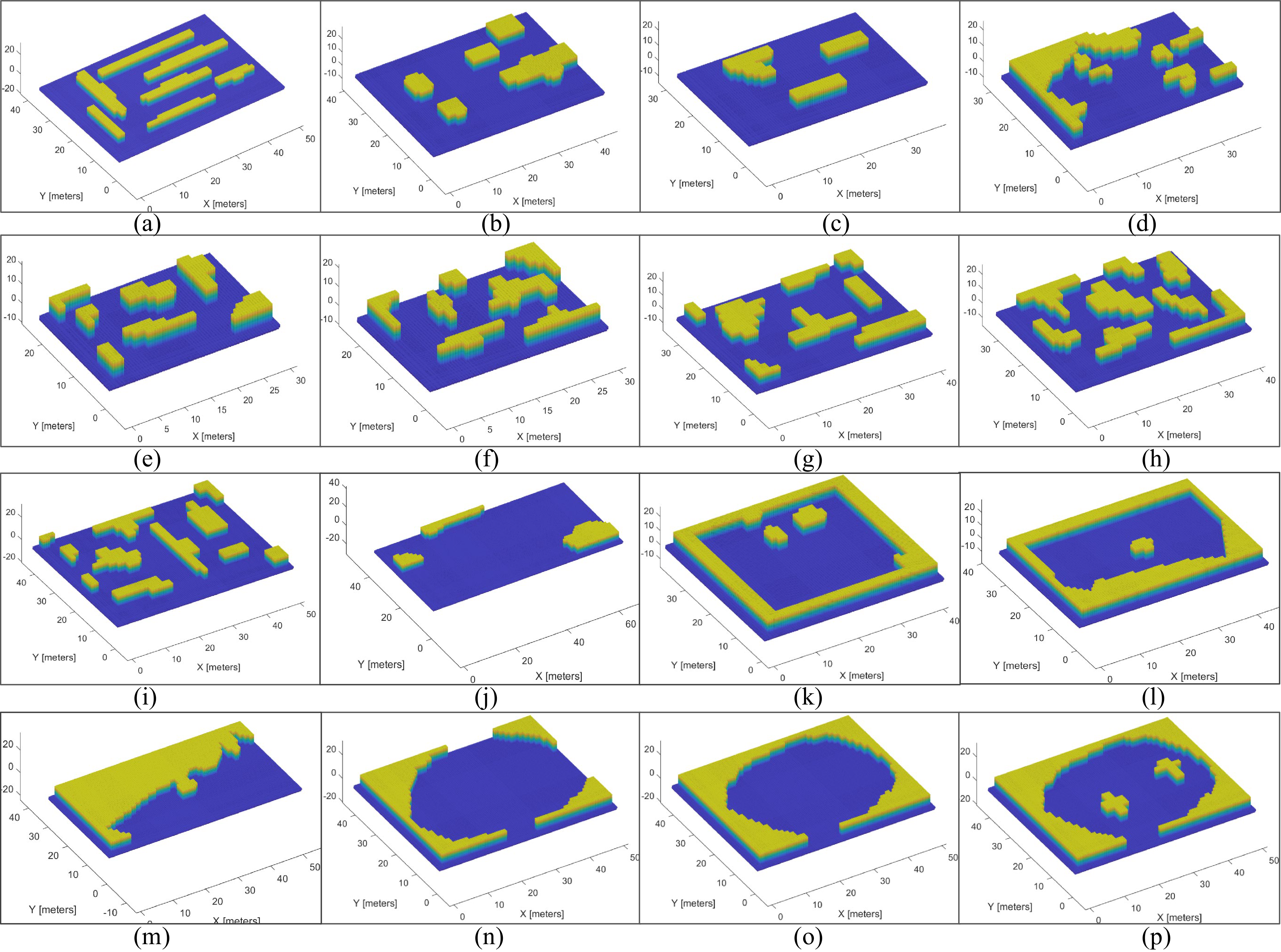
Test scenarios with medium and large scales. (a)–(m): Non-convex scenarios. (n)–(p): Convex scenarios.

Figure 13. Long description
Panel A: A 3D surface plot shows a non-convex scenario with yellow regions representing areas covered by robots and blue regions representing uncovered areas. The X and Y axes are labeled in meters, ranging from 0 to 50 meters. Panel B: Another 3D surface plot of a non-convex scenario with similar color coding and axis labels. Panel C: A 3D surface plot of a non-convex scenario with a different arrangement of covered and uncovered areas. Panel D: A 3D surface plot of a non-convex scenario with a more complex pattern of coverage. Panel E: A 3D surface plot of a non-convex scenario with varied coverage areas. Panel F: A 3D surface plot of a non-convex scenario with a different distribution of covered regions. Panel G: A 3D surface plot of a non-convex scenario with a distinct pattern of coverage. Panel H: A 3D surface plot of a non-convex scenario with a more intricate arrangement of covered areas. Panel I: A 3D surface plot of a non-convex scenario with a different layout of coverage. Panel J: A 3D surface plot of a convex scenario with a simpler pattern of coverage. Panel K: A 3D surface plot of a convex scenario with a different arrangement of covered regions. Panel L: A 3D surface plot of a convex scenario with a more uniform coverage pattern. Panel M: A 3D surface plot of a non-convex scenario with a varied distribution of covered areas. Panel N: A 3D surface plot of a convex scenario with a distinct pattern of coverage. Panel O: A 3D surface plot of a convex scenario with a different layout of covered regions. Panel P: A 3D surface plot of a convex scenario with a more complex arrangement of coverage.
5.2. Comparative experiments in medium and large scale scenarios
Setup: This subsection tests the performance of the GDM algorithm in 16 scenarios with medium and large scale. The dimensions of these scenarios are as follows: (a)
 $34$
m
 $\times 50$
m
 $\times 10$
m; (b)
 $34\,\text{m} \times 45\,\text{m} \times 10\,\text{m}$
; (c)
 $25\,\text{m} \times 38\,\text{m} \times 10\,\text{m}$
; (d)
 $25\,\text{m} \times 38\,\text{m} \times 10\,\text{m}$
; (e)
 $20\,\text{m} \times 30\,\text{m} \times 10\,\text{m}$
; (f)
 $20\,\text{m} \times 30\,\text{m} \times 10\,\text{m}$
; (g)
 $30\,\text{m} \times 40\,\text{m} \times 10\,\text{m}$
; (h)
 $30\,\text{m} \times 40\,\text{m} \times 10\,\text{m}$
; (i)
 $40\,\text{m} \times 50\,\text{m} \times 10\,\text{m}$
; (j)
 $36\,\text{m} \times 71\,\text{m} \times 10 \,\text{m}$
; (k)
 $37\,\text{m} \times 40\,\text{m} \times 10 \,\text{m}$
; (l)
 $32\,\text{m} \times 46\,\text{m} \times 10 \,\text{m}$
; (m)
 $29\,\text{m} \times 57\,\text{m} \times 10 \,\text{m}$
; (n)–(p)
 $40\,\text{m} \times 50\,\text{m} \times 10 \,\text{m}$
. All 16 scenarios are illustrated in Figure 13. Among them, scenarios (a)–(i) and (n)–(p) are generated simulated data, while scenarios (j)–(m) are derived from real farmland and provided by NEXAT GmbH [55]. The last three scenarios ((n)–(p)) are convex, and all others are non-convex. To verify the scalability of the GDM algorithm, we conducted experiments in twelve scenarios with varying numbers of robots. Specifically, for non-convex scenarios, the number of robots is set to 3, 6, 9, 12, 15, and 18; for convex scenarios, it is set to 3, 4, 5, 6, 7, and 8.
Due to the size of scenarios, MILPFLOW and EDM cannot provide the optimal solution within the limited time (1,200 s). Thus, we only compared the GDM algorithm with CDM and OM. Since OM algorithm is only applicable to convex scenarios, we first test GDM and CDM in non-convex scenarios(i.e., (a)–(m),) and then compare GDM, CDM, and OM in convex scenarios (i.e.,(n)–(p)). Three metrics are used for the performance evaluation, which are as follows: (1) coverage time, (2) time equalization, and (3) computation time.
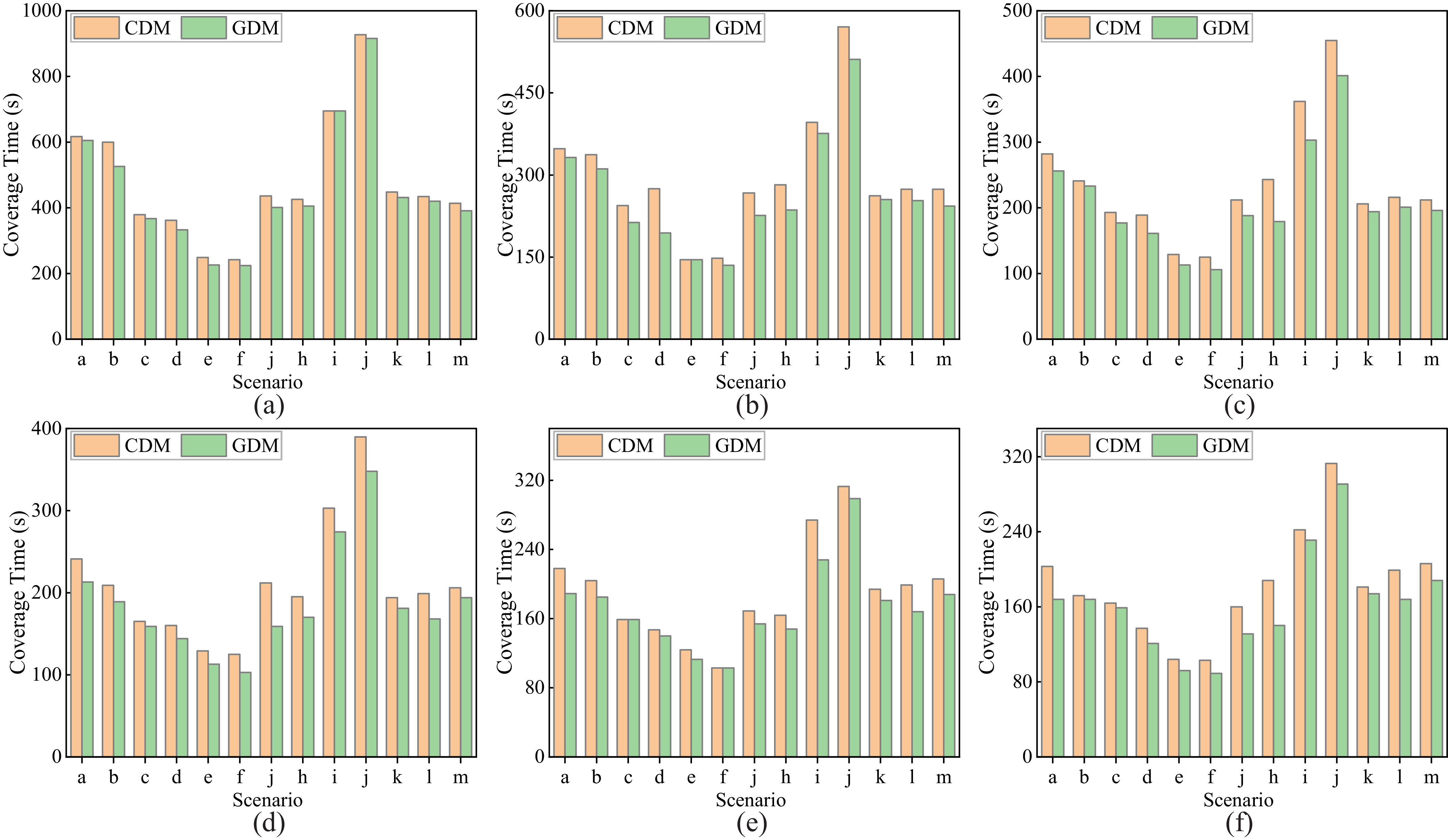
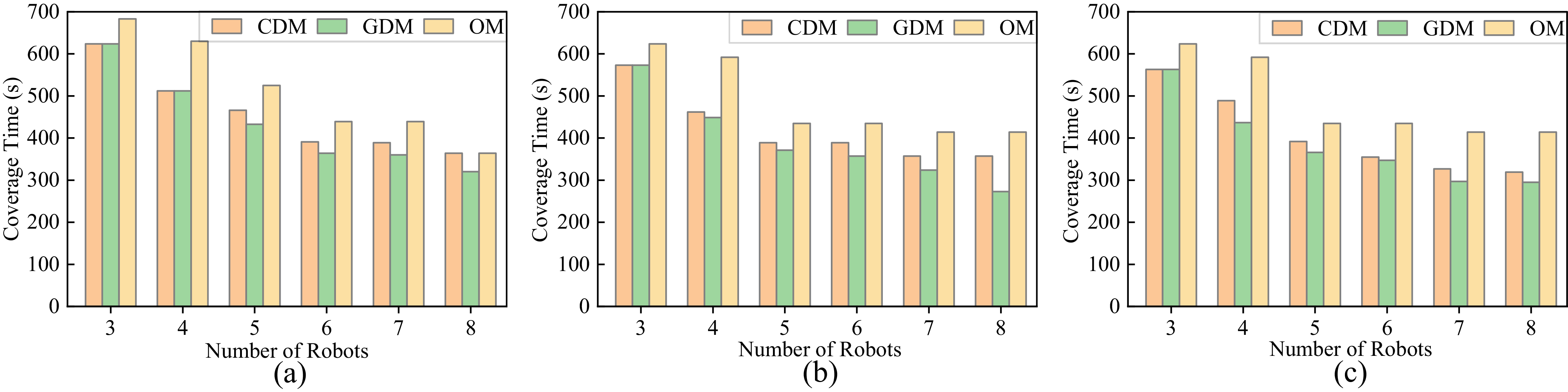
Results: Figures 15 and 16 show the comparison results of coverage time in scenarios with different robots. Each sub-figure represents the comparison results with different numbers of robots. It is observed that GDM provides the minimum coverage time than CDM and OM algorithms in all scenarios. Compared with other algorithms, the coverage time of the GDM algorithm has been reduced by approximately
 $10.8\%$
.
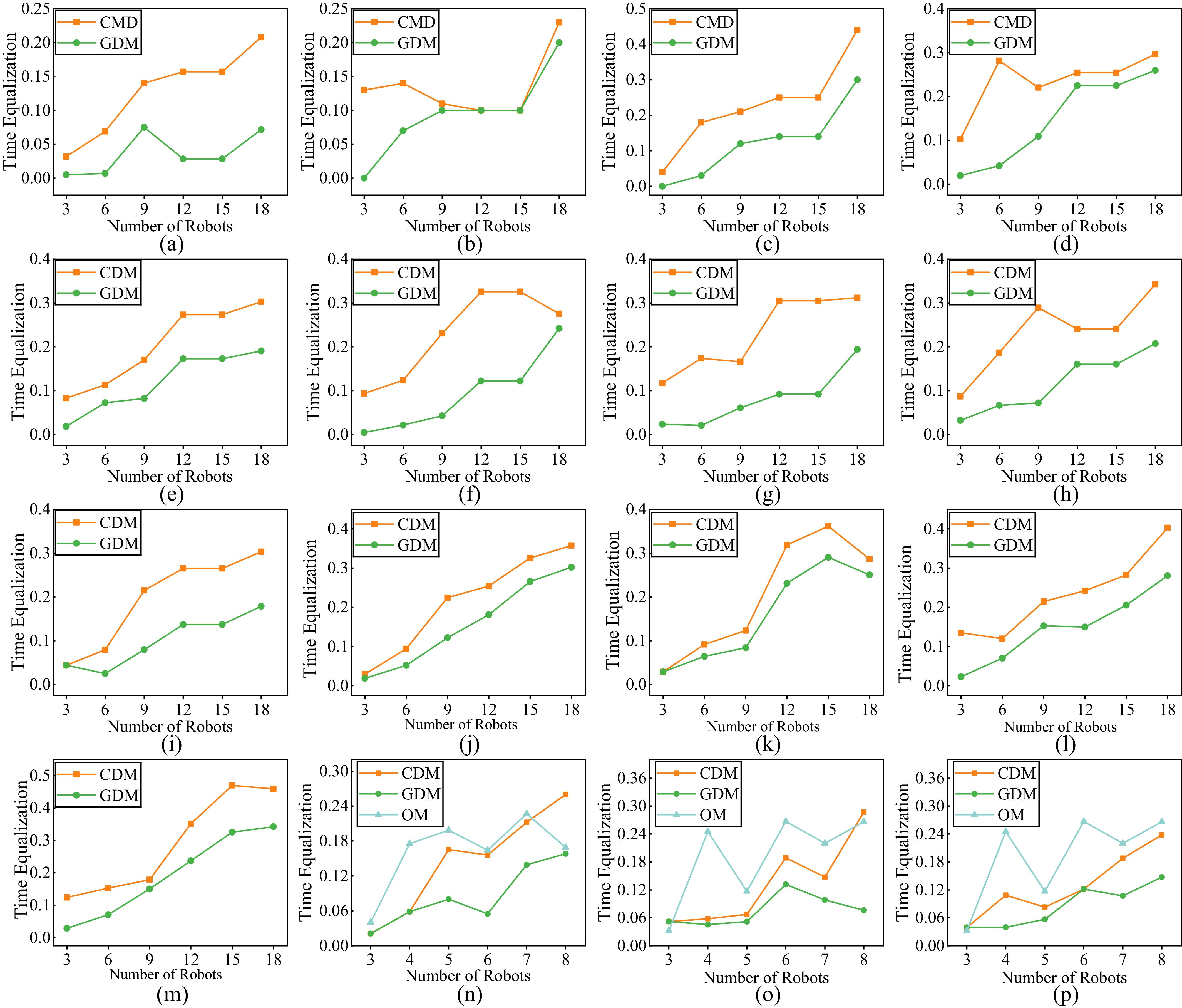
Figure 17 shows the results of the comparison of time equalization in scenarios with different robots. It is difficult for all algorithms to provide balanced coverage times for robots as the number of robots increases. However, GDM can provide the maximum time equalization in all experiments. Specifically, the time equalization of the GDM algorithm has been improved by
 $45.1\%$
compared to the average of other algorithms.
Comparison of coverage paths in convex scenarios with different numbers of robots. The first to third columns represent the coverage paths generated by GDM, CDM, and OM, respectively. The first row illustrates the results for six robots, and the second row illustrates the results for seven robots.

Figure 14. Long description
Panel A: The first column shows the coverage paths generated by GDM for six robots. The 3D plot has X and Y axes labeled in meters, ranging from 0 to 40 meters. The plot displays a colorful, grid-like pattern representing the coverage paths. Panel B: The second column shows the coverage paths generated by CDM for six robots. The 3D plot has X and Y axes labeled in meters, ranging from 0 to 40 meters. The plot displays a colorful, grid-like pattern representing the coverage paths. Panel C: The third column shows the coverage paths generated by OM for six robots. The 3D plot has X and Y axes labeled in meters, ranging from 0 to 40 meters. The plot displays a colorful, grid-like pattern representing the coverage paths. Panel D: The first column shows the coverage paths generated by GDM for seven robots. The 3D plot has X and Y axes labeled in meters, ranging from 0 to 40 meters. The plot displays a colorful, grid-like pattern representing the coverage paths. Panel E: The second column shows the coverage paths generated by CDM for seven robots. The 3D plot has X and Y axes labeled in meters, ranging from 0 to 40 meters. The plot displays a colorful, grid-like pattern representing the coverage paths. Panel F: The third column shows the coverage paths generated by OM for seven robots. The 3D plot has X and Y axes labeled in meters, ranging from 0 to 40 meters. The plot displays a colorful, grid-like pattern representing the coverage paths.
Comparison of coverage time in non-convex scenarios. (a)–(f) present the results with 3, 6, 9, 12, 15, and 18 robots, respectively.

Figure 15. Long description
The image contains six bar graphs comparing coverage time across different scenarios for varying numbers of robots. Each graph represents a different number of robots, ranging from 3 to 18. The x-axis of each graph is labeled with scenarios a to m, and the y-axis is labeled with coverage time in seconds. The graphs compare two methods, CDM and GDM, represented by orange and green bars respectively. Panel A shows results for 3 robots, Panel B for 6 robots, Panel C for 9 robots, Panel D for 12 robots, Panel E for 15 robots, and Panel F for 18 robots. Each panel displays variations in coverage time across different scenarios, with some scenarios showing significantly higher coverage times than others. The trends indicate that as the number of robots increases, the coverage time generally decreases, but the specific patterns vary across scenarios.
Comparison of coverage times in convex scenarios. (a)–(c) present the scenarios (n–(p), respectively.

Comparison of time equalization.

Figure 17. Long description
The image contains multiple line graphs comparing time equalization across different numbers of robots using various methods. Each graph plots time equalization on the vertical axis against the number of robots on the horizontal axis. The graphs are labeled from (a) to (p). Each graph includes two or three lines representing different methods: CMD, GDM, and OM. Panel A: A line graph showing time equalization for CMD and GDM methods. The horizontal axis represents the number of robots ranging from 3 to 18, and the vertical axis represents time equalization ranging from 0 to 0.25. Panel B: A line graph similar to Panel A but with a different dataset. Panel C: A line graph with time equalization ranging from 0 to 0.5. Panel D: A line graph with time equalization ranging from 0 to 0.4. Panel E: A line graph with time equalization ranging from 0 to 0.4. Panel F: A line graph with time equalization ranging from 0 to 0.4. Panel G: A line graph with time equalization ranging from 0 to 0.4. Panel H: A line graph with time equalization ranging from 0 to 0.4. Panel I: A line graph with time equalization ranging from 0 to 0.4. Panel J: A line graph with time equalization ranging from 0 to 0.4. Panel K: A line graph with time equalization ranging from 0 to 0.4. Panel L: A line graph with time equalization ranging from 0 to 0.4. Panel M: A line graph with time equalization ranging from 0 to 0.5. Panel N: A line graph with time equalization ranging from 0 to 0.3. Panel O: A line graph with time equalization ranging from 0 to 0.36. Panel P: A line graph with time equalization ranging from 0 to 0.36. Each panel shows the trends and patterns of time equalization as the number of robots increases, with CMD generally showing higher time equalization compared to GDM and OM methods.
Comparison of computation time. For each scenario, the algorithm is independently run 10 times.

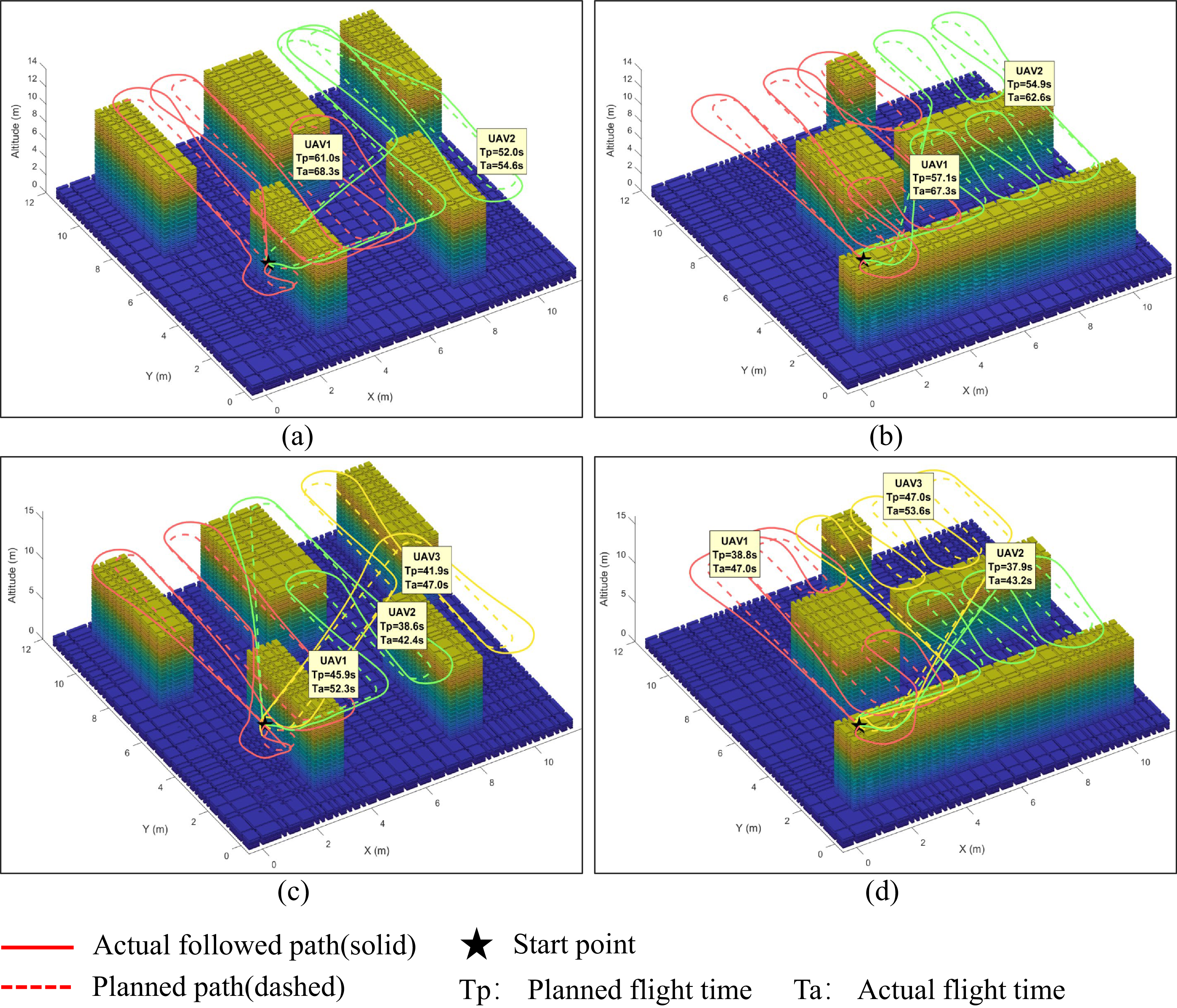
Feasibility experiments in small-scale scenarios. The dashed lines represent the planned paths, and the solid lines show the actual trajectories of the UAVs.
 $T_p$
and
 $T_a$
denote the planned time and the actual flight time, respectively. (a) and (b): 2 robots; (c) and (d): 3 robots.

Figure 19. Long description
Panel A: A 3D plot depicts the planned and actual paths of two UAVs navigating through a complex environment. The x-axis represents the X coordinate in meters, the y-axis represents the Y coordinate in meters, and the z-axis represents the altitude in meters. The planned paths are shown as dashed lines, while the actual followed paths are shown as solid lines. The plot includes labels for UAV1 and UAV2, with their respective planned and actual flight times indicated. Panel B: Another 3D plot shows the planned and actual paths of two UAVs in a different configuration. The axes and line styles are consistent with Panel A. The plot includes labels for UAV1 and UAV2, with their respective planned and actual flight times indicated. Panel C: A 3D plot depicts the planned and actual paths of three UAVs navigating through the environment. The axes and line styles are consistent with the previous panels. The plot includes labels for UAV1, UAV2, and UAV3, with their respective planned and actual flight times indicated. Panel D: Another 3D plot shows the planned and actual paths of three UAVs in a different configuration. The axes and line styles are consistent with the previous panels. The plot includes labels for UAV1, UAV2, and UAV3, with their respective planned and actual flight times indicated.
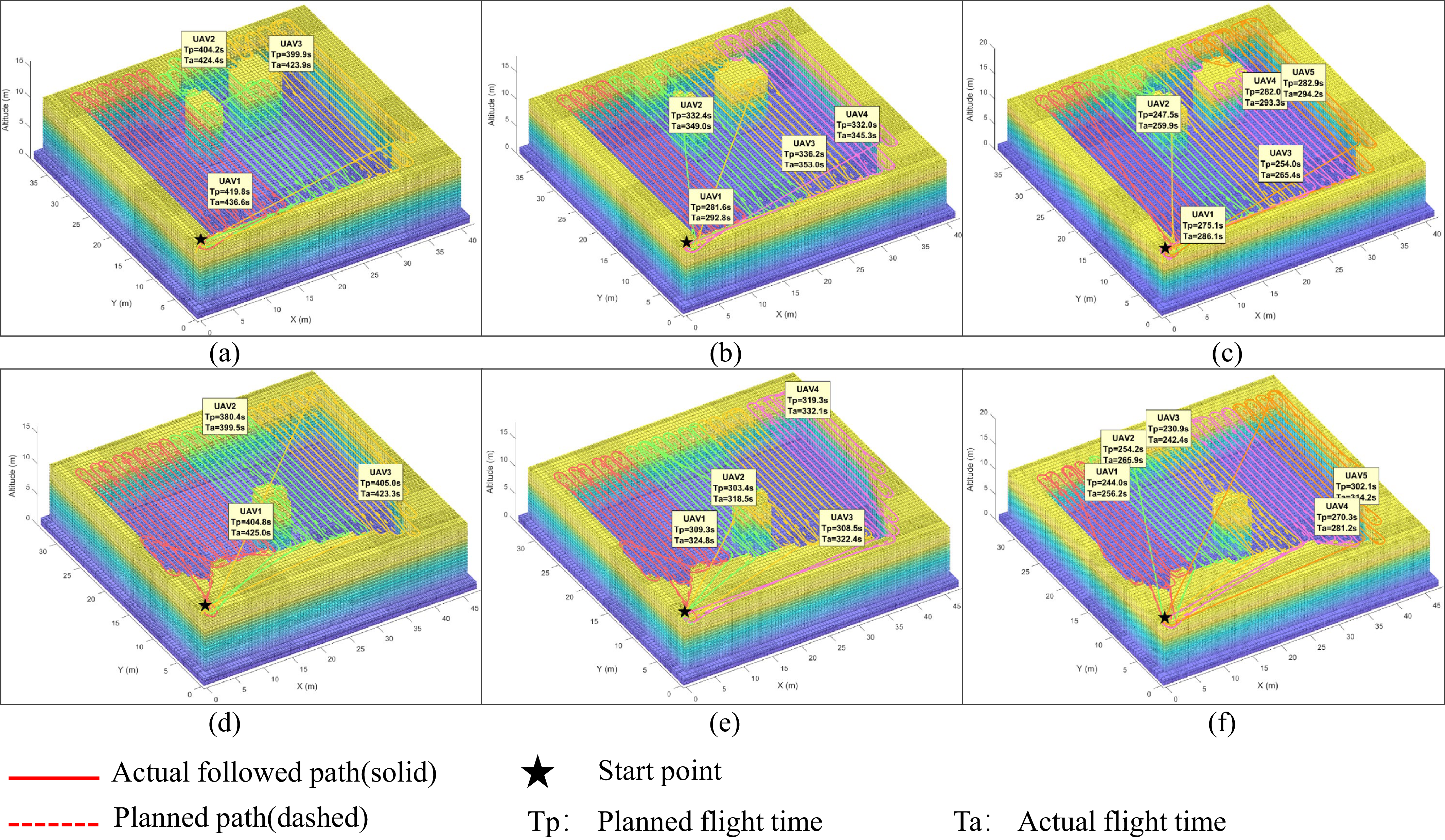
Feasibility experiments in large-scale scenarios. The dashed lines represent the planned paths, and the solid lines show the actual trajectories of the UAVs.
 $T_p$
and
 $T_a$
denote the planned time and the actual flight time, respectively. (a) and (d): 3 robots; (b) and (e): 4 robots; (c) and (f): 5 robots.

Figure 18 shows the comparison of the computation time in each scenario. It is seen that OM provides the minimum computation time in convex scenarios (n)-(p). This is because the OM algorithm eliminates the planning process. Instead, it directly moves back and forth within the partitioned sub-areas to accomplish coverage tasks, which makes the worst coverage time among all methods. Meanwhile, GDM produces a higher computation time than CDM and OM. This is because GDM needs to play multiple rounds of games based on CDM to improve the quality of the solution. In other words, GDM achieves higher calculation accuracy at the cost of increasing calculation time. However, even in the worst-case scenario, the GDM algorithm completes the solution within 40 s, and in several tested convex areas, the solving time is less than 5 s. This is because we set fewer obstacles in the non-convex scenarios than in the convex ones; thus, the environmental complexity in non-convex scenarios is lower, making it easier to plan paths. This is consistent with farmland scenes, which rarely contain numerous or complex obstacles. Compared to the exact algorithm, which requires thousands of seconds, GDM significantly reduces the solution time while maintaining solving accuracy.
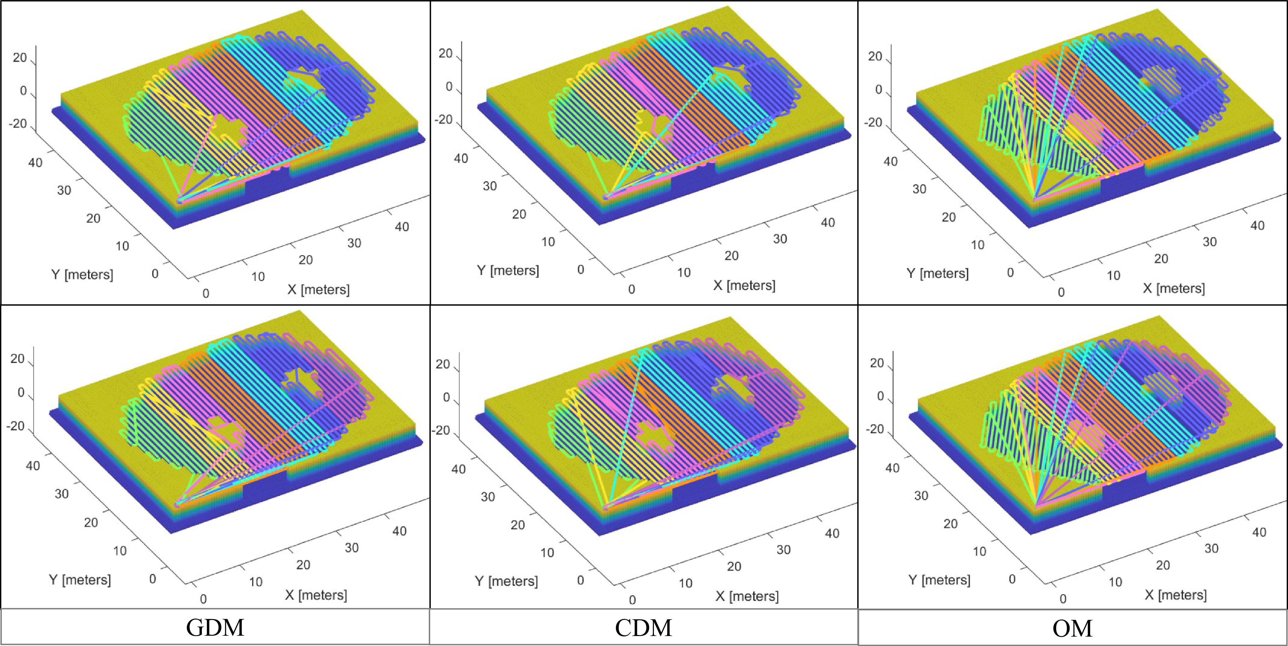
Figure 14 shows the coverage paths generated by different algorithms in large-scale multi-robot environments. It can be observed that GDM achieves a well-balanced workload distribution among robots, resulting in similar path lengths and execution times. In contrast, the baseline methods exhibit clear limitations. CDM only focuses on balanced area partitioning. However, a balanced geometric area does not equal a balanced coverage time, which still leads to workload mismatches. Meanwhile, OM completely ignores area balancing during partitioning. As a result, it suffers from severe workload imbalances among the robots. These observations are consistent with the quantitative results shown in Figures 16 and 17. Furthermore, as the number of robots increases, GDM maintains consistent partitioning quality, demonstrating strong scalability in large-scale settings.
5.3. Feasibility experiment
Setup: We validate the proposed GDM algorithm using a high-fidelity fixed-wing UAV model [Reference Romero56] in simulation. A waypoint-following controller is employed to track the generated coverage paths. The UAVs are constrained by a constant forward speed of
 $1$
m/s and a minimum turning radius of
 $0.5$
m. To comprehensively evaluate the performance, experiments are conducted in both small-scale and large-scale scenarios. In the small-scale setting, two environments of size
 $10 \times 10$
m are tested, each with
 $2$
and
 $3$
UAVs, respectively. In the large-scale setting, we consider two distinct environments derived from real-world farmland scenarios [55]: the first with a size of
 $37 \times 40$
m (Figure 20(a)–(c)) and the second with
 $32 \times 46$
m (Figure 20(d)–(f)), where
 $3$
,
 $4$
, and
 $5$
UAVs are deployed. All UAVs share a common start location and are assigned different flight altitudes to ensure collision avoidance. The generated coverage paths are directly used as reference trajectories for the UAV controller.
Results: The experimental results are illustrated in Figures 19 and 20. The dashed colored lines represent the planned coverage paths generated by GDM, while the solid colored lines denote the actual executed trajectories of the UAVs.
For each UAV, we report both the planned coverage time (
 $T_p$
) and the actual flight time (
 $T_a$
). The results show that all UAVs are able to accurately follow the planned paths under curvature constraints. Although minor deviations between
 $T_p$
and
 $T_a$
are observed due to dynamic and tracking effects, the differences remain small across all scenarios. These results demonstrate that the planned paths are not only geometrically feasible but also dynamically executable for Dubins robots, such as fixed-wing UAVs.
6. Conclusions
Aiming at the problem of CPP for multiple curvature-constrained robots in known agricultural environments, this study first proposes an exact mathematical model, which can solve the optimal path for robots. Then a heuristic MCPP method based on game theory, i.e., the GDM algorithm, is proposed. The GDM algorithm first employs area growing and tree partitioning strategies to obtain an approximate equilibrium area partitioning result and then takes a game-based strategy for task reallocation to plan a balanced, efficient, and kinematically smooth path for robots. Through comparative experiments across varying scenario scales, we evaluate the performance of the GDM algorithm and verify the feasibility on a high-fidelity UAV model. Our experimental results demonstrate that the proposed method achieves shorter coverage time, improves task load balancing significantly, and the planned path satisfies the robotic curvature constraints.
Data availability statement
The data that support the findings of this study are available from the corresponding author upon reasonable request.
Author contributions
Author Yahui Li: - conceived and designed the study, developed the methodology, and wrote the original draft; Lin Li : - contributed to the methodology and investigation, and provided supervision; Shihao Xiong : - and Mengbo Ma performed data curation and validation; Yishu Yan, Yangrui Meng and Haoxiang Jin: - participated in review and editing of the manuscript. Haoxiang Jin: - also acquired the funding. All authors reviewed and approved the final manuscript.
Financial support
This work was supported by the Key Project of Hunan Provincial Department of 471 Education (grant number 24A0671).
Competing interests
The authors declare no competing interests.
Ethical approval
Not applicable.


 Tp
 Ta
 Tp
 Ta


