1. Introduction
Active wall deformations with appropriate parameters have the ability to reduce the skin-friction drag of wall-bounded turbulent flows (Abdulbari et al. Reference Abdulbari, Yunus, Abdurahman and Charles2013; Zhang, Shan & Xie Reference Zhang, Shan and Xie2020; Ricco, Skote & Leschziner Reference Ricco, Skote and Leschziner2021). It is known that a travelling wave can reduce the drag when it propagates in the streamwise direction and its amplitude is in the wall-normal direction (Fukagata, Iwamoto & Hasegawa Reference Fukagata, Iwamoto and Hasegawa2024). Drag-reducing travelling waves can be realised through blowing and suction (Mamori, Iwamoto & Murata Reference Mamori, Iwamoto and Murata2014; Koganezawa et al. Reference Koganezawa, Mitsuishi, Shimura, Iwamoto, Mamori and Murata2019), wall deformations (Nakanishi, Mamori & Fukagata Reference Nakanishi, Mamori and Fukagata2012; Nabae, Kawai & Fukagata Reference Nabae, Kawai and Fukagata2020) and body forces (Mamori & Fukagata Reference Mamori and Fukagata2014). The travelling wave control focused on in this study is sinusoidal wall deformations in the wall-normal direction according to
 \begin{equation} y_{{wall}} = \eta \cos (\phi ), \end{equation}
where
 $\phi$
is the phase of wall motion defined as
 \begin{equation} \phi = \frac {2 \pi }{\lambda } (x - ct), \end{equation}
 $x$
is the streamwise location,
 $t$
is the time,
 $\eta$
is the amplitude,
 $\lambda$
is the wavelength and
 $c$
is the wave speed. Travelling wave control is known to stabilise the fully developed channel flow, leading to relaminarisation (Lee, Min & Kim Reference Lee, Min and Kim2008; Moarref & Jovanović Reference Moarref and Jovanović2010). The effective parameters of the travelling wave to bring about the relaminarisation phenomena are reported as amplitude in wall units of
 $3 \lt \eta ^+ \lt 10$
, wavelength in wall units of
 $200 \lt \lambda ^+ \lt 500$
and wave speed normalised by the centre velocity of the corresponding laminar flow of
 $c/U_{{c,\ lam}} \geq 1$
(Nakanishi et al. Reference Nakanishi, Mamori and Fukagata2012; Mamori et al. Reference Mamori, Iwamoto and Murata2014).
Recently, turbulent boundary-layer flow over a travelling wavy-wall deformation achieved drag reduction by 9.4 % in total (Yoshida et al. Reference Yoshida, Nimura, Mitsuishi, Murata and Iwamoto2025), which was evaluated using the streamwise integral of the von Kármán momentum integral. This reduction in total drag was attributed to reduced turbulent skin friction, likely overcoming the profile drag caused by the wavy wall. They generated the effective parameter sets of the travelling wave by using an oscillated rubber sheet, i.e. amplitude, wavelength and wave speed, proposed in fully developed turbulent pipes or channels (Nakanishi et al. Reference Nakanishi, Mamori and Fukagata2012; Mamori et al. Reference Mamori, Iwamoto and Murata2014; Koganezawa et al. Reference Koganezawa, Mitsuishi, Shimura, Iwamoto, Mamori and Murata2019). Turbulence statistics in the previous experiment (Yoshida et al. Reference Yoshida, Nimura, Mitsuishi, Murata and Iwamoto2025) were obtained at the streamwise location after 0.7 m of control, of which length is approximately equivalent to 12 times the wavelength of the travelling wave. In the downstream location, the random Reynolds shear stress (RSS) is reduced across the boundary layer, which indicates that modification of the flow in the near-wall region suppresses the turbulent motions in the outer region. However, the turbulence-suppression process in the streamwise direction is unclear because of the lack of measurement locations.
Among the previous studies on travelling wave control (Nakanishi et al. Reference Nakanishi, Mamori and Fukagata2012; Mamori et al. Reference Mamori, Iwamoto and Murata2014; Koganezawa et al. Reference Koganezawa, Mitsuishi, Shimura, Iwamoto, Mamori and Murata2019), the flow characteristics are often analysed using a three-component decomposition (Hussain & Reynolds Reference Hussain and Reynolds1970) for instantaneous velocities as follows:
 \begin{eqnarray} \boldsymbol{u} &=& \bar {\boldsymbol{u}} + \tilde {\boldsymbol{u}} + \boldsymbol{u}^{\prime\prime}, \end{eqnarray}
where
 $\bar {\boldsymbol{u}}$
is the time-averaged velocity,
 $\tilde {\boldsymbol{u}}$
is the periodic velocity fluctuation and
 $\boldsymbol{u}^{\prime\prime}$
is the random velocity fluctuation. This decomposition reveals that travelling wave control directly generates a periodic flow motion accompanied by a wavy forcing from the wall and secondarily reduces a random fluctuation representing a typical turbulent motion in the wall turbulence. In previous studies on turbulent internal flows under streamwise-periodic conditions, a stable drag-reduction effect was observed after approximately 100–800 periods of control application (Nakanishi et al. Reference Nakanishi, Mamori and Fukagata2012; Mamori et al. Reference Mamori, Iwamoto and Murata2014; Koganezawa et al. Reference Koganezawa, Mitsuishi, Shimura, Iwamoto, Mamori and Murata2019). This delayed response suggests a sequence where the directly induced periodic flow gradually modifies the existing turbulent structures, leading to a reduction in random fluctuations and, ultimately, drag reduction.
The transient process of the random fluctuation suppression over the travelling wave has not been investigated in the temporal or streamwise-developing context. In turbulent boundary-layer flow, observation in the streamwise direction is equivalent to time evolution observation in streamwise-periodic turbulent internal flows (Kim & Hussain Reference Kim and Hussain1993; Skote Reference Skote2012). The modification process of turbulence after a sudden change of the wall configuration is thoroughly studied on smooth walls to rough walls (and vice versa) (Antonia & Luxton Reference Antonia and Luxton1971; Smits & Wood Reference Smits and Wood1985; Lee Reference Lee2015; Hanson & Ganapathisubramani Reference Hanson and Ganapathisubramani2016; Li et al. Reference Li, de Silva, Chung, Pullin, Marusic and Hutchins2022) from the viewpoint of an internal boundary layer (IBL). The IBL is an internal layer that reflects the effect of the wall change within the 99 % boundary-layer thickness. The thickness of the internal layer is referred to as the IBL thickness
 $\delta _{{i}}$
, whose streamwise development is often described by a power law:
 \begin{equation} \delta _{{i}} (x) = a x^b, \end{equation}
where
 $a$
is the coefficient and
 $b$
is the exponent. Meanwhile, studies on the transient process after the wall change for drag reduction by suppressing turbulent fluctuations through opposition controls (Fukagata & Kasagi Reference Fukagata and Kasagi2003; Ge, Tian & Yongqian Reference Ge, Tian and Yongqian2016) and spanwise wall oscillations (Quadrio & Ricco Reference Quadrio and Ricco2003; Xu & Huang Reference Xu and Huang2005; Stroh et al. Reference Stroh, Hasegawa, Schlatter and Frohnapfel2016) have been conducted.
In the present study, modification of turbulent boundary-layer flow by travelling wave control was measured using particle image velocimetry (PIV). Measurements are performed at multiple streamwise locations in a developing turbulent boundary-layer flow over the travelling wave generated on a rubber sheet following the methodology in a previous study (Yoshida et al. Reference Yoshida, Nimura, Mitsuishi, Murata and Iwamoto2025). The travelling wave parameters are within the range of occurrence of relaminarisation for fully developed turbulent pipes or channels (Nakanishi et al. Reference Nakanishi, Mamori and Fukagata2012; Mamori et al. Reference Mamori, Iwamoto and Murata2014; Koganezawa et al. Reference Koganezawa, Mitsuishi, Shimura, Iwamoto, Mamori and Murata2019). The objective of the present study is to reveal a process to alter the turbulent structure and to reduce the random fluctuations by periodic manipulation of travelling wave control in spatially developing boundary-layer flow.
2. Experimental set-up
The present study is performed in an open-return turbulent boundary-layer wind tunnel with zero pressure gradient. This wind tunnel was designed to achieve an effective travelling wave so that its non-dimensional properties fall within the effective range (described in § 2.1), i.e. a free-stream velocity
 $U_\infty = 2$
m s−1 and a friction velocity
 $u_\tau$
in the test section of approximately 0.1 m s−1 such that achievable travelling wave parameters meet the range to relaminarise turbulent internal flows (Nakanishi et al. Reference Nakanishi, Mamori and Fukagata2012; Mamori et al. Reference Mamori, Iwamoto and Murata2014; Koganezawa et al. Reference Koganezawa, Mitsuishi, Shimura, Iwamoto, Mamori and Murata2019). Using the present facilities, a 9.4 % reduction in drag due to the travelling wave is achieved in relation to previous literature (Yoshida et al. Reference Yoshida, Nimura, Mitsuishi, Murata and Iwamoto2025).
2.1. Travelling wavy wall
(upper left) Schematic of generation mechanism and visualisation procedure of travelling wavy wall (not to scale) and (lower right) snapshot of visualised travelling wave using a laser sheet.

The travelling wave is generated on the rubber sheet using a piezoelectric actuator (APA-1000L, Cedrat Technologies) glued to the upstream edge of the sheet. We chose a piezoelectric actuator because of its high repeatability of oscillation. The characteristics of the travelling wave are determined by the physical properties of the rubber sheet, the tension and the oscillating frequency of the piezoelectric actuator
 $f$
. This study used a polychloroprene rubber sheet (NEO-180, Irumagawa Rubber Co. Ltd), with a thickness of 0.3 mm, a tensile strength of
 $8.0\ \mathrm{MPa}$
and an elongation rate of
 $300\,\%$
. Yoshida et al. (Reference Yoshida, Nimura, Mitsuishi, Murata and Iwamoto2025) used the same rubber sheet to generate a travelling wave within the range of the relaminarisation reported in Nakanishi et al. (Reference Nakanishi, Mamori and Fukagata2012) and Mamori et al. (Reference Mamori, Iwamoto and Murata2014), with an appropriate tensioning force per surface area of
 $0.018\ \mathrm{kg\,m^{-2}}$
and
 $f=150$
Hz. Figure 1 shows a snapshot of the visualised travelling wave and a schematic illustration of how it is obtained. Here, crests of the travelling wave are illuminated in green by a laser sheet generated by a Nd:YAG laser irradiated at a shallow angle.
Quasi-instantaneous wall-normal deformation of the travelling wavy wall.

Figure 2 shows a profile of the wall deformation
 $y_{{wall}}^+$
, which can be considered a quasi-instantaneous waveform because of measurements using a high-speed two-dimensional laser profiler (LJ-V7300, KEYENCE Corp.) synchronised with the vibration source. Here, the wall deformation and the spanwise location are normalised in wall units at
 $x=0$
. The wave was adjusted in the same manner as in Yoshida et al. (Reference Yoshida, Nimura, Mitsuishi, Murata and Iwamoto2025), and the present waveform is considered an optimal case in terms of its spanwise uniformity. The resultant turbulent feature in the downstream region is similar when the wave properties are comparable with previously proposed ranges (Nakanishi et al. Reference Nakanishi, Mamori and Fukagata2012; Mamori et al. Reference Mamori, Iwamoto and Murata2014; Koganezawa et al. Reference Koganezawa, Mitsuishi, Shimura, Iwamoto, Mamori and Murata2019).
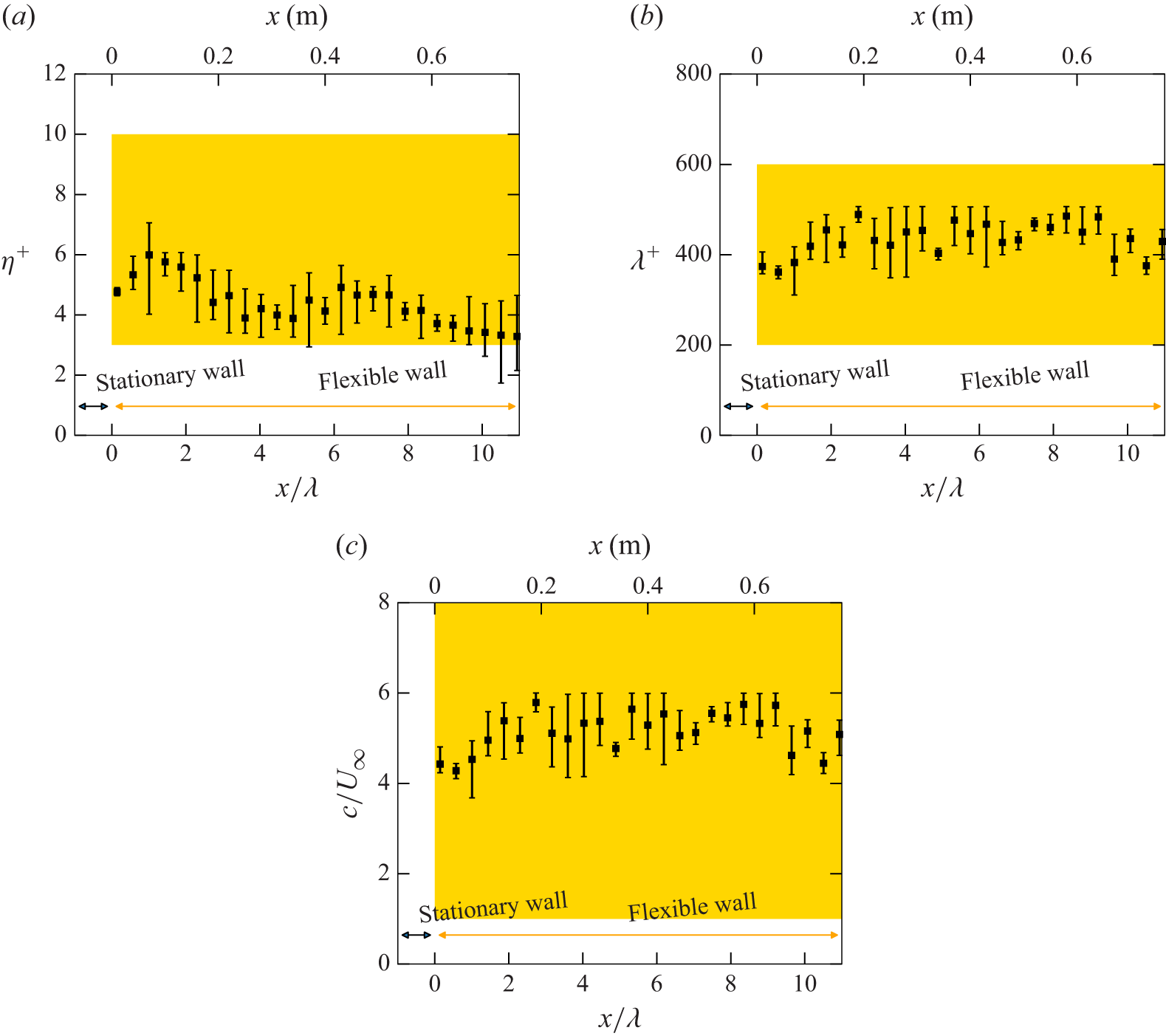
Streamwise distribution of travelling wave parameters: (a) amplitude; (b) wavelength; (c) wave speed. Error bars indicate coverage within
 $-200 \leq z^+ \leq 200$
. Areas in yellow indicate the occurrence of relaminarisation phenomena in turbulent channel flows (Nakanishi et al. Reference Nakanishi, Mamori and Fukagata2012; Mamori et al. Reference Mamori, Iwamoto and Murata2014).

Figure 3 shows the streamwise trend of fundamental wave parameters, the amplitude
 $\eta$
, the streamwise wavelength
 $\lambda$
and the streamwise wave speed
 $c$
, which are known to influence the drag-reduction effect (Nakanishi et al. Reference Nakanishi, Mamori and Fukagata2012; Mamori et al. Reference Mamori, Iwamoto and Murata2014). The amplitude and the streamwise wavelength are normalised in wall units at
 $x=0$
, and the streamwise wave speed is normalised by the free-stream velocity. These plots and error bars indicate the spanwise mean and spanwise coverage, respectively, within the range of
 $-200 \lesssim z^+ \lesssim 200$
. Figure 3(a) shows the amplitudes of the Fourier component at the oscillation frequency. The amplitudes of the other Fourier components were confirmed to be less than approximately 1 % of the amplitude at the oscillating frequency
 $f$
. The streamwise wavelengths in figure 3(b) are calculated such that
 \begin{equation} \lambda = \frac {2\pi }{\partial {\phi }/\partial {x}}, \end{equation}
where
 $\phi$
is a phase of the travelling wave following the definition in (1.2), in quasi-instantaneous wall deformations shown in figure 2. The wave speeds in figure 3(c) are calculated as
 $c = \lambda f$
. The highlighted areas in figure 3 exhibit each parameter’s effective range for relaminarisation phenomena (Nakanishi et al. Reference Nakanishi, Mamori and Fukagata2012; Mamori et al. Reference Mamori, Iwamoto and Murata2014). Although quantities shown in figure 3 have variations in the streamwise and spanwise directions due to the spanwise wave mode observed in figure 2, their values are almost within the effective range for relaminarisation phenomena (Nakanishi et al. Reference Nakanishi, Mamori and Fukagata2012; Mamori et al. Reference Mamori, Iwamoto and Murata2014).
Since the wave properties are quite sensitive to the applied tension and fixing condition of the rubber sheet, the wave amplitude and wavelength vary within the ranges of
 $4 \lesssim \eta ^+ \lesssim 8$
and
 $300 \lesssim \lambda ^+ \lesssim 500$
, respectively, after the replacement of the rubber sheet. Although such variations can induce a difference in the magnitude of the turbulence-suppressing effect or drag-reduction effect, the reducing scenario remains consistent; i.e. the periodic flow due to the wavy-wall motion suppresses random velocity fluctuations, causing drag reduction. This consistency, observed across different rubber sheet set-ups in Yoshida et al. (Reference Yoshida, Nimura, Mitsuishi, Murata and Iwamoto2025), is attributed to the fact that the parameter ranges, despite their variations, generally fall within those identified as effective for fully developed turbulent pipe and channel flows (Nakanishi et al. Reference Nakanishi, Mamori and Fukagata2012; Mamori et al. Reference Mamori, Iwamoto and Murata2014; Koganezawa et al. Reference Koganezawa, Mitsuishi, Shimura, Iwamoto, Mamori and Murata2019).
2.2. Particle image velocimetry measurement
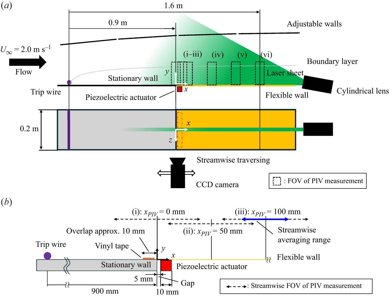
Schematic of experimental set-up (not to scale). (a) Entire test section. (b) Zoomed view around the oscillation source, i.e.
 $x=0$
. The FOVs of PIV measurements are numbered as (i)–(vi). The dot-dashed square in red in (a) indicates the glued area between the flexible wall and the piezoelectric actuator at the back side.

Figure 4 shows a schematic of the set-up for PIV measurements in the test section. The test section consists of a 1.0 m long entrance section made of a stationary acrylic plate and a 1.0 m long control section made of a flexible rubber sheet to generate a travelling wavy wall. To promote a rapid transition of the flow into turbulence, a trip wire with a diameter of 3 mm is placed 0.1 m downstream from the inlet. In this paper, the origin of the Cartesian coordinate system is located at the point on the wall at the downstream edge of the stationary wall, which is 5 mm upstream from the upstream edge of the piezoelectric actuator, as shown in figure 4(b), and at the spanwise centre of the wind tunnel. The turbulence intensity in the free stream is less than 1.0 %. The opposite side of the testing wall consists of four separate walls so that the pressure gradient in the free stream is adjusted to be negligible, and hence the streamwise variation of the free stream is within 0.2 %. We note that further details of this facility, e.g. rectification of inlet flow, are documented in Yoshida et al. (Reference Yoshida, Nimura, Mitsuishi, Murata and Iwamoto2025).
The measurements are performed at the spanwise centre (
 $z=0$
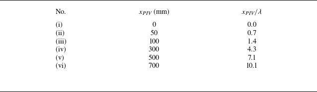
) of the wind tunnel in six streamwise locations, as numbered (i)–(vi) in figure 4, by traversing a CCD camera in the streamwise direction. In this paper, each measurement location is denoted by the streamwise centre of each field of view (FOV)
 $x_{\textit{PIV}}$
, as tabulated in table 1. Upstream, three measurement areas (i)–(iii) with overlaps are chosen to capture the immediate modification of the flow by the travelling wave, while downstream three areas (iv)–(vi) are separated by approximately 100 mm in the streamwise direction because the streamwise change due to the control is expected to be smaller than that upstream. A laser sheet generated by a Nd:YAG laser and a cylindrical lens is irradiated from the downstream end of the wind tunnel. In every streamwise location, the laser irradiation angle is optimised such that reflection from the wall is minimised, and the laser sheet thickness is adjusted to remove its streamwise variation by using the cylindrical lens, the focal length of which can be adjusted.
The PIV measurement locations. Here
 $x_{\textit{PIV}}$
represents the streamwise centre of each measurement area in figure 4.

A detailed configuration around upstream measurement areas (i)–(iii) and the wave generation mechanisms are illustrated in figure 4(b). The most upstream FOV (i) is at
 $x_{\textit{PIV}}=0$
, and consequently shifts 50 mm towards the streamwise direction by FOV (iii), such that they overlap 20 mm in each streamwise edge. We note that the PIV measurement at
 $x=0$
includes measurement over both the stationary and the wavy walls within FOV (i) to capture a sudden change in the wall configuration. Since the boundary condition at the interface between these two walls affects the wave and resultant flow characteristics, the applied tension on the rubber sheet in the overlapped region was fixed as in our previous study (Yoshida et al. Reference Yoshida, Nimura, Mitsuishi, Murata and Iwamoto2025). While the oscillation on the area glued to the piezoelectric actuator (dot-dashed square in red in figure 4
a) is a ‘standing wave’, the wave attains a ‘travelling’ characteristic by
 $x=20$
mm. The travelling wavy feature at
 $x=20$
mm was ensured because the streamwise phase lag
 $\partial {\phi }/\partial {x}$
in (2.1) between
 $x=10$
mm and
 $x=20$
mm was obtained, as shown in figure 3(b).
All experiments are carried out with free-stream velocity
 $U_\infty = 2.0$
m s−1. The Reynolds numbers based on the momentum thickness (
 $Re_\theta$
) and based on the friction velocity (
 $Re_\tau$
) are 620 and 220 at
 $x= 0.8$
m and 880 and 330 at
 $x = 1.6$
m, respectively. Seeding particles with a diameter of 1 μm are introduced by a Laskin-nozzle seeding generator (PIVpart14, PIVTEC GmbH), using silicone oil (DOS oil, Daihachi Chemical Industry Co. Ltd). The PIV measurements are performed at
 $x$
= 1.6 m with an area of 80 (streamwise)
 $\mathrm{\times }$
70 (wall-normal)
 $\mathrm{mm^2}$
, which corresponds to 510
 $\mathrm{\times }$
440 wall units, using a high-speed CCD camera with a resolution of 1280
 $\mathrm{\times }$
1024 px
 $^2$
. Velocities are obtained by spatial cross-correlation of seeded images with a window size of
 $32 \times 8\ \mathrm{px^2}$
with an overlap of 50 %, using PIV software (Koncerto II, Seika Digital Image Corp.). The recording rate is approximately 15 Hz with a pulse delay of 200 μs to obtain 2590 image pairs. To obtain multiple temporal-phase information from local measurement results, the trigger phase was intentionally shifted in successive runs to cover 10 different wave cycles. The phase was divided into 10 bins in the local measurement results, and more than 250 samples were collected for each bin. Convergence within a single bin was confirmed by an agreement within
 $\pm 2$
% in the wall-normal range of
 $y^+ \gtrsim 30$
between the first and the last halves in the 250 samples, although larger deviations up to 4 %–5 % are observed only in the vicinity of the wall. Phase-averaged statistics were then obtained by ensemble-averaging over the corresponding bin. The variance of the first and second moments across the 10 phase bins is below 1 % and 5 %, respectively.
(a,b) Map of mean velocity and RSS under the flat condition. (c,d) Streamwise average of mean velocity and RSS in each measurement area within one wavelength. Flat DNS profiles are adopted from the KTH database of Schlatter & Örlü (Reference Schlatter and Örlü2010).

Figure 5 shows the streamwise development of the mean velocity and the RSS profiles in the flat condition. Here, wall-normal location is normalized by
 $\delta_{99}^0$
, which is 99 % boundary layer thickness at
 $x=0$
. The coloured arrows in figures 5(a) and 5(b) indicate the streamwise ranges of averaging used in figures 5(c) and 5(d). In this paper, the superscript ‘+’ indicates normalisation based on
 $\nu$
and
 $u_\tau$
in each measurement area for the flat condition. The friction velocity
 $u_\tau$
was assumed by a stress balance profile, i.e.
 $\mathrm{d}{\bar {u}^+}/\mathrm{d}{y^+}-\overline {u^{\prime}v^{\prime+}}$
, and validated by agreement with previous direct numerical simulation (DNS) results (Schlatter & Örlü Reference Schlatter and Örlü2010) within 10 % at corresponding Reynolds numbers. Due to the uncertainty in the estimation of
 $u_\tau$
, statistics in figures 5(c) and 5(d) slightly deviate among the measurement locations. We note that the results for the wavy condition were nominally normalised using the same
 $u_\tau$
as in the flat case. An actual
 $u_\tau$
in the wavy condition is expected to be 3 % smaller than that in the flat case accompanied by the drag reduction (Yoshida et al. Reference Yoshida, Nimura, Mitsuishi, Murata and Iwamoto2025), whereas the main focus of the present study is direct comparison between flat and wavy conditions. The range of streamwise averaging was chosen to match the wavelength of the travelling wave, thereby minimising bias due to streamwise variations in amplitude. The local 99 % boundary-layer thickness was estimated using a diagnostic plot method, as proposed by Alfredsson, Segalini & Örlü (Reference Alfredsson, Segalini and Örlü2011) and Vinuesa et al. (Reference Vinuesa, Bobke, Örlü and Schlatter2016).
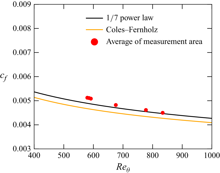
Figure 6 shows the development of the friction coefficient
 $c_f$
, based on the estimated friction velocity in each measurement area, i.e.
 $c_f = 2 u_\tau ^2 /U_\infty ^2$
, plotted against the Reynolds number based on momentum thickness
 $Re_\theta$
. The development supports the assumption of a zero pressure gradient in the wind tunnel, as the measurement results agree with estimation from the 1/7 power law,
 \begin{equation} c_f = 0.024 Re_\theta ^{-1/4}, \end{equation}
within a deviation of
 $\pm 5$
%. Because the Reynolds number of the present study is low, the deviation from the Coles–Fernholz relation (Fernholz & Finley Reference Fernholz and Finley1996)
 \begin{equation} \sqrt {\frac {2}{c_f}} = \frac {1}{\kappa } \ln (Re_\theta ) + C, \end{equation}
with constants
 $\kappa =0.384$
and
 $C=4.12$
, is relatively larger than the 1/7 law.
Flow development in the flat condition compared to the
 $1/7$
power law and the empirical formula by Fernholz & Finley (Reference Fernholz and Finley1996).

3. Results
3.1. Mean flow and Reynolds shear stress
Change of mean velocity due to control
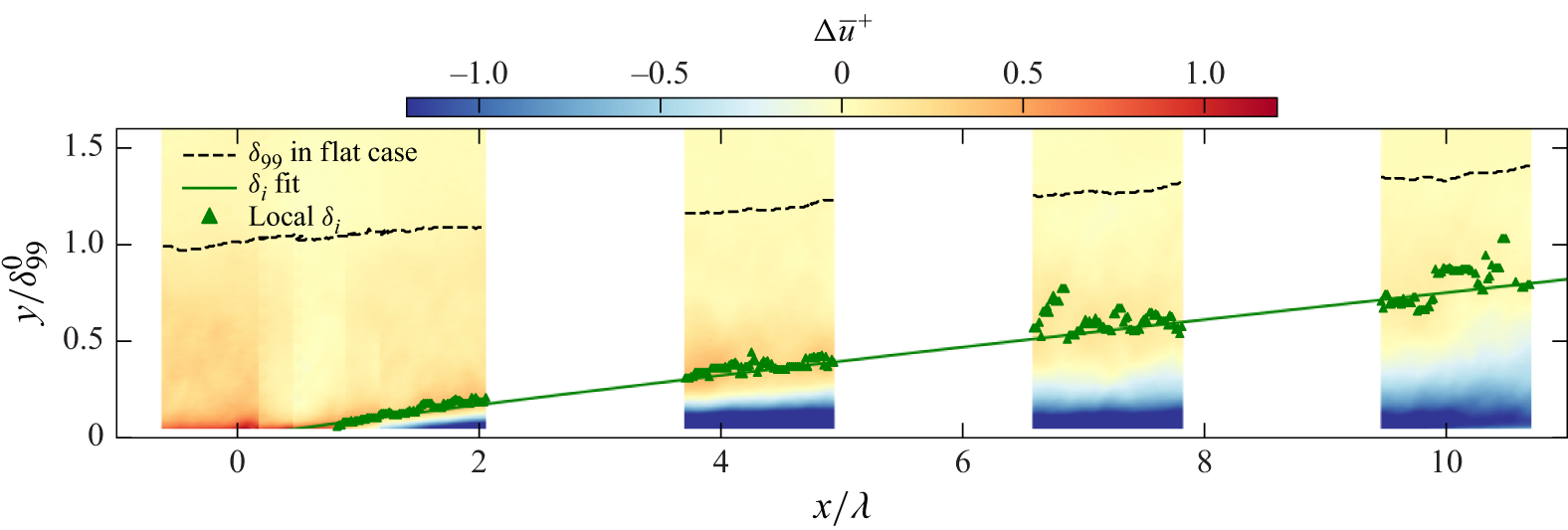
 $\Delta \bar {u}^+ = \bar {u}^{^+,{wavy}}- \bar {u}^{^+,{flat}}$
. Plots indicate local IBL thickness as wall-normal peaks of
 $\Delta \bar {u}^+$
, and its fitted line according to (1.4) is shown as a solid line.

Figure 7 shows the local change of the mean velocity
 $\Delta \bar {u}$
due to the control, where
 $\Delta f$
denotes local change of given variables
 $f$
due to the control, i.e.
 $\Delta f = f^{{wavy}} - f^{{flat}}$
. We note that the slight discontinuity in the streamwise profiles between FOVs (i)–(iii) (
 $0 \lesssim x/\lambda \lesssim 1$
) arises from the averaging performed in the overlapping edge regions of the FOVs, as illustrated in figure 4(b). A response often associated with drag-reduced flows, namely a reduction of mean velocity in the near-wall region and an increase in the outer region, is observed across the measurement area. The near-wall velocity reduction is attributed to the periodic flow induced by wall deformation, as reported in previous studies (Taneda & Tomonari Reference Taneda and Tomonari1974; Shen et al. Reference Shen, Zhang, Yue and Triantafyllou2003; Koganezawa et al. Reference Koganezawa, Mitsuishi, Shimura, Iwamoto, Mamori and Murata2019; Yoshida et al. Reference Yoshida, Nimura, Mitsuishi, Murata and Iwamoto2025). Characteristic periodic streamline patterns, initiated by the wavy wall moving upward and terminating in the wavy wall moving downward, produce a negative mean velocity near the crest of the wavy wall. As the flow develops downstream, the region of negative
 $\Delta \bar {u}$
expands in the wall-normal direction until approximately
 $x/\lambda \approx 4$
, after which its vertical extent remains nearly constant. This trend suggests that the periodic flow pattern establishes over a streamwise distance of
 $x/\lambda \approx 4$
, and a difference in physical features between
 $x/\lambda \lesssim 2$
and
 $x/\lambda \gtrsim 4$
.
To quantify the development of the outer-region increase in
 $\Delta \bar {u}$
, we adopt an IBL interpretation and define an IBL thickness
 $\delta _{{i}} (x)$
as the wall-normal location of the local peak in
 $\Delta \bar {u}$
. Following previous studies of IBL (Antonia & Luxton Reference Antonia and Luxton1971; Smits & Wood Reference Smits and Wood1985; Lee Reference Lee2015; Hanson & Ganapathisubramani Reference Hanson and Ganapathisubramani2016; Li et al. Reference Li, de Silva, Chung, Pullin, Marusic and Hutchins2022), the streamwise development of
 $\delta _{{i}}$
is shown together with a power-law fit given by (1.4), as a guide to the eye. In a similar manner, an IBL of
 $\Delta u^{\prime\prime}_{{rms}}$
and
 $\Delta (-\overline {u^{\prime\prime}v^{\prime\prime}})$
will be extracted later in figures 11 and 10, respectively, while we note that the multiple definitions of
 $\delta _{{i}}$
are proposed to extract characteristic features in each quantity. Namely,
 $\delta _{{i}}$
is defined by a wall-normal extremum for
 $\Delta \bar {u}$
and
 $\Delta u^{\prime\prime}_{{rms}}$
, and by a threshold criterion for
 $\Delta (-\overline {u^{\prime\prime}v^{\prime\prime}})$
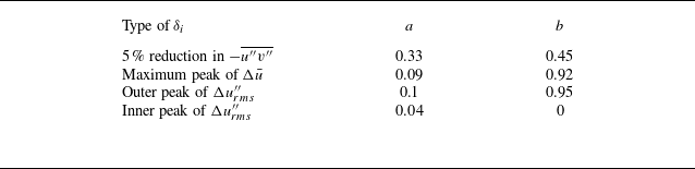
. The streamwise development of IBLs is summarised later in figure 13 and table 2 lists their growth rates.
Obtained coefficient
 $a$
and exponent
 $b$
for each
 $\delta _{{i}}$
.

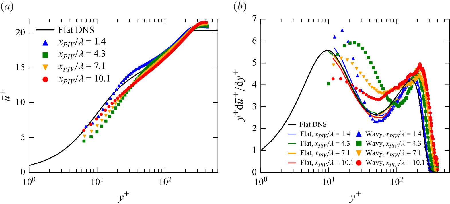
Mean velocity profiles (a) and profiles of diagnostic function (b). Plots are averaged in the streamwise direction in each measurement area within one wavelength. Flat DNS profiles are adopted from the KTH database of Schlatter & Örlü (Reference Schlatter and Örlü2010).

Figure 8(a) shows the mean velocity profiles at FOVs (iii)–(vi) over the travelling wavy wall. Each profile is obtained by averaging over one wavelength in the streamwise direction, following the same procedure used in figure 5. At
 $x_{\textit{PIV}}/\lambda = 1.4$
, the velocity in the range
 $20 \lesssim y^+ \lesssim 100$
is increased by approximately 0.3 in wall units compared with the flat-wall case. Here, despite the mean velocity increasing, the slope of the mean velocity profile apparently remains close to that of the flat-wall case upstream (
 $x_{\textit{PIV}}/\lambda \approx 1.4$
). To support the discussion of the local-slope behaviour of the mean profile, the diagnostic function
 $y^+ \mathrm{d}\bar {u}^+/\mathrm{d}y^+$
is plotted in figure 8(b). For the flat-wall case, the diagnostic function agrees well with the DNS results of Schlatter & Örlü (Reference Schlatter and Örlü2010), showing a local minimum at
 $y^+\approx 60$
, often associated with the von Kármán constant in canonical turbulent boundary layers. We note that the present Reynolds number is relatively low, and the logarithmic region is therefore not fully developed. Hence, the diagnostic function is used here only as a qualitative indicator of the local slope of the mean profile. At
 $x_{\textit{PIV}}/\lambda = 1.4$
, the wall-normal location and magnitude of the local minimum remain similar to those of the flat-wall case, while at downstream locations with
 $x_{\textit{PIV}}/\lambda \geq 4.3$
the minimum value increases. This streamwise trend in the local minimum of the diagnostic function supports the view that the mechanism responsible for modifying the mean velocity profile differs between
 $x_{\textit{PIV}}/\lambda = 1.4$
and the farther downstream region with
 $x_{\textit{PIV}}/\lambda \ge 4.3$
. The increase in the local minimum is consistent with a reduction in the turbulent momentum transfer, which is shown later as a reduction in the random RSS in figures 9 and 10.
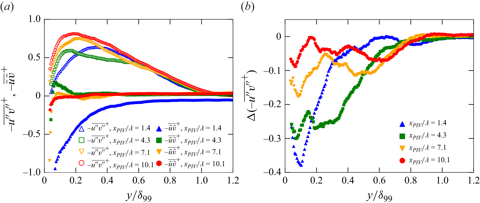
(a) Streamwise average of random and periodic RSSs in each measurement area within one wavelength for the wavy condition. (b) Change of random RSS due to travelling wavy wall (negative value indicates reduction in RSS). We note that
 $\Delta (-{\overline {\tilde {u}\tilde {v}}})$
is not shown in (b) because it is equivalent to
 $- \overline {\tilde {u}\tilde {v}}$
in (a).

Change of random RSS due to control
 $\Delta (-\overline {u^{\prime\prime}v^{\prime\prime}}^+) = -\overline {u^{\prime\prime}v^{\prime\prime}}^{+, {wavy}}- (-\overline {u^{\prime\prime}v^{\prime\prime}}^{+, {flat}})$
. Plots indicate local IBL thickness as the first height that indicates 5 % reduction looking down from the 99 % boundary-layer thickness, and its fitted line according to (1.4) is shown as a solid line.

Figure 9 shows the evolution of the RSS, decomposed into random and periodic components. In figure 9(a), the periodic RSS (denoted as
 $-\overline {\tilde {u}\tilde {v}}$
) and random RSS (denoted as
 $-\overline {u^{\prime\prime}v^{\prime\prime}}$
) are shown separately at FOVs (iii)–(vi). The random component decreases consistently at all locations, as summarised in figure 9(b), while the periodic component exhibits significant variation between
 $x_{\textit{PIV}}/\lambda = 1.4$
and other downstream locations. The periodic RSS at
 $x_{\textit{PIV}}/\lambda = 1.4$
exhibits a pronounced negative value extending up to
 $y/\delta _{99} \lesssim 0.4$
, attributed to the sudden change in the wall configuration, and even remains negative beyond the boundary-layer edge. This negative RSS may be related to a pumping effect because previous studies (Nakanishi et al. Reference Nakanishi, Mamori and Fukagata2012; Nabae et al. Reference Nabae, Kawai and Fukagata2020) have considered the negative periodic RSS as a peristaltic pumping effect driven by wall motion (Hœpffner & Fukagata Reference Hœpffner and Fukagata2009). Since the observation of the temporal evolution of the periodic RSS in streamwise-periodic turbulent flows (Nakanishi et al. Reference Nakanishi, Mamori and Fukagata2012; Nabae et al. Reference Nabae, Kawai and Fukagata2020) is absent, it is unclear whether the occurrence of negative periodic RSS is a phenomenon only in the turbulent boundary-layer flow; however, it is considered a transient response in the early stages of control. Meanwhile, the periodic RSS at
 $x_{\textit{PIV}}/\lambda \geq 4.3$
is limited to the wall-normal range of
 $y/\delta _{99} \lesssim 0.2$
, and those farther from the wall are almost zero. This behaviour is consistent with that of streamwise-periodic turbulent flows (Nakanishi et al. Reference Nakanishi, Mamori and Fukagata2012; Nabae et al. Reference Nabae, Kawai and Fukagata2020), in which the non-zero periodic RSS near the wall and the suppression of the random RSS away from the wall were interpreted as the direct effect and the turbulence-suppression effect due to the control, respectively. Namely, the present periodic RSS suggests a shift in the flow modification mechanism between
 $x_{\textit{PIV}}/\lambda = 1.4$
and
 $4.3$
, from the sudden application of the wavy actuation to the turbulence suppression farther downstream, which is consistent with the streamwise evolution of the mean velocity profile shown in figures 7 and 8.
The contrasting modifications in the mean velocity profile between the upstream (
 $x/\lambda \lesssim 2$
) and the downstream (
 $x/\lambda \gtrsim 4$
) regions are summarised in figures 7–9. In the upstream region, flow in the near-wall region rapidly responds to the change in the wall configuration from flat to wavy, while the underlying mechanisms in the outer layers remain unchanged. In the downstream region, however, the modification arises from the suppression of turbulent momentum transfer, as reflected in the reduction of the random RSS. The diagnostic function further supports the progressive influence of the travelling wave control on the local-slope indicator, which may represent a reduction in the nominal eddy viscosity.
3.2. Streamwise trend of turbulence suppression
Figure 10 illustrates the local change of the random RSS
 $-\overline {u^{\prime\prime}v^{\prime\prime}}^+$
induced by the travelling wave. The random RSS is slightly increased in
 $y/\delta _{99}^{0} \lesssim 0.2$
by
 $x/\lambda \lesssim 1$
, followed by a noticeable suppression in
 $y/\delta _{99}^{0} \lesssim 0.3$
by
 $x/\lambda \approx 2$
. Above this wall-normal location (
 $y/\delta _{99}^{0} \gtrsim 0.5$
), the profiles remain similar to those of the uncontrolled case, indicating that the outer-layer turbulence remains mostly unaffected by this streamwise location. Farther downstream, the reduction spreads in the wall-normal direction, indicating a delayed yet progressive influence on the outer layer. To indicate this gradual modification, the first height that indicates 5 % reduction looking down from the 99 % boundary-layer thickness is plotted as
 $\delta _{{i}}$
. In the same manner as in figure 7, the fitting curve of
 $\delta _{{i}}$
to (1.4) is shown to support discussion over the framework of the IBL. Although the reduction area in random RSS expands rapidly in the wall-normal direction by
 $x/\lambda \approx 2$
, the turbulent structures in the outer region are unchanged by the control, as suggested by the behaviour of the diagnostic function in figure 8. The streamwise lag in the change of the diagnostic function between
 $x/\lambda \lesssim 2$
and
 $x/\lambda \gtrsim 4$
suggests that the distance of
 $x/\lambda \approx 4$
is required to modify the mean velocity profile as a consequence of the reduction in the random RSS, whereas the initial response associated with the periodic component is reflected more rapidly, primarily as an upward shift of the mean velocity profile with only a minor change in the diagnostic function.
Change of streamwise random velocity fluctuation
 $\Delta u^{\prime \prime +}_{{rms}} = u^{\prime \prime +, {wavy}}_{{rms}}- u^{\prime \prime +, {flat}}_{{rms}}$
. Plots indicate local IBL thickness as inner and outer wall-normal minima of
 $u^{\prime \prime +}_{{rms}}$
, and its fitting according to (1.4) is shown as lines.

Figure 11 illustrates the streamwise development of the root-mean-square value of streamwise random velocity fluctuation
 $\Delta u^{\prime \prime +}_{{rms}}$
in the same manner as in figure 10. The change in
 $u^{\prime \prime +}_{{rms}}$
is negligible up to
 $x/\lambda \approx 1$
and becomes significant further downstream. At upstream locations (
 $1 \lesssim x/\lambda \lesssim 2$
), the reduction in the fluctuation is primarily confined to the near-wall region (
 $y/\delta _{99} \lt 0.3$
). Farther downstream (
 $x/\lambda \gtrsim 4$
), the reduction of the fluctuations is found even in
 $y/\delta _{99} \gt 0.5$
, suggesting that the control effect gradually penetrates outward from the wall as the flow develops. The separated reduction areas of
 $\Delta u^{\prime\prime}_{{rms}}$
in near-wall and outer regions are characterised by
 $\delta _{{i}}$
of each minima. In the same manner as in figures 7 and 10, fitting curves of
 $\delta _{{i}}$
to (1.4) of their minima are shown to support discussion over the framework of the IBL. In those downstream locations after
 $x/\lambda \approx 4$
, a slight increase is found between the near-wall and outer reductions. This increased fluctuation is due to the shift of the wall-normal peak location of
 $u^{\prime \prime +}_{{rms}}$
from
 $y^+ = 15$
towards
 $y^+ = 20$
–
 $30$
in the wavy condition. Although the peak value of
 $u^{\prime\prime+}_{{rms}}(y)$
is reduced at all streamwise stations, the near-wall peak becomes broader and flatter, as its peak location shifts from
 $y^{+}\approx 15$
to
 $y^{+}\approx 20$
–
 $30$
. This broadening results in locally larger
 $u^{\prime\prime+}_{{rms}}$
in the range
 $0.1\lesssim y/\delta _{99}\lesssim 0.5$
compared with the flat-wall case. Since
 $u_{{rms}}^{\prime \prime +}$
in the near-wall region is associated with the near-wall streaks, a more detailed examination is provided in § 3.3. A noteworthy reduction trend in
 $u^{\prime \prime +}_{{rms}}$
here is that the effect is confined near the wall immediately after the onset of control and subsequently spreads wall-normally downstream.
Change of production term in the random Reynolds stress budget equation for the streamwise random velocity fluctuation due to control
 $\Delta P^{\prime\prime+}_{11} = P^{\prime\prime+, wavy}_{11} - P^{\prime\prime+,flat}_{11}$
.

To explain the cause of the increase in
 $u^{\prime\prime}_{{rms}}$
in
 $0.1 \lesssim y/\delta _{99}^0 \lesssim 0.5$
and
 $4.3 \leq x_{\textit{PIV}}/\lambda \leq 10.1$
(FOVs (iv)–(vi)), a random Reynolds stress budget of the governing equation of random velocity fluctuations (Touber & Leschziner Reference Touber and Leschziner2012) was utilised. Production terms for the random velocities are written as
 \begin{equation} P^{\prime\prime}_{ij} = - \overline {u^{\prime\prime}_j u^{\prime\prime}_k} \frac {\partial \bar {u}_i}{\partial x_k} - \overline {u^{\prime\prime}_i u^{\prime\prime}_k} \frac {\partial \bar {u}_j}{\partial x_k} - \overline {\langle u^{\prime\prime}_j u^{\prime\prime}_k \rangle \frac {\partial \tilde {u}_i}{\partial x_k}} - \overline {\langle u^{\prime\prime}_i u^{\prime\prime}_k \rangle \frac {\partial \tilde {u}_j}{\partial x_k}} ,\\ \end{equation}
where the angle brackets denote phase-averaged quantities. In the case of
 $i=j=1$
, which indicates the production term in the Reynolds stress budgets of
 $\overline {u^{\prime\prime}u^{\prime\prime}}$
(
 $u^{\prime\prime}_{{rms}}$
squared), the production term was calculated within our measurement results as follows:
 \begin{equation} P^{\prime\prime}_{11} \approx - 2 \overline {u^{\prime\prime} v^{\prime\prime}} \frac {\partial \bar {u}}{\partial y}. \end{equation}
Figure 12 shows the streamwise development of the random production in the same manner as in figure 11. In the streamwise location immediately downstream of the actuation point, up to approximately
 $x/\lambda \approx 2$
, the reduction in random production is predominantly found in the near-wall region (
 $y/\delta_{99}^{0} \lesssim 0.1$
). Further downstream, in the range
 $4 \lesssim x/\lambda \lesssim 8$
, a reduction in random production additionally appears in the region further from the wall. This streamwise delayed response in the outer region from the near-wall region indicates gradual modification of the flow, as indicated in figures 7–10. Namely, the direct effect in the near-wall region secondarily alters the turbulent feature in the outer region along with the streamwise development of the flow. Concurrently, an increase in the random production is also observed in the wall-normal range
 $0.1 \lesssim y/\delta_{99}^{0} \lesssim 0.5$
in the same streamwise locations (
 $4 \lesssim x/\lambda \lesssim 11$
). The random production was increased in the intermittent region because of the increase in wall-normal velocity gradient (see figure 8
b) in the corresponding region, although the random RSS (see figure 10) was reduced. This observed trend is similar to that of the streamwise random root-mean-square velocity fluctuations (
 $u^{\prime\prime}_{{rms}}$
), as depicted in figure 11. Considering the budget equation of streamwise Reynolds normal stress, where the random production is a key contributor to
 $\overline {u^{\prime\prime}u^{\prime\prime}}$
, the observed modifications in
 $u^{\prime\prime}_{{rms}}$
can be attributed to the change in the random production.
(a) Streamwise development of 99 % boundary-layer thickness
 $\delta _{99}$
and IBL thickness
 $\delta _{{i}}$
. Symbols and lines indicate streamwise average of measurement result within one wavelength and the fitting result according to (1.4), respectively. (b) Physical interpretation of the streamwise development of various thicknesses in (a).

Figure 13 summarises the streamwise development of IBLs in figures 7, 11 and 10 for comparison. Figure 13(a) shows the estimated
 $\delta _{{i}}$
for each quantity plotted against the streamwise distance
 $x/\lambda$
on a log–log scale, along with the fitting results based on (1.4). All datasets align well with the fitting lines, suggesting that the development of these characteristic heights can be effectively modelled by the power-law relationship in (1.4). The obtained
 $a$
and
 $b$
are tabulated in table 2 to facilitate comparison of the growth rate of
 $\delta _{{i}}$
with previous IBL studies. Here, the exponents for the outer-layer-based definitions are of order
 $b \approx$
0.9–1.0, which are comparable with the rough-wall IBL exponents reported in Rouhi, Chung & Hutchins (Reference Rouhi, Chung and Hutchins2019).
A noteworthy feature in figure 13(a) is that the slopes
 $a$
or growth exponents
 $b$
in (1.4) appear to differ among the various quantities. This observation suggests that the control effect propagates through the boundary layer via mechanisms with different characteristic speeds, resulting in a multilayered structure of modification, as schematically illustrated in figure 13(b). No growth is observed in
 $\delta _{{i}}$
based on the minimum value of
 $\Delta u^{\prime\prime}_{{rms}}$
, which might correspond to a direct, local effect of the wall forcing, confined to a very thin layer near the wall. The direct effect of the travelling wave has often been deduced from the periodic component in (1.3) (Nakanishi et al. Reference Nakanishi, Mamori and Fukagata2012; Mamori et al. Reference Mamori, Iwamoto and Murata2014; Yoshida et al. Reference Yoshida, Nimura, Mitsuishi, Murata and Iwamoto2025), whereas the present observation elucidates the direct effect even in the random component. The regions of
 $(-\overline {u^{\prime\prime}v^{\prime\prime}})$
reduction seem to expand most rapidly. This rapid development could be interpreted as the propagation of the primary turbulence-suppression effect in the near-wall region, followed by a secondary modification in the outer region. The development of
 $\delta _{{i}}$
based on the maximum peak of
 $\Delta \bar {u}$
and the outer minimum in
 $\Delta u^{\prime\prime}_{{rms}}$
may also indicate the secondary response, consequent of the near-wall modifications gradually influencing the larger-scale structures farther from the wall. The similar growth rates of these two IBLs among
 $\Delta \bar {u}$
and
 $\Delta u^{\prime\prime}_{{rms}}$
suggest a concurrent modification of outer-layer large-scale motions. This interpretation is consistent with the gradual response of the wall-normal location of the local minimum of the diagnostic function
 $y\,\mathrm{d}{u}/\mathrm{d}{y}$
in figure 8(b), indicating a reduction in the eddy viscosity by the preceding reduction of the random RSS. While the observed sequence of events suggests a plausible causal relationship, we acknowledge that the different definitions of
 $\delta _{{i}}$
call for a cautious interpretation. Hence, we cannot draw a definitive conclusion on the causal relation from the present analysis alone. Nevertheless, the clear distinction in the development trends provides valuable insight into the complex, spatially evolving nature of the flow modification induced by the travelling wave control.
Now we compare the distance in the present study with the time to converge the drag-reduction effect in previous DNS studies in fully developed internal flows (Nakanishi et al. Reference Nakanishi, Mamori and Fukagata2012; Mamori et al. Reference Mamori, Iwamoto and Murata2014; Koganezawa et al. Reference Koganezawa, Mitsuishi, Shimura, Iwamoto, Mamori and Murata2019; Nabae et al. Reference Nabae, Kawai and Fukagata2020). As these prior studies were conducted in temporally evolving domains, the streamwise distance in the present set-up was converted into an equivalent time scale using the convective velocity of near-wall turbulence:
 \begin{equation} \mathcal{T} = \frac {L}{u_c}, \end{equation}
where
 $L$
is the streamwise distance and
 $u_c$
is the convective velocity of the near-wall turbulence, taken as
 $10 u_\tau$
based on Kim & Hussain (Reference Kim and Hussain1993). This approach follows the methodology of Skote (Reference Skote2012), who demonstrated that the spatial development of the drag-reduction effect via spanwise wall oscillation can be equivalently interpreted as a temporal evolution using this convective scaling. The number of wave cycles experienced over the duration
 $\mathcal{T}$
obtained by (3.3) was estimated as
 \begin{equation} N = f \mathcal{T}, \end{equation}
where
 $f$
is the wave frequency. According to previous DNS studies (Nakanishi et al. Reference Nakanishi, Mamori and Fukagata2012; Mamori et al. Reference Mamori, Iwamoto and Murata2014; Koganezawa et al. Reference Koganezawa, Mitsuishi, Shimura, Iwamoto, Mamori and Murata2019; Nabae et al. Reference Nabae, Kawai and Fukagata2020), a stable drag-reduction effect emerges after approximately 100–800 wave cycles. In the present measurements, the estimated number of wave cycles at
 $x/\lambda = 10$
is about 120, which slightly exceeds the lower bound of the reported range. Extrapolation in the streamwise direction in figure 13(a) supports the discussion using the experienced wavenumber defined in (3.4). For example, fitting lines of
 $\delta _{{i}}$
for the maximum peak of
 $\Delta \bar {u}$
and the minimum peak of
 $\Delta u^{\prime\prime}_{{rms}}$
can exceed
 $\delta _{99}$
in
 $x/\lambda \approx 30$
, which is approximately equivalent to 300 wave cycles being experienced. We can assume that the flow reaches equilibrium after
 $\delta _{{i}}$
becomes as thick as
 $\delta _{99}$
, and that the estimated location (
 $x/\lambda \approx 30$
) based on the power fitting by (1.4) agrees with
 $N$
in previous studies of internal flows.
3.3. Flow structure
The fluctuating energy at the wall-normal peak of
 $u^{\prime\prime}_{{rms}}$
for flat-wall turbulence is known to be comprised of a streaky structure, whose representative streamwise length scale is approximately 1000 wall units (Robinson Reference Robinson1991). Such streamwise long features in the near-wall region play a significant role in maintaining turbulence of the boundary layer, as they can be characterised by turbulent statistics, e.g. the profile of mean velocity and the RSS. Characteristics of streaky structures in drag-reduced flows are of great interest because they indicate the structural feature in the near-wall region, as they affect turbulent statistics in the outer regions. To extract time-averaged structural features, we utilise the two-point correlation coefficient, which is defined as
 \begin{equation} \overline{R_{u^{\prime\prime}u^{\prime\prime}} (\Delta x, y_{\textit{ref}}, y)} = \frac{\overline{u^{\prime\prime}(x, y_{\textit{ref}}) u^{\prime\prime}(x + \Delta x, y)}}{\sqrt{\overline{u^{\prime\prime2}} (y_{\textit{ref}})} \sqrt{\overline{u^{\prime\prime2}} (y)}}, \end{equation}
where
 $\Delta x$
is the spatial separation in the streamwise direction and
 $y_{{ref}}$
is the wall-normal reference location. A motivation in this section is to reveal the modification of the streaky structure depicted by (3.5) due to the travelling wave.
(a–c) Maps of time-averaged two-point correlations of the streamwise random velocity fluctuations with reference wall-normal location of
 $y_{{ref}}^+=15$
and (d) plot on
 $y_{{ref}}^+$
. Maps of (a) flat condition at
 $x_{\textit{PIV}}/\lambda = 1.4$
, (b) wavy condition at
 $x_{\textit{PIV}}/\lambda = 1.4$
and (c) average of wavy condition at
 $x_{\textit{PIV}}/\lambda = 4.3$
, 7.1 and 10.1. Dot-dashed lines in white in (a–c) indicate
 $y_{{ref}}^+=15$
and dashed lines in black in (a–d) indicate
 $\overline {R_{u^{\prime\prime}u^{\prime\prime}}} = 0.2$
to clarify the streak core region.

Figures 14(a)–14(c) show maps of the streamwise two-point correlation of the streamwise random velocity fluctuations at the flat wall, at
 $x_{\textit{PIV}}/\lambda = 1.4$
(FOV (iii)) and at the downstream region
 $x_{\textit{PIV}}/\lambda \geq 4.3$
(FOVs (iv)–(vi)), respectively. In figure 14(c), the downstream correlation map is obtained as the average over the three downstream stations at
 $x_{\textit{PIV}}/\lambda = 4.3$
, 7.1 and 10.1. These three stations are presented as their average since no significant differences are observed among them, as indicated by the narrow shaded band representing their variance in figure 14(d). Here, the region that satisfies
 $R_{\overline {u^{\prime\prime}u^{\prime\prime}}} \ \gt \ 0.2$
is highlighted by the dashed lines to indicate the core of the near-wall streaks. There is a decrease in the spatial scales of the core region in the wavy conditions shown in figure 14(b,c) compared with the flat condition in figure 14(a), indicating that the near-wall streaks are weakened by the travelling wave control. A distinctive feature of the core of
 $R_{\overline {u^{\prime\prime}u^{\prime\prime}}} \ \gt \ 0.2$
in figure 14(b) is the elongated feature downstream towards
 $\Delta x^+ \approx 400$
and the tiny region upstream at
 $\Delta x^+ \approx - 400$
that is distant from the main part around
 $\Delta x^+ = 0$
. Meanwhile, in figure 14(c), such a unique feature is not indicated; however, overall correlations are reduced compared with the flat case in figure 14(a). Those differences are summarised in figure 14(d), which shows the two-point correlation coefficients with
 $y_{{ref}}^+ = 15$
(the white dot-dashed line in figure 14
a–c). Although the shape of the correlation for
 $x_{\textit{PIV}}/\lambda \geq 4.3$
is similar to the case of the flat wall, those for
 $x_{\textit{PIV}}/\lambda = 1.4$
indicate minima in
 $\Delta x^+ \approx \pm 200$
, and they recover towards
 $\Delta x^+ \approx \pm 400$
. As we considered that the wavelength of the travelling wave is approximately 440 in wall units (see figure 3
b), the correlation in
 $x_{\textit{PIV}}/\lambda = 1.4$
is substantially affected by the travelling wave, while such a trend is not observed for
 $x_{\textit{PIV}}/\lambda \geq 4.3$
.
Although a reduction in the spatial extent of the near-wall streaky structure does not always lead to a suppression of turbulent fluctuations and a subsequent drag reduction, we argue that this is the case in the present configuration. Previous studies of flows over steady wavy walls (De Angelis, Lombardi & Banerjee Reference De Angelis, Lombardi and Banerjee1997; Cherukat et al. Reference Cherukat, Na, Hanratty and McLaughlin1998; Nakagawa & Hanratty Reference Nakagawa and Hanratty2001; Sun et al. Reference Sun, Zhu, Hu and Zhang2018) have reported increased turbulent fluctuations and drag, while the streamwise extent of near-wall streaks depends on the wavelength of the wavy wall. In particular, De Angelis et al. (Reference De Angelis, Lombardi and Banerjee1997) considered a wavy-wall channel with a wave height and steepness of
 $\eta ^+ = 8.5$
and
 $a/\lambda = 0.025$
, respectively, which are of the same order as for the present wall as indicated in figure 3 (
 $\eta ^+ \approx 5$
,
 $a/\lambda \approx 0.01$
). In the steady wall case (De Angelis et al. Reference De Angelis, Lombardi and Banerjee1997), the representative streamwise length scale of the near-wall streaks is synchronised with the wavelength, leading to increased drag due to enhanced turbulence intensities, which are attributed to flow separation at the wave crests. For travelling wavy walls, Shen et al. (Reference Shen, Zhang, Yue and Triantafyllou2003) showed that such separation is present when the wave speed is in the range
 $c/U_\infty \lt 1$
, whereas the separation is absent in travelling waves with a higher wave speed
 $c/U_\infty \geq 1$
, as in the present study, which are known to reduce drag. The contrasting behaviour at different wave speeds underlines the importance of parameter choice for achieving drag reduction (Nakanishi et al. Reference Nakanishi, Mamori and Fukagata2012; Mamori et al. Reference Mamori, Iwamoto and Murata2014; Nabae et al. Reference Nabae, Kawai and Fukagata2020). Moreover, artificial damping of turbulent fluctuations in the near-wall region is known to reduce drag and to be accompanied by turbulence suppression farther from the damping region (Iwamoto et al. Reference Iwamoto, Fukagata, Kasagi and Suzuki2005; Bannier, Garnier & Sagaut Reference Bannier, Garnier and Sagaut2016). Imposing such damping to decrease the streamwise coherence of the streaks has been shown to yield drag reduction while the turbulence itself is sustained (Jiménez & Pinelli Reference Jiménez and Pinelli1999; Jiménez Reference Jiménez2022). Based on this body of knowledge, together with the observed reduction in
 $u^{\prime\prime}_{ {rms}}$
and RSS, we interpret the drag reduction reported in Yoshida et al. (Reference Yoshida, Nimura, Mitsuishi, Murata and Iwamoto2025) as a consequence of reduced turbulent fluctuations associated with the shortening of the near-wall streaks shown in figure 14.
Phase-averaged two-point correlations of the streamwise random velocity fluctuations with reference wall-normal location of
 $y_{{ref}}^+=15$
at
 $x_{\textit{PIV}}/\lambda = 1.4$
(a–e) and average of
 $x_{\textit{PIV}}/\lambda \geq 4.3$
(f–j). Correlations in reference phase
 $\phi _{{ref}}/\pi$
of (a,f) 0.0, (b,g) 0.5, (c,h) 1.0 and (d,i) 1.5. Phase dependence of the correlation at
 $y_{{ref}}^+=15$
is summarised in (e,j). White cross in (a–d,f–i) and dot-dashed line in (e,j) indicate
 $\phi /\pi = \phi _{{ref}}/\pi$
. Dashed lines in black indicate
 $\langle R_{u^{\prime\prime}u^{\prime\prime}} \rangle = 0.2$
to clarify the streak core region.

Figure 15 shows the phase-averaged two-point correlation coefficients to confirm the geometrical relationship between the wave and the streaky structures, which is conjectured in figure 14. Figure 15(a–d,f–i) shows maps of the phase-averaged two-point correlation coefficients with four different reference phases
 $\phi _{{ref}}$
of the travelling wave as a reference location in the streamwise direction
 $x_{{ref}}$
defined as follows:
 \begin{equation} \langle R_{ u^{\prime\prime}u^{\prime\prime}} (\phi _{{ref}}, \phi , y_{{ref}}, y)\rangle = \frac {\langle u^{\prime\prime}(\phi _{{ref}}, y_{{ref}}) u^{\prime\prime}(\phi , y) \rangle } {\sqrt {\langle u^{\prime\prime2} (\phi _{{ref}}, y_{{ref}})\rangle } \sqrt {\langle u^{\prime\prime2} (\phi , y)\rangle }}. \end{equation}
In this paper, the wave is defined as (1.1) and, therefore, reference phases
 $\phi _{{ref}}/\pi =$
0.0, 0.5, 1.0 and 1.5 are the location of a crest, a leeward, a bottom and a windward, respectively. The correlation maps at
 $x_{\textit{PIV}}/\lambda =1.4$
(figure 15
a–d) show that the region of high correlation is interrupted across the wave crest, whereas downstream at
 $x_{\textit{PIV}}/\lambda \geq 4.3$
(figure 15
f–i) the maps become less dependent on
 $\phi _{{ref}}$
. Note that
 $\langle R_{u^{\prime\prime}u^{\prime\prime}}\rangle$
attains its maximum at the reference point (white cross) by definition, and therefore the peak at the crest in figure 15(a,f) reflects the choice of
 $\phi _{{ref}}/\pi =0.0$
. Specifically, at
 $x_{\textit{PIV}}/\lambda =1.4$
the crest acts as a geometric barrier that prevents correlated motions from extending continuously across the crest, while this interruption by the crest is much weaker at
 $x_{\textit{PIV}}/\lambda \geq 4.3$
. Figure 15(e,j) shows the phase-averaged correlation coefficient on the line of
 $y^+=15$
in all phases to summarise the trend. At
 $x_{\textit{PIV}}/\lambda = 1.4$
, the correlations in the wave crests (
 $\phi / \pi = 0$
or
 $2$
) are once reduced below
 $\langle R_{u^{\prime\prime}u^{\prime\prime}}\rangle = 0.1$
, and they recover slightly towards the distance from the reference point (
 $\phi _{{ref}}/\pi = \phi /\pi$
). This trend indicates that the streaky structures rarely straddle the wave crest and are often trapped within the wave bottom. Although the recovery of the correlation is not indicated in
 $x_{\textit{PIV}}/\lambda \geq 4.3$
, a slight effect of the wave crest is observed in the bound of
 $\langle R_{u^{\prime\prime}u^{\prime\prime}}\rangle = 0.2$
in the range
 $0 \leq \phi _{{ref}}/\pi \leq 1.0$
on the line of
 $\phi /\pi = 0$
, because the lower part of near-wall streaks rarely extend across the wave crest. A characteristic profile in
 $x_{\textit{PIV}}/\lambda = 1.4$
is exhibited in the horn-like profile of the bound of
 $\langle R_{u^{\prime\prime}u^{\prime\prime}}\rangle = 0.2$
for
 $\phi _{{ref}}/\pi \approx 1.5$
. This profile indicates the existence of residual streaky structures after leaping the wave crest that remain correlated between them. Hence, the typical near-wall streaks are modified at
 $x_{\textit{PIV}}/\lambda = 1.4$
, and they settle into their characteristic feature in the downstream region.
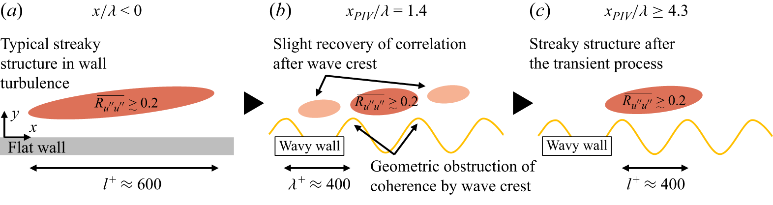
Conceptual illustration of the streamwise evolution of streaky structures subjected to travelling wave control. (a) Typical streaky structures in the upstream region before the control. (b) Transient process in an early stage of the control. (c) Farther downstream, resultant streamwise coherence of streaky structures is shortened due to the control.

To interpret the spatial evolution of the near-wall streaks under the influence of the travelling wave, we propose a conceptual model as illustrated in figure 16. This schematic is constructed based on the observed streamwise decorrelation in figure 14 and the phase-dependent coherence reduction in figure 15. At
 $x_{\textit{PIV}}/\lambda = 1.4$
, coherent streaks with streamwise lengths of approximately
 $l^+ \approx 1000$
persist in the absence of wall deformation. However, immediately downstream of the wave actuator (
 $x/\lambda \approx 1.4$
), the crest of the travelling wave geometrically disrupts the continuous correlation of streaks. This results in fragmented clusters of high- and low-speed flow that are weakly correlated across the wave crest, which is evidenced by the local minima in the streamwise two-point correlations and their dependence on wave phase. Farther downstream (
 $x_{\textit{PIV}}/\lambda \geq 4.3$
), the streaky structures simply indicate reduced streamwise coherence length, suggesting that a new equilibrium state emerges following the transient modulation by the travelling wave. An interesting feature here is that the reduction magnitude in fluctuating energy of
 $u^{\prime\prime}_{{rms}}$
in the buffer layer is almost constant in the streamwise direction, as shown in figures 11 and 13(a), while their spatial structures differ in the streamwise direction. A possible scenario can be drawn from this feature, as the travelling wave immediately reduces the near-wall fluctuating energy at
 $x_{\textit{PIV}}/\lambda = 1.4$
, and its spatial features become stable at
 $x_{\textit{PIV}}/\lambda \geq 4.3$
. This process may represent the suppression mechanism of turbulence and associated drag reduction observed for
 $x_{\textit{PIV}}/\lambda \geq 4.3$
.
4. Summary and conclusion
The streamwise evolution of turbulent boundary-layer flow over a travelling wavy-wall deformation was investigated using two-component PIV. A control was applied to the flow developing from
 $Re_\theta \approx 620$
and
 $Re_\tau \approx 250$
to
 $Re_\theta \approx 880$
and
 $Re_\tau \approx 330$
over a distance of 0.7 m, which is approximately equivalent to 11 times the wavelength of the travelling wave. Particle image velocimetry measurements were performed at several streamwise locations to observe the streamwise evolution process of turbulent characteristics due to the travelling wave control. Upstream, the region indicates the reduction in the turbulent fluctuations is limited in the near-wall region, while when the control is applied in the streamwise direction, the affected regions are spread in the wall-normal direction. At the downstream end of the measurement location, turbulence intensities are significantly reduced as in our previous study (Yoshida et al. Reference Yoshida, Nimura, Mitsuishi, Murata and Iwamoto2025), using the same travelling wave generation mechanisms, from which a drag-reduction effect is inferred.
The downstream evolution of the flow was interpreted within the framework of an IBL. The thickness
 $\delta _{{i}}$
, defined from several statistical indicators, follows a power-law growth with streamwise distance. Although the scaling exponent varied depending on the chosen indicator, the overall tendency suggests that the effect of wavy-wall forcing diffuses towards the edge of the boundary layer, except for
 $\delta _{{i}}$
based on near-wall reduction in random streamwise fluctuation
 $u^{\prime\prime}_{{rms}}$
. The IBL based on near-wall
 $u^{\prime\prime}_{{rms}}$
may represent a direct effect of the control, as it is constant in the streamwise direction, whereas other developing effects may represent a resultant modification of the turbulent structure across the boundary layer. This description provides a useful basis for comparing different wall-based control strategies in terms of their spatial development and effectiveness.
The turbulent characteristics in the downstream region offer distinctive features compared with the flat-wall turbulence. The reduction of
 $u^{\prime\prime}_{{rms}}$
is found where its production is reduced, thereby the production mechanisms in the wavy condition are modified into their specific characteristics. The behaviour of the mean profile in the region usually associated with the logarithmic layer is consistent with a reduced nominal eddy viscosity, as suggested by the diagnostic function
 $y\, \mathrm{d}{\bar {u}}/\mathrm{d}{y}$
. A streamwise lag in the change in the slope of log layer to outer layer is observed, implying that the turbulent features are gradually altered as the flow experiences the travelling wave control, consistent with the IBL analysis.
The near-wall streaks indicated by two-point correlations of the streamwise random velocity also show distinctive behaviour between the early stage of control and further-downstream locations. In the upstream region, the correlation decreases rapidly relative to the flat-wall case by
 $\Delta x/\lambda = \pm 0.5$
and recovers towards
 $\Delta x/\lambda = \pm 1.0$
, indicating that the streamwise length scale of the streaky structure is geometrically restricted by the crest of the travelling wave. Farther downstream, the streamwise coherence decreases without such a wave-dependent feature, suggesting that the initial interruption of the near-wall streaks is established as the flow experiences the travelling wave.
The present results provide an experimental observation of the transient process of fully developed turbulent boundary-layer flow, which exhibited a unique characteristic induced by the travelling wave. Further optimisation of the wave generation mechanism, particularly in terms of amplitude and frequency tuning, may enhance turbulence suppression and contribute to more effective drag-reduction strategies. Future work will refine these parameters and explore their impact in high-Reynolds-number flows.
Funding
This work was supported by JSPS KAKENHI grant numbers JP21H05007, JP21H01245 and JP24KJ1022.
Declaration of interests
The authors report no conflict of interest.