MODEL

The game begins with Nature selecting the Target’s military capability m ₂. Nature sets $$m_{2} =\underline {m}_{2} $$ with probability w, indicating the Target is relatively weak, and $m_{2} =\bar{m}_{2} $ with probability 1−w, indicating the Target is relatively strong, where $0\,\lt \,\underline {m}_{2} \,\lt \,\bar{m}_{2} $ . The Target then chooses whether or not to arm. If the Target arms, it incurs cost k>0, and its total military capabilities increase by α>0.

After observing the Target’s decision, the Challenger demands x∈[0,1], which the Target either accepts or rejects. If the Target accepts, the Challenger receives x whereas the Target receives either 1−x or 1−x−k, depending on whether the Target armed. If the Target rejects, a war occurs, which the Challenger wins with probability p. We assume the side that wins keeps the entire value of the good in dispute. Moreover, we assume each side incurs some loss of utility owing to the costs of war, denoted c ₁∈(0,1] and c ₂∈(0,1] for the Challenger and Target, respectively. In the event of war, the Challenger receives p(1)+(1−p)(0)−c ₁=p−c ₁ and the Target receives p(0)+(1−p)(1)−c ₂=1−p−c ₂ (or 1−p−c ₂−k, if the Target armed).

The precise value of p is a function of m ₁, m ₂, and, if the Target armed, α, where m ₁>0 is the Challenger’s military capability. If the Target is weak and did not arm, $$\vskip -1pt p={{m_{1} } \over {m_{1} {\plus}\underline {m}_{2} }}\,\equiv\,\bar{p}$$ . If the Target is weak and armed, $$p={{m_{1} } \over {m_{1} {\plus}\underline {m}_{2} {\plus}\alpha }}\,\equiv\,\hat{p}$$ . If the Target is strong and did not arm, $p={{m_{1} } \over {m_{1} {\plus}\bar{m}_{2} }}\,\equiv\,\tilde{p}$ . If the Target is strong and armed, $p={{m_{1} } \over {m_{1} {\plus}\bar{m}_{2} {\plus}\alpha }}\,\equiv\,\underline {p}$ . By assumption, α>0 and $\underline {m}_{2} \lt \bar{m}_{2} $ , therefore $\underline {p}$ must be the smallest value of p and $\bar{p}$ must be the largest.Footnote ³

Equilibria

As we assume the Challenger is uninformed about the Target’s type, we solve the model for perfect Bayesian equilibria. Thus, the Challenger’s beliefs must incorporate the information revealed, if any, by the Target’s initial decision over whether to arm, and the Challenger’s strategies must be optimal, both on- and off-the-equilibrium path, given their posterior beliefs. There are eight such equilibria in pure strategies, all of which are pooling equilibria.Footnote ⁴ There are four equilibria in which both the strong and weak type Target pool on not arming and four in which both the strong and weak type Target pool on arming.Footnote ⁵

Both when the Target arms and when they do not, there exist equilibria in which the Challenger selects a relatively large value of x, denoted $\bar{x}$ , which the Target accepts if and only if the Target’s military capability is relatively small, as well as equilibria where the Challenger selects a relatively small value of x, denoted $\underline {x}$ , which the Target accepts, regardless of type. Because there are only pooling equilibria, the Target’s decision to arm does not influence the Challenger’s beliefs. Yet, arming still plays an essential role. Critically, the Challenger is willing to risk war under more restrictive conditions after witnessing the Target arm than the Challenger is when the Target does not arm.

Formally, when the Target arms, the Challenger sets $x=\bar{x}_{A} $ when $w\prime\gt {{c_{1} {\plus}c_{2} } \over {\hat{p}{\minus}\underline {p}{\plus}c_{1} {\plus}c_{2} }}\,\equiv\,\bar{w}$ and $x=\underline {x}_{A} $ when $$w\prime\leq \bar{w}$$ , where w′ denotes the Challenger’s posterior belief the Target is weak given the Target armed. If the Target does not arm, the Challenger sets $x=\bar{x}_{N} $ when $$w\prime\prime\gt {{c_{1} {\plus}c_{2} } \over {\bar{p}{\minus}\tilde{p}{\plus}c_{1} {\plus}c_{2} }}\,\equiv\,\underline {w}$$ , and sets $x=\underline {x}_{N} $ when $$w\prime\prime\leq \underline {w}$$ , where w″ denotes the Challenger’s posterior belief the Target did not arm. Note that in any given pooling equilibrium, either w′ or w″ will simply equal w.Footnote ⁶

In addition, note the relatively small $(\underline {x}_{A} )$ and large $(\bar{x}_{A} )$ demands the Challenger makes after observing the Target arm are distinct from the relatively small $(\underline {x}_{N} )$ and large $(\bar{x}_{N} )$ demands the Challenger makes if the Target does not arm. This difference accounts for the difference between $\underline {w}$ and $$\bar{w}$$ . Despite this difference, it remains true that the Target accepts relatively large demands if and only if he is relatively weak, and accepts relatively small demands regardless of type. The key result is that $\bar{w}\,\gt \,\underline {w}$ , and thus when $\underline {w}\,\leq \,w\,\lt \,\bar{w}$ , the Challenger makes a demand that carries a risk of war if and only if the Target did not arm.Footnote ⁷

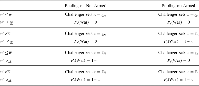
Table 1 summarizes the equilibria as a function of the Target’s decision to arm and the Challenger’s prior belief that the Target is weak. Note there are conditions under which the probability of war is unaffected by the Target’s decision. Specifically, when $w\prime\leq \bar{w}$ and $$w\prime\prime\leq \underline {w}$$ or when $w\prime\gt \bar{w}$ and $w\prime\prime\gt \underline {w}$ , the Target’s decision has no impact on the probability of war. In the former case, war never occurs; in the latter case, the Challenger risks war regardless of the Target’s decision.

Table 1

Summary of Equilibria

Note: w′ is the Challenger’s posterior belief the Target is weak given the Target is armed and w″ is the Challenger’s posterior belief the Target is weak given the Target did not arm. Cell entries report the demand the Challenger makes in equilibrium when the Target either pools on not arming (second column) or pools on arming (third column).

In contrast, when $w\prime\!\,\leq \,\bar{w}$ and $w\prime\prime\,\gt\, \underline {w}$ , the Challenger risks war if and only if the Target did not arm. In such cases, we would conclude that arming strictly prevents war. However, when $w\prime\,\gt\, \bar{w}$ and $w\prime\prime\,\leq\, \underline {w}$ , the Challenger risks war if and only if the Target does not arm. In such cases, arming promotes war.

However, unless we make some unusual assumptions about the beliefs held by the Challenger with respect to events that never occur in equilibrium, we can nonetheless conclude that arming more often than not prevents war. For example, suppose the Challenger’s off-the-equilibrium path belief matches the Challenger’s prior belief. As $\underline {w}\,\lt \,\bar{w}$ , it is impossible for $w\prime\gt \bar{w}$ and $w\prime\prime\!\,\leq\, \underline {w}$ to simultaneously hold. If we relax this assumption and allow off-the-equilibrium path beliefs to take on any value, we need only assume they are distributed similarly to the Challenger’s prior beliefs in order to conclude the conditions under which arming strictly reduces the probability of war will be met more often than the conditions under which arming promotes war. As we discuss below, this is precisely what we assume in our simulated data.

If and only if both types of Target arm, and the Challenger’s prior belief the Target is weak is sufficiently large, then the Challenger is willing to risk war with a relatively large demand, but the Challenger would believe the Target is less likely to be weak if the Target did not arm, then we would conclude that arming promotes war. It is unclear why the Challenger would be expected to hold such a belief as the stronger Target does not face a greater incentive to deviate from the equilibrium strategy of arming.

Nonetheless, in our simulated data, we allow the Challenger’s out-of-equilibrium belief to take on any value with equal probability, and still conclude arming reduces the probability of war. Therefore, there are some observations for which the equilibrium probability of war is non-zero, but had the Target deviated from the equilibrium strategy and chosen not to arm, the probability of war would be zero. For this reason, we stress the true relationship between arming and war in our simulated data is that, on average, arming reduces the probability of war. There are more cases where this is true than where it is not.

Scholars who are not persuaded by our treatment of out-of-equilibrium beliefs should note, irrespective of whether such assumptions would be warranted if our goal was to use the model to generate observable implications that were then tested with observational data, given the way we set up our Monte Carlo simulations, we must nonetheless conclude we are being misled by statistical models that fail to identify that, within our simulated data, arming generally reduces the probability of war.

IMPLICATIONS

The equilibria discussed above have several important properties useful for our Monte Carlo simulations, where we treat the model as the complete DGP. We do so not because we believe this to be plausible, but rather because it illustrates the problem more clearly.Footnote ⁸

First, the model generates equilibria in which war occurs despite the Target choosing to arm. As we evaluate a probabilistic relationship between arming and conflict, the absence of such equilibria could introduce the zero-likelihood problem. Second, the use of matching is more straightforward when the treatment is binary. Treating the decision to arm as binary in the formal model allows us to use a binary treatment without compromising the connection between the model and the simulated data. Finally, although there are eight different equilibria, each one occupies a unique subset of the parameter space. Thus, we do not need to make arbitrary decisions about equilibrium selection. For any given set of parameter values, we can uniquely identify each player’s strategies and the resulting probability of war.

It is useful to express the implications of the model more precisely using the potential outcomes framework. Let Y _i1 be a binary indicator for whether observation i experiences conflict given the Target armed (is treated) and Y _i0 be a binary indicator for whether i experiences conflict given the Target did not arm (is untreated). The fundamental problem of causal inference is that for each i, only one of these outcomes is observed. If a state arms, we cannot know what would have happened if the state did not arm. Similarly, if a state does not arm, we cannot observe what would have happened had it armed. As we cannot observe counterfactual states of the world, two of the four quantities of interest are unobservable, and we cannot directly assess the causal effect of the treatment on any given observation.

What we can do is compare the outcomes of those states that did not arm to the outcomes of those that did and hope that any differences we observe are owing to the fact one set of states armed and one did not. However, this only facilitates correct inferences if we correct for all other relevant differences between those states that armed and those that did not. This is no small caveat, given we have theoretical reason to believe we cannot hope to perfectly distinguish empirically between states engaged in crisis bargaining and those that are not, nor between instances where states unilaterally alter the status quo to minimize the risk of war versus those where states believed they pushed their opponent to the brink, yet were fortunate to discover the other side was willing to allow their fait accompli to stand.

We focus on the average treatment effect for the treated (ATT), rather than the average treatment effect for the control (ATC). The ATT $(\tau _{t} )$ is τ|(T=1)=E(Y _i1|T _i =1)−E(Y _i0|T _i =1) and ATC (τ _c ) is τ|(T=0)=E(Y _i1|T _i =0)−E(Y _i0|T _i =0), where T _i =1 indicates that i is in the treatment regime (armed) and T _i =0 that i is in the control regime (did not arm). That is, we focus on whether observations where the Target armed would have experienced a lower probability of conflict if the Target did not arm. This is related to, but distinct from, the question of whether the probability of war among those observations where the Target did not arm would have been higher had the Target armed. We focus on the former because, although the effects are substantively similar in both cases, the ATT should be larger and the failure to properly identify it would be more striking than the failure to properly identify the ATC.Footnote ⁹

Yet, as mentioned above, there may be reasons to suspect that it is difficult to determine which states are engaged in crisis bargaining. As crisis bargaining is a predictor of both war and arming, we have reason to doubt that extant empirical analysis has identified the true relationship between arming and war.

We are not claiming to know that arming prevents war. It is entirely possible that the theoretical models that suggest it does are over-simplified. Our argument is simply that even if it were true that arming prevents war, we might falsely conclude that it does not—and this is a much harder problem to solve than is commonly appreciated, even when using techniques designed to solve such problems.

Table 1 shows that when $w\prime\leq \bar{w}$ and $w\prime\prime\!\,\leq \,\underline {w}$ or when $ w\prime\gt \,\bar{w}$ and $w\prime\prime\gt \underline {w}$ , the probability of war does not depend on the Target’s decision to arm. In the language of potential outcomes, that means there are cases for which $\tau _{t} =E(Y_{{i1}} ){\minus}E(Y_{{i0}} )=0$ . The same will be true for all observations where the states did not engage in crisis bargaining, as the probability of war in these cases is 0 by assumption, regardless of treatment status.

There also exist cases where E(Y _i1)−E(Y _i0)>0 as well as cases where E(Y _i1)−E(Y _i0)<0.Footnote ¹⁰ That is, it is possible that arming can either prevent or promote war. However, the conditions under which there is a positive probability of war if and only if the Target arms are restrictive. Given the distribution of beliefs for the Challenger that we use in our Monte Carlo simulations (see web appendix), we can be confident the τ _t and τ _c will be negative, and thus, if we fail to identify a negative τ _t and τ _c within our simulated data we will draw an incorrect inference regarding the effect of arming on the likelihood of war.

SIMULATED DATA

We generate the military capabilities for State 1 and State 2 for 100,000 dyads.Footnote ¹¹ Specifically, CAP ₁~N(0.5,0.05), CAP ₂ ^L ~N(0.5,0.05), and CAP ₂ ^H =CAP ₂ ^L +ϵ, where ϵ~N(1,0.1). In the bargaining model, CAP ₁ represents m ₁, CAP ₂ ^L represents $\underline {m}_{2} $ , and CAP ₂ ^H represents $\bar{m}_{2} $ . Next, we generate ALPHA~N(0.5,0.05) for α, KAPPA~N(0.5,0.005) for k, and COST _i ~N(0.1,0.01) for i∈{1,2} for c _i .Footnote ¹²

BARG is a binary variable indicating whether the states in the dyad engaged in crisis bargaining, which is true for ≈10 percent of the observations (randomly selected). We assume crisis bargaining is perfectly described by the model.Footnote ¹³ Ultimately, WAR=1 in 20 percent of the observations where BARG=1. Given we assume the path to war is perfectly captured by our theoretical model, when BARG=0, war is never observed.

If State 2 arms in order to deter one potential aggressor, their arming decision will be reflected in all dyads containing State 2, as we cannot readily determine which state prompted an increase in State 2’s military capabilities. We create a binary variable ARM, which equals 1 when BARG=1 and the formal model indicates State 2 would arm, and equals 1 when BARG=0 with probability 0.25 if $KAPPA\leq \overline{{KAPPA}} $ , and with probability 0.1 if $KAPPA\gt \overline{{KAPPA}} $ . Overall, ARM=1 in 41 percent of the observations when BARG=1 and 18 percent when BARG=0.

IV ₁ and IV ₂ are instruments for ARM. IV ₁=1 with probability 0.75 if KAPPA≤0.05 and 0 otherwise. IV ₂ is constructed identically, except the probability is 0.9. IV ₁=1 ≈34 percent of the time when ARM=0, and 53 percent of the time when ARM=1. For IV ₂, these figures are 40 and 64 percent, respectively.

As interstate wars are relatively rare, scholars often test hypotheses about war using lower levels of hostility, such as Militarized Interstate Disputes (MIDs). We create a variable MID that equals 1 when WAR=1 but also equals 1 with probability 0.75 if BARG=1 and WAR=0, and with probability 0.05 when BARG=0. Approximately 64 percent of our simulated MIDs reflect actual crises, in that the states played the crisis bargaining game.

A few characteristics of MID are worth emphasizing. First, a greater percentage of our simulated MIDs represent wars than is typically true when using the actual MID data. WAR=1 in 16 percent of our observations when MID=1. In contrast, <4 percent of the MIDs in the data used by Bennett and Stam (Reference Bennett and Stam2004) are wars, for example. Our results will therefore underestimate the problems with testing hypotheses about war using a dependent variable that measures lower levels of hostility, as our simulated MID variable is less distinct from WAR than is the case of actual MIDs.

Second, BARG=0 for a substantial number of observations where our simulated MID variable equals 1 (≈36 percent). The MID data were designed to minimize the possibility of such cases. “States do not engage in militarized actions unless they perceive that the issues at stake are important, and… we believe that militarization is a valid indicator that a dispute is serious” (Jones, Bremer and Singer Reference Jones, Bremer and Singer1996, 168). Thus, our MID variable may correlate with BARG to a lesser extent than is the case in the actual data. It is important to note this also ensures we are underestimating the problems associated with testing hypotheses about the causes of war using the MID data. As MID and BARG become less distinct, we become more likely to estimate a positive relationship between ARM and MID, given that BARG predicts ARM.

We also create a variable to indicate whether State 2 reciprocated State 1’s hostility, as per the same variable in the MID data. Specifically, we set RECIP=1 with certainty if WAR=1, with probability 0.5 if BARG=1, MID=1, and WAR=0, and with probability 0.075 if BARG=0, MID=1, and WAR=0. RECIP is coded as missing if MID=0. Approximately 43 percent of our simulated MIDs involve reciprocated hostility.

Although we assume BARG is unobservable, we generate two binary variables, PROX ₁ and PROX ₂, which we assume are observable and can be used to indicate which dyads are likely to experience conflict. These variables might represent geographic contiguity or rivalry, which have been shown to influence conflict onset. Importantly, neither contiguity nor rivalry need to be considered a cause of conflict so much as a strong indicator of which states are likely to engage in crisis bargaining.

We set PROX ₁=1 with probability 0.5 if BARG=1, and probability 0.1 if BARG=0, whereas PROX ₂=1 with probability 0.3 if BARG=1, and probability 0.1 if BARG=0. We refer to the data set containing these variables as Experiment 1.

Next, we generate a simulated data set identical to the first one, except PROX ₁=1 with probability 0.4 if BARG=1, and probability 0.15 if BARG=0, whereas PROX ₂=1 with probability 0.2 if BARG=1, and probability 0.1 if BARG=0. We refer to this data set as Experiment 2.

BASELINE ANALYSIS

We illustrate the problem by comparing the results from a naïve research design to those obtained after conditioning on the unobservable variable BARG, which is not possible in practice.Footnote ¹⁴ For our naïve research design, we estimate binary logits using MID and WAR as dependent variables. The primary independent variable is ARM, although we include the proxy variables from Experiments 1 and 2. We initially include all dyads, as is common in applied research. Next, we match on BARG. For these models, we do not include our proxy variables as they are no longer necessary to isolate the systematic difference between the treatment and control groups.

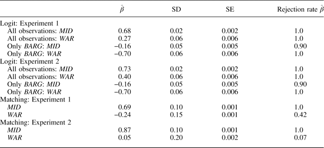
Table 2 summarizes the results from 100 independently created data sets, each of which was constructed as described above. We report the mean and standard deviation of the coefficient estimate for ARM $$(\hat{\beta })$$ across the 100 estimated models.Footnote ¹⁵ We also report the standard error $$\left( {{s \over {\sqrt {100} }}} \right)$$ and the rejection rate of $\hat{\beta }$ based on H _o: β=0 versus H _a : β≠0 using a two-tailed test and significance level of p<0.05.Footnote ¹⁶

Table 2

Summary of Results (Logit, Matching)

Note: results based on 100 independent data sets. Results only reported for ARM. For matching models, results reported after matching on PROX ₁=PROX ₂=1.

The top panel of Table 2 contains the results. When the analysis includes all dyads, we always estimate a positive relationship between arming and conflict, irrespective of whether conflict is measured using MID or WAR, for both Experiments 1 and 2. We also always reject the null hypothesis when analyzing all dyads.

In contrast, when we condition on BARG, we always observe the negative relationship anticipated by the formal model, regardless of the dependent variable and for both Experiments 1 and 2.Footnote ¹⁷ In addition, we always reject the null hypothesis when we condition on BARG and WAR is the dependent variable, and nearly always when MID is the dependent variable. This clearly illustrates the problem is our inability to determine who is engaged in crisis bargaining.

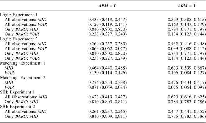
Note while the choice of dependent variable (MID versus WAR) does not change the interpretation of the overall relationship between ARM and conflict, it does affect the size of the effect. Table 3 shows the predicted probabilities and 95 percent confidence intervals when PROX ₁=PROX ₂=1, which corresponds to the case where states are most likely to arm, from which we can estimate $\hat{\tau }_{t} $ .Footnote ¹⁸ When we include all dyads, the change in the size of the effect is larger for MID compared with WAR. However, the change in the size of the effect when we condition on BARG is larger for WAR compared with MID. ARM decreases the probability of WAR by 0.10 among those dyads engaged in crisis bargaining. However, among the same dyads, ARM only decreases the probability of MID by 0.03.

Table 3

Predicted Probabilities (Logit, Matching, and SBI Models)

Note: results based on 100 independent data sets. For matching models, results reported after matching on PROX ₁=PROX ₂=1. Statistical backwards induction (SBI) models that only include observations where BARG=1 exclude PROX ₁ and PROX ₂ and are based on CAP ₁ held at mean value of 0.5.

Despite including control variables (PROX ₁ and PROX ₂) we always estimate a positive $\hat{\tau }_{t} $ when analyzing all dyads. Once we condition on BARG we correctly identify a negative $\hat{\tau }_{t} $ using a binary logit. The problem is we cannot condition on this variable in practice.

MATCHING

We now discuss the results after matching on PROX ₁=PROX ₂=1.Footnote ¹⁹ We implicitly employed exact matching (using BARG), and correctly identified a negative $\hat{\tau }_{t} $ .Footnote ²⁰ However, matching does not reliably uncover treatment effects when confounders are unobservable, as this violates the assumption of conditional independence (Sekhon Reference Sekhon2008).Footnote ²¹ We know we have violated this assumption. In practice, researchers cannot know whether they have done so. All they can do is demonstrate their matched data set is balanced with respect to observable covariates and hope for the best.

We focus on exact matching, which is the preferred approach when feasible.Footnote ²² Exact matching isolates much, but not all, of the difference between treatment and control groups. In our simulated data, BARG is 2.8 times as likely to equal 1 when ARM=1 before matching, versus 1.46 after matching in Experiment 1 and 1.94 in Experiment 2.Footnote ²³

The bottom panel of Table 2 summarizes the results.Footnote ²⁴ In the baseline analysis, the primary difference between the models where the dependent variable was MID and those where it was WAR was the magnitude of the effect of ARM. Here, in both Experiments 1 and 2, we estimate a positive relationship between ARM and MID and always reject the null hypothesis. When WAR is the dependent variable we identify a positive $\hat{\tau }_{t} $ in Experiment 2 but a negative $\hat{\tau }_{t} $ in Experiment 1; however, we do not always reject the null hypothesis in either experiment. Thus, if we select a more appropriate dependent variable, we might at least avoid drawing the opposite conclusion, though we would fail to uncover the pacifying effect of arming.

The middle panel of Table 3 shows the predicted probabilities and 95 percent confidence intervals when ARM=0 and ARM=1. ARM increases the probability of MID by 0.17 and 0.20 in Experiments 1 and 2, respectively, and increases the probability of WAR by 0.004 in Experiment 2, but decreases the probability of WAR by 0.02 in Experiment 1. In the baseline analysis ARM decreased the probability of WAR by 0.10, five times larger than the effect observed here. Thus, we underestimate the magnitude of the relationship between ARM and WAR even when the direction of the effect is correct.

These results highlight a common misconception about the inclusion of control variables in generalized linear models. Such practice does not justify the use of “all else equal” language, so common in applied research. Our proxy variables are capable, under some conditions, of leading us to the correct inference when we used them for matching, but did not do so when included as controls in the baseline analysis.

Note, we have addressed neither the Stable Unit Treatment Value Assumption (SUTVA), nor whether our conditioning variables were determined before treatment status; here neither is a concern; however, in practice, they very well might be.Footnote ²⁵ Thus, we stress that whereas matching sometimes enabled us to correctly identify a negative $\hat{\tau }_{t} $ , it did not always, and many of the assumptions we made would be untenable in practice.

INSTRUMENTAL VARIABLES

Unlike matching methods, instrumental variables can enable researchers to uncover the true causal effect even when there are unobserved confounders.Footnote ²⁶ By construction, our instruments (IV ₁ and IV ₂) are correlated with ARM but are not directly related to either of our dependent variables (MID and WAR). Moreover, we can be sure the average effect of ARM is non-zero and monotonic. Therefore, we have satisfied the assumptions required for drawing causal inferences using instrumental variables (Angrist and Pischke Reference Angrist and Pischke2009).Footnote ²⁷

For Experiments 1 and 2, we estimate four bivariate probit models.Footnote ²⁸ We model ARM as a function of the binary instrument and the proxy variables, and conflict as a function of ARM and the proxy variables. The log-likelihood function for each model is

(1) $$\eqalignno{ \mathop{\sum} &#x0026; \left[ {Y_{i} \;{\rm ln}\;\Phi _{b} \left( {{{X_{i} \beta _{0} {\plus}ARM_{i} \beta _{1} } \over {\sigma _{{\varepsilon}} }},{{X_{i} \gamma _{0} {\plus}IV_{i} \gamma _{1} } \over {\sigma _{\nu } }};\rho _{{{\varepsilon}\nu }} } \right)} \right. \cr &#x0026; {\plus}\left. {(1{\minus}Y_{i} )\;{\rm ln}\;\left[ {1{\minus}\Phi _{b} \left( {{{X_{i} \beta _{0} {\plus}ARM_{i} \beta _{1} } \over {\sigma _{{\varepsilon}} }},{{X_{i} \gamma _{0} {\plus}IV_{i} \gamma _{1} } \over {\sigma _{\nu } }};\rho _{{{\varepsilon}\nu }} } \right)} \right]} \right], $$

where Y _i is either MID or WAR, X _i =PROX ₁+PROX ₂, β ₀ and β ₁ are coefficients to be estimated in the second stage, γ ₀ and γ ₁ are coefficients to be estimated in the first stage, ϵ the error term for the second stage, v the error term for the first stage, and $$\Phi _{b} ( \cdot , \cdot ,\rho _{{{\varepsilon}\nu }} )$$ the bivariate normal cumulative distribution function with correlation coefficient ρ _ϵv .

We are primarily interested in $$\hat{\tau }_{t} =E[Y_{{1i}} {\minus}Y_{{0i}} \,\mid\,IV_{i} =1]$$ . As Angrist and Pischke (Reference Angrist and Pischke2009, 200–1) discuss:

(2) $$\hat{\tau }_{t} =E\left[ {{{\Phi _{b} \left( {{{X_{i} \hat{\beta }_{0} {\plus}\hat{\beta }_{1} } \over {\sigma _{{\varepsilon}} }},{{X_{i} \hat{\gamma }_{0} {\plus}IV_{i} \hat{\gamma }_{1} } \over {\sigma _{\nu } }};\rho _{{{\varepsilon}\nu }} } \right)\,{\minus}\,\Phi _{b} \left( {{{X_{i} \hat{\beta }_{0} } \over {\sigma _{{\varepsilon}} }},{{X_{i} \hat{\gamma }_{0} {\plus}IV_{i} \hat{\gamma }_{1} } \over {\sigma _{\nu } }};\rho _{{{\varepsilon}\nu }} } \right)} \over {\Phi_b \left( {{{X_{i} \hat{\gamma }_{0} {\plus}IV_{i} \hat{\gamma }_{1} } \over {\sigma _{\nu } }}} \right)}}} \right].$$

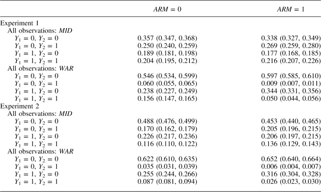
Equation 2 defines $$\hat{\tau }_{t} $$ as the difference in the expected probability of conflict given the Target armed and the expected probability of conflict given the Target did not arm divided by the expected probability the Target arms. Thus, $$\hat{\tau }_{t} $$ can be identified readily from the predicted probabilities, which are presented in Table 4. We calculate $$\hat{\tau }_{t} $$ when IV ₁=PROX ₁=PROX ₂=1, thereby maximizing the probability of treatment.Footnote ²⁹

Table 4

Predicted Probabilities (Instrumental Variables)

Note: results based on 100 independent data sets. Results based on IV ₁=1 and PROX ₁=PROX ₂=1.

For Experiment 1, when Y _i is given by MID, we calculate $$\hat{\tau }_{t} \approx{\minus}0.08$$ .Footnote ³⁰ We calculate $$\hat{\tau }_{t} \approx{\minus}0.03$$ for WAR. For Experiment 2, $$\hat{\tau }_{t} $$ is −0.10 and −0.03, respectively. Thus, $$\hat{\tau }_{t} $$ is consistently negative, although surprisingly, the estimated effect is larger for MID than WAR.Footnote ³¹

These results are only somewhat encouraging. We implicitly made some strong assumptions and we did not discuss local treatment effects nor how we might identify an instrument for arming.Footnote ³² These concerns are difficult to ignore when analyzing real data.Footnote ³³

SBI

Finally, we assess the prospects for identifying the negative relationship between arming and conflict using structural estimation, specifically SBI. SBI has the advantage of being simpler to employ than most structural estimators derived explicitly from game-theoretic models, with a minimal loss of efficiency (see Signorino Reference Signorino1999; Signorino Reference Signorino and Yilmaz2003; Signorino and Yilmaz Reference Slantchev2003).

We assume a similar game structure to that presented in Bas, Signorino and Walker (Reference Bas, Signorino and Walker2008). Specifically, we implement SBI assuming the game begins with a decision by the Challenger to accept the status quo or initiate a crisis, in which case the Target decides to concede or reciprocate, where reciprocation produces a conflict.

There are two important differences between this extensive form and the one in our crisis bargaining model. First, when using SBI, the good in dispute is treated as indivisible.Footnote ³⁴ It is difficult to determine the importance of this difference. For example, it is possible in practice the decision to initiate a MID approximates the decision to propose a division of the good in dispute that runs a greater risk of rejection. Unfortunately, few scholars have addressed the question of what MIDs actually represent with respect to bargaining outcomes.

Second, we do not treat the decision to arm as endogenous in the model that will be tested using SBI. Rather, our application of SBI treats this decision as given and seeks to evaluate its influence on the player’s subsequent decisions by assuming each player’s payoff for conflict depends on whether the Target armed previously. This is very likely an important difference. We stress we do not intend the analysis to serve as a test of the power of properly applied and theoretically appropriate structural estimators. A growing literature on this topic strongly indicates that such applications are powerful and we hope to see their use become more common. Our goal is to demonstrate the pitfalls associated with conducting empirical analysis divorced from prevailing theories and that this problem may not be solved by more sophisticated methods. In short, we believe many scholars might assume this game structure because of the ease with which it can be implemented, thanks to the sample code provided by Bas, Signorino and Walker (Reference Bas, Signorino and Walker2008).

Naturally, it would be more appropriate to analyze escalation to war within the subset of observations we can be confident are engaged in crisis bargaining, even if we continued to treat the decision to arm as exogenous. In fact, we demonstrate that if it were possible to observe BARG, one could uncover the correct inference even using the game structure that underlies our application of SBI.Footnote ³⁵

We specify the utilities at each terminal node as follows.Footnote ³⁶ As Bas, Signorino and Walker (Reference Bas, Signorino and Walker2008) point out, it is necessary to constrain one of the utilities to 0 in order to identify the model. Following their suggestion, we assign a value of 0 to the Challenger’s utility for the status quo, and the Target’s utility for conceding. The remaining utilities (the payoffs for each player in the event the Target reciprocates, and the Challenger’s utility for the Target conceding) consist of three parts: a coefficient, a set of regressors, and an error term. Formally, let X _cC β _cC represent the Challenger’s utility for having the Target concede, X _cR β _cR the Challenger’s utility for the Target reciprocating, and X _tR β _tR the Target’s utility for reciprocating. For simplicity, let X _cC =1, X _cR0=1, X _cR1=(1−ARM), X _cR2=CAP ₁, X _tR0=1, X _tR1=ARM, X _tR2=PROX ₁, and X _tR3=PROX ₂.Footnote ³⁷

We require the player’s choices to be probabilistic. Therefore, we assume the Target reciprocates if X _tR β _tR +ϵ _t >0 and the Challenger initiates an MID if (1−p_r )(X _cC β _cC )+(p_r )(X _cR β _cR +ϵ _c )>0, where p_r is the probability the Target reciprocates. Here, ϵ _c and ϵ _t can be interpreted as either agent error or private information. As long as we assume that we as analysts cannot know the true value of ϵ _c and ϵ _t , whereas the Challenger knows the value of ϵ _c but not ϵ _t and the Target knows the value of ϵ _t but not ϵ _c , we can remain agnostic as to whether these terms reflect agent error, and thus sub-optimal or non-Nash play, or private information held by actors who behave optimally given their information.Footnote ³⁸ We also assume ϵ _c and ϵ _t are independently distributed Type I Extreme Value, such that the choice probabilities are logit probabilities with uncorrelated error terms (Bas, Signorino and Walker Reference Bas, Signorino and Walker2008, 27).

The effect of ARM is ambiguous. By construction, ARM has two important effects. Most obviously, setting X _cR1=(1−ARM) ensures the Challenger’s utility for reciprocation is decreasing in ARM. However, ARM is also in X _tR . Provided β _tR1>0, this effect increases p_r . Whether an increase in p_r increases or decreases the probability that MID=1 is unclear, as X _cC β _cC may be either larger or smaller than X _cR β _cR .Footnote ³⁹

We estimate $\hat{p}_{c} $ and $\hat{p}_{r} $ as follows. We first estimate a logit with RECIP as the dependent variable. We evaluate the probability of reciprocation using X _tR . The predicted probabilities generated from this model produce $\hat{p}_{r} $ . Next, we construct $Z_{{cC}} =(1{\minus}\hat{p}_{r} )X_{{cC}} $ and $$Z_{{cR}} =\hat{p}_{r} X_{{cR}} $$ . We then estimate a second logit with MID as the dependent variable and Z _cC and Z _cR as the independent variables. This ensures the coefficient estimates for Z _cC and Z _cR will be $\hat{\beta }_{{cC}} $ and $\hat{\beta }_{{cR}} $ , providing estimates of the β terms identified above.Footnote ⁴⁰ As the regressors in the second logit are predicted probabilities, we calculate bootstrapped standard errors in order to avoid biased estimates for the standard errors of $\hat{\beta }_{{cC}} $ and $\hat{\beta }_{{cR}} $ .Footnote ⁴¹

The bottom panel of Table 3 shows the predicted probabilities of MID and 95 percent confidence intervals when PROX ₁=PROX ₂=1, which corresponds to the case where states are most likely to arm, for Experiments 1 and 2.Footnote ⁴² We held CAP ₁ at its mean value of 0.5.Footnote ⁴³ In Experiment 1, ARM increases the probability of a MID $(\hat{p}_{c} )$ by 0.20. In Experiment 2, ARM increases the probability of MID by 0.19. These results indicate that SBI, using a specification similar to that in Bas, Signorino and Walker (Reference Bas, Signorino and Walker2008), is unlikely to correctly identify the relationship between ARM and conflict. However, we wish to be clear about the source of the problem, which is not a fundamental flaw in the logic underlying SBI.

To illustrate this, we follow the same procedure as above, with two changes. First, we only focus on observations where BARG=1. Second, because we have little reason to expect PROX ₁ or PROX ₂ to capture important variation in this subset of observations, we drop X _tR2 and X _tR3 from X _tR . These results show that arming decreases the probability of a MID by 0.03 in both Experiments 1 and 2. This reinforces our claim that the problem is that BARG is unobservable rather than a fundamental shortcoming of SBI.

We also stress that we focus on the simplest possible application of SBI rather than one that is more theoretically appropriate (i.e., one where we treat ARM as endogenous, as in the bargaining model that we presented above). Our goal is to illustrate the consequences of failing to think seriously about the implications of prevailing theoretical arguments, as an uncritical adaptation of Bas, Signorino and Walker (Reference Bas, Signorino and Walker2008) does, rather than to assess the performance of structural estimators that are theoretically motivated, which we have every reason to believe would perform much better.

SUMMARY OF RESULTS

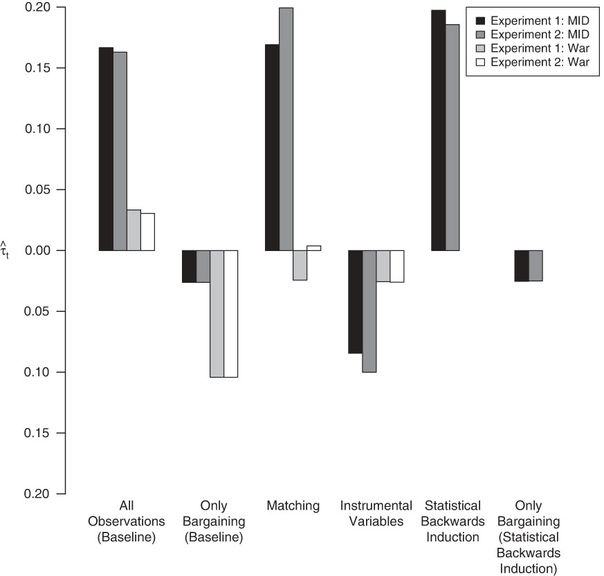
Throughout this article, we focussed on $$\hat{\tau }_{t} $$ , the ATT. Put differently, we focussed on the difference between the observed likelihood of conflict for those observations where the Target armed and the counterfactual likelihood of conflict that would have been observed for those observations had the Target not armed. Figure 1 presents the estimated $$\hat{\tau }_{t} $$ for our baseline analysis and each of the three statistical methods discussed above.

Fig. 1

Comparison of baseline models and three empirical methods

Overall, the results from the bivariate probit models with instrumental variables performed best, consistently estimating a negative $$\hat{\tau }_{t} $$ , regardless of the dependent variable or the quality of the proxy variables. Our simplistic approach to SBI fared worst of all. Matching on observables uncovered a negative effect for Experiment 1 when the dependent variable was WAR.

There are important lessons to be learned from these results. First, if BARG was observable, sophisticated methods would not be necessary to correctly infer that, on average, potential Targets are less likely to experience conflict if they arm. Second, the method that performed best was the only one that explicitly modeled the Target’s decision to arm. This suggests that scholars who hope to simply “let the data speak” without thinking carefully about how the data were generated are likely to draw incorrect inferences.

However, things may be different in practice. Instrumental variables may not outperform the other approaches if $$\hat{\tau }_{t} $$ and $$\hat{\tau }_{c} $$ work in different directions, for example, as this would violate the monotonicity assumption. In addition, structural estimators that are closely linked to strong theoretical arguments should perform better.