1. Introduction
The Richtmyer–Meshkov instability (RMI) is a hydrodynamic instability that occurs when a shock wave interacts with a perturbed interface separating two fluids of different densities (Richtmyer Reference Richtmyer1960; Meshkov Reference Meshkov1969; Zhou Reference Zhou2024). Initially proposed by Richtmyer (Reference Richtmyer1960) as a shock-accelerated counterpart to the Rayleigh–Taylor instability (RTI) (Rayleigh Reference Rayleigh1882; Taylor Reference Taylor1950), it was later confirmed experimentally by Meshkov (Reference Meshkov1969). When the incident shock is perturbed, the subsequent instability is referred to as the non-standard RMI (Zhou Reference Zhou2017; Zou et al. Reference Zou, Al-Marouf, Cheng, Samtaney, Ding and Luo2019). Unlike RTI, which arises under sustained acceleration, RMI is triggered by an impulsive acceleration from a shock wave, leading to the growth of initial perturbations at the interface. These perturbations evolve into complex structures, such as bubbles and spikes, eventually causing turbulent mixing between the fluids. Studying RMI holds critical importance across multiple disciplines. In astrophysics, it helps to explain shock-driven mixing processes in supernovae, where heavy and light elements intermingle during stellar explosions (Abarzhi et al. Reference Abarzhi, Bhowmick, Naveh, Pandian, Swisher, Stellingwerf and Arnett2019). For inertial confinement fusion (ICF), RMI-induced mixing can degrade fuel compression symmetry, reducing energy yield, which is a key challenge in achieving sustainable fusion ignition (Lindl et al. Reference Lindl, Landen, Edwards, Moses and team2014; Zhou et al. Reference Zhou, Clark, Clark, Glendinning, Skinner, Huntington, Hurricane, Dimits and Remington2019, Reference Zhou, Sadler and Hurricane2025). In ICF plasmas, Tapinou et al. (Reference Tapinou, Wheatley, Bond and Jahn2022) have predicted and simulated the amplification of the original seed perturbation and the seeding of higher-wavenumber instabilities in ICF-type RMI, as well as the triggering of secondary instabilities. In aerospace engineering, understanding RMI aids in optimising scramjet combustors, where RMI will enlarge the reactive surface and dictate combustion efficiency (Napieralski et al. Reference Napieralski, Cobos, Sánchez-Sanz and Huete2024). Insights into RMI not only deepen knowledge of nonlinear fluid behaviour, enhancing our ability to control flow instabilities, but also drive innovations in energy technology (Zhou et al. Reference Zhou, Sadler and Hurricane2025) and space exploration (Khokhlov et al. Reference Khokhlov, Oran, Chtchelkanova and Wheeler1999).
In classical RMI studies, the focus is on a flat shock interacting with a perturbed interface, and significant achievements have been made in this domain (Yang et al. Reference Yang, Zhang and Sharp1994; Wouchuk Reference Wouchuk2001; Niederhaus & Jacobs Reference Niederhaus and Jacobs2003; Lombardini et al. Reference Lombardini, Hill, Pullin and Meiron2011; Zhang & Guo Reference Zhang and Guo2016; Zhai et al. Reference Zhai, Zou, Wu and Luo2018, Reference Zhai, Xu and Luo2024; Groom & Thornber Reference Groom and Thornber2023; Fu et al. Reference Fu, Wang, Lin, Zhu, Wang and Luo2025; Zhou et al. Reference Zhou, Sadler and Hurricane2025). Beyond classical RMI, the non-standard RMI induced by the interaction of a rippled shock wave with a material interface is also a fundamental phenomenon in compressible fluid dynamics (Zhou Reference Zhou2017; Zou et al. Reference Zou, Al-Marouf, Cheng, Samtaney, Ding and Luo2019). Here, the shock wave itself would carry perturbations due to upstream turbulence, surface roughness, or engineered disturbances, adding complexity to the interaction dynamics. In ICF, for example, non-uniform laser illumination induces localised pressure fluctuations at the ablation surface. These fluctuations imprint spatially correlated modulations onto the propagating shock front (Hu et al. Reference Hu, Michel, Davis, Betti, Radha, Campbell, Froula and Stoeckl2016), which subsequently seed hydrodynamic instabilities during the implosion phase (Campbell et al. Reference Campbell2021). As a result, understanding the non-standard RMI development is also a fundamental requirement for ICF.
Understanding non-standard RMI necessitates fundamental insights into the evolution of isolated rippled shock waves. A rippled shock propagating in an ideal gas is always asymptotically stable, with the perturbation amplitude on the shock front exhibiting oscillatory decay (Andrés et al. Reference Andrés, Alexander and César2023), regardless of the change in the gas specific ratio and the shock strength. The temporal evolution can be partitioned into distinct phases characterised by the sign of shock amplitude and its growth rate (Kane et al. Reference Kane2001; Zhang et al. Reference Zhang, Wu, Zou, Zheng, Li, Luo and Ding2018). In the first phase, the shock amplitude is positive and decays with time. The amplitude evolution of a rippled shock driven by a sinusoidal piston is called the Freeman problem (Freeman Reference Freeman1955). By introducing the hyperbolic-polar coordinate and applying the Laplace transform, Zaidel’ (Reference Zaidel’1960) revealed perturbation decay scaling as
 $t^{-3/2}$
(general case) or
 $t^{-1/2}$
(strong-shock limit) in an ideal gas. Subsequent studies confirmed the universality of this scaling (Nikolaev Reference Nikolaev1965; Briscoe & Kovitz Reference Briscoe and Kovitz1968). Bates (Reference Bates2004) derived an explicit solution that does not include infinite series for the evolution of the perturbation amplitude on an isolated two-dimensional rippled shock propagating in an inviscid fluid with an arbitrary equation of state. Recent advances by Wouchuk (Reference Wouchuk2025) provided explicit analytical solutions with a more compact form for late-time perturbations in corrugated shock/piston systems. These different theories mentioned above provide similar predictions to shock front perturbations.
The study of non-standard RMI builds upon seminal theoretical frameworks established by Ishizaki et al. (Reference Ishizaki, Nishihara, Sakagami and Ueshima1996), referred to as the IN model hereafter. This model associates the interface perturbation growth rate and the shock perturbation growth rate with an empirical parameter
 $D= 0.66$
calibrated for a Mach 2.0 shock. Kane et al. (Reference Kane2001) performed laser-driven shock imprint experiments, validating the phase-dependent effects of shock perturbations on interface evolution. Subsequently, non-standard RMI was investigated, respectively, in planar (Zou et al. Reference Zou, Liu, Liao, Zheng, Zhai and Luo2017) and cylindrical (Liang et al. Reference Liang, Ding, Zhai, Si and Luo2017; Zou et al. Reference Zou, Al-Marouf, Cheng, Samtaney, Ding and Luo2019) geometries, in which the rippled shock was generated by diffraction of a planar shock over the rigid cylinders. In the classical RMI, the growth rate of perturbation amplitude is proportional to Atwood number. By contrast, Zou et al. (Reference Zou, Al-Marouf, Cheng, Samtaney, Ding and Luo2019) found that the growth rate of perturbation amplitude has a weak dependence on Atwood number in the deformed shock-induced RMI. However, the rippled shock fronts are non-sinusoidal, and are characterised by Mach stems and triple points. Therefore, the shock amplitude evolution deviates from Bates theory (Liang et al. Reference Liang, Ding, Zhai, Si and Luo2017). These studies attempted to establish a geometric equivalence between classical and non-standard RMI, but revealed fundamental dissimilarities in perturbation evolution mechanisms between them (Zou et al. Reference Zou, Liu, Liao, Zheng, Zhai and Luo2017). Through shock refraction at a gas interface to produce the rippled shock wave, Zhang et al. (Reference Zhang, Wu, Zou, Zheng, Li, Luo and Ding2018) numerically investigated Mach number effects on non-standard RMI. Their findings demonstrated the sensitivity of empirical coefficients in the IN model to both shock phase and intensity. Within the vorticity dynamics framework (Samtaney et al. Reference Samtaney, Ray and Zabusky1998), the baroclinic vorticity deposition was modelled and the non-standard RMI evolution was studied in both planar and convergent geometries (Li et al. Reference Li, Ding, Luo and Zou2022; Zhang et al. Reference Zhang, Zhao, Ding and Luo2023). The solutions, however, cannot give an explicit growth rate prediction, but rather need numerical integrals. Recently, Zhang et al. (Reference Zhang, Liao, Zou, Zhai, Liu and Li2024) investigated the development of planar interfaces accelerated by a rippled shock featured with triple-shock configurations through shock polar analysis. Their analyses revealed that velocity perturbations supersede vorticity in dominating the light–heavy interface evolution.
To sum up, compared to classical RMI, non-standard RMI has received far less attention, with the mechanisms driving its evolution remaining poorly understood, and the development of relevant theoretical models being notably scarce. Currently, only the IN model is available for non-standard RMI, but it relies on empirical coefficients. In addition, the IN model is applicable only to non-standard RMI when a rippled shock interacts with a uniform interface (Ishizaki et al. Reference Ishizaki, Nishihara, Sakagami and Ueshima1996; Zhang et al. Reference Zhang, Wu, Zou, Zheng, Li, Luo and Ding2018), and no models are available if perturbations are initially present at both shock wave and interface. Therefore, it is imperative to establish theoretical models for non-standard RMI. Moreover, although the previous work has identified the dissimilarity between the classical and non-standard RMI, the specific physical origins of these disparities have yet to be fully elucidated. These motivate the present work.
In the present study, an analytical model is first proposed to predict the amplitude evolution of a flat or rippled heavy–light interface subjected to a rippled shock wave, then numerical validations are performed. Based on the analytical model, the disparities between the classical and non-standard RMI are elucidated. Finally, the amplitude attenuation of the interface perturbation is examined to further validate the analytical model.
2. Theoretical derivation
2.1. Irrotational model establishment
A schematic of non-standard RMI is presented in figure 1. Assuming that an initially perturbed interface with the profile
 $x=a^0\cos {(ky)}$
in the flow field separates fluid
a
and fluid
b
, where
 $a^0$
is the initial perturbation amplitude, and
 $k$
is the perturbation wavenumber. The initial density and adiabatic ratio of the two fluids are
 $\rho _{{m0}}$
and
 $\gamma _{{m}}$
, respectively, with the subscript m
 $\,=\,$
a
,
b
referring to different fluids, and
 $\rho _{\boldsymbol{a}{0}}\lt\rho _{\boldsymbol{b}{0}}$
in this work. A rippled incident shock (IS) with initial amplitude
 $a^0_{{s}}$
propagates downstream along the
 $x$
-direction in fluid
b
, as shown in figure 1(a). The mean pressures ahead of and behind the incident shock are
 $p_0$
and
 $p_1$
, respectively. At
 $t=0$
, the IS interacts with the interface, generating a downstream transmitted shock (TS) and an upstream reflected rarefaction wave (RW), as shown in figure 1(b). The unperturbed background velocities for IS and TS are
 $V_{{I}}$
and
 $V_{{T}}$
, respectively. The balanced position of the shocked interface (SI) moves with velocity
 $\Delta \!V$
. The velocities are evaluated under a laboratory coordinate. Zones
af and
bf are the shocked fluid bulks near the interface in fluids
a
and
b
, respectively. The balanced pressure near the interface is
 $p_{{\! f}}$
. The parameters in zones
af and
bf can be derived through one-dimensional gas dynamics, as provided in Appendix A.
Schematic of non-standard RMI: (a) before shock–interface interaction; (b) after shock–interface interaction. Here, IS means rippled incident shock, II means initial interface, RW means reflected rarefaction wave, SI means shocked interface, TS means transmitted shock;
 $\rho _{{\boldsymbol{a}0}}$
and
 $\rho _{{\boldsymbol{b}0}}$
are initial densities of fluids
 $\boldsymbol{a}$
and
 $\boldsymbol{b}$
;
 $\rho _{{\boldsymbol{b}1}}$
is the density of fluid
 $\boldsymbol{b}$
behind IS;
 $\rho _{\boldsymbol{a}{\!f}}$
and
 $\rho _{\boldsymbol{b}{\!f}}$
are densities of fluids
 $\boldsymbol{a}$
and
 $\boldsymbol{b}$
behind TS and RW, respectively.

First, we will retrace the derivation of the irrotational model for classical RMI. Following the shock–interface interaction, we adopt a coordinate system fixed at the interface. The transmitted shock departs from the interface at velocity
 $V_{{T}}-\Delta \!V$
, as indicated in figure 1. The linearised flow is then decomposed into a base flow component and small perturbations:
 \begin{equation} \left \{\begin{aligned} u(x,y,t)&=\delta u_{{m}}(x,t)\cos {(ky)},\\ {v}(x,y,t)&=\delta {v}_{{m}}(x,t)\sin {(ky)},\\ p(x,y,t)&=p_{{mf}}+\delta p_{{m}}(x,t)\cos {(ky)}, \end{aligned}\right . \end{equation}
where
 $u$
,
 $v$
are the velocities in the
 $x$
-,
 $y$
-directions, respectively,
 $p_{\boldsymbol{a}{\!f}}=p_{\boldsymbol{b}{\!f}}=p_{{\! f}}$
is the pressure of the background flow near the interface, which is derived in Appendix A, and
 $\delta u_{{m}}$
,
 $\delta {v}_{{m}}$
and
 $\delta p_{{m}}$
denote the velocity perturbations and pressure perturbations in fluid m
 $=$
a
,
b
, respectively. The momentum equation in the tangential direction can be written as
 \begin{equation} \frac {\partial {v}}{\partial t}+u\frac {\partial {v}}{\partial x}+{v}\frac {\partial {v}}{\partial y}=-\frac {1}{\rho }\frac {\partial p}{\partial y}. \end{equation}
Substituting (2.1) into (2.2), and linearising the equations, yields
 \begin{equation} \rho _{{m}}\frac {\partial \delta {v}_{{m}}}{\partial t}=k\,\delta p_{{m}}. \end{equation}
Integrating (2.3) over
 $t$
from 0 to
 $\infty$
at
 $x=0$
, we get
 \begin{equation} \rho _{{m}}\big(\delta {v}^\infty _{{ym}}-\delta {v}^0_{{ym}}\big)=k\int _0^\infty \delta p_{{ym}}\, \mathrm{d}t, \end{equation}
where the superscripts 0 and
 $\infty$
denote the physical parameters in the fluid bulk near the interface evaluated at
 $t=0$
and
 $t\to \infty$
. For clarity, we refer to the asymptotic tangential velocity and the initial tangential velocity at
 $x=0$
as
 ${v}^\infty _{{ym}}$
and
 ${v}^0_{{ym}}$
, respectively. The subscript y is used to define the physical parameters evaluated at the interface, namely, x = 0, following the original work of Wouchuk (Reference Wouchuk2001). The pressure perturbation on the interface in fluid m is
 $\delta p_{{ym}}$
. Due to the pressure balance conditions across the interface, we have
 $\delta p_{{y}\boldsymbol{a}}\equiv \delta p_{{y}\boldsymbol{b}}$
, and
 \begin{equation} \rho _{\boldsymbol{a}{\!f}}\big(\delta {v}^\infty _{{y}\boldsymbol{a}}-\delta {v}^0_{{y}\boldsymbol{a}}\big)=\rho _{\boldsymbol{b}{\!f}}\big(\delta {v}^\infty _{{y}\boldsymbol{b}}-\delta {v}^0_{{y}\boldsymbol{b}}\big), \end{equation}
where
 $\rho _{\boldsymbol{a}{\!f}}$
and
 $\rho _{\boldsymbol{b}{\!f}}$
are the densities of shocked fluids separated by the interface. At
 $t\to \infty$
, the flow field is asymptotically incompressible after the elimination of pressure perturbation. As a result, the continuity equation can be written as
 \begin{equation} \frac {\partial \delta u_{{m}}^\infty }{\partial x}+k\,\delta {v}_{{m}}^\infty =0. \end{equation}
In addition, vorticity is mainly deposited on the interface, rather than in the fluid bulk, when the incident shock is not strong enough. Therefore, the fluid bulk outside the interface is considered as irrotational, namely,
 \begin{equation} \omega _{{m}}(x,y)=\frac {\partial u}{\partial y}-\frac {\partial {v}}{\partial x}=\left (-k\,\delta u_{{m}}-\frac {\partial \delta {v}_{{m}}}{\partial x}\right )\sin (ky)\approx 0. \end{equation}
Combining (2.6) with (2.7) yields
 \begin{equation} \frac {\mathrm{d}^2 u_{{m}}^\infty }{\mathrm{d} x^2}-k^2\,\delta u_{{m}}^\infty =0, \end{equation}
and
 $\delta u_{{m}}^\infty$
evaluated at
 $x=0$
equals the linear perturbation growth rate of the interface
 $\dot {a}^\infty$
. At
 $x \to \infty$
, the far-field conditions stand, and
 $\delta u_{{m}}^\infty$
should be finite. Thus a general solution to (2.8) of
 $\delta u_{{m}}^\infty$
is derived as
 \begin{equation} \left \{\begin{aligned} \delta u_{\boldsymbol{a}}^\infty =&\dot {a}^\infty \,\mathrm{e}^{-kx},\\ \delta u_{\boldsymbol{b}}^\infty =&\dot {a}^\infty\, \mathrm{e}^{kx}. \end{aligned}\right . \end{equation}
Substituting (2.9) into (2.5) and (2.6) yields
 \begin{equation} \dot {a}^\infty =\frac {\rho _{\boldsymbol{a}{\!f}}\,\delta {v}_{{y}\boldsymbol{a}}^0-\rho _{\boldsymbol{b}{\!f}}\,\delta {v}_{{y}\boldsymbol{b}}^0}{\rho _{\boldsymbol{a}{\!f}}+\rho _{\boldsymbol{b}{\!f}}}. \end{equation}
Equation (2.10) is the formulation of the irrotational model proposed by the Wouchuk group (Wouchuk & Nishihara Reference Wouchuk and Nishihara1996, Reference Wouchuk and Nishihara1997; Wouchuk Reference Wouchuk2001), and is hereafter referred to as the WN model. The symbols in (2.10) differ from those in the original works (Wouchuk Reference Wouchuk2001; Nishihara et al. Reference Nishihara, Wouchuk, Matsuoka, Ishizaki and Zhakhovsky2010) because we choose a coordinate system in which IS propagates in the positive
 $x$
-direction. The WN model was proven to give good predictions to the perturbation growth of a heavy–light interface under the circumstances of classical RMI (Li et al. Reference Li, Chen, Zhai and Luo2024). To extend the WN model to the non-standard RMI situations, the contribution from the rippled incident shock is taken into account by evaluating the initial tangential velocity modification.
2.2. Initial tangential velocity modification
By considering the stretching effects from the shock profile
 $a_{{s}}$
, we derive the modified tangential velocities across the interface. The time interval between the interactions of the shock with the interface at
 $ky =\pi$
and at
 $ky = 0$
is
 \begin{equation} \Delta t=2\frac {a^0-a_{{s}}^1}{V_{{I}}}, \end{equation}
where
 $a_{{s}}^1$
is the shock amplitude when it meets the interface. A negative
 $\Delta t$
denotes that the shock first strikes the interface at
 $ky=0$
, and then at
 $ky=\pi$
. Immediately after the shock–interface interaction, the perturbation amplitude of TS (
 $a_{{T}}^0$
) can be derived as
 \begin{equation} a_{{T}}^0=-\Delta t\, V_{{T}}/2+a^0=\left (1-\frac {V_{{T}}}{V_{{I}}}\right )a^0+\frac {V_{{T}}}{V_{{I}}}a_{{s}}^1. \end{equation}
Equation (2.12) is achieved by considering the velocity difference of the peak and trough on the transmitted shock during the shock–interface interaction. Since the post-shock flow is perpendicular to the TS front, we have
 \begin{equation} \frac {\delta {v}_{{y}\boldsymbol{a}}^0 \sin (ky)}{\Delta \!V}=-\frac {\mathrm{d}x}{\mathrm{d}y}\bigg|_{{TS}}=ka_{{T}}^0 \sin (ky), \end{equation}
where
 $\delta {v}_{{y}\boldsymbol{a}}^0$
is the initial tangential velocity behind TS. Thus
 \begin{equation} \delta {v}_{{y}\boldsymbol{a}}^0=\Delta \!V\,k a^0_{{T}}. \end{equation}
Wouchuk (Reference Wouchuk2001) derived the tangential velocity inside a perturbed rarefaction zone generated from shock–heavy–light-interface interaction at
 $t=0$
as
 \begin{align} \delta {v}^0\left (\zeta \right )=-kc_{\boldsymbol{b}1}\!\left[ \frac {1}{\gamma _{\boldsymbol{b}}+1} \frac {a^0_{\textit{RT}}-a^0_{\textit{RL}}}{\zeta _{\textit{RL}}-\zeta _{\textit{RT}}}\big(\zeta ^2_{\textit{RL}}-\zeta ^2\big)-\frac {2}{\gamma _{\boldsymbol{b}}+1}\!\left(\frac {a^0_{\textit{RT}}-a^0_{\textit{RL}}}{\zeta _{\textit{RL}}-\zeta _{\textit{RT}}}+a^0_{\textit{RT}}\!\right)(\zeta _{\textit{RL}}-\zeta )\!\right]\!,\end{align}
where
 $a^0_{\textit{RL}}$
and
 $a^0_{\textit{RT}}$
are the amplitudes of the leading edge and trailing edge of rarefaction waves, respectively, which can be derived through velocity relationships as
 \begin{align} a^0_{\textit{RL}}&=a^0\frac {V_{{I}}+c_{\boldsymbol{b}1}-u_{\boldsymbol{b}1}}{V_{{I}}}-a_{{s}}^1\frac {c_{\boldsymbol{b}1}-u_{\boldsymbol{b}1}}{V_{{I}}}, \end{align}
 \begin{align} a^0_{\textit{RT}}&=a^0\frac {V_{{I}}+c_{\boldsymbol{b}{\!f}}-\Delta \!V}{V_{{I}}}-a_{{s}}^1\frac {c_{\boldsymbol{b}{\!f}}-\Delta \!V}{V_{{I}}}, \end{align}
and
 $\zeta =x_{{R}}/(c_{\boldsymbol{b}1}t)$
is the self-similar coordinate inside the rarefaction zone, where
 $x_{{R}}$
is the distance from a certain position inside the rarefaction zone to the interface, and
 $c_{{b}1}$
denotes the acoustic velocity behind IS. The self-similar coordinates of the leading edge and trailing edge of RW are
 $\zeta _{\textit{RL}}=(c_{\boldsymbol{b}1}+\Delta \!V-u_{\boldsymbol{b}1})/c_{\boldsymbol{b}1}$
and
 $\zeta _{\textit{RT}}=c_{\boldsymbol{b}{\!f}}/c_{\boldsymbol{b}1}$
, respectively, where
 $u_{\boldsymbol{b}1}$
denotes the flow velocity behind IS, and
 $c_{\boldsymbol{b}{\!f}}$
denotes the acoustic velocity behind RW. A left-going rarefaction and a right-going transmitted shock are formed in the defined coordinate system and density configuration. Consequently, the symbols in (2.14) and (2.15) are different from those in previous works (Wouchuk Reference Wouchuk2001; Nishihara et al. Reference Nishihara, Wouchuk, Matsuoka, Ishizaki and Zhakhovsky2010), which were modelled with a right-going rarefaction and a left-going transmitted shock.
From (2.15), we can obtain the initial tangential velocity at the trailing edge of RW as
 \begin{equation} \delta {v}^0_{{y}\boldsymbol{b}}=\delta {v}(\zeta _{\textit{RT}},t=0+)+u_{\boldsymbol{b}1}ka_{{s}}^1, \end{equation}
where the first and second terms represent the tangential velocities caused by RW and IS, respectively. Through substituting
 $\delta {v}^0_{\boldsymbol{a}}$
and
 $\delta {v}^0_{\boldsymbol{b}}$
into (2.10), we can obtain the final linear growth rate for non-standard RMI (our model):
 \begin{equation} \begin{aligned} \dot {a}^\infty ={}&\frac {A^++1}{2}k\,\Delta \!V\left [ \left (1-\frac {V_{{T}}}{V_{{I}}}\right )a^0+\frac {V_{{T}}}{V_{{I}}}a_{{s}}^1\right ]+\frac {A^+-1}{2}ku_{\boldsymbol{b}1}a_{{s}}^1 \\&{}\!\!-\frac {A^+-1}{2}k\frac {c_{\boldsymbol{b}1}-c_{\boldsymbol{b}{\!f}}+\Delta \!V-u_{\boldsymbol{b}1}}{V_{{I}}(\gamma _{\boldsymbol{b}}+1)}\Big[(c_{\boldsymbol{b}1}-3c_{\boldsymbol{b}{\!f}}+\Delta \!V+u_{\boldsymbol{b}1})\big(a^0-a_{{s}}^1\big)-2V_{{I}}a^0\!\Big], \end{aligned} \end{equation}
where
 $A^+=(\rho _{\boldsymbol{a}{\!f}}-\rho _{\boldsymbol{b}{\!f}})/(\rho _{\boldsymbol{a}{\!f}}+\rho _{\boldsymbol{b}{\!f}}$
) is the post-shock Atwood number. In (2.19), the terms containing
 $a^0$
come from the contribution of classical RMI, whereas the terms involving
 $a_{{s}}^1$
attribute to the rippled shock. This model can degenerate to the WN model for classical RMI if
 $a_{{s}}^0=0$
, i.e.
 $a_{{s}}^1=0$
, which is presented in Appendix B. Distinct from previous models, our model is free of empirical coefficients. The model is applicable to two-dimensional non-standard RMI at heavy–light interfaces in ideal gases driven by shocks at moderate Mach numbers. However, since it does not account for the history of perturbation evolution on the shock front, the model remains valid only for cases where the first-phase rippled shock induces a post-shock flow that is not overly complex (without Mach stem formation).
Here, we will also derive the initial interface growth rate
 $\dot {a}(0)$
right after the shock-interface interaction at
 $t=0$
. We should state that
 $\dot {a}(0)$
serves as an initial condition, but does not represent the characteristic linear growth of non-standard RMI. Immediately after the shock–interface interaction, the peak and trough can be treated as a local unperturbed RMI induced by shocks with different strengths. Variations along the y-direction can be neglected within such confined spatial and temporal scales. This approach allows us to derive initial velocities at the peak and trough for non-standard RMI by applying one-dimensional gas dynamics to the individual crest and trough regions, treated as unperturbed configurations. The growth rate at
 $t=0$
can be calculated as
 \begin{equation} \dot {a}(0)=\frac {u_{{p}}^0-u_{{t}}^0}{2}, \end{equation}
where
 $u_{{p}}^0$
and
 $u_{{t}}^0$
represent the initial velocities at the peak and trough, which can be derived by one-dimensional gas dynamics as
 \begin{align} u_{{p}}^0=\psi _u (p_1+\delta p|_{\textit{IS}}, \gamma _{\boldsymbol{a}}, \gamma _{\boldsymbol{b}}, A^-), \end{align}
 \begin{align} u_{{t}}^0=\psi _u (p_1-\delta p|_{\textit{IS}}, \gamma _{\boldsymbol{a}}, \gamma _{\boldsymbol{b}}, A^-), \end{align}
where
 $\delta p|_{\textit{IS}}$
is the pressure perturbation immediately behind the IS front,
 $A^-=(\rho _{\boldsymbol{a}{0}}-\rho _{\boldsymbol{b}{0}})/(\rho _{\boldsymbol{a}{0}}+\rho _{\boldsymbol{b}{0}})$
is the initial interface Atwood number, and
 $\psi _u$
is the background flow solution presented in Appendix A. Through the linearised Rankine–Hugoniot relationship, we can relate the pressure perturbation
 $\delta p|_{\textit{IS}}$
with the shock amplitude growth rate
 $\dot {a}_{{s}}$
and with the
 $x$
-direction velocity perturbation behind the shock
 $\delta u|_{\textit{IS}}$
(D’Yakov Reference D’Yakov1954; Nikolaev Reference Nikolaev1965):
 \begin{align} \delta p|_{\textit{IS}}=\frac {2M^2\rho _{\boldsymbol{b}{0}}u_{\boldsymbol{b}1}}{M^2-1}\dot {a}_{{s}}, \end{align}
 \begin{align} \delta u|_{\textit{IS}}=\frac {M^2+1}{2M^2\rho _{\boldsymbol{b}{0}}V_{{I}}}\,\delta p|_{\textit{IS}}, \end{align}
where
 $\dot {a}_{{s}}$
can be calculated by (3.3) below, thus
 $\dot {a}(0)$
can be readily solved. We emphasise again that
 $\dot {a}(0)$
is the initial condition immediately after the shock–interface interaction, rather than a component of the linear growth rate
 $\dot {a}^\infty$
. Similar to classical RMI, the contradiction of
 $\dot {a}(0)\neq \dot {a}^\infty$
will lead to a boundary layer in the time axis, inside which the growth rate will change rapidly from
 $\dot {a}(0)$
to
 $\dot {a}^\infty$
(Li et al. Reference Li, Chen, Zhai and Luo2025). The time scaling of the RMI start-up phase can be determined by (Lombardini & Pullin Reference Lombardini and Pullin2009; Li et al. Reference Li, Chen, Zhai and Luo2024)
 \begin{equation} \tau =\frac {1}{k}\left (\frac {2-2A^+}{\Delta \!V+c_{\boldsymbol{a}{\!f}}+c_{\boldsymbol{b}{\!f}}-u_{\boldsymbol{b}1}}+\frac {1+A^+}{V_{{T}}-\Delta \!V}\right )\!. \end{equation}
3. Numerical schemes
To verify our model and better illustrate the non-standard RMI of a heavy–light interface, numerical simulations are performed. The two-dimensional Euler equations can be written as
 \begin{equation} \frac {\partial \boldsymbol{U} }{\partial t}+\frac {\partial \boldsymbol{F}(\boldsymbol{U} )}{\partial x}+\frac {\partial \boldsymbol{G}(\boldsymbol{U}) }{\partial y}=0, \end{equation}
where
 $\boldsymbol{U}$
,
 $\boldsymbol{F}$
and
 $\boldsymbol{G}$
are the conserved variables of the mixed gas, the flux vectors in the
 $x$
- and
 $y$
-directions, respectively, and can be written as
 \begin{equation} \boldsymbol{U}= \begin{pmatrix} \rho \\ \rho u \\ \rho {v} \\E \\ \rho Y_{{m}} \end{pmatrix}\!,\quad \boldsymbol{F}= \begin{pmatrix} \rho u\\ \rho u^2+p \\ \rho u{v} \\(E+p)u \\ \rho Y_{{m}} u \end{pmatrix}\!,\quad \boldsymbol{G}= \begin{pmatrix} \rho {v}\\ \rho u{v} \\ \rho {v}^2+p \\(E+p){v} \\ \rho Y_{{m}} {v} \end{pmatrix}\!, \end{equation}
where
 $\rho$
and
 $p$
are the density and pressure of the mixed gas,
 $E$
is the total energy per unit volume of the fluid, and
 $Y_{{m}}$
is the mass fraction of gas
 $m$
in the mixture.
To solve these equations, the numerical scheme high-order WENO and double-flux (HOWD) is applied (Ding et al. Reference Ding, Si, Chen, Zhai, Lu and Luo2017). The possible artificial pressure oscillations at the material interface are effectively eliminated by combining the double-flux algorithm with the high-order weighted essentially non-oscillatory (WENO) construction (Jiang & Shu Reference Jiang and Shu1996). The HOWD scheme has third-order accuracy in time scales and fifth-order accuracy in spatial scales. It can accurately capture the evolution of the shock wave and the material interface. Symmetric boundary conditions are applied to the top and bottom surfaces, which are aligned parallel to the flow direction. Outflow conditions are imposed on the boundaries perpendicular to the x-direction, with zeroth-order extrapolation used at the left- and right-hand edges. A CFL number of 0.5 is adopted in all simulations. To ensure physical accuracy, a numerically diffused layer is introduced, where the gas concentration transitions smoothly from 0 to 1. This transition is resolved over three cells to soften the initially sharp interface, an approach validated in previous studies (Ding et al. Reference Ding, Si, Chen, Zhai, Lu and Luo2017). The accuracy and reliability of the numerical scheme have been verified in previous studies (Ding et al. Reference Ding, Si, Chen, Zhai, Lu and Luo2017; Li et al. Reference Li, Chen, Zhai and Luo2024), and details are omitted.
Comparisons of (a) density distributions along the symmetry axis, (b) amplitude growth of the non-standard RMI, and (c) interfacial circulation over half a period, with different mesh sizes.

The computational domain is
 $200\times 40$
mm
 $^2$
. We use millimetres for length to maintain a convenient numerical scale, while other quantities are expressed in standard units. The validation of mesh convergence is performed by considering the interaction between a perturbed incident shock with Mach number 2.0 and a single-mode SF
 $_6$
/air interface with the in-phase perturbation (case M2IP). Four different uniform mesh sizes, 0.4, 0.2, 0.1 and 0.05 mm, are examined. Comparison of density distribution along the symmetry axis at
 $t = 32.86$
 $\unicode {x03BC}$
s, amplitude growth from numerical results and the interfacial circulation over half a period under different mesh grids are shown in figures 2(a), 2(b) and 2(c), respectively. The interfacial morphology is defined by the 50 % volume fraction isocontour. Once the interface profile is determined, the amplitude is evaluated at the positions corresponding to
 $ky=0$
and
 $ky=\pi$
. The results converge as the mesh size reduces. The mesh size 0.1 mm is chosen for computations to guarantee accuracy at the minimum computational cost.
Nikolaev (Reference Nikolaev1965) has proven that the boundary conditions will not affect the evolution of a sinusoidal perturbed shock. Namely, a rippled shock, whether generated by a rippled piston or through refraction at a gaseous interface, follows the same governing principles. In this work, rippled shocks are produced by introducing a sinusoidal pressure and velocity jump in the initial flow field;
 $p=p_1$
and
 $u=u_{\boldsymbol{b}1}$
are imposed for
 $x\lt x_{{x}}+a^0_{{s}}\cos {(ky)}$
, where
 $x_{{x}}$
denotes the position of the initial discontinuity. Behind the jump, the pressure and velocity are set to match the background flow parameter of an unperturbed incident shock. The self-evolution of this two-dimensional Riemann problem leads to the formation of an oscillating rippled shock. To assess the quality of the rippled shock, we compare its amplitude evolution with the isolated perturbed shock theory derived by Bates (Reference Bates2004). For an ideal gas environment, the amplitude of the rippled incident shock can be expressed as
 \begin{equation} \begin{aligned} \frac {a_{{s}}(\tau _{{s}})}{a_{{s}}^0}={}&\frac {2\alpha ^2\sqrt {\beta ^2-1}}{\sqrt {\alpha ^4-4\beta \varUpsilon \alpha ^2+4\varUpsilon ^2}}\\ &{}\times \int _0^\infty \left \{(\xi \sin (\varphi z)\cos (\xi z)-\varphi \cos (\varphi z)\sin (\xi z))\frac {J_1\left [\alpha (\tau +z)\right ]}{\alpha (\tau +z)}\right \}{\rm d}z, \end{aligned} \end{equation}
where
 $J_1$
is the Bessel function of the first order,
 $\tau _{{s}}=V_{{I}}\rho _{\boldsymbol{b}{0}}kt/\rho _{\boldsymbol{b}1}$
is the dimensionless time, and
 $z$
is an auxiliary function introduced for the integral transformation. The coefficients are
 \begin{equation} \varphi =\sqrt {\frac {2\beta \varUpsilon -\alpha ^2}{4(\beta ^2-1)}+\frac {\varUpsilon }{2(\beta ^2-1)^{1/2}}},\quad \xi =\sqrt {\frac {2\beta \varUpsilon -\alpha ^2}{4(\beta ^2-1)}-\frac {\varUpsilon }{2(\beta ^2-1)^{1/2}}}, \end{equation}
and
 \begin{equation} \alpha =\sqrt {\frac {1-M^2}{M^2}},\quad \beta =\frac {1-h}{2M},\quad \varUpsilon =\frac {(1+h)\rho _{\boldsymbol{b}1}}{2M\rho _{\boldsymbol{b}{0}}}, \end{equation}
where
 $h$
is the D’yakov parameter (D’Yakov Reference D’Yakov1954; Andrés et al. Reference Andrés, Alexander and César2023), which describes the normalised slope of the Rankine–Hugoniot curve:
 \begin{equation} h=-\frac {\rho _{\boldsymbol{b}{0}}^2V_{{I}}^2}{\rho _{\boldsymbol{b}1}^2}\left(\frac {\mathrm{d}\rho }{\mathrm{d}p}\right)_{{R-H}}=-\frac {\rho _{\boldsymbol{b}{0}}V_{{I}}^2}{\rho _{\boldsymbol{b}1}}\frac {1}{4c^2_{\boldsymbol{b}1}}(\gamma _{\boldsymbol{b}}-1)^2\frac {p_1}{p_0}\left(1-\frac {\rho _{\boldsymbol{b}{0}}}{\rho _{\boldsymbol{b}1}}\frac {\gamma _{\boldsymbol{b}}+1}{\gamma _{\boldsymbol{b}}-1}\right)^2. \end{equation}
(a) Comparison of amplitude evolution of rippled shock propagating in SF
 $_6$
between the predictions from Bates theory and numerical simulations. (b) Modal evolution of a Mach 3 perturbed shock. Upper inset: evolution of shock profiles. Lower inset: numerical schlieren image of perturbed shock.

Comparison between (3.3) and the numerical simulation results (figure 3
a) reveals that Bates theory aligns well with the data at low-to-moderate incident Mach numbers, validating the efficacy of our rippled shock generation approach. However, for Mach number 3, enhanced nonlinearity induces a non-sinusoidal deformation of the shock profile and minor deviations from Bates theory. Note that, compared to the Mach 1.2 and 2.0 cases, data for the Mach 3 shock beyond 500
 $\unicode {x03BC}$
s are unavailable, as the shock travels faster and leaves the computational domain earlier, resulting in a shorter effective simulation time. At higher Mach numbers, this nonlinearity intensifies, ultimately triggering Mach stem formation. Figure 3(b) depicts the amplitude evolution of the first three Fourier harmonics, denoted
 $a_{{s1}}$
,
 $a_{{s2}}$
and
 $a_{{s3}}$
, of the Mach 3 shock front perturbation. Higher-order modes are excited and grow over time. The upper inset tracks the evolving shock profiles (extracted numerically), revealing a clear deviation from sinusoidal shapes as triple points develop (trajectories indicated by purple lines). The lower inset presents a numerical schlieren snapshot over one period, confirming the formation of transverse waves and a shock front morphology distinctly different from a single-mode perturbation. To mitigate such effects, our analysis is confined to shocks with
 $M\lt3$
. All rippled shocks examined here remain in their initial evolutionary phase, preceding the first crossing of the amplitude evolution curve with the
 $a_{{s}}=0$
axis.
4. Results and discussion
4.1. Model verification
In this subsection, we examine the reliability of our model through numerical simulations. Two Mach numbers, 1.2 and 2.0, are considered, and for each Mach number, four configurations are examined: (i) classical RMI, (ii) non-standard RMI with a flat interface, (iii) non-standard RMI with in-phase perturbations, and (iv) non-standard RMI with anti-phase perturbations. The initial conditions and physical parameters for all cases are detailed in table 1. The initial IS is positioned 25 mm (
 $L$
) upstream of the interface. Considering waves reflected from the outflow boundary, the effective computation time can be evaluated using the expression
 $t_{\textit{eff}}=0.17/c_{\boldsymbol{a}{\!f}}(1-V/V_{{T}})+0.17/V_{{T}}$
, where 0.17 m represents the distance from the initial interface to the outflow boundary. Based on this formula, the effective times for
 $M=1.2$
and 2.0 are calculated to be 839.7 and 540.6
 $\unicode {x03BC}$
s. Since these values exceed the respective observation times, the reflected waves do not affect the interface during the period of interest.
The initial conditions for eight cases. The SF
 $_6$
–air combination is adopted. Here,
 $M$
is the incident shock Mach number;
 $L$
,
 $a^0_{{s}}$
,
 $a^1_{{s}}$
and
 $a^0$
are the initial distance between shock and interface, initial shock amplitude, shock amplitude when it meets the interface, and initial interface amplitude, respectively; ‘UP’ denotes classical RMI with a flat shock and a perturbed interface, ‘PU’ denotes non-standard RMI with a perturbed shock and a planar interface, ‘IP’ (‘AP’) denote non-standard RMI where perturbations at both shock wave and interface are in-phase (anti-phase);
 $\dot {a}_{{num}}$
,
 $\dot {a}_{{our}}$
,
 $\dot {a}_{\textit{MB}}$
and
 $\dot {a}_{\textit{IN}}$
are the linear growth rates derived from numerical results, our model, the MB model and the IN model, respectively. The units for length and growth rate are mm and m s
 $^{-1}$
, respectively.

Figure 4 presents numerical schlieren images documenting the evolution of the four cases at Mach 1.2. In all cases, the rippled IS propagates left to right, and the time origin (
 $t=0$
 $\unicode {x03BC}$
s) is defined as the moment when IS meets the interface. Taking M1.2AP as an example, upon interacting with the perturbed interface (II), IS generates both RW and TS. The interface perturbation initially diminishes (
 $t= 261$
 $\unicode {x03BC}$
s) before reversing its growth direction (
 $t= 586$
 $\unicode {x03BC}$
s), ultimately forming a characteristic bubble–spike structure (
 $t= 836$
 $\unicode {x03BC}$
s). In contrast, M1.2PU demonstrates distinct morphology: perturbations induced by the rippled shock on a flat interface produce narrower spikes with smaller interface width and flatter bubble heads compared to classical RMI (M1.2UP). Furthermore, relative to M1.2UP, M1.2IP exhibits accelerated development, whereas shock perturbation in M1.2AP suppresses interface evolution.
Numerical schlieren images of four cases with
 $M= 1.2$
. Numbers denote times, with unit
 $\unicode {x03BC}$
s. The symbols have the same meanings as those in figure 1.

Comparison of interface amplitudes extracted from numerical simulations and predicted by models for cases with
 $M= 1.2$
.

Figure 5 displays the interface amplitude evolution for the four
 $M= 1.2$
cases. Light blue regions indicate shock–interface interaction duration (calculated via (2.11)), where larger
 $|a_0-a_{{s}}^0 |$
values correlate with extended compression times. Light yellow regions denote the RMI start-up phase determined by (2.25).
In addition to the model proposed in this study, we include two other models for comparison. The MB model was empirically derived from numerical results for a heavy–light RMI driven by weak shocks (Meyer & Blewett Reference Meyer and Blewett1972):
 \begin{equation} \dot {a}_{\textit{MB}}=\frac {kA^+\,\Delta \!V\,\big(a^0+a^{0+}\big)}{2}, \end{equation}
where
 $a^{0+}$
is the post-shock amplitude on the interface. For non-standard RMI, the post-shock amplitude can be expressed as
 \begin{equation} a^{0+}=a^0\left (1-\frac {\Delta \!V}{V_{{I}}}\right )+a^0_{{s}}\frac {\Delta \!V}{V_{{I}}}. \end{equation}
For weak incident shock, the MB model has the potential to predict the evolution of a non-standard RMI in a gas-layer configuration (Chen et al. Reference Chen, Wang, Zhai and Luo2024).
The IN model proposed by Ishizaki et al. (Reference Ishizaki, Nishihara, Sakagami and Ueshima1996) for predicting the amplitude development of an initially unperturbed interface accelerated by a sinusoidal shock can be expressed as
 \begin{equation} \dot {a}_{\textit{IN}}=\frac {\Delta \!V}{V_{{I}}}\left (\frac {\mathrm{d}a_{{s}}(t)}{\mathrm{d}t}\right )_{t=0}-\frac {\delta p}{\omega _{{s}}}\cos \phi , \end{equation}
where
 $a_{{s}}(t)$
is the shock amplitude,
 $\delta p$
and
 $\omega _{{s}}$
are the amplitude and frequency of the pressure perturbation, and
 $\phi$
is the phase position of the rippled shock. For convenience, (4.3) was simplified by Ishizaki as
 \begin{equation} \dot {a}_{\textit{IN}}=D\frac {\Delta \!V}{V_{{I}}}\left (\frac {\mathrm{d}a_{{s}}(t)}{\mathrm{d}t}\right )_{t=0}, \end{equation}
where
 $D=0.66$
is an empirical parameter proposed at
 $M= 2.0$
.
Predictions from the MB model, IN model and our model are superimposed in figure 5. The IN model, which is exclusively applicable to non-standard RMI at uniform interfaces, only provides predictions for M1.2PU. For non-standard RMI driven by weakly rippled shocks, our model aligns closely with the MB model predictions. Notably, in M1.2PU, our model outperforms the IN model due to the latter’s reliance on inherently empirical coefficients that neglect Mach number dependency (Ishizaki et al. Reference Ishizaki, Nishihara, Sakagami and Ueshima1996; Zhang et al. Reference Zhang, Wu, Zou, Zheng, Li, Luo and Ding2018), whereas our analytical framework eliminates empirical parametrisation. Critically, our model yields robust predictions across all investigated cases.
Numerical schlieren images of four cases with
 $M= 2.0$
.

Figure 6 presents schlieren images for the
 $M= 2.0$
cases. Higher Mach numbers induce pronounced deviation from sinusoidal interface morphology: bubble tips exhibit flattening or concavity, and non-standard RMI profiles diverge markedly from classical RMI behaviour. Accelerated second-order harmonic growth drives these asymmetric deformations. In M2.0AP, shock-introduced perturbations suppress classical RMI initial growth, yet high-order harmonic disturbances develop and distort the interface into a non-single-mode shape despite minimal crest–trough amplitude differences. This results in maximum perturbations shifting away from nominal crest/trough positions. For model validation, we extract crest/trough amplitudes (our model’s focus) even though these no longer represent peak perturbations. This approach captures the suppressed growth trend relative to planar shock cases. Case M2.0PU demonstrates stronger interface perturbations than M1.2PU, attributable to shock-induced tangential velocities scaling with post-shock background flow velocity. Consistent with
 $M= 1.2$
trends, M2.0IP shows accelerated growth, while M2.0AP remains suppressed compared to M2.0UP.
Comparison of interface amplitudes extracted from numerical simulations and predicted by models for cases with
 $M= 2.0$
.

Figure 7 displays the temporal evolution of interface amplitudes for the four Mach 2.0 configurations. At this higher Mach number, the MB model’s predictions exhibit varying degrees of inaccuracy, particularly failing to capture the M2.0AP scenario. The IN model shows improved agreement with M2.0PU data compared to M1.2PU, as its empirical parameter
 $D= 0.66$
was calibrated specifically for Mach 2.0 conditions (Ishizaki et al. Reference Ishizaki, Nishihara, Sakagami and Ueshima1996). In contrast, our new model maintains predictive accuracy across all cases, including M2.0AP, where perturbation growth approaches stagnation.
Figures 4–7 indicate that non-standard RMI contributes less significantly at low Mach numbers, but becomes relatively prominent at higher Mach numbers. To quantify this Mach number dependence, we performed additional simulations for both classical and non-standard RMI with a flat interface. For classical RMI, an initial interface amplitude (
 $a^0$
) 0.6 mm was used. For non-standard RMI (with an initially planar interface), the shock amplitude upon impacting the interface (
 $a^1_{{s}}$
) was set to 0.6 mm. Simulations spanned Mach numbers (
 $M$
) from 1.2 to 2.4, with an initial shock–interface distance
 $L = 25$
mm. Achieving a consistent
 $a^1_{{s}}= 0.6$
mm across different Mach numbers requires varying initial shock amplitude (
 $a^0_{{s}}$
). The ratio
 $a^0_{{s}}/a^1_{{s}}$
required to achieve this is plotted against Mach number (blue solid line, scaled by the right-hand axis in figure 8), exhibiting a non-monotonic trend.
Figure 8 (left-hand axis) compares the growth rates derived from simulations with predictions from existing models (MB, IN) and our model. Our model accurately predicts growth rates for both classical and non-standard RMI across the entire Mach number range. In contrast, the MB model gradually overestimates growth rates as
 $M$
rises, while the IN model loses validity above its crossover point with our model at approximately
 $M=1.90$
. The classical RMI growth rate increases with Mach number, but at a decelerating rate. The non-standard RMI growth rate initially increases at an accelerating rate with Mach number, transitioning to an approximately linear relationship at higher
 $M$
. Consistent with prior studies (Zou et al. Reference Zou, Liu, Liao, Zheng, Zhai and Luo2017; Zhang et al. Reference Zhang, Liao, Zou, Zhai, Liu and Li2024), non-standard RMI growth is slower than classical RMI for weak shocks (
 $M \lt 1.66$
). However, non-standard RMI growth escalates more rapidly with increasing
 $M$
, eventually surpassing classical RMI growth at approximately
 $M=1.66$
. Non-standard RMI contributions become more dominant at higher Mach numbers, which is particularly relevant in real ICF application scenarios (Kane et al. Reference Kane2001; Hu et al. Reference Hu, Michel, Davis, Betti, Radha, Campbell, Froula and Stoeckl2016).
Left-hand axis: comparison of interface growth rates between numerical and theoretical results at various
 $M$
with
 $L=25$
mm for classical RMI and non-standard RMI with a flat initial interface. The orange and purple solid lines denote the predictions from our model for classical RMI and non-standard RMI, and the symbols denote the numerical results with corresponding configurations. Dashed and dash-dotted lines denote the predictions of non-standard RMI at a flat interface from MB and IN models, respectively. The blue line scaled with the right-hand axis indicates the required initial shock amplitude for a consistent
 $a^1_{{s}}$
.

4.2. Disparities between classical and non-standard RMI
In this subsection, through analysing the non-standard RMI in which both shock wave and interface have identical initial perturbations, we will demonstrate the limitations of existing vortex models in describing non-standard RMI, and elucidate the fundamental disparities between non-standard and classical RMI that prevent their equivalence. Here, we consider two Mach numbers, 1.2 and 2.0, with their initial parameters provided in table 2.
Initial parameters of two special designed cases. Here,
 $\dot {a}(0)$
is the theoretical initial growth rate predicted by (2.20), and
 $\dot {a}_{\textit{SRMI}}$
is the linear growth rate obtained from numerical results for classical RMI cases with the interface parameters and incident Mach number the same as those in non-standard RMI. The units for length and growth rate are mm and m s
 $^{-1}$
, respectively. Other symbols have the same meanings as those in table 1.

Samtaney et al. (Reference Samtaney, Ray and Zabusky1998) derived the vorticity deposition at a heavy–light interface accelerated by a planar incident shock. The circulation per unit length can be expressed as
 \begin{equation} \frac {\mathrm{d}\varGamma }{\mathrm{d}s}=\frac {4c_{\boldsymbol{b}{0}}}{\gamma +1}\left(1-\frac {1}{\sqrt {\eta }}\right)\frac {M^2-1}{1+(2\gamma/(\gamma +1))(M^2-1)}\sin \theta , \end{equation}
where
 $\varGamma$
is the circulation on the interface,
 $c_{\boldsymbol{b}{0}}$
is the acoustic velocity ahead of the incident shock,
 $\theta$
is the local angle between the incident shock and the interface, and
 $\eta =\rho _{{a0}}/\rho _{{b0}}$
is the density ratio of the interface. Li et al. (Reference Li, Ding, Luo and Zou2022) generalised the vortex model into non-standard RMI situations, and the circulation can be calculated as
 \begin{equation} \frac {\mathrm{d}\varGamma }{\mathrm{d}y}=\frac {4c_0}{\gamma +1}\left(1-\frac {1}{\sqrt {\eta }}\right)\frac {M(y)^2-1}{1+(2\gamma/(\gamma +1))(M(y)^2-1)}k\big(a^0-a^1_{{s}}\big)\sin (ky), \end{equation}
where
 $M(y)$
denotes the local Mach number at position
 $y$
. A direct approach to suppress non-standard RMI evolution would be to nullify (4.6) by setting
 $a^0=a^1_{{s}}$
. This condition suggests zero vorticity deposition when the interface profile matches the rippled incident shock. However, both non-standard RMI with a planar interface and classical RMI exhibit perturbation growth in phase opposition to the initial perturbation. From a linear superposition perspective, this implies not attenuation but rather acceleration of perturbation growth, revealing a fundamental contradiction in the vortex model framework.
Vorticity distribution near the interface (top) and comparison of amplitude growth between numerical and theoretical results (bottom) for M1.2SS and M2.0SS cases.

To resolve this paradox and elucidate its physical origin, we analyse two unique configurations with identical initial perturbations on both the shock front and interface, referred to as ‘SS’ cases hereafter. As shown in figure 9, vorticity contours reveal substantial vorticity deposition (
 $\omega \sim O(10^4)$
s
 $^{-1}$
). Comparative analysis in figure 9 and table 2 demonstrates that shock perturbations accelerate interface growth relative to classical RMI, with our new model successfully capturing the linear growth phase. At
 $t=0$
, the initial growth rate
 $\dot {a}(0)$
is well predicted by (2.20). However, the inherent contradiction
 $\dot {a}(0)\neq \dot {a}_{{num}}$
triggers a transient start-up phase where the growth rate transitions from
 $\dot {a}(0)$
to the sustained linear regime. A comparison between the vorticity contour and the quantitative results further demonstrates that the vorticity distribution could serve as an indicator of the transition between the linear and nonlinear evolution regimes. Following the shock–interface interaction, vorticity deposition exhibits a sinusoidal distribution. As interfacial vorticity accumulates and coalesces, the interface becomes asymmetrically deformed. Concurrently, the amplitude evolution exhibits nonlinear deceleration and departs from the linear growth trend.
To determine whether vorticity deposition drives the observed acceleration, we quantify interfacial circulation evolution over half-cycle dynamics through numerical analysis. Figure 10 compares circulation development between SS cases and their classical RMI counterparts (matched in Mach number and interface profile). Interfacial circulation on the interface is extracted from numerical simulations by integrating vorticity over the interface area from a volume fraction of 0.01–0.99. The interfacial circulation reaches a peak
 $\varGamma ^0$
soon after the shock-interface interaction, then decreases to an asymptotic value
 $\varGamma ^\infty$
. For non-standard RMI, more vorticity is generated at the interface, thus the circulation is augmented. As a result, shock perturbations augment rather than suppress circulation deposition on the interface, and this augmentation exhibits Mach number dependency, with greater acceleration at higher
 $M$
. In addition, non-standard RMI exhibits gentler circulation growth gradients than classical RMI (analysed subsequently). Theoretical predictions from (4.5) and (4.6) are superimposed for validation. While (4.5) accurately predicts the initial circulation patterns of classical RMI, (4.6) fails fundamentally, predicting zero deposition despite numerical evidence of enhanced circulation. It is also convenient to theoretically calculate
 $\varGamma ^\infty$
from a path integral by conducting a simple variation with (2.6), (2.9) and our new model:
 \begin{equation} \varGamma ^\infty =\oint _{{I}} \delta \boldsymbol{{v}}^\infty \boldsymbol{\cdot }{\rm d}\boldsymbol{s}=\int _{\lambda /2}^{\lambda }\delta {v}_{{y}\boldsymbol{b}}^\infty \sin {(ky)}\,{\rm d}y+\int _{\lambda }^{\lambda /2}\delta {v}_{{y}\boldsymbol{a}}^\infty \sin {(ky)}\,{\rm d}y=-\frac {4\dot {a}^\infty }{k}, \end{equation}
where
 $\boldsymbol{{v}}^\infty =(u^\infty ,{v}^\infty )$
and
 $\mathrm{d}\boldsymbol{s}$
is a line micro-element on a closed path around a half-periodic interface. From figure 10, the theoretical
 $\varGamma ^\infty$
coincides with the numerical results. From (4.7), the asymptotic growth rate is directly related to the
 $\varGamma ^\infty$
, which demonstrates that the baroclinic vorticity mechanism governs the perturbation growth rate.
Comparison of circulation deposition at the interface between SS cases and their corresponding classical RMI cases. The horizontal dotted lines represent the theoretical circulation calculated by (4.5) and (4.6). The dash-double-dotted lines lines denote the asymptotic circulation
 $\varGamma ^\infty$
calculated by (4.7).

To clarify why the vortex model fails to predict the non-standard RMI evolution, figure 11 illustrates the density and pressure fields near the rippled IS at
 $t=-18.6$
 $\unicode {x03BC}$
s for M1.2SS. The key issue lies in the pressure gradient distribution: for a flat shock, the pressure gradient is confined to the shock front, thus only this component
 $\boldsymbol{\nabla }\!p_{{\! f}}$
contributes to the vorticity deposition. However, in the present case, while the shock front pressure gradient
 $\boldsymbol{\nabla }\!p_{{\! f}}$
remains parallel to the interface’s density gradient
 $\boldsymbol{\nabla }\!\rho$
, a substantial tangential pressure gradient
 $\boldsymbol{\nabla }\!p_{{t}}$
also develops behind the shock. This
 $\boldsymbol{\nabla }\!p_{{t}}$
is nearly perpendicular to
 $\boldsymbol{\nabla }\!\rho$
. It means that the post-shock pressure gradient will also contribute significantly to the vorticity generation. This explains why the IP case exhibits the highest growth rate among the four cases at the same Mach number, as discussed earlier. Consequently, for non-standard RMI, focusing solely on the shock front pressure gradient neglects a critical driver of instability evolution. This is also the primary reason why non-standard RMI cannot be equated to classical RMI through simple geometric transformations (Liang et al. Reference Liang, Ding, Zhai, Si and Luo2017; Zou et al. Reference Zou, Liu, Liao, Zheng, Zhai and Luo2017). Furthermore, the origin of circulation can be inferred from its deposition pattern. The circulation generated by the shock front emerges instantaneously, whereas that resulting from post-shock non-uniformities accumulates gradually over a short period. In the SS cases, circulation is predominantly generated by tangential pressure gradients behind the shock – unlike in classical RMI, where it is produced at the shock front. This distinction explains the less abrupt initial increase in circulation observed in SS cases, as seen in figure 10. The effect is even more pronounced in figure 2(c), where both mechanisms are present: the interfacial circulation
 $\varGamma$
jumps to approximately 1 m
 $^2$
s
 $^{-1}$
at
 $t=0$
 $\unicode {x03BC}$
s (resulting from the shock front contribution) and continues to rise to approximately 2.5 m
 $^2$
s
 $^{-1}$
within approximately 50
 $\unicode {x03BC}$
s (resulting from the post-shock contribution).
Density field (upper) and pressure field (lower) behind the incident shock immediately before it interacts with the initial interface.

In addition to the vorticity-induced growth rate described by (4.6), Li et al. (Reference Li, Ding, Luo and Zou2022) proposed (2.20) to account for the growth rate associated with velocity perturbations on the shock front, and superimposed it onto the vorticity-induced contribution. However, (2.20) inherently characterises the initial velocity perturbation immediately following shock–interface interaction, not the asymptotic growth rate. As evidenced by comparisons in the embedded images of figure 9 and table 2, (2.20) captures the growth rate at
 $t=0$
but fails to predict the asymptotic behaviour for
 $t\gt \tau$
, when the circulation computed via (4.6) diminishes to zero.
Additionally, the self-induced growth rate in the vortex model is sensitive to the initial circulation distribution. Once established, the model describes the kinematic evolution of the vortex sheet under its self-induced velocity field, calculated using the initial circulation
 $\varGamma ^0$
. Consequently, this purely kinematic approach cannot capture the evolution from
 $\varGamma ^0$
to
 $\varGamma ^\infty$
, which is linked to the asymptotic growth rate from (4.7). In contrast, our model couples the initial tangential velocity directly to the asymptotic growth rate through kinetic equations, providing a more comprehensive description of interfacial evolution and enabling precise capture of the asymptotic growth rate. While Li’s method accounts for velocity perturbations on the shock front, it neglects perturbations behind the shock, ultimately compromising its predictive capability for vorticity generation. Furthermore, (2.24) explicitly relates velocity perturbations to pressure perturbations. Since tangential pressure gradients also drive interface evolution via baroclinic vorticity deposition, treating vortex dynamics and velocity perturbations as separate mechanisms presents an incomplete physical picture.
4.3. Non-standard RMI attenuation
As demonstrated in the previous subsection, when a rippled incident shock interacts with an interface whose initial perturbation profile matches that of the shock, the interface perturbation continues to evolve without stagnation. To achieve amplitude freeze-out of the perturbed interface, we set (2.10) to zero, thereby establishing a critical relationship between the shock amplitude (
 $a_s^1$
) and the interface amplitude (
 $a^0$
) when the shock encounters the interface:
 \begin{equation} \frac {a^1_{{s}}}{a^0}=1-\frac {A}{B}, \end{equation}
where the coefficients
 $A$
and
 $B$
are functions of one-dimensional flow parameters,
 \begin{equation} \begin{aligned} A={}&V_{{I}}\left [\rho _{\boldsymbol{a}{\!f}}(\gamma _{\boldsymbol{b}}+1)\,\Delta \!V-\rho _{\boldsymbol{b}{\!f}}(\gamma _{\boldsymbol{b}}-1)u_{\boldsymbol{b}1}-2\rho _{\boldsymbol{b}{\!f}}(c_{\boldsymbol{b}1}-c_{\boldsymbol{b}{\!f}}+\Delta \!V)\right ]\!,\\[3pt] B={}&\rho _{\boldsymbol{b}{\!f}}[c_{\boldsymbol{b}1}(c_{\boldsymbol{b}1}+2\,\Delta \!V-4c_{\boldsymbol{b}{\!f}})+c_{\boldsymbol{b}{\!f}}(3c_{\boldsymbol{b}{\!f}}+2u_{\boldsymbol{b}1}-4\,\Delta \!V)\\ &{}-u_{\boldsymbol{b}1}^2+(\gamma _{\boldsymbol{b}}+1)u_{\boldsymbol{b}1}V_{{I}}+\Delta \!V^2]-\rho _{\boldsymbol{a}{\!f}}(\gamma _{\boldsymbol{b}}+1)\,\Delta \!{\textit{VV}}_{{T}}. \end{aligned} \end{equation}
Freeze-out lines for different Mach numbers and different gas combinations. The symbols denote the initial parameters chosen for further numerical validation.

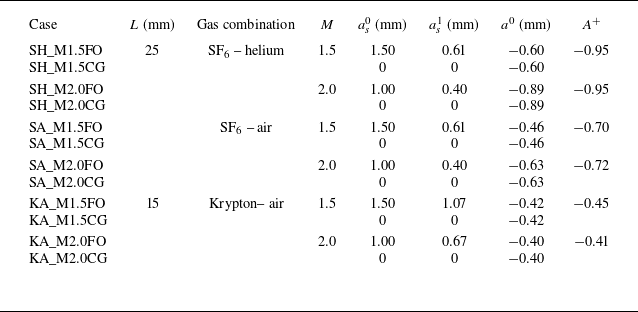
Based on (4.8)–(4.9), the freeze-out lines for varying Mach numbers and gas combinations are plotted in figure 12. To realise amplitude attenuation,
 $a_{{s}}^1$
and
 $a^0$
must lie on these freeze-out lines. We design six case–control pairs: each test case (with a rippled shock) and its corresponding control case (with a uniform shock) share identical initial interface perturbations. The initial conditions for all 12 configurations are detailed in table 3. The same approach as before was used to ensure arrival of shocks with the same strength (rippled and flat). For validation, Mach numbers 1.5 and 2.0 are selected. Lower Mach numbers are excluded because the required rippled shock amplitude
 $a_{{s}}^1$
would exceed practical limits, risking Mach stem formation on the shock front. Additionally, in krypton-based gas mixtures (denoted as ‘KA’ cases), the rapid decay of shock amplitude necessitates a reduced spacing between the rippled shock and the interface to maintain observable dynamics.
Initial parameters designed for freeze-out (‘FO’) in non-standard RMI cases and the comparison group (‘CG’) in classical RMI cases.

Figures 13(a) and 13(b) illustrate the temporal evolution of perturbation amplitude defined by crest and trough displacements (top images) and mixing width (bottom images) for the SF
 $_6$
–helium gas combination in the ‘FO’ (rippled shock) and ‘CG’ (uniform shock) cases with
 $M= 1.5$
and 2.0, respectively. Notably, in the FO cases, the perturbation amplitude stagnates, while the mixing width continues to grow. This divergence arises because higher-order harmonics are induced during shock-interface interaction. These harmonics distort the interface from sinusoidal shape, as evidenced by the interface profile embedded in figure 13. The current model focuses on fundamental mode dynamics, and successfully predicts amplitude freeze-out by balancing leading-order perturbations from the rippled shock and classical RMI. However, higher-order harmonics, generated either by shock perturbations or nonlinear RMI evolution (see figures 4 and 6), exhibit distinct growth mechanisms. Unlike the fundamental mode, these harmonics cannot be mutually cancelled, leading to persistent mixing width growth. Despite this, amplitude freeze-out in the FO cases significantly suppresses total mixing width evolution compared to the CG cases.
Comparison of amplitude and mixing width of the interface between freeze-out cases and comparison groups under different gas combinations and Mach numbers. The embedded images are the schlieren pictures at late stages for comparison.

Figures 13(c) and 13(d) illustrate the temporal evolution of perturbation amplitude (top images) and mixing width (bottom images) for the freeze-out (FO) and control (CG) cases under the SF
 $_6$
–air configuration. In the FO case, the original bubble position, subjected to the rippled shock, evolves in the reverse direction, ultimately forming a bubble-shaped spike. The quantitative trends align closely with those observed in the SF
 $ _6$
–helium combination: the amplitude stagnates, while the mixing width growth is significantly suppressed.
Figures 13(e) and 13( f) illustrate the temporal evolution of perturbation amplitude (top images) and mixing width (bottom images) for the FO and CG cases under the krypton–air configuration. Due to the low Atwood number of this gas combination, the amplitude evolution in the control group is inherently weaker. In the FO case, the original bubble evolves into a forward-propagating spike. The amplitude is only significantly suppressed in the KA_M2.0FO case. At
 $M= 1.5$
, the amplitude suppression is partial, failing to achieve full freeze-out, and the difference in mixing width between FO and CG cases is negligible. At
 $M= 2.0$
, the amplitude freeze-out in the FO case is markedly improved, accompanied by significant suppression of mixing width growth.
Overall, the new model successfully predicts the critical ratio of perturbed shock amplitude to initial interface amplitude required for amplitude freeze-out. Its predictive accuracy improves at higher Mach numbers provided that no significant Mach stems form on the shock front, and at higher Atwood numbers, where density contrasts amplify fundamental mode dominance. Once Mach stems form on the shock front, the present model loses its validity. Determining an analytical relation accounting for Mach stems remains challenging due to their non-homogeneous nature. In future work, geometrical shock dynamics (Shen et al. Reference Shen, Pullin, Samtaney and Wheatley2021; Zhang et al. Reference Zhang, Liao, Zou, Zhai, Liu and Li2024) may be used to explore localised coupling models. However, mixing width freeze-out remains unattainable at the amplitude stagnation point. This limitation stems from the divergent origins of higher-order modes: those induced by the rippled shock differ fundamentally from those generated via nonlinear evolution in classical RMI. These un-cancelled growths of higher-order modes drive persistent mixing width growth, in spite of the stagnation of fundamental mode evolution. In ICF, non-ideal effects such as viscosity, surface tension and real-gas equations of state can modify the freeze-out relationships. Viscosity and surface tension are known to exert a stabilising influence on RMI (Mikaelian Reference Mikaelian1993). As a result, these effects may broaden the freeze-out condition from a single parameter point into a narrow zone. Furthermore, the real-gas equation of state introduces a spectrum of simultaneous acoustic emissions (Andrés et al. Reference Andrés, Alexander and César2023), which could also shift the freeze-out relationships.
5. Conclusions
This paper derives the asymptotic growth rate of perturbation amplitude for non-standard Richtmyer–Meshkov instability (RMI), specifically investigating the interaction of a first-phase rippled shock with a flat or perturbed heavy–light interface. Numerical validation is performed using the HOWD code. Unlike previous models requiring empirical coefficients, our analytical framework demonstrates robustness across three scenarios: classical RMI, non-standard RMI with rippled shock impinging on flat interfaces, and non-standard RMI with perturbations presented on both shock wave and interface. We emphasise that our model provides an initial approximation of the linear growth rate for non-standard RMI induced by rippled shocks during their immediate post-generation phase, excluding the perturbation history of the shock. This formulation should therefore be considered a time-limited analytical estimation rather than a comprehensive solution. Notably, our model demonstrates efficacy in coupled perturbation systems, a prevalent condition in thin gas layer geometries where classical and non-standard RMI mechanisms exhibit maximal cross-coupling intensity.
Through analysis of the scenarios where the rippled shock and the perturbed interface have identical profiles, this study reveals that baroclinic vorticity generation in non-standard RMI originates not merely from shock-surface pressure gradients, but critically incorporates post-shock pressure gradients, a mechanism neglected in prior analyses of this type. This oversight fundamentally undermines conventional vortex models, and crucially explains the intrinsic non-equivalence between classical and non-standard RMI dynamics. Our model shows priority in predicting the asymptotic growth rate and asymptotic circulation in this situation.
The study establishes the critical criterion for perturbation freeze-out in non-standard RMI, empirically validated through numerical experiments across multiple configurations. The model demonstrates enhanced predictive accuracy with increasing Mach and Atwood numbers provided that the Mach stem is absent on the shock front. Since the mode growth of the interface perturbation in non-standard RMI differs from that in the classical RMI, higher-order perturbations on the interface continue to develop even when the amplitude at the crests and troughs is maximally suppressed, resulting in an increase in mixing width.
Funding
This work was supported by the National Natural Science Foundation of China (nos 12372281 and 12388101), the Strategic Priority Research Programme of the Chinese Academy of Sciences (no. XDB0620201) and Youth Innovation Promotion Association CAS.
Declaration of interests
The authors report no conflict of interest.
Appendix A. Background flow parameters formation
The background flow parameters are calculated with one-dimensional gas dynamics. The balanced pressure near the shocked interface
 $p_{{\! f}}$
, the interface velocity
 $\Delta \!V$
, and the Mach number of transmitted shock
 $M_{{T}}=V_{{T}}/c_{\boldsymbol{a}{0}}$
are the three unknown variables to be solved:
 \begin{equation} \begin{aligned} &\Delta \!V=\psi _u (p_1, \gamma _{\boldsymbol{a}}, \gamma _{\boldsymbol{b}}, A^-), \\ &p_{{\! f}}=\psi _p (p_1, \gamma _{\boldsymbol{a}}, \gamma _{\boldsymbol{b}}, A^-), \\ &M_{{T}}=\psi _M (p_1, \gamma _{\boldsymbol{a}}, \gamma _{\boldsymbol{b}}, A^-). \end{aligned} \end{equation}
To close the problem, three equations are needed. After the shock–interface interaction, the flow field is divided into four zones ( b 1, bf, af and a 0). Three boundary conditions are established between the neighbouring zones. The Rankine–Hugoniot relationships stand for TS separating the af and a 0 zones. The pressure and velocity hold consistency across the interface separating the af and bf zones. The isentropic relationships are established across RW separating the b 1 and bf zones. Consequently, we have
 \begin{equation} \Delta \!V/c_{\boldsymbol {a}0}=\frac {2}{\gamma _{\boldsymbol{a}}+1}\frac {M_{{T}}^2-1}{M_{{T}}}, \end{equation}
 \begin{equation} (p_{{\! f}}-p_0)/p_0=\frac {2\gamma _{\boldsymbol{a}}}{\gamma _{\boldsymbol{a}}+1}(M_{{T}}^2-1), \end{equation}
 \begin{equation} (\Delta \!V-u_{\boldsymbol{b}1})/c_{\boldsymbol{b}1}=-\frac {2}{\gamma _{\boldsymbol{b}}-1}\left[\left(\frac {p_{{\! f}}}{p_1}\right)^{(\gamma _{\boldsymbol{b}}-1)/2\gamma _{\boldsymbol{b}}}-1\right]. \end{equation}
Combining these three equations, a solution for (A1) can be derived.
Appendix B. Model degeneralisation to the classical RMI model
By setting
 $a_{{s}}^1=0$
, the model reduces to the irrotational WN model, which describes the classical RMI. Assuming
 $a_{{s}}^1=0$
in (2.19) yields
 \begin{equation} \begin{aligned} \dot {a}^\infty ={}&\frac {A^++1}{2}k\,\Delta \!V \left (1-\frac {V_{{T}}}{V_{{I}}}\right )a^0 \\&{}-\frac {A^+-1}{2}k\frac {c_{\boldsymbol{b}1}-c_{\boldsymbol{b}{\!f}}+\Delta \!V-u_{\boldsymbol{b}1}}{V_{{I}}(\gamma _{\boldsymbol{b}}+1)}(c_{\boldsymbol{b}1}-3c_{\boldsymbol{b}{\!f}}+\Delta \!V+u_{\boldsymbol{b}1}-2V_{{I}})a^0. \end{aligned} \end{equation}
By rearranging (B1) to match the form of (2.10), we obtain
 \begin{equation} \dot {a}^\infty =\frac {\rho _{\boldsymbol{a}{\!f}}\,\delta {v}_{{y}\boldsymbol{a}}^0-\rho _{\boldsymbol{b}{\!f}}\,\delta {v}_{{y}\boldsymbol{b}}^0}{\rho _{\boldsymbol{a}{\!f}}+\rho _{\boldsymbol{b}{\!f}}}, \end{equation}
where the tangential velocity
 ${v}_{{y}\boldsymbol{a}}^0$
and
 ${v}_{{y}\boldsymbol{b}}^0$
can be expressed as
 \begin{equation} {v}_{{y}\boldsymbol{a}}^0=k\,\Delta \!V \left (1-\frac {V_{{T}}}{V_{{I}}}\right )a^0, \end{equation}
 \begin{equation} {v}_{{y}\boldsymbol{b}}^0=k\frac {c_{\boldsymbol{b}1}-c_{\boldsymbol{b}{\!f}}+\Delta \!V-u_{\boldsymbol{b}1}}{V_{{I}}(\gamma _{\boldsymbol{b}}+1)}(c_{\boldsymbol{b}1}-3c_{\boldsymbol{b}{\!f}}+\Delta \!V+u_{\boldsymbol{b}1}-2V_{{I}})a^0. \end{equation}
The expression for
 ${v}_{{y}\boldsymbol{a}}^0$
is identical to the irrotational WN model for classical RMI (Wouchuk & Nishihara Reference Wouchuk and Nishihara1997; Wouchuk Reference Wouchuk2001). To calculate the tangential velocity in the fluid
b
side, we can first derive the amplitudes of the rarefaction leading edge and trailing edge:
 \begin{equation} a^0_{\textit{RL}}=a^0\frac {V_{{I}}+c_{\boldsymbol{b}1}-u_{\boldsymbol{b}1}}{V_{{I}}}, \end{equation}
 \begin{equation} a^0_{\textit{RT}}=a^0\frac {V_{{I}}+c_{\boldsymbol{b}{\!f}}-\Delta \!V}{V_{{I}}}. \end{equation}
By substituting (B5) and (B6) into (2.15), we can verify that (B4) is equivalent to the tangential velocity on the reflected side of classical RMI.