1 Introduction
Gravity currents – the predominantly horizontal motion of fluids driven by density differences – occur in many large-scale environmental and industrial settings. Examples include the spreading of dense gases in the atmosphere, the interaction between fresh and saline waters in estuaries and the transport of dilute suspension of particles along the ocean floor. The dynamics of inertially dominated (high Reynolds number) gravity currents has been explored for many decades through laboratory experiments, field observations and mathematical models that capture flow speeds and other properties as functions of the source conditions (see Simpson (Reference Simpson1997) and Ungarish (Reference Ungarish2009) for thorough presentations of flow phenomena and properties of gravity currents).
Theoretical models have adopted a number of strategies for capturing these motions, ranging from direct numerical simulation of the complete system of dynamical equations, to layer-averaged models that exploit the relative thinness of most flows, to integral models that do not resolve all of the interior characteristics. Dimensional reasoning and scaling analyses are often useful tools for probing the dynamics of the motions (though note the cautionary results of Johnson et al. (Reference Johnson, Hogg, Huppert, Sparks, Phillips, Slim and Woodhouse2015)). Very often, however, it has been demonstrated that the differing approaches nevertheless lead to similar quantitative predictions of the bulk motions (see, for example, Hogg et al. (Reference Hogg, Nasr-Azadani, Ungarish and Meiburg2016)).
A key component of shallow layer and integral models is the dynamical condition that links the flow speed and the flow depth at the front of the current, where the pressure is non-hydrostatic due to the significant vertical velocities that develop as the displaced environmental fluid is uplifted over the advancing head of the relatively dense fluid. This condition, often termed the ‘Froude number’ condition, closes the model description and thus plays a vital role in the predictions of the flow speeds. Von Kármán (Reference Von Kármán1940) produced one of the first models for the Froude number on the basis of ideal fluid flow. His arguments were later refined and significantly improved upon by Benjamin (Reference Benjamin1968), who developed expressions for mass conservation and momentum balance over a control volume encompassing the front, while allowing for dissipation. More recently Borden & Meiburg (Reference Borden and Meiburg2013a ) and Konopliv et al. (Reference Konopliv, Llewellyn-Smith, McElwaine and Meiburg2016) have produced models based upon the conservation of vorticity (or ‘circulation’) over the frontal control volume, establishing expressions for the Froude number that are close to, but in general not identical to, Benjamin’s result.
These, and other previous investigations, have invested considerable efforts in addressing which of the many ‘formally correct’ solutions of the mathematical idealisations of the flow dynamics is the most appropriate model. The major tool of assessment was comparison of the front speed (or Froude number) with experiments and Navier–Stokes simulations, alongside qualitative arguments concerning the energy dissipation. Such justifications based upon ‘bulk’ properties may be problematic since they examine integral measures of the motion rather than the detailed velocity fields. Furthermore data are relatively scarce and generally, but not exclusively, limited to the Boussinesq regime with equal fluid viscosities. Models have also often examined laminar steady states with free-slip boundaries in the limit of vanishing solute diffusivity – and these regimes are usually not in accord with laboratory experiments or numerical simulations of the fluid motions.
The purpose of this contribution is to revisit the derivation of the Froude number and to show how the results of Benjamin (Reference Benjamin1968) and Borden & Meiburg (Reference Borden and Meiburg2013a ) can be reconciled within the same theoretical framework. This is important because both analyses start from the same configuration and governing equations – namely two-layer high Reynolds number flow – and yet appear to diverge somewhat in their results. We demonstrate that both results arise from the same control volume formulation and we highlight that it is different assumptions (explicit or implicit) that lead to the differences in their results. Indeed, we show that within the context of two-layer fluid flow with free-slip boundaries, which is the starting point for both, they differ in their assumptions about the dissipation in the system. This is curious since both approaches appear to be based upon inviscid models of the motion and viscosity does not enter explicitly in the final results for front speed or energy dissipation. However the ‘inviscid’ model is an illusion – the non-vanishing dissipation can only be justified if the derivation is based upon the Navier–Stokes equations. Also it is noteworthy that although the motion sufficiently far upstream of the front may be irrotational, the flow around the front is certainly rotational.
In this contribution we also explore the consequences of including shear in the model of velocity field behind the front of the current or a bore, a feature that is excluded by traditional two-layer hydraulic models for which the vorticity is concentrated to a velocity discontinuity between the flowing layers. A continuous transition layer has been considered briefly by previous studies (Klemp, Rotunno & Skamarock Reference Klemp, Rotunno and Skamarock1994, Borden, Meiburg & Constantinescu Reference Borden, Meiburg and Constantinescu2012b , Borden & Meiburg Reference Borden and Meiburg2013a ,Reference Borden and Meiburg b , Baines Reference Baines2016). Here we apply the idea of a ‘wake’ in a more systematic way, which is based on the governing equations and avoids the use of empirical data and adjustable constants (Borden et al. Reference Borden, Meiburg and Constantinescu2012b ; Borden & Meiburg Reference Borden and Meiburg2013a ,Reference Borden and Meiburg b ; Baines Reference Baines2016) and the need for linearisation (Klemp et al. Reference Klemp, Rotunno and Skamarock1994). We show that by harnessing conservation of mass and momentum balance, together with a model of the velocity wake, we may develop a new class of models for the Froude number, which are quantitatively in line with existing experimental and simulation data and which compute the thickness of the rotational region as an intrinsic part of the solution. We term this class as ‘vortex-wake’ models, as opposed to the ‘vortex-sheet’ model of Benjamin and others.
Our analysis may also be applied to jumps (bores) within horizontal, two-layer stratified flows. Models of the velocity of bores within this context have crucially depended upon assumptions about the dissipation (see Wood & Simpson (Reference Wood and Simpson1984), Klemp, Rotunno & Skamarock (Reference Klemp, Rotunno and Skamarock1997), Li & Cummins (Reference Li and Cummins1998) and Baines (Reference Baines2016)). Here we develop a unifying framework and demonstrate that analysis of the vorticity balance within the flow leads to way of constraining the closure assumptions which yields a sharper criterion than the analysis of the energetics of the motion. We also present a new model that exploits a description of the wake downstream of the bore.
The structure of the paper is as follows. In § 2 we introduce the system, boundary conditions and some general equations which are the basis of the unified theory. In § 3 we revisit the gravity current problem. We present solutions for both the classical, vortex-sheet formulation and the new, vortex-wake model. The analysis supports the results of Benjamin (Reference Benjamin1968) for the dimensionless speed of the front of the current (encompassed as the Froude number,
 $Fr$
), and also provides a novel analytical expression for
 $Fr$
which emerges from the new vortex-wake formulation. Internal jumps are revisited in § 4. The classical models in the context of two-layer hydraulics are based upon a vortex-sheet model of the velocity field, which has a discontinuous velocity field at the density interface (see Wood & Simpson Reference Wood and Simpson1984; Klemp et al.
Reference Klemp, Rotunno and Skamarock1997; Borden & Meiburg Reference Borden and Meiburg2013a
; Baines Reference Baines2016) and these are considered in § 4.1, where it is demonstrated that the models based upon the conservation of circulation fall into the same analytical framework. Then in § 4.2 we solve the vortex-wake model and compare results with both existing formulae and previously published numerical data. We summarise and make some concluding remarks in § 5. This paper also includes two appendices. In the first (appendix A), we demonstrate the equivalence between an expression of vorticity conservation over the control volume encompassing the front and the requirement that the pressure field is single-valued, given that it is constructed to be hydrostatic far from the front or jump. In appendix B, we calculate the speed of the internal jump using the new vortex-wake model with an alternative velocity profile.
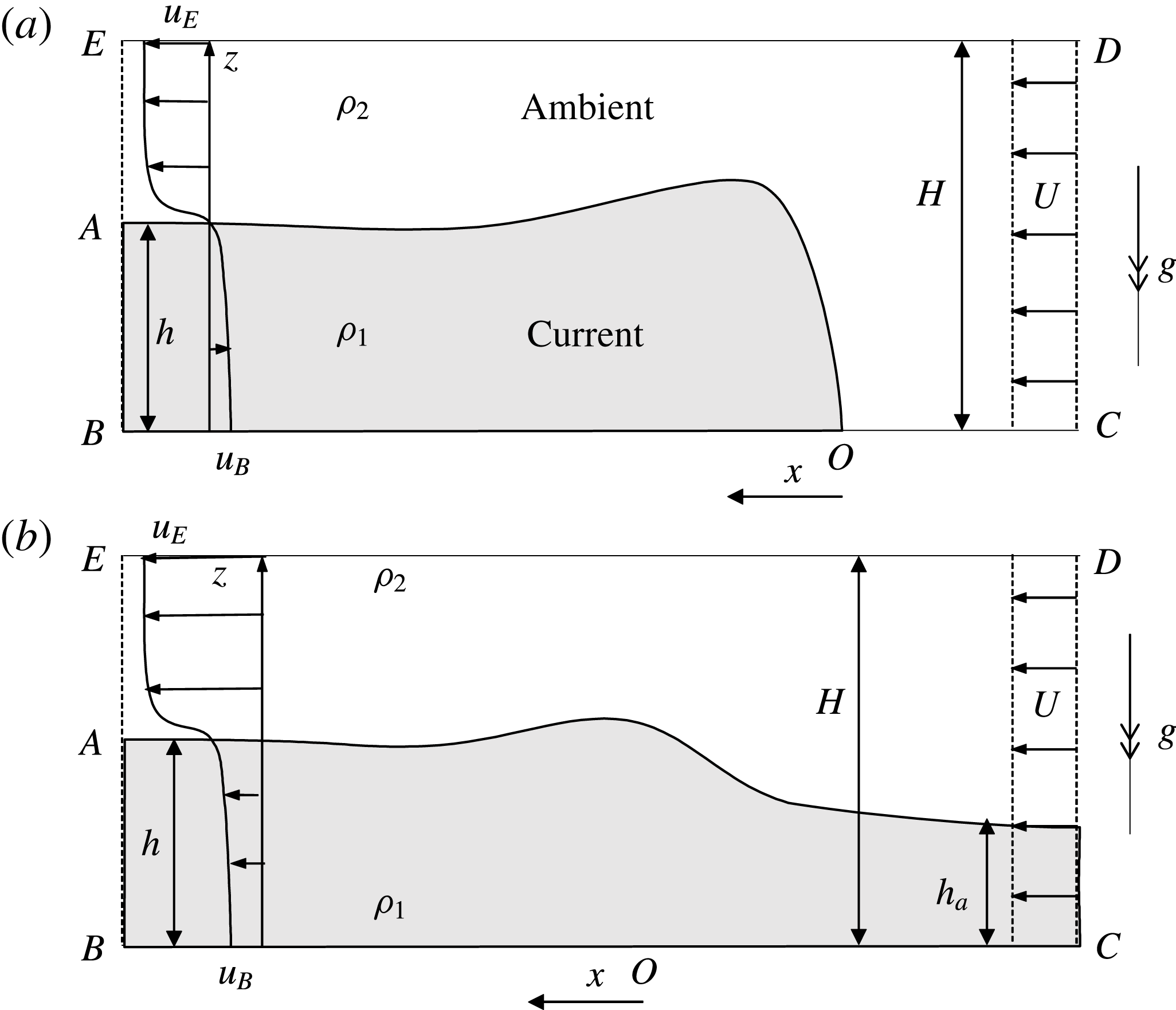
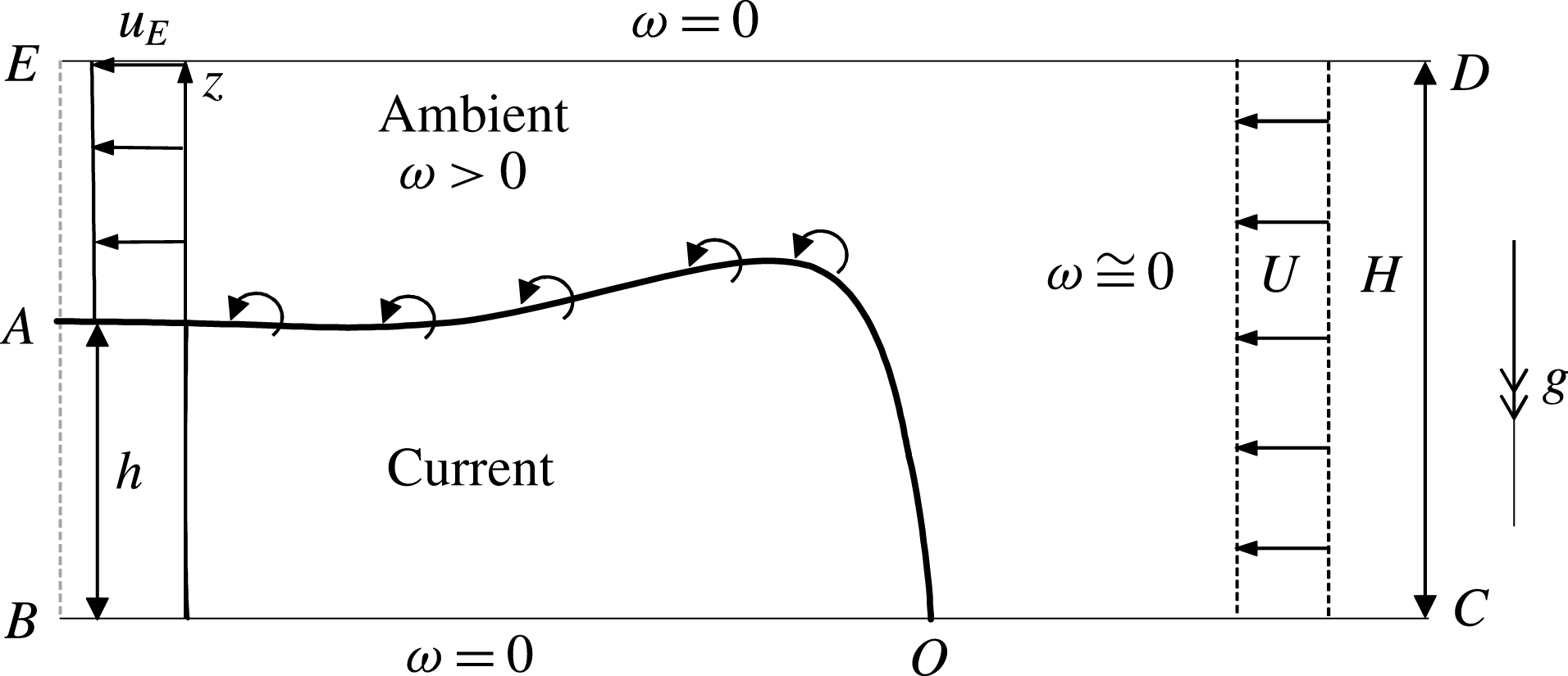
Schematic of (a) the front of a gravity current and (b) an internal jump, with the control volume
 $ABCDE$
. The current and jump are depicted in a frame of reference in which the front and jump are stationary and the fluid flows towards them with speed
 $U$
.

2 Governing equations
We examine the motion of either a gravity current of density
 $\unicode[STIX]{x1D70C}_{1}$
advancing into otherwise quiescent fluid of constant density,
 $\unicode[STIX]{x1D70C}_{2}$
(see figure 1
a) or an internal jump advancing into quiescent fluid stratified into two horizontal layers of density
 $\unicode[STIX]{x1D70C}_{1}$
and
 $\unicode[STIX]{x1D70C}_{2}$
, with
 $\unicode[STIX]{x1D70C}_{1}>\unicode[STIX]{x1D70C}_{2}$
(see figure 1
b). The motion occurs within a horizontal channel with rigid boundaries separated by distance
 $H$
. It is convenient to work in a frame of reference in which the front of the current or the internal jump is motionless and so the ambient fluid is oncoming with speed
 $U$
(see figure 1). The analysis is two-dimensional and the coordinate axes are
 $x$
(horizontal and aligned with oncoming flow) and
 $z$
(vertical and upwards), with unit vectors
 $\hat{\boldsymbol{x}}$
and
 $\hat{\boldsymbol{z}}$
, respectively. The control volume
 $ABCDE$
encloses the front or jump (see figure 1), with its edges
 $CD$
and
 $BE$
sufficiently distant so that the velocity field across these edges is parallel to the
 $x$
-axis. The origin is located at the stagnation point of the gravity current, which demarks the location of the interface between the dense fluids at the lower boundary and at the position of the internal jump where the overlying less dense fluid undergoes significant contraction. The interface height,
 $h$
, at the section
 $BE$
corresponds to the elevation at which the density of the fluid corresponds to the mean density
 $((\unicode[STIX]{x1D70C}_{1}+\unicode[STIX]{x1D70C}_{2})/2)$
, or if the density field is assumed to be discontinuous, the height of the dense fluid layer.
We assume that the motion is steady in the moving frame of reference and thus neglect both transient effects, as the flow is established, and the potential for wave-induced transport. Many studies have demonstrated that the bulk properties of gravity currents and internal jumps are steady if, for example, the motion is generated by a sustained, constant flux or during the initial phases of ‘lock release’ (Ungarish Reference Ungarish2009). Additionally, Ungarish (Reference Ungarish2009) argued that even for unsteady flows, a local analysis within a control volume spanning and moving with the front or jump features steady dynamics. Unsteady (undular) wave generation from internal jumps have been shown to arise when the height of the jump relative to the height of the oncoming dense fluid is small, and to be more prevalent when the relative density difference,
 $(\unicode[STIX]{x1D70C}_{1}-\unicode[STIX]{x1D70C}_{2})/\unicode[STIX]{x1D70C}_{2}$
, is of order unity (Borden, Koblitz & Meiburg Reference Borden, Koblitz and Meiburg2012a
). This unsteady mechanism is not included in what follows, and this excludes a small subdomain from the wide domain of parameters (height and density ratios) covered by our analysis.
The equations of steady-state motion are
 $$\begin{eqnarray}\displaystyle & \displaystyle \unicode[STIX]{x1D735}\boldsymbol{\cdot }\boldsymbol{u}=0, & \displaystyle\end{eqnarray}$$
 $$\begin{eqnarray}\displaystyle & \displaystyle \boldsymbol{u}\boldsymbol{\cdot }\unicode[STIX]{x1D735}\boldsymbol{u}=-\frac{1}{\unicode[STIX]{x1D70C}}\unicode[STIX]{x1D735}p-g\hat{\boldsymbol{z}}+\frac{1}{\unicode[STIX]{x1D70C}}\unicode[STIX]{x1D735}\boldsymbol{\cdot }\unicode[STIX]{x1D749}. & \displaystyle\end{eqnarray}$$
Here
 $\boldsymbol{u}=(u,w)$
is the velocity field,
 $p$
is the pressure,
 $\unicode[STIX]{x1D749}$
is the deviatoric stress tensor and
 $-g\hat{\boldsymbol{z}}$
is acceleration due to gravity. Since the velocity field is two-dimensional, the vorticity field is aligned with the
 $y$
-axis and is given by
 $\unicode[STIX]{x1D714}\hat{\boldsymbol{y}}$
, where
 $$\begin{eqnarray}\unicode[STIX]{x1D714}=\frac{\unicode[STIX]{x2202}u}{\unicode[STIX]{x2202}z}-\frac{\unicode[STIX]{x2202}w}{\unicode[STIX]{x2202}x}.\end{eqnarray}$$
We note that the divergence of the stress may be written
 $$\begin{eqnarray}\unicode[STIX]{x1D735}\boldsymbol{\cdot }\unicode[STIX]{x1D749}=-\unicode[STIX]{x1D707}\unicode[STIX]{x1D735}\wedge (\unicode[STIX]{x1D735}\wedge \boldsymbol{u})=\unicode[STIX]{x1D707}\left(\frac{\unicode[STIX]{x2202}\unicode[STIX]{x1D714}}{\unicode[STIX]{x2202}z}\hat{\boldsymbol{x}}-\frac{\unicode[STIX]{x2202}\unicode[STIX]{x1D714}}{\unicode[STIX]{x2202}x}\hat{\boldsymbol{z}}\right),\end{eqnarray}$$
where
 $\unicode[STIX]{x1D707}$
is the dynamic viscosity, which is assumed constant. This identity is used below (see (2.18) and (2.19)). The pressure
 $p(x,z)$
must be a single-valued function and consequently
 $\unicode[STIX]{x1D735}\wedge \unicode[STIX]{x1D735}p=\mathbf{0}$
in the flow domain. Then integrating over the surface spanning
 $ABCDE$
with unit normal
 $\hat{\boldsymbol{y}}$
, which is bounded by the directed curve
 $\unicode[STIX]{x1D6E4}=ABCDE$
, must give
 $$\begin{eqnarray}0=\int _{S}\unicode[STIX]{x1D735}\wedge \unicode[STIX]{x1D735}p\boldsymbol{\cdot }\hat{\boldsymbol{y}}\,\text{d}S=\oint _{\unicode[STIX]{x1D6E4}}\unicode[STIX]{x1D735}p\boldsymbol{\cdot }\,\text{d}\boldsymbol{x}.\end{eqnarray}$$
The conditions on the boundary of the control volume are as follows. The upstream flow corresponds to uniform velocity
 $\boldsymbol{u}=U\hat{\boldsymbol{x}}$
. The downstream flow is parallel to the channel boundaries, which are horizontal, and the velocity field at
 $BE$
is denoted by
 $\boldsymbol{u}=u(z)\hat{\boldsymbol{x}}$
. The boundaries
 $BC$
 $(z=0)$
and
 $DE$
 $(z=H)$
are impermeable and stress-free; thus
 $w=0$
and
 $\unicode[STIX]{x2202}u/\unicode[STIX]{x2202}z=0$
. Importantly these are not inviscid boundary conditions and do not preclude the possibility of viscous dissipation as shown below. We note immediately that together these boundary conditions imply that the vertical component of the velocity field,
 $w$
, vanishes on all of the boundary,
 $\unicode[STIX]{x1D6E4}$
. Furthermore these conditions imply that vorticity,
 $\unicode[STIX]{x1D714}$
, vanishes on the free-slip boundaries
 $(BC,DE)$
and on the inflow
 $(CD)$
, whereas it is non-vanishing on the outflow. Finally there is stress and velocity continuity at the interface between the fluids of differing density (i.e. at
 $z=h$
on
 $BE$
).
2.1 Pressure field
As a consequence of assumed parallel flow on the inflow and outflow, the pressure adopts hydrostatic balance over the section
 $BAE$
and
 $CD$
, and is given by
 $$\begin{eqnarray}\frac{\unicode[STIX]{x2202}p}{\unicode[STIX]{x2202}z}=-(\unicode[STIX]{x1D70C}_{2}+\unicode[STIX]{x0394}\unicode[STIX]{x1D70C}(z))g,\end{eqnarray}$$
where the density of the fluid is written
 $\unicode[STIX]{x1D70C}(z)=\unicode[STIX]{x1D70C}_{2}+\unicode[STIX]{x0394}\unicode[STIX]{x1D70C}(z)$
and thus
 $\unicode[STIX]{x0394}\unicode[STIX]{x1D70C}$
is the excess density. Upstream we denote the depth of the dense fluid by
 $h_{a}$
, noting that for a gravity current
 $h_{a}$
vanishes. The pressure distribution on
 $CD$
is then given by
 $$\begin{eqnarray}p=\left\{\begin{array}{@{}ll@{}}p_{D}+\unicode[STIX]{x1D70C}_{2}g(H-z),\quad & h_{a}<z<H,\\ p_{D}+\unicode[STIX]{x1D70C}_{2}g(H-h_{a})+\unicode[STIX]{x1D70C}_{1}g(h_{a}-z),\quad & 0<z<h_{a},\end{array}\right.\end{eqnarray}$$
while the pressure distribution on
 $BE$
is given by
 $$\begin{eqnarray}p=p_{E}+\int _{0}^{H}(\unicode[STIX]{x1D70C}_{2}+\unicode[STIX]{x0394}\unicode[STIX]{x1D70C})g\;\text{d}z.\end{eqnarray}$$
In this integral (2.8), and throughout,
 $z$
-integrals are evaluated over the outflow boundary
 $BAE$
. It is then straightforward to evaluate the differences in pressure between the upper and lower boundaries at these inflow and outflow locations. These are given by
 $$\begin{eqnarray}\displaystyle & \displaystyle p_{C}-p_{D}=\unicode[STIX]{x1D70C}_{2}gH+(\unicode[STIX]{x1D70C}_{1}-\unicode[STIX]{x1D70C}_{2})gh_{a}, & \displaystyle\end{eqnarray}$$
 $$\begin{eqnarray}\displaystyle & \displaystyle p_{B}-p_{E}=\unicode[STIX]{x1D70C}_{2}gH+\int _{0}^{H}\unicode[STIX]{x0394}\unicode[STIX]{x1D70C}g\;\text{d}z. & \displaystyle\end{eqnarray}$$
The pressure differences on
 $BC$
and
 $DE$
may be expressed from (2.2), noting that
 $w=0$
on these boundaries. On
 $DE$
this yields
 $$\begin{eqnarray}\frac{\unicode[STIX]{x1D70C}_{2}u_{E}^{2}}{2}+p_{E}=\frac{\unicode[STIX]{x1D70C}_{2}U^{2}}{2}+p_{D}+\int _{D}^{E}\unicode[STIX]{x1D707}\unicode[STIX]{x1D6FB}^{2}u\;\text{d}x,\end{eqnarray}$$
while on
 $BC$
 $$\begin{eqnarray}\frac{\unicode[STIX]{x1D70C}_{1}u_{B}^{2}}{2}+p_{B}+\int _{B}^{O}\unicode[STIX]{x1D707}\unicode[STIX]{x1D6FB}^{2}u\;\text{d}x=\frac{\unicode[STIX]{x1D70C}_{C}U^{2}}{2}+p_{C}+\int _{C}^{O}\unicode[STIX]{x1D707}\unicode[STIX]{x1D6FB}^{2}u\;\text{d}x,\end{eqnarray}$$
where
 $\unicode[STIX]{x1D70C}_{C}$
is the density at
 $C$
(which is equal to
 $\unicode[STIX]{x1D70C}_{2}$
for the gravity current scenario and
 $\unicode[STIX]{x1D70C}_{1}$
for internal jumps). Also in the latter expression we have separated the dissipative effects into contributions from
 $OB$
and
 $OC$
.
We may now combine these expressions for the pressure differences over the boundaries of the control volume to satisfy the requirement that the pressure field is single-valued (2.5). Thus evaluating
 $(p_{C}-p_{D})+(p_{D}-p_{E})+(p_{E}-p_{B})+(p_{B}-p_{C})=0$
from (2.9)–(2.12), we deduce that
 $$\begin{eqnarray}\displaystyle & & \displaystyle \frac{\unicode[STIX]{x1D70C}_{2}u_{E}^{2}}{2}-\frac{\unicode[STIX]{x1D70C}_{1}u_{B}^{2}}{2}-\frac{U^{2}}{2}(\unicode[STIX]{x1D70C}_{2}-\unicode[STIX]{x1D70C}_{C})=\int _{0}^{H}\unicode[STIX]{x0394}\unicode[STIX]{x1D70C}g\;\text{d}z-(\unicode[STIX]{x1D70C}_{1}-\unicode[STIX]{x1D70C}_{2})gh_{a}\nonumber\\ \displaystyle & & \displaystyle \quad +\,\int _{D}^{E}\unicode[STIX]{x1D707}\unicode[STIX]{x1D6FB}^{2}u\;\text{d}x-\int _{C}^{O}\unicode[STIX]{x1D707}\unicode[STIX]{x1D6FB}^{2}u\;\text{d}x-\int _{O}^{B}\unicode[STIX]{x1D707}\unicode[STIX]{x1D6FB}^{2}u\;\text{d}x.\end{eqnarray}$$
It is shown in appendix A that integration of the vorticity equation over the control volume leads to an identical condition, as it must, since they are derived from the same fundamental governing principles.
2.2 Global mass and momentum balances
Mass conservation is given by
 $$\begin{eqnarray}\int _{0}^{H}u\;\text{d}z=UH,\end{eqnarray}$$
while conservation of the dense solute is given by
 $$\begin{eqnarray}\int _{0}^{H}\unicode[STIX]{x0394}\unicode[STIX]{x1D70C}\;u\;\text{d}z=(\unicode[STIX]{x1D70C}_{1}-\unicode[STIX]{x1D70C}_{2})Uh_{a}.\end{eqnarray}$$
Since there are no
 $x$
-components of the stress tensor on the boundary of the control volume, the global balance of linear momentum along the
 $x$
-axis integrated over the domain is given by
 $$\begin{eqnarray}(p_{D}-p_{E})H+\unicode[STIX]{x1D70C}_{2}U^{2}(H-h_{a})+\unicode[STIX]{x1D70C}_{1}U^{2}h_{a}-\int _{0}^{H}\unicode[STIX]{x1D70C}u^{2}\;\text{d}z=\int _{0}^{H}z\unicode[STIX]{x0394}\unicode[STIX]{x1D70C}g\;\text{d}z-\frac{1}{2}(\unicode[STIX]{x1D70C}_{1}-\unicode[STIX]{x1D70C}_{2})gh_{a}^{2}.\end{eqnarray}$$
We emphasise that this balance, which is sometimes termed the ‘flow force balance’, does not explicitly include the effects of viscosity due to the assumed conditions on the boundary of the control volume. This does not imply that viscous effects are absent within the control volume. Indeed an inviscid analysis would eliminate coupling between the flowing layers and energy dissipation, assumptions that restrict the results to a very narrow range of parameter values. Some recent studies (Borden et al. Reference Borden, Meiburg and Constantinescu2012b , Borden & Meiburg Reference Borden and Meiburg2013a ,Reference Borden and Meiburg b , Konopliv et al. Reference Konopliv, Llewellyn-Smith, McElwaine and Meiburg2016) suggested that vorticity conservation for the control volume should be added to the formulation. However, as explained above and demonstrated in appendix A, this condition is equivalent to the requirement that the pressure field is single-valued and is embodied in (2.5) and (2.13).
The formulation above is the common basis for various models that predict the velocities of the front of gravity currents and of internal jumps,
 $U$
(and some related features, such as energy dissipation). For both flow problems, closure assumptions specify the outflow velocity and density profiles (
 $u(z)$
and
 $\unicode[STIX]{x0394}\unicode[STIX]{x1D70C}(z)$
, respectively) and usually some additional assumptions are made about the energy dissipation or the source of vorticity. Then this framework yields an expression for the speed,
 $U$
, expressed dimensionlessly in terms of a Froude number, as a function of the relative depth of the dense fluid layer. Very often the outflow velocity is assumed to be piecewise constant in the layers with a discontinuity of velocity at the interface (i.e. a vortex sheet), but an alternative model pursued in this study features a velocity profile in which the velocity transitions between the layers over a finite thickness, denoted by
 $\unicode[STIX]{x1D702}$
, the magnitude of which emerges from the model. We term this latter class of models as ‘vortex-wake’ models, because the velocity field in the wake of the front or the jump is rotational. We note that although these approaches are related, the vortex-sheet model does not emerge as the limit of vanishing thickness of the vortex-wake model
 $(\unicode[STIX]{x1D702}\rightarrow 0)$
, because the thickness is part of the solution and not a free variable. The models coincide only in the special case for which
 $\unicode[STIX]{x1D702}=0$
is a solution and this corresponds to an energy conserving flow.
In what follows (§§ 3 and 4), we analyse the prediction from this framework for the flow in two configurations, namely the front of gravity currents and internal jumps. For each we show that a solution may be calculated on the basis of a vortex-sheet or vortex-wake idealisation for the motion. We note that these differing approaches invoke differing assumptions about the energy losses and/or diffusion of vorticity and they diverge somewhat from each other. The challenge is to reveal the conditions for agreement, because both models approximate the same physical problem. We further note that in the Boussinesq regime
 $((\unicode[STIX]{x1D70C}_{2}-\unicode[STIX]{x1D70C}_{1})/\unicode[STIX]{x1D70C}_{2}\ll 1)$
, the vortex-sheet problem for an internal jump coincides with the problem for a gravity current in the limit
 $h_{a}/H\rightarrow 0$
. In that case, the lower layer expands strongly, and hence
 $u_{B}/U\rightarrow 0$
(as for the gravity current problem). However, in the gravity current model, the stagnation pressure at
 $O$
is proportional to upper fluid density,
 $\unicode[STIX]{x1D70C}_{2}$
, and this makes a difference for the non-Boussinesq analysis. Therefore, in general, we need separate solutions for the gravity currents and internal jumps.
2.3 Dimensionless variables and governing equations
At this point it is convenient to introduce dimensionless variables. We scale lengths with respect to the channel height
 $H$
, velocities with respect to oncoming speed
 $U$
and densities with respect to the density of the less dense fluid,
 $\unicode[STIX]{x1D70C}_{2}$
. There are five dimensionless quantities. The Froude number,
 $Fr$
, and excess density ratio,
 $S$
, are given by
 $$\begin{eqnarray}Fr^{2}=\frac{U^{2}}{g^{\prime }h}\quad \text{and}\quad S=\frac{\unicode[STIX]{x1D70C}_{1}-\unicode[STIX]{x1D70C}_{2}}{\unicode[STIX]{x1D70C}_{2}},\end{eqnarray}$$
where the reduced gravity
 $g^{\prime }=Sg$
and we define
 $\unicode[STIX]{x0394}\unicode[STIX]{x1D70C}(z)/\unicode[STIX]{x1D70C}_{2}=S\;r(z)$
. There are also two dimensionless parameters that measure the dissipation along the channel boundaries. On the streamlines
 $DE$
and
 $BC$
, noting the independence of the velocity field to the streamwise coordinate at the outflow and inflow, we write
 $$\begin{eqnarray}\displaystyle & \displaystyle \unicode[STIX]{x1D70C}_{2}g^{\prime }h\unicode[STIX]{x1D6FF}_{t}\equiv -\int _{D}^{E}\unicode[STIX]{x1D707}\unicode[STIX]{x1D6FB}^{2}u\;\text{d}x=-\int _{D}^{E}\unicode[STIX]{x1D707}\frac{\unicode[STIX]{x2202}^{2}u}{\unicode[STIX]{x2202}z^{2}}\;\text{d}x\equiv -\int _{D}^{E}\unicode[STIX]{x1D707}\frac{\unicode[STIX]{x2202}\unicode[STIX]{x1D714}}{\unicode[STIX]{x2202}z}\;\text{d}x, & \displaystyle\end{eqnarray}$$
 $$\begin{eqnarray}\displaystyle & \displaystyle \unicode[STIX]{x1D70C}_{2}g^{\prime }h\unicode[STIX]{x1D6FF}_{b}\equiv -\int _{C}^{B}\unicode[STIX]{x1D707}\unicode[STIX]{x1D6FB}^{2}u\;\text{d}x=-\int _{C}^{B}\unicode[STIX]{x1D707}\frac{\unicode[STIX]{x2202}^{2}u}{\unicode[STIX]{x2202}z^{2}}\;\text{d}x\equiv -\int _{C}^{B}\unicode[STIX]{x1D707}\frac{\unicode[STIX]{x2202}\unicode[STIX]{x1D714}}{\unicode[STIX]{x2202}z}\;\text{d}x, & \displaystyle\end{eqnarray}$$
where in (2.18) the viscosity corresponds to that of the less dense fluid, while in (2.19) it corresponds to that of the fluid along
 $BC$
(see figure 1). The dimensionless parameters,
 $\unicode[STIX]{x1D6FF}_{t}$
and
 $\unicode[STIX]{x1D6FF}_{b}$
measure the head loss on the streamlines
 $DE$
and
 $BC$
, respectively. Equivalently they measure the diffusion of vorticity from the boundaries into the flow. Additionally the parameter
 $R=\unicode[STIX]{x1D70C}_{C}/\unicode[STIX]{x1D70C}_{2}$
, which equals
 $1$
for gravity currents and
 $1+S$
for internal jumps. Henceforth all variables will be assumed to be dimensionless; in particular the scaled downstream interface height varies between zero and unity
 $(0\leqslant h\leqslant 1)$
.
The balances over the control volume have yielded four independent expressions that must be satisfied by the motion. These are conservation of mass (2.14) and dense species (2.15), the consistency of the pressure distribution to ensure that it is single-valued (2.13) and the balance of streamwise momentum (2.16), which we simplify by substituting (2.11) and (2.18) for the pressure difference
 $p_{D}-p_{E}$
. In dimensionless form these are given by
 $$\begin{eqnarray}\displaystyle & \displaystyle \int _{0}^{1}u\;\text{d}z=1, & \displaystyle\end{eqnarray}$$
 $$\begin{eqnarray}\displaystyle & \displaystyle \int _{0}^{1}ru\;\text{d}z=h_{a}, & \displaystyle\end{eqnarray}$$
 $$\begin{eqnarray}\displaystyle & \displaystyle \frac{Fr^{2}}{2}(u_{E}^{2}-(1+S)u_{B}^{2}-(1-R))=\frac{1}{h}\left(\int _{0}^{1}r\;\text{d}z-h_{a}\right)-\unicode[STIX]{x1D6FF}_{t}+\unicode[STIX]{x1D6FF}_{b}, & \displaystyle\end{eqnarray}$$
 $$\begin{eqnarray}\displaystyle & \displaystyle Fr^{2}\left(\frac{u_{E}^{2}}{2}-\int _{0}^{1}(1+Sr)u^{2}\;\text{d}z+\frac{1}{2}+Sh_{a}\right)+\unicode[STIX]{x1D6FF}_{t}=\frac{1}{h}\left(\int _{0}^{1}zr\;\text{d}z-\frac{h_{a}^{2}}{2}\right). & \displaystyle\end{eqnarray}$$
Finally we comment that in §§ 3 and 4, we will compute the rate of dissipation within the flow, denoted by
 $\dot{{\mathcal{D}}}$
and rendered dimensionless with respect to
 $\unicode[STIX]{x1D70C}_{2}(g^{\prime }h)^{3/2}h$
.
3 Gravity currents
We now specialise to find the conditions at the front of a gravity current (see figure 1
a). The interface touches the lower boundary at the stagnation point
 $O$
inside the control volume, and there is only fluid of density
 $\unicode[STIX]{x1D70C}_{2}$
in the upstream domain. This means that we set
 $h_{a}=0$
and
 $R=1$
. Moreover we consider a regime in which there is negligible mixing of the solute between the layers and the dense fluid is stationary in the frame moving with the front of the current. We do, however, account for shear in the less dense fluid across the outflow boundary
 $(AE)$
. Thus we impose
 $$\begin{eqnarray}u=u_{E}(1-f(z)),\end{eqnarray}$$
together with
 $$\begin{eqnarray}r(z)=\left\{\begin{array}{@{}ll@{}}1,\quad & 0\geqslant z<h\\ 0,\quad & h\geqslant z\geqslant 1\end{array}\right.\quad \text{and}\quad f(z)=\left\{\begin{array}{@{}ll@{}}1,\quad & 0\leqslant z\leqslant h\\ \unicode[STIX]{x1D719}((z-h)/\unicode[STIX]{x1D702}),\quad & h\leqslant z\leqslant 1,\end{array}\right.\end{eqnarray}$$
where guided by physical considerations, we assume that
 $\unicode[STIX]{x1D719}(s)$
is a continuous, monotonically decreasing function, defined for
 $s\equiv (z-h)/\unicode[STIX]{x1D702}\geqslant 0$
. Furthermore,
 $\unicode[STIX]{x1D719}(0)=1$
to ensure the velocity field is continuous at the interface
 $z=h$
and
 $\unicode[STIX]{x1D719}(s)=0$
for
 $s\geqslant 1$
, which indicates that
 $\unicode[STIX]{x1D702}$
is the thickness of the transition zone. The justification for adopting this velocity profile is that it represents simply the velocity deficit in the ambient fluid in the wake of the front of the gravity current. Furthermore it is a straightforward generalisation of the vortex-sheet model (with piecewise constant velocity fields), while maintaining a stationary layer of dense fluid. An immediate consequence of these assumed profiles is that the balance of solute (2.21) is automatically satisfied.
The pressure consistency condition (2.22) is given by
 $$\begin{eqnarray}\frac{Fr^{2}}{2}u_{E}^{2}=1+\unicode[STIX]{x1D6FF}_{b}-\unicode[STIX]{x1D6FF}_{t}.\end{eqnarray}$$
As shown in appendix A, this balance also emerges from a consideration of the vorticity; it expresses the outflow of vorticity, the baroclinic torque (which generates vorticity) and the diffusion of vorticity from the boundary. It is noteworthy that this balance emerges independently of the assumed profile on the outflow; the left-hand side of (2.22) and (3.3) is due solely to the advection of vorticity
 $u\unicode[STIX]{x1D714}=\unicode[STIX]{x2202}(u^{2}/2)/\unicode[STIX]{x2202}z$
integrated over
 $BE$
.
The other dimensionless balances are dependent upon the assumed form of the outflow. The condition of mass conservation (2.20) is given by
 $$\begin{eqnarray}u_{E}\int _{0}^{1}(1-f)\;\text{d}z=1.\end{eqnarray}$$
The momentum balance (2.23) is given by
 $$\begin{eqnarray}Fr^{2}\left(\frac{u_{E}^{2}}{2}-u_{E}^{2}\int _{0}^{1}(1-f)^{2}\;\text{d}z+\frac{1}{2}\right)+\unicode[STIX]{x1D6FF}_{t}=\frac{h}{2}.\end{eqnarray}$$
Dissipation occurs in this flow and may be evaluated by computing the difference between the fluxes of kinetic, internal and gravitational energy entering and leaving the control volume. In dimensionless form and on substitution from (3.2), it is given by
 $$\begin{eqnarray}\dot{{\mathcal{D}}}=\frac{Fr\unicode[STIX]{x1D6FF}_{t}}{h}+\frac{Fr^{3}u_{E}^{3}\unicode[STIX]{x1D702}}{2h}\int _{0}^{1}(1-(1-\unicode[STIX]{x1D719})^{2})(1-\unicode[STIX]{x1D719})\;\text{d}z.\end{eqnarray}$$
We emphasise that this expression of energy dissipation is a direct consequence of the fundamental balances of mass and momentum fluxes. It is useful because it provides some guidelines and restrictions on the domain of validity of the solutions; in particular, only flow states with
 $\dot{{\mathcal{D}}}\geqslant 0$
are possible. Equivalently (3.6) may be derived by identifying in-flow streamlines across
 $CD$
with outflow streamlines across
 $AE$
, on each of which the head loss,
 $\unicode[STIX]{x1D6FF}(z)$
, is given by
 $$\begin{eqnarray}\unicode[STIX]{x1D6FF}(z)=\unicode[STIX]{x1D6FF}_{t}+\frac{Fr^{2}u_{E}^{2}}{2}(1-(1-f(z))^{2})\quad \text{for }h<z\leqslant 1.\end{eqnarray}$$
The dimensionless dissipation is then given by
 $$\begin{eqnarray}\dot{{\mathcal{D}}}=\frac{u_{E}Fr}{h}\int _{h}^{1}\unicode[STIX]{x1D6FF}(z)(1-f)\;\text{d}z\end{eqnarray}$$
and using (3.7), this recovers (3.6).
The governing equations have therefore formed three expressions (pressure consistency (3.3), mass conservation (3.4) and momentum balance (3.5)) for five unknowns
 $(Fr,u_{E},\unicode[STIX]{x1D6FF}_{t},\unicode[STIX]{x1D6FF}_{b},\unicode[STIX]{x1D702})$
, as well as the unknown function,
 $\unicode[STIX]{x1D719}$
, that specifies the velocity profile of the outflow. The two extra unknowns indicate that the formulation is missing equations; indeed the control volume derivation has circumvented two equations. Momentum balance is formulated for the entire control volume, rather than for each layer, with an extra expression required to determine the drag force at the interface. The objective of a reliable model, therefore, is to formulate the extra unknowns in a way that is consistent with the effects that contributed to the omitted equations. We emphasise that the missing details concern momentum transfer, rather than the energetic losses.
It is useful to eliminate
 $u_{E}$
from (3.3) and (3.5) using (3.4) and in this way we find
 $$\begin{eqnarray}Fr^{2}=2(1+\unicode[STIX]{x1D6FF}_{b}-\unicode[STIX]{x1D6FF}_{t})\left(1-\int _{0}^{1}f\;\text{d}z\right)^{2},\end{eqnarray}$$
and
 $$\begin{eqnarray}(1+\unicode[STIX]{x1D6FF}_{b}-\unicode[STIX]{x1D6FF}_{t})\left(2\int _{0}^{1}f\;\text{d}z-2\int _{0}^{1}f^{2}\;\text{d}z+\left(\int _{0}^{1}f\;\text{d}z\right)^{2}\right)+\unicode[STIX]{x1D6FF}_{t}=\frac{h}{2}.\end{eqnarray}$$
To solve (3.9) and (3.10), it is necessary to add two more equations, or conditions, concerning
 $\unicode[STIX]{x1D6FF}_{b},$
 $\unicode[STIX]{x1D6FF}_{t}$
and
 $\unicode[STIX]{x1D702}$
. These variables are associated with viscous and vorticity effects inside the control volume. Physical considerations suggest that for high Reynolds number flows there should be an ‘inviscid’ result with
 $\unicode[STIX]{x1D702}$
,
 $\unicode[STIX]{x1D6FF}_{t}$
and
 $\unicode[STIX]{x1D6FF}_{b}$
set to
 $0$
. This would provide (see (3.9)) the simple ‘ideal’ (or ‘inviscid’) result
 $$\begin{eqnarray}Fr=Fr_{I}\equiv \sqrt{2}(1-h).\end{eqnarray}$$
Unfortunately, from (3.10), which reduces to
 $h^{2}=h/2$
in this case, we deduce the strong restriction that this result is only admissible when
 $h=0$
or
 $h=1/2$
. Of these values, only
 $h=1/2$
corresponds to a physically relevant inviscid current, as derived by Benjamin (Reference Benjamin1968), which is consistent with the assumption of inviscid dynamics throughout the domain. (The other root,
 $h=0$
, corresponds to a current of fixed thickness, but the dissipation when scaled by the thickness of the current is non-vanishing in a very deep ambient (
 $h\rightarrow 0$
).) Therefore, in general, it is not possible to close the model by demanding that all of the variables
 $\unicode[STIX]{x1D6FF}_{t}$
,
 $\unicode[STIX]{x1D6FF}_{b}$
and
 $\unicode[STIX]{x1D702}$
vanish; instead some criterion must be sought to incorporate the viscous effects, even if they are weak, and this leads to net dissipation and the diffusion of vorticity. In general
 $Fr_{I}$
is the upper bound for the more realistic
 $Fr$
results as shown below. The need for ‘models’ to close the system then creates dilemmas and indicates the need for more analysis, since several models may be able to capture the behaviour of
 $Fr(h)$
in a satisfactory manner. This will be discussed below. In any case, (3.6) indicates that
 $\unicode[STIX]{x1D6FF}_{t}=0$
cannot coexist with
 $\unicode[STIX]{x1D702}=0$
in general, because this combination prohibits energy dissipation.
We observe that
 $\unicode[STIX]{x1D702}=\unicode[STIX]{x1D6FF}_{t}=\unicode[STIX]{x1D6FF}_{b}=0$
are not ‘natural’ boundary conditions that can be imposed on the Navier–Stokes system of equations with free-slip and influx–outflux conditions. Instead we reiterate that
 $\unicode[STIX]{x1D702}$
,
 $\unicode[STIX]{x1D6FF}_{t}$
and
 $\unicode[STIX]{x1D6FF}_{b}$
are associated with the simplified model that replaces the flow in the control volume. Also we comment that the unspecified
 $f(z)$
(and
 $\unicode[STIX]{x1D719}(z)$
) play only a relatively minor role in the analysis, provided it varies from
 $\unicode[STIX]{x1D719}(0)=1$
to
 $\unicode[STIX]{x1D719}(1)=0$
; tests with linear and exponential profiles, as discussed later, support this inference. It is noteworthy that the function that specifies the velocity profile,
 $\unicode[STIX]{x1D719}(z)$
, is similar to a shape factor encountered in other hydraulic flows (see, for example, Hogg & Pritchard (Reference Hogg and Pritchard2004) and Woodhouse, Phillips & Hogg (Reference Woodhouse, Phillips and Hogg2016)) and a non-vanishing thickness,
 $\unicode[STIX]{x1D702}$
indicates vortical motion.
3.1 Vortex-sheet model
 $(\unicode[STIX]{x1D702}=0)$

The classical approach specifies a constant velocity
 $u_{E}$
over
 $h<z\leqslant 1$
. This implies that
 $\unicode[STIX]{x1D719}=0$
for
 $z>h$
and corresponds to a sharp velocity transition at the interface
 $z=h$
, a vortex sheet, and thus
 $\unicode[STIX]{x1D702}=0$
. The typical members of this group of models are the work of Benjamin (Reference Benjamin1968) and the recent circulation-based solutions (Borden & Meiburg Reference Borden and Meiburg2013a
, Konopliv et al.
Reference Konopliv, Llewellyn-Smith, McElwaine and Meiburg2016).
With
 $\unicode[STIX]{x1D702}=0$
, the previous results for mass conservation (3.4), pressure compatibility (3.3) and momentum balance (3.5) (already reduced to (3.9)–(3.10)) can be expressed as follows:
 $$\begin{eqnarray}\displaystyle & \displaystyle Fr^{2}=2(1-h)^{2}(1+\unicode[STIX]{x1D6FF}_{b}-\unicode[STIX]{x1D6FF}_{t}), & \displaystyle\end{eqnarray}$$
 $$\begin{eqnarray}\displaystyle & \displaystyle \unicode[STIX]{x1D6FF}_{t}+\frac{h^{2}}{1-h^{2}}\unicode[STIX]{x1D6FF}_{b}=\frac{1}{2}h\frac{1-2h}{1-h^{2}}. & \displaystyle\end{eqnarray}$$
An important outcome (see (3.7)) is that the dimensionless head loss is constant, and equal to
 $\unicode[STIX]{x1D6FF}_{t}$
, on all the streamlines in the less dense ambient (except for the stagnation line
 $CO$
). In this setting with
 $\unicode[STIX]{x1D702}=0$
, the dimensionless dissipation is
 $\dot{{\mathcal{D}}}=Fr\unicode[STIX]{x1D6FF}_{t}/h$
(see (3.6)).
The dilemma is the choice of
 $\unicode[STIX]{x1D6FF}_{t}$
and
 $\unicode[STIX]{x1D6FF}_{b}$
. As observed above, the attempt to impose
 $\unicode[STIX]{x1D6FF}_{t}=\unicode[STIX]{x1D6FF}_{b}=0$
is compatible with (3.12)–(3.13) only at the points
 $h=0$
and
 $1/2$
. At any other value of
 $h$
, at least one of the
 $\unicode[STIX]{x1D6FF}_{t}$
and
 $\unicode[STIX]{x1D6FF}_{b}$
must be non-zero. Furthermore the attempt to set
 $\unicode[STIX]{x1D6FF}_{t}=0$
fails, because in this case (3.13) yields the unacceptable
 $\unicode[STIX]{x1D6FF}_{b}\sim 1/h$
for
 $h\ll 1$
.
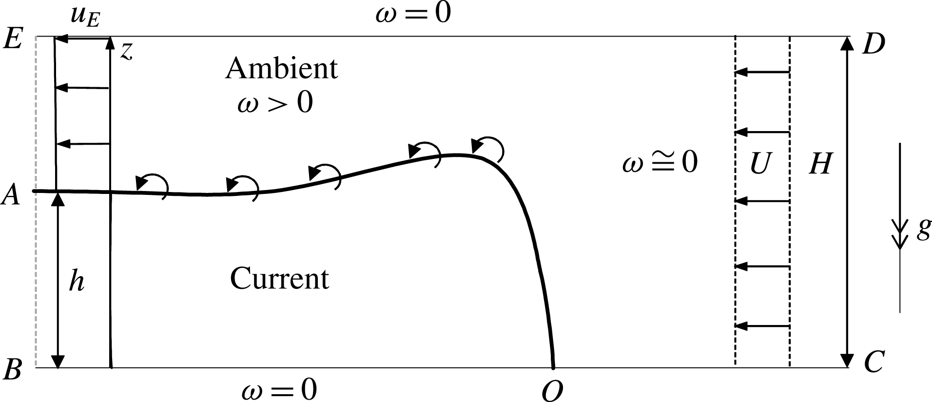
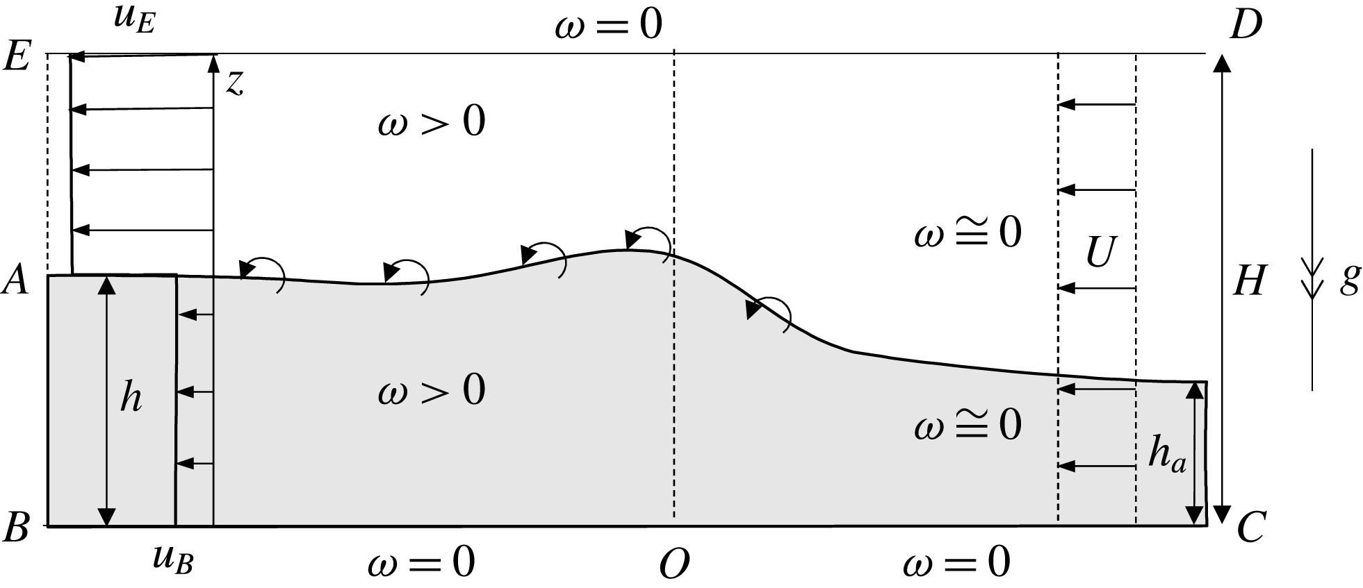
Schematic of the expected vorticity
 $\unicode[STIX]{x1D714}$
distribution in a vortex-sheet model of the flow around the front of gravity currents. In this ‘classical’ model, the vorticity vanishes
 $(\unicode[STIX]{x1D714}=0)$
on the boundaries of the control volume (
 $ABCDE$
) due to free-slip conditions and the assumptions of parallel in- and outflow, except for at the vortex sheet. Eddies are depicted to show vorticity generation at the interface between the fluids of different densities. Above the head of the current, we expect significant upward diffusion and advection of vorticity because of
 $\unicode[STIX]{x2202}\unicode[STIX]{x1D714}/\unicode[STIX]{x2202}z<0$
and the vertical component of the velocity field is non-vanishing. We expect insignificant vorticity (
 $\unicode[STIX]{x1D714}\approx 0$
) in the domain above
 $CO$
, because the inflow is uniform. This scenario demonstrates that under the ‘classical’ model it is expected that the diffusion of vorticity from the boundary
 $OC$
is much smaller than the diffusion of vorticity from
 $DE$
. Thus
 $\unicode[STIX]{x1D6FF}_{t}\gg |\unicode[STIX]{x1D6FF}_{b}|\approx 0$
in general, and this supports Benjamin’s model for the front speed with
 $\unicode[STIX]{x1D6FF}_{b}=0$
in (3.14). Note that a positive
 $\unicode[STIX]{x1D6FF}_{b}$
(as predicted by the circulation-based
 $Fr$
) requires
 $\unicode[STIX]{x1D714}<0$
above
 $OC$
.
We mentioned above that the dimensionless head losses along the boundary streamlines,
 $\unicode[STIX]{x1D6FF}_{t}$
and
 $\unicode[STIX]{x1D6FF}_{b}$
, result from flow-field features inside the control volume, and we recall the connection between
 $\unicode[STIX]{x1D6FF}_{t}$
,
 $\unicode[STIX]{x1D6FF}_{b}$
and vorticity fluxes at the top and bottom boundary (see (2.18)–(2.19)). Figure 2 shows the expected vorticity distribution. The top and bottom boundaries are free-slip with
 $\unicode[STIX]{x1D714}=0$
, the upstream flow is irrotational with
 $\unicode[STIX]{x1D714}=0$
, the dense fluid is motionless with
 $\unicode[STIX]{x1D714}=0$
. We cannot identify a mechanism that can justify the presence of a significant non-zero
 $\unicode[STIX]{x1D714}$
above the
 $CO$
line, and this implies
 $\unicode[STIX]{x2202}\unicode[STIX]{x1D714}/\unicode[STIX]{x2202}z=0$
on
 $CO$
, and hence
 $\unicode[STIX]{x1D6FF}_{b}=0$
. On the other hand,
 $\unicode[STIX]{x1D714}>0$
is expected above the interface, a gradient
 $\unicode[STIX]{x2202}\unicode[STIX]{x1D714}/\unicode[STIX]{x2202}z<0$
can be justified below the
 $DE$
boundary, and hence
 $\unicode[STIX]{x1D6FF}_{t}>0$
is the only physically consistent representation.
These observations yield simple guidelines that constrain the closure of the vortex-sheet models of gravity currents. There is no head loss on streamlines prior to contraction/expansion, i.e. upstream of
 $O$
 $(\unicode[STIX]{x1D6FF}_{b}=0)$
and the head loss in the contracting layer must be positive, in general
 $(\unicode[STIX]{x1D6FF}_{t}>0)$
. The head loss terms reduce
 $Fr$
(see (3.12)), and hence the ideal
 $Fr_{I}$
is the upper bound of this result, as expected.
These conditions
 $\unicode[STIX]{x1D6FF}_{t}>0,\unicode[STIX]{x1D6FF}_{b}=0$
lead directly to the solution due to Benjamin (Reference Benjamin1968):
 $$\begin{eqnarray}Fr^{2}=Fr_{B}^{2}\equiv \frac{(2-h)(1-h)}{1+h};\quad \unicode[STIX]{x1D6FF}_{t}=\frac{1}{2}h\frac{1-2h}{1-h^{2}}.\end{eqnarray}$$
Note that our discussion of feasible values of
 $\unicode[STIX]{x1D6FF}_{t}$
and
 $\unicode[STIX]{x1D6FF}_{b}$
was not based upon energetic considerations. Rather, we have framed the discussion in terms of vorticity. Moreover, by the same logic we infer that
 $\unicode[STIX]{x1D6FF}_{t}<0$
is not feasible, and hence the range of validity of (3.14) is
 $h\in (0,1/2]$
.
A key weakness in this argument based upon vorticity is the reliance on the presence of a significant, non-vanishing gradient
 $\unicode[STIX]{x2202}\unicode[STIX]{x1D714}/\unicode[STIX]{x2202}z$
in the entire contracted/accelerated fluid, which generates head loss in all the streamlines, including the top one. There is little convincing physical justification for the presence of significant
 $\unicode[STIX]{x1D714}$
far away from the interface at high Reynolds number. However, this must be accepted as a mathematical simplification needed for the classical model. Since having adopted the control volume analysis, we have no means for setting the details of the flow inside the control volume. Our decision to set a vortex sheet
 $(\unicode[STIX]{x1D702}=0)$
at the outflux boundary can be sustained only if the head loss
 $\unicode[STIX]{x1D6FF}_{t}$
is homogeneous in the fluid above the interface. The less dense fluid contracts in a domain close to the interface in the control volume and there is no doubt that
 $\unicode[STIX]{x2202}\unicode[STIX]{x1D714}/\unicode[STIX]{x2202}z<0$
there. The best we can do with the vortex-sheet model is to demand consistency of the sign and magnitude between the physical gradient of vorticity (
 $\unicode[STIX]{x2202}\unicode[STIX]{x1D714}/\unicode[STIX]{x2202}z$
) and the modelled head loss,
 $\unicode[STIX]{x1D6FF}_{t}$
.
A pseudo-inviscid solution for the Froude number,
 $Fr$
, has been suggested by the circulation-based analysis in Borden & Meiburg (Reference Borden and Meiburg2013a
) and Konopliv et al. (Reference Konopliv, Llewellyn-Smith, McElwaine and Meiburg2016). These papers argue that the viscous contribution to the vorticity balance (3.12) vanishes, but do allow for the effects of head loss and dissipation in the momentum and energy balances (which implies
 $\unicode[STIX]{x1D6FF}_{t}=\unicode[STIX]{x1D6FF}_{b}>0$
). Mathematically, this yields
 $Fr(h)=Fr_{I}\equiv \sqrt{2}(1-h)$
(see (3.11)) and (from (3.13))
 $$\begin{eqnarray}\unicode[STIX]{x1D6FF}_{t}=\unicode[STIX]{x1D6FF}_{b}={\textstyle \frac{1}{2}}h(1-2h).\end{eqnarray}$$
We consult again figure 2. The positive
 $\unicode[STIX]{x1D6FF}_{t}$
requires a negative
 $\unicode[STIX]{x2202}\unicode[STIX]{x1D714}/\unicode[STIX]{x2202}z$
in the domain above the current, and this is consistent with the expected distribution of vorticity, as for Benjamin’s solution discussed above. On the other hand, the positive
 $\unicode[STIX]{x1D6FF}_{b}$
requires
 $\unicode[STIX]{x2202}\unicode[STIX]{x1D714}/\unicode[STIX]{x2202}z<0$
at the
 $CO$
boundary, which needs a significant negative
 $\unicode[STIX]{x1D714}$
in the upstream domain, to the right of the stagnation point
 $O$
(see figure 2). In our opinion, there is no simple mechanism that can justify a negative
 $\unicode[STIX]{x1D714}$
above the
 $OC$
line. The incoming flow field is irrotational and diffusion from the interface is not expected to supply negative
 $\unicode[STIX]{x1D714}$
either. Consequently, the solution based on the
 $\unicode[STIX]{x1D6FF}_{b}=\unicode[STIX]{x1D6FF}_{t}>0$
scenario appears not to be physically acceptable. We emphasise that this conclusion is based on vorticity, not energy, arguments. Both the Benjamin and circulation-based results yield predictions for the Froude number,
 $Fr$
, that are quantitatively close, and both find
 $\dot{{\mathcal{D}}}>0$
in the same range of validity
 $(0<h\leqslant 1/2)$
. The novelty of the interpretation developed in this paper is that energy-dissipation considerations are less incisive than vorticity-distribution arguments in the selection of top/bottom head loss closures for jump models.
We note in passing that there is ambiguity in the circulation-based derivation concerning the status of the
 $\unicode[STIX]{x1D6FF}_{t}=\unicode[STIX]{x1D6FF}_{b}>0$
component. Borden & Meiburg (Reference Borden and Meiburg2013a
) and Konopliv et al. (Reference Konopliv, Llewellyn-Smith, McElwaine and Meiburg2016) derive
 $Fr$
from the inviscid form of (3.12) and then substitute this
 $Fr$
into the momentum balance and obtain (3.15), apparently as a consequence of their result. These separate calculations obscure the distinction between the assumptions that underpin the idealisation and the predictions that it affords. In our opinion, the use of the inviscid form of (3.12) is valid only in a steady-state situation in which the momentum equation (2.23) is also satisfied and hence only under the condition
 $\unicode[STIX]{x1D6FF}_{t}=\unicode[STIX]{x1D6FF}_{b}$
. We showed above that the governing system reduces to (3.12) and (3.13), which provides two equations for the three unknowns
 $Fr$
,
 $\unicode[STIX]{x1D6FF}_{t}$
and
 $\unicode[STIX]{x1D6FF}_{b}$
. Hence any solution requires an additional expression linking the variables. In any case, the observations that
 $\unicode[STIX]{x1D6FF}_{t}>0$
in general, and that
 $\unicode[STIX]{x1D6FF}_{b}>0$
appears to be physically unacceptable, indicate that imposing
 $\unicode[STIX]{x1D6FF}_{t}=\unicode[STIX]{x1D6FF}_{b}$
may not be a good modelling assumption, although it does coincide with the inviscid result
 $Fr_{I}$
and thus forms an upper bound for
 $Fr$
.
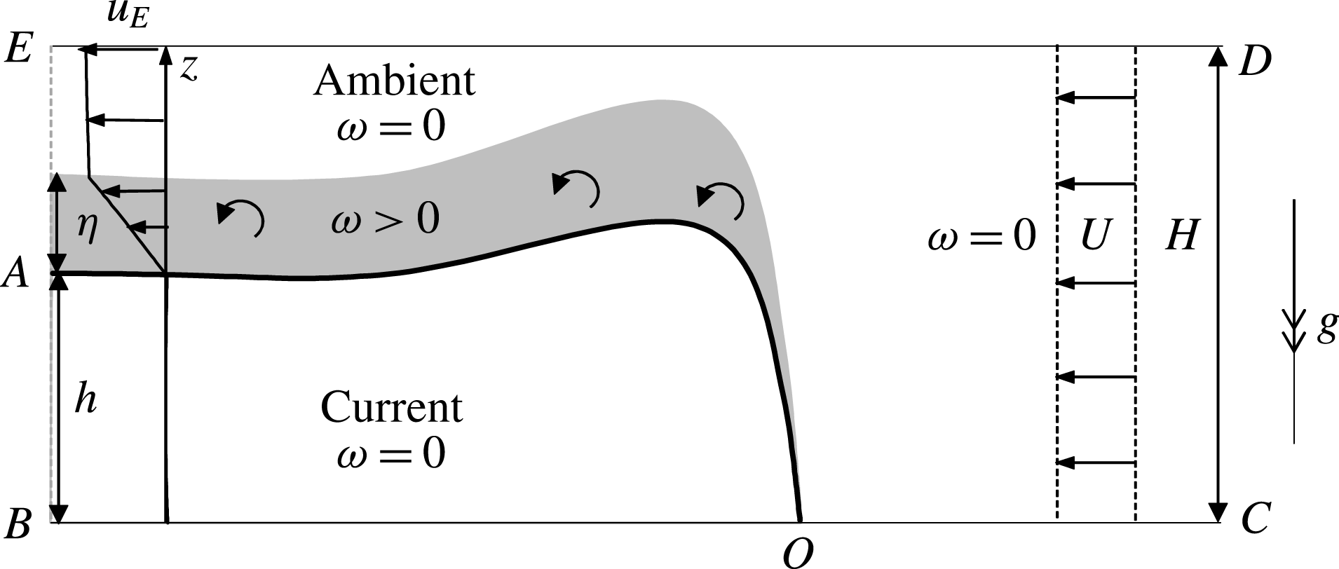
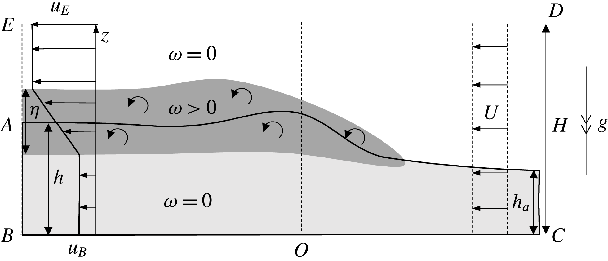
Schematic of the vortex-wake model for flow around the front of a gravity current. Vorticity is only non-vanishing within the layer of thickness
 $\unicode[STIX]{x1D702}$
where the velocity transitions from
 $u=0$
to
 $u=u_{E}$
. Outside this transition layer the vorticity vanishes, and thus there is no head loss on the boundaries
 $BC$
and
 $DE$
(and so
 $\unicode[STIX]{x1D6FF}_{t}=\unicode[STIX]{x1D6FF}_{b}=0$
).

3.2 Vortex-wake model
Our new approach is to close the integral model of mass and momentum balances using the conditions
 $\unicode[STIX]{x1D6FF}_{t}=\unicode[STIX]{x1D6FF}_{b}=0$
on the top and bottom boundaries, but to allow the vortex layer to have non-vanishing thickness (see figure 3). This is in accord with our expectation that the ambient flow is mostly irrotational, therefore
 $\unicode[STIX]{x2202}\unicode[STIX]{x1D714}/\unicode[STIX]{x2202}z=0$
on and near the
 $z=0,H$
boundaries, and, according to (2.18)–(2.19),
 $\unicode[STIX]{x1D6FF}_{t}=\unicode[STIX]{x1D6FF}_{b}=0$
. On the other hand, the viscous and rotational effects exist in a layer close to the interface, and this justifies the finite thickness of the transition region in the velocity field (i.e. there is a vortex layer of thickness
 $\unicode[STIX]{x1D702}$
instead of the vortex sheet as assumed in the classical models).
The governing equations are (3.2)–(3.5) with
 $\unicode[STIX]{x1D6FF}_{t}=\unicode[STIX]{x1D6FF}_{b}=0$
, and the dissipation is given by (3.6). We immediately deduce from (3.3) that
 $Fr\;u_{E}=\sqrt{2}$
and then from (3.4) and (3.5) that
 $$\begin{eqnarray}\displaystyle & \displaystyle Fr^{2}=2\left(1-\int _{0}^{1}f\;\text{d}z\right)^{2}, & \displaystyle\end{eqnarray}$$
 $$\begin{eqnarray}\displaystyle & \displaystyle Fr^{2}=\frac{h\left(1-\displaystyle \int _{0}^{1}f\;\text{d}z\right)^{2}}{2\displaystyle \int _{0}^{1}f\;\text{d}z+\left(\displaystyle \int _{0}^{1}f\;\text{d}z\right)^{2}-2\displaystyle \int _{0}^{1}f^{2}\;\text{d}z}. & \displaystyle\end{eqnarray}$$
We substitute for
 $f(z)$
from (3.2) and eliminate
 $Fr^{2}$
to find that the thickness
 $\unicode[STIX]{x1D702}$
satisfies the following quadratic equation:
 $$\begin{eqnarray}\unicode[STIX]{x1D702}^{2}\left(\int _{0}^{1}\unicode[STIX]{x1D719}(s)\;\text{d}s\right)^{2}+2\unicode[STIX]{x1D702}\left((1+h)\int _{0}^{1}\unicode[STIX]{x1D719}(s)\;\text{d}s-\int _{0}^{1}\unicode[STIX]{x1D719}(s)^{2}\;\text{d}s\right)+\frac{h(2h-1)}{2}=0.\end{eqnarray}$$
It is noteworthy that this quadratic has real roots for
 $0\leqslant h\leqslant 1/2$
, which is the domain of validity. Also from (3.6), the dimensionless dissipation is given by
 $$\begin{eqnarray}\dot{{\mathcal{D}}}=\frac{\sqrt{2}\unicode[STIX]{x1D702}}{h}\int _{0}^{1}(2\unicode[STIX]{x1D719}-\unicode[STIX]{x1D719}^{2})(1-\unicode[STIX]{x1D719})\;\text{d}s.\end{eqnarray}$$
If we now impose a linear variation of the velocity field within the wake
 $\unicode[STIX]{x1D719}(s)=1-s$
, we find the wake thickness, Froude number and dissipation are given by
 $$\begin{eqnarray}\displaystyle \left.\begin{array}{@{}c@{}}\displaystyle \unicode[STIX]{x1D702}=\unicode[STIX]{x1D702}_{L}\equiv \frac{2}{3}\left(\sqrt{1+\frac{21}{2}h}-1-3h\right),\quad Fr=Fr_{L}\equiv \frac{\sqrt{2}}{3}\left(4-\sqrt{1+\frac{21}{2}h}\right)\\ \quad \text{and}\quad \displaystyle \dot{{\mathcal{D}}}=\dot{{\mathcal{D}}}_{L}\equiv {\displaystyle \frac{\sqrt{2}\unicode[STIX]{x1D702}_{L}}{4h}},\end{array}\right\}\quad & & \displaystyle\end{eqnarray}$$
where the subscript
 $L$
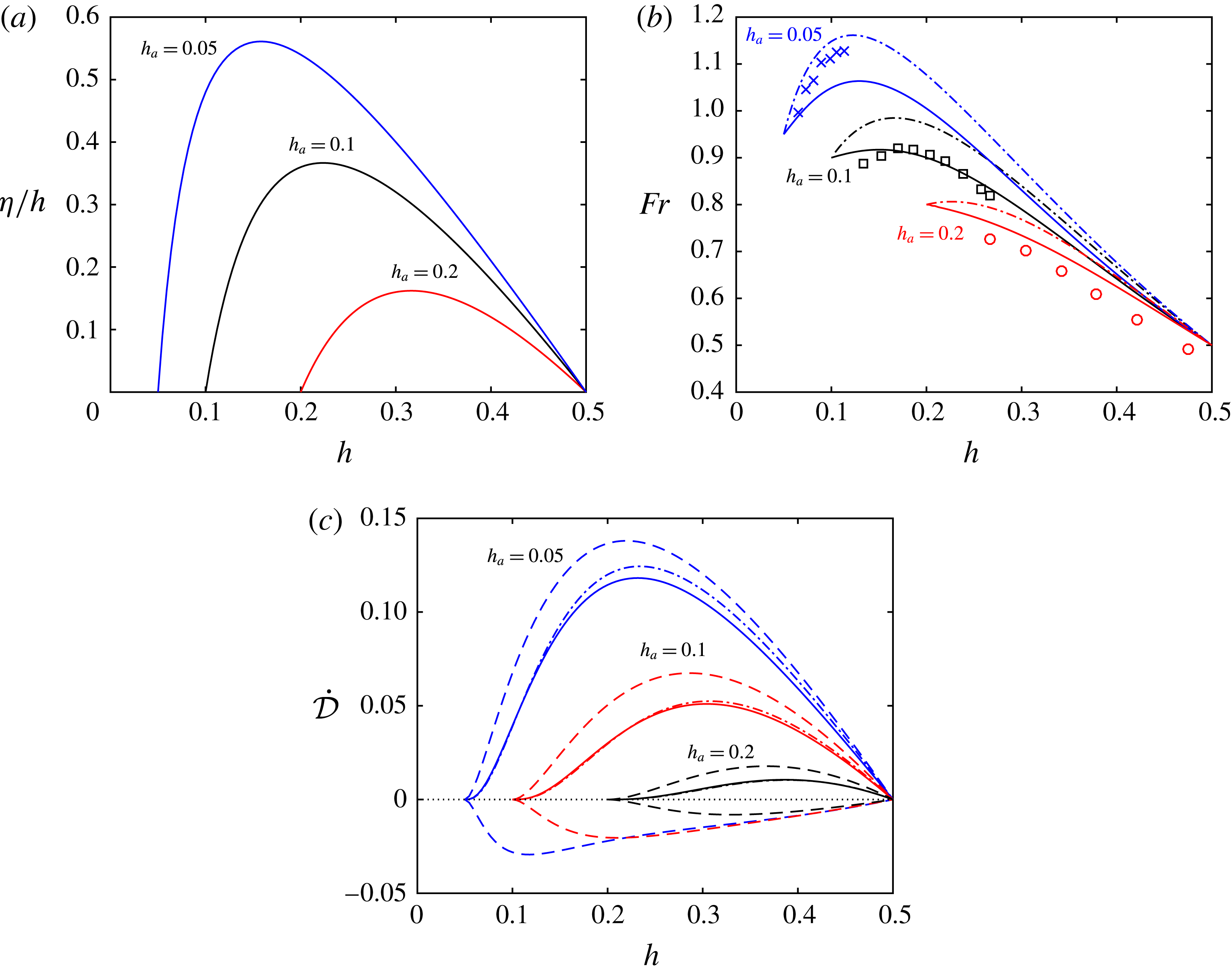
refers to assumption of a linear variation within the wake. These dependencies are plotted in figures 4–6, where we observe that dissipation vanishes when
 $h=1/2$
and reaches a maximum when
 $h\rightarrow 0$
. Notably, when
 $h\ll 1$
we find that
 $$\begin{eqnarray}\unicode[STIX]{x1D702}_{L}=\frac{3h}{2}+\cdots \,,\quad Fr_{L}=\sqrt{2}+\cdots \quad \text{and}\quad \dot{{\mathcal{D}}}_{L}=\frac{3\sqrt{2}}{8}+\cdots \,.\end{eqnarray}$$
Furthermore, when
 $|1/2-h|\ll 1$
we find that
 $$\begin{eqnarray}\unicode[STIX]{x1D702}_{L}=\frac{3}{5}\left(\frac{1}{2}-h\right)+\cdots \,,\quad Fr_{L}=\frac{\sqrt{2}}{2}+\cdots \quad \text{and}\quad \dot{{\mathcal{D}}}_{L}=\frac{3}{5}\left(\frac{1}{2}-h\right)+\cdots \,.\end{eqnarray}$$
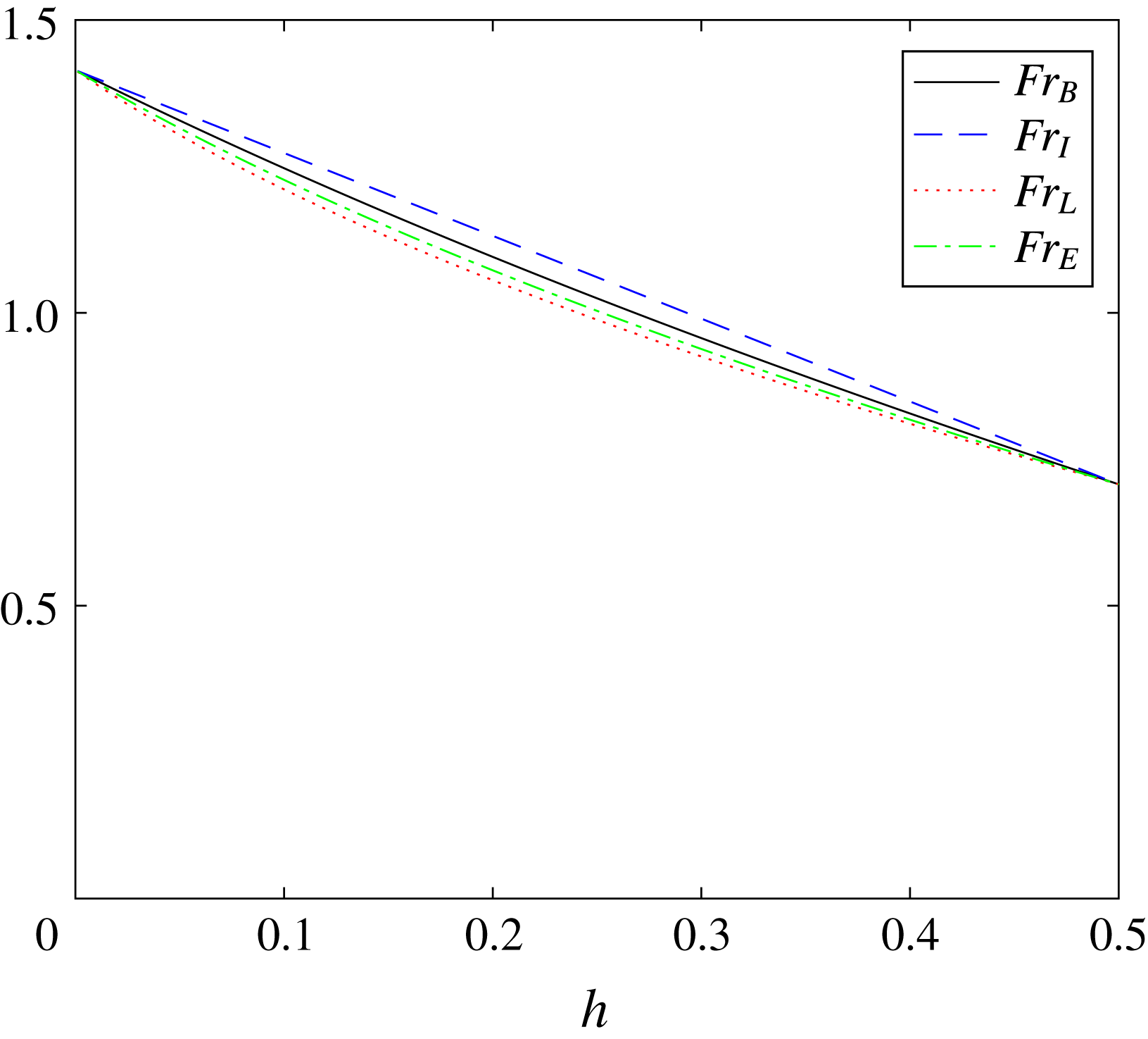
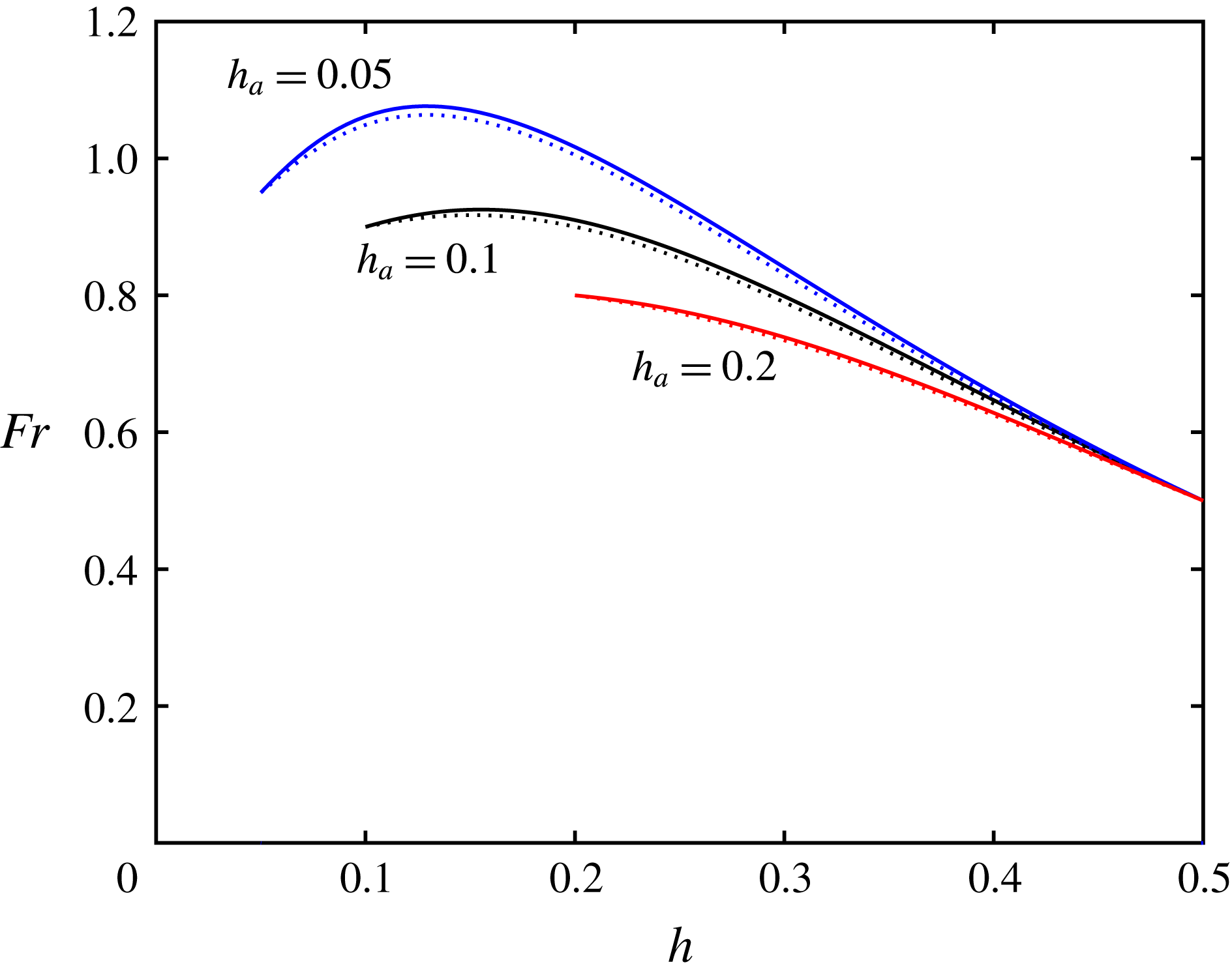
The Froude number,
 $Fr$
, as a function of dimensionless gravity current depth,
 $h$
, for various models: Benjamin,
 $Fr_{B}$
; circulation,
 $Fr_{C}$
; vortex-wake linear,
 $Fr_{L}$
; vortex-wake exponential,
 $Fr_{E}$
.

Conversely if the velocity variation is exponential with
 $\unicode[STIX]{x1D719}(s)=\exp (-\unicode[STIX]{x1D6FC}s)$
, then using
 $\exp (-1/\unicode[STIX]{x1D702})\ll 1$
, the wake thickness and Froude number are given by
 $$\begin{eqnarray}\displaystyle \left.\begin{array}{@{}c@{}}\displaystyle \unicode[STIX]{x1D702}=\unicode[STIX]{x1D702}_{E}\equiv \frac{\unicode[STIX]{x1D6FC}}{2}\left(\sqrt{1+6h}-1-2h\right),\quad Fr=Fr_{E}\equiv \frac{1}{\sqrt{2}}\left(3-\sqrt{1+6h}\right)\\ \quad \text{and}\quad \dot{{\mathcal{D}}}=\dot{{\mathcal{D}}}_{E}\equiv {\displaystyle \frac{5\sqrt{2}\unicode[STIX]{x1D702}_{E}}{6\unicode[STIX]{x1D6FC}h}},\end{array}\right\} & & \displaystyle\end{eqnarray}$$
where the subscript
 $E$
refers to the exponentially varying velocity. It is interesting to note that neither the Froude number,
 $Fr_{E}$
, nor the dissipation
 $\dot{{\mathcal{D}}}_{E}$
depend upon the value of
 $\unicode[STIX]{x1D6FC}$
. Furthermore, if we choose
 $\unicode[STIX]{x1D6FC}=3$
, which corresponds to the velocity field being within 5 % of its asymptotic value at
 $z=h+\unicode[STIX]{x1D702}$
, then
 $\unicode[STIX]{x1D702}_{L}=\unicode[STIX]{x1D702}_{E}=3h/2+\cdots \,$
when
 $h\ll 1$
.
The dissipation,
 $\dot{{\mathcal{D}}}$
, as a function of dimensionless gravity current depth,
 $h$
, for various models: Benjamin,
 $\dot{{\mathcal{D}}}_{B}$
; circulation,
 $\dot{{\mathcal{D}}}_{C}$
; vortex-wake linear,
 $\dot{{\mathcal{D}}}_{L}$
; vortex-wake exponential,
 $\dot{{\mathcal{D}}}_{E}$
.

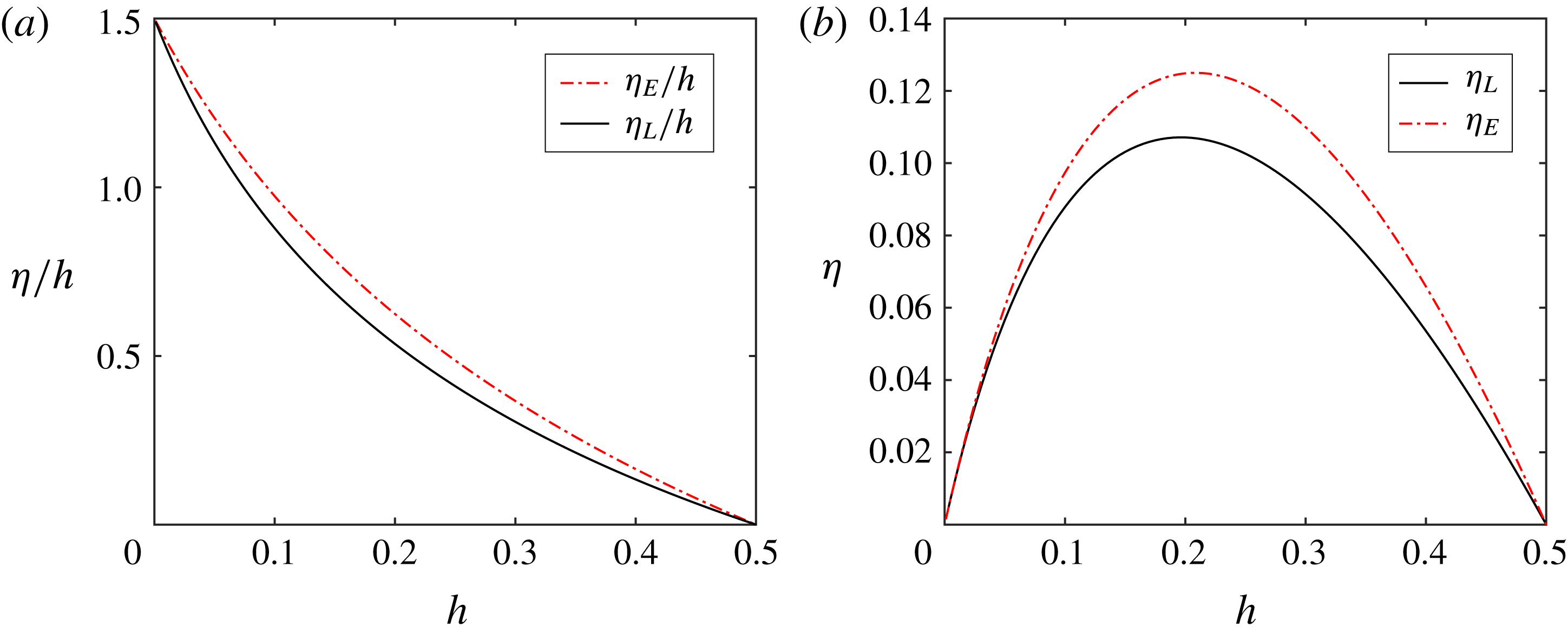
The thickness of the vortex layer,
 $\unicode[STIX]{x1D702}$
, and the relative thickness of the layer,
 $\unicode[STIX]{x1D702}/h$
, as functions of the dimensionless depth of the gravity current for the linear,
 $\unicode[STIX]{x1D702}_{L}$
, and exponential (with
 $\unicode[STIX]{x1D6FC}=3$
),
 $\unicode[STIX]{x1D702}_{E}$
, models of the vortex wake.

Both of these dependencies are plotted in figures 4–6. We note that the predicted Froude numbers from these vortex-wake formulations are very close to those derived by Benjamin (Reference Benjamin1968) and Borden & Meiburg (Reference Borden and Meiburg2013a
) – and the vortex-wake predictions precisely coincide with the inviscid result (3.11) (and with the vortex-sheet models) when
 $h=0$
and
 $h=1/2$
, The largest discrepancy with the Benjamin result is
 $4\,\%$
for the linear profile, and only
 $2\,\%$
for the exponential profile. This is a remarkable agreement. The discrepancies with the circulation-based model of Borden & Meiburg (Reference Borden and Meiburg2013a
) are a little larger (see figure 4).
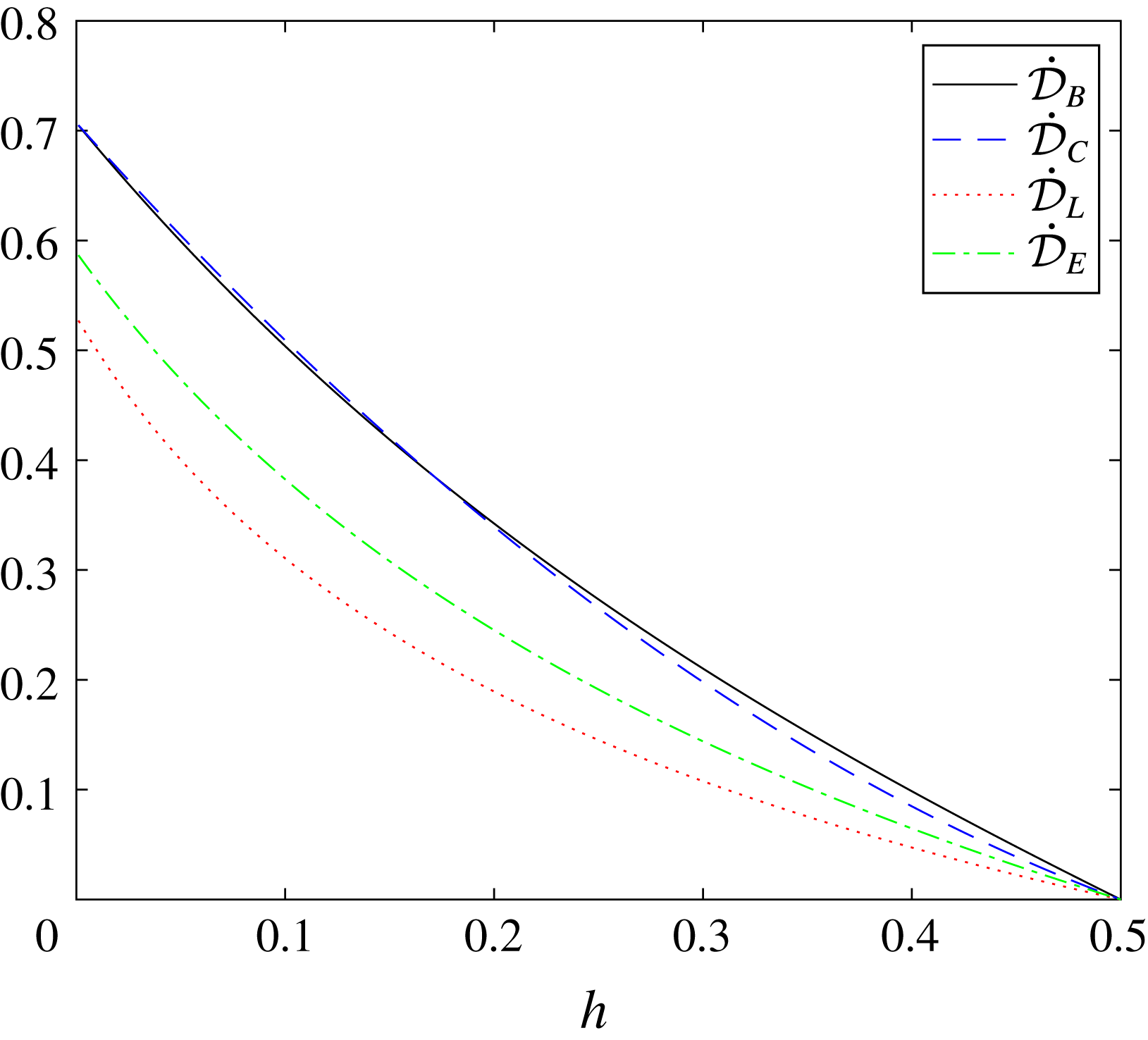
The rate of dissipation is shown in figure 5. Both the classical (
 $\unicode[STIX]{x1D702}=0$
) and vortex-wake (
 $\unicode[STIX]{x1D6FF}_{b}=\unicode[STIX]{x1D6FF}_{t}=0$
) models yield the same qualitative behaviour: a positive dissipation
 $\dot{{\mathcal{D}}}$
which vanishes when
 $h=1/2$
and which is maximised when
 $h=0$
. Quantitatively, the new model is slightly less dissipative. The wake model of Klemp et al. (Reference Klemp, Rotunno and Skamarock1994) led to broadly similar results. However their approach did not explicitly calculate the thickness of the wake,
 $\unicode[STIX]{x1D702}$
, and was based upon a linearisation that neglected the term of order
 $\unicode[STIX]{x1D702}\unicode[STIX]{x1D719}^{2}$
. We note that had this approximation been made in (3.16)–(3.18), then we would have recovered their result for the Froude number,
 $Fr$
.
In figure 6 we show the thickness of the velocity-transition layer for both the linear and exponential variations ((3.20) and (3.23), respectively), where for the latter we choose
 $\unicode[STIX]{x1D6FC}=3$
, so that
 $\unicode[STIX]{x1D719}(1)<0.05$
(i.e. the layer thickness corresponds to the position where the velocity field is within 5 % of its asymptotic value). The interesting feature is that
 $\unicode[STIX]{x1D702}/h$
is finite and non-zero for relatively thin currents
 $h\ll 1$
; the wakes are also relatively thick in this regime. Additionally, the wake thickness vanishes for
 $h=1/2$
and at this value
 $Fr=Fr_{I}=1/\sqrt{2}$
.
3.3 Discussion
The vortex-sheet and vortex-wake models are consistent: their range of validity is
 $0<h\leqslant 1/2$
, the jump is dissipative, and
 $Fr(h)$
is numerically very close to Benjamin’s formula. The vortex-wake model is arguably physically superior to the classical models. The choice of vanishing dissipation along the channel boundaries (
 $BC$
and
 $DE$
) and a finite wake thickness
 $(\unicode[STIX]{x1D6FF}_{t}=\unicode[STIX]{x1D6FF}_{b}=0,\unicode[STIX]{x1D702}>0)$
is more acceptable than
 $\unicode[STIX]{x1D702}=\unicode[STIX]{x1D6FF}_{b}=0,\unicode[STIX]{x1D6FF}_{t}>0$
. While a finite (even thick) velocity-transition layer makes sense, the concept that sufficient vorticity is present near the upper boundary of the channel to provide a non-vanishing vorticity flux (and a non-vanishing
 $\unicode[STIX]{x1D6FF}_{t}$
) is rather artificial. The classical expression due to Benjamin (Reference Benjamin1968) yields
 $Fr_{B}(h)$
as a simple unique formula, while the vortex-wake model prediction for
 $Fr$
depends (slightly) on the assumed profile of velocity through transition layer. However, the former is based upon the assumption of a discontinuous change in the velocity. Instead the vortex-wake model introduces the physically consistent, continuous adjustment of the velocity field and thus its predictions for the Froude number,
 $Fr_{E}$
(and
 $Fr_{L}$
), are strong competitors to
 $Fr_{B}$
.
4 Internal jump problem
The general configuration for internal jumps is sketched in figure 1(b) in a frame of reference in which the jump is stationary. The important difference from gravity current flow is that the layer of relatively dense fluid extends upstream (so that
 $R=1+S$
) and flows across the segment
 $CD$
with speed
 $U$
. The lower, dense layer expands and decelerates, whereas the upper less dense fluid contracts and accelerates. This motion produces vorticity (
 $\unicode[STIX]{x1D714}>0$
) about the interface and also within the layers. The problem is specified by two dimensionless parameters: the excess density ratio
 $S$
(2.17) and
 $h_{a}$
, which measures the upstream depth of dense fluid relative to the channel depth.
We use balances of mass and streamwise momentum within a control volume
 $ABCDE$
(see figure 1
b), together with the expression of consistency to ensure a single-valued pressure field (which is shown to be equivalent to the balance of vorticity in appendix A), to model the motion. The dimensionless governing equations are given by (2.20)–(2.23), and we examine their form when there is negligible mixing of solute between the layers so that
 $r(z)$
is piecewise constant and the velocity field
 $$\begin{eqnarray}u(z)=(u_{B}+u_{E})/2+(u_{E}-u_{B})f(z)/2\end{eqnarray}$$
takes the following form:
 $$\begin{eqnarray}r(z)=\left\{\begin{array}{@{}ll@{}}1,\quad & 0\leqslant z\leqslant h\\ 0,\quad & h\leqslant z\leqslant 1\end{array}\right.\quad \text{and}\quad f(z)=\unicode[STIX]{x1D713}\left(\frac{(z-h)}{\unicode[STIX]{x1D702}}\right),\end{eqnarray}$$
where
 $\unicode[STIX]{x1D702}$
is the thickness of the layer over which the velocity field transitions from
 $u_{B}$
to
 $u_{E}$
. The function
 $\unicode[STIX]{x1D713}$
satisfies
 $\unicode[STIX]{x1D713}(0)=0$
and
 $\unicode[STIX]{x1D713}(s)=s/|s|$
for
 $|s|\geqslant 1$
.
Conservation of mass (2.20) then gives
 $$\begin{eqnarray}\frac{1}{2}(u_{B}+u_{E})+\frac{1}{2}(u_{E}-u_{B})\int _{0}^{1}f\;\text{d}z=1,\end{eqnarray}$$
and conservation of solute (2.21) yields
 $$\begin{eqnarray}\frac{1}{2}(u_{B}+u_{E})h+\frac{1}{2}(u_{E}-u_{B})\int _{0}^{h}f\;\text{d}z=h_{a}.\end{eqnarray}$$
The dimensionless condition for the consistency of the pressure field (2.22) gives
 $$\begin{eqnarray}\frac{Fr^{2}}{2}(u_{E}^{2}-(1+S)u_{B}^{2}+S)=1-\frac{h_{a}}{h}-\unicode[STIX]{x1D6FF}_{t}+\unicode[STIX]{x1D6FF}_{b}.\end{eqnarray}$$
Finally the dimensionless balance of streamwise momentum (2.23) is expressed by
 $$\begin{eqnarray}Fr^{2}\left(\frac{u_{E}^{2}}{2}-\int _{0}^{1}u^{2}\;\text{d}z-S\int _{0}^{h}u^{2}\;\text{d}z+\frac{1}{2}+Sh_{a}\right)+\unicode[STIX]{x1D6FF}_{t}=\frac{h^{2}-h_{a}^{2}}{2h}.\end{eqnarray}$$
In the inviscid limit
 $(\unicode[STIX]{x1D6FF}_{t}=\unicode[STIX]{x1D6FF}_{b}=\unicode[STIX]{x1D702}=0)$
, (4.5) and (4.6) provide expressions for the speed of the jump in terms of
 $h_{a}$
and
 $S$
. For instance from (4.5) we find that
 $$\begin{eqnarray}\displaystyle Fr^{2}=Fr_{I}^{2} & \equiv & \displaystyle \frac{2(h-h_{a})}{h}\left(\frac{(1-h_{a})^{2}}{(1-h)^{2}}-(1+S)\frac{h_{a}^{2}}{h^{2}}+S\right)^{-1}\nonumber\\ \displaystyle & = & \displaystyle \frac{2h(1-h)^{2}}{S(1-h)^{2}(h+h_{a})-2h_{a}h+h_{a}+h}.\end{eqnarray}$$
However, by substituting this result in (4.6), we find that this inviscid result is only valid when
 $h=h_{a}$
(which is a trivial result as there is no jump), and
 $$\begin{eqnarray}h=\frac{1+S-\sqrt{1+S}}{S}.\end{eqnarray}$$
Note that in the Boussinesq regime
 $(S\ll 1)$
,
 $h=1/2+\cdots \,$
, which recovers the same condition as for gravity currents. We encounter again the issue that at least one of
 $\unicode[STIX]{x1D6FF}_{t}$
,
 $\unicode[STIX]{x1D6FF}_{b}$
and
 $\unicode[STIX]{x1D702}$
must be non-vanishing for a more general solution.
We now specialise to two important classes of solution, namely the vortex sheet (§ 4.1), for which the velocity field changes discontinuously
 $(\unicode[STIX]{x1D702}=0)$
, and the vortex wake (§ 4.2), in which the velocity field transitions over some finite, non-vanishing extent.
4.1 Vortex-sheet model
$(\unicode[STIX]{x1D702}=0)$

In a vortex-sheet model of the flow downstream from the internal jump, both the density and velocity fields are discontinuous at the interface
 $z=h$
, and in terms of the expression for the velocity field given in (4.2), we impose
 $\unicode[STIX]{x1D713}(s)=s/|s|$
. Then from (4.3) and (4.4) we deduce
 $$\begin{eqnarray}u_{B}=\frac{h_{a}}{h}\quad \text{and}\quad u_{E}=\frac{1-h_{a}}{1-h}.\end{eqnarray}$$
Substituting these expressions into (4.5) and (4.6) we find two coupled algebraic equations for three variables,
 $Fr$
,
 $\unicode[STIX]{x1D6FF}_{t}$
and
 $\unicode[STIX]{x1D6FF}_{b}$
, given by
 $$\begin{eqnarray}\displaystyle & \displaystyle \frac{Fr^{2}}{2}\left(\left(\frac{1-h_{a}}{1-h}\right)^{2}-(1+S)\frac{h_{a}^{2}}{h^{2}}+S\right)=1-\frac{h_{a}}{h}+\unicode[STIX]{x1D6FF}_{b}-\unicode[STIX]{x1D6FF}_{t}, & \displaystyle\end{eqnarray}$$
 $$\begin{eqnarray}\displaystyle & \displaystyle Fr^{2}\left(\frac{1}{2}\left(\frac{1-h_{a}}{1-h}\right)^{2}-\frac{(1-h_{a})^{2}}{(1-h)}-(1+S)\frac{h_{a}^{2}}{h}+\frac{1}{2}+Sh_{a}\right)+\unicode[STIX]{x1D6FF}_{t}=\frac{h^{2}-h_{a}^{2}}{2h}. & \displaystyle\end{eqnarray}$$
Since the velocity field on the outflow is piecewise constant, a Bernoulli balance yields that head loss on each streamline in the upper fluid is
 $\unicode[STIX]{x1D6FF}_{t}$
, while it is
 $\unicode[STIX]{x1D6FF}_{b}$
in the lower fluid. We may thus evaluate the dimensionless dissipation in the flow, which can be rewritten as
 $$\begin{eqnarray}\dot{{\mathcal{D}}}=\frac{Fr}{h}(\unicode[STIX]{x1D6FF}_{t}(1-h_{a})+\unicode[STIX]{x1D6FF}_{b}h_{a}).\end{eqnarray}$$
We may readily identify this expression for the dissipation as the sum from each layer. Physical considerations demand that the total dissipation must be positive semi-definite
 $\dot{{\mathcal{D}}}\geqslant 0$
, but importantly this criterion does not imply that both layers must be dissipative.
To complete the model, we must invoke a closure assumption because our systems is reduced to three variables
 $(Fr,\unicode[STIX]{x1D6FF}_{t},\unicode[STIX]{x1D6FF}_{b})$
and two equations (4.10) and (4.11). This situation is entirely analogous to the problem for gravity current fronts – and in the context of internal jumps, different investigators have adopted different strategies (see Wood & Simpson Reference Wood and Simpson1984; Klemp et al.
Reference Klemp, Rotunno and Skamarock1997; Li & Cummins Reference Li and Cummins1998; Borden & Meiburg Reference Borden and Meiburg2013b
; Baines Reference Baines2016). We find that it is convenient to write
 $\unicode[STIX]{x1D6FF}_{b}=\unicode[STIX]{x1D706}\unicode[STIX]{x1D6FF}_{t}$
and then eliminating
 $\unicode[STIX]{x1D6FF}_{t}$
between (4.10) and (4.11), we find that
 $$\begin{eqnarray}Fr^{2}=\frac{(h-h_{a})(1+\textstyle \frac{1}{2}(\unicode[STIX]{x1D706}-1)(h+h_{a}))}{h(q_{1}+(\unicode[STIX]{x1D706}-1)q_{2})},\end{eqnarray}$$
where
 $$\begin{eqnarray}\displaystyle & \displaystyle q_{1}=\frac{1}{2}\left(\frac{(1-h_{a})^{2}}{(1-h)^{2}}-(1+S)\frac{h_{a}^{2}}{h^{2}}+S\right), & \displaystyle\end{eqnarray}$$
 $$\begin{eqnarray}\displaystyle & \displaystyle q_{2}=\frac{1}{2}\frac{(1-h_{a})^{2}}{(1-h)^{2}}-\frac{(1-h_{a})^{2}}{1-h}-(1+S)\frac{h_{a}^{2}}{h}+\frac{1}{2}+Sh_{a}. & \displaystyle\end{eqnarray}$$
We may then recover different formulae by substituting different values of
 $\unicode[STIX]{x1D706}$
(cf. Li & Cummins Reference Li and Cummins1998). Wood & Simpson (Reference Wood and Simpson1984) assumed that there was no dissipation in the contracting layer and so
 $\unicode[STIX]{x1D6FF}_{t}=0$
(
 $\unicode[STIX]{x1D706}\rightarrow \infty$
). In contrast Klemp et al. (Reference Klemp, Rotunno and Skamarock1997) assumed that there was no dissipation in the expanding layer, expressed as
 $\unicode[STIX]{x1D6FF}_{b}=0$
and so
 $\unicode[STIX]{x1D706}=0$
. Finally, and most recently, Borden & Meiburg (Reference Borden and Meiburg2013b
) and Baines (Reference Baines2016) assumed a form of vorticity conservation that is equivalent to assuming that the dissipation per unit mass along the bounding streamlines
 $DE$
and
 $BC$
is equal (
 $\unicode[STIX]{x1D6FF}_{b}=(1+S)\unicode[STIX]{x1D6FF}_{t}$
). We also note that that if
 $\unicode[STIX]{x1D706}=1$
then the deduced Froude number from (4.13) is equal to the ideal, ‘inviscid’ result (4.7), although the dissipation is not necessarily vanishing in this case. It is evident therefore that all previous expressions for the speed of the bore require, or imply, a closure assumption.
Previous investigations invested considerable effort into the question of which of these many variants is preferable. These studies do not provide a theoretical criterion for the choice of
 $\unicode[STIX]{x1D706}$
, and actually there is no reason why
 $\unicode[STIX]{x1D706}$
should be a constant. The main comparison has been between measurement of the speed of the jump,
 $U$
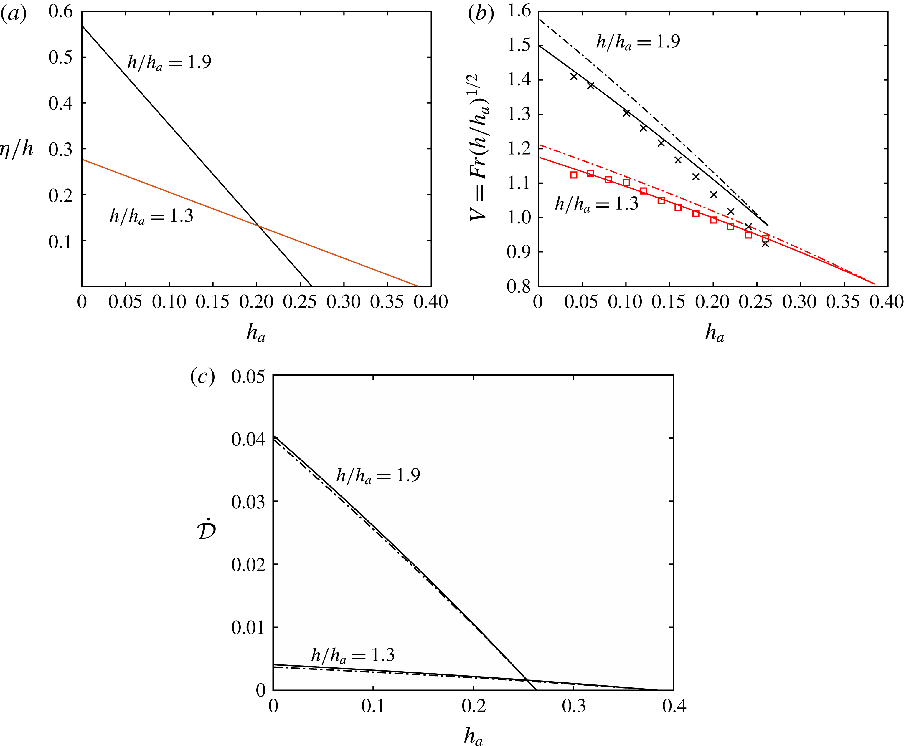
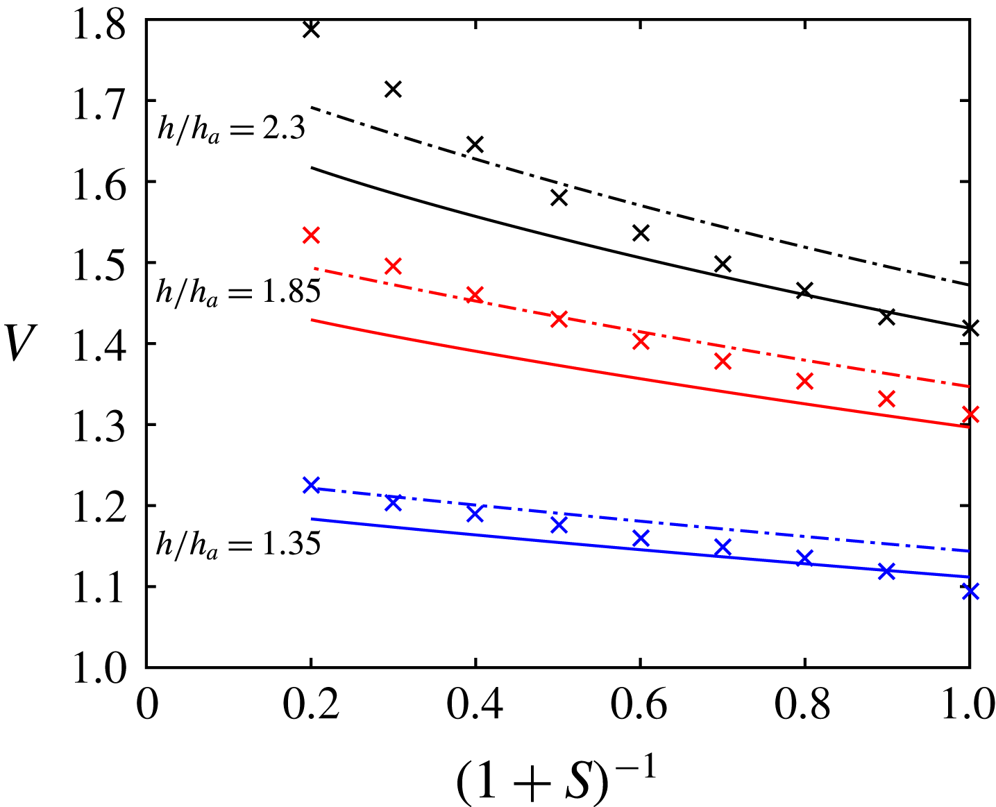
, in laboratory experiments and Navier–Stokes simulations, and the model predictions, along with qualitative arguments concerning the dissipation. In general, the conclusion is that the model due to Klemp et al. (Reference Klemp, Rotunno and Skamarock1997) performs better than that of Wood & Simpson (Reference Wood and Simpson1984) (although the predicted
 $U$
often exceeds the data). The circulation-based models of
 $U$
are close to, but slightly larger than, the Klemp et al. (Reference Klemp, Rotunno and Skamarock1997) results. However there are difficulties in drawing firm conclusions from comparisons with laboratory experiments and simulation data, because they are usually restricted to a relatively narrow range of flow parameters (e.g. the flows are often Boussinesq and with equal viscosities). The assumptions of the modelled flow (e.g. free-slip boundaries, laminar steady state, Schmidt number
 $Sc\rightarrow \infty$
) do not conform precisely to either laboratory experiments or computational simulations. Moreover, there is no theoretical interpretation or criterion to underpin the modelling and closure assumptions.
Schematic of the vorticity,
 $\unicode[STIX]{x1D714}$
, distribution in a two-layer jump under the classical model of a vortex sheet at
 $A$
. The vorticity vanishes (
 $\unicode[STIX]{x1D714}=0$
) at the boundaries of the control volume, except for at the vortex sheet. The eddies indicate vorticity generation and note that
 $\unicode[STIX]{x1D714}>0$
in the lower (expanding) layer. This implies that
 $\unicode[STIX]{x2202}\unicode[STIX]{x1D714}/\unicode[STIX]{x2202}z>0$
, and
 $\unicode[STIX]{x1D6FF}_{b}<0$
. This scenario demonstrates that under the ‘classical’ model of a vortex sheet that it is inconsistent to set
 $\unicode[STIX]{x1D6FF}_{b}=(1+S)\unicode[STIX]{x1D6FF}_{t}$
since they must be opposite signed and furthermore because the total dissipation must be positive, there must be dissipation in the upper contracting layer (thus supporting the model of Klemp et al. (Reference Klemp, Rotunno and Skamarock1997)).

We suggest a more self-contained approach. We exploit again the connection between the boundary head losses,
 $\unicode[STIX]{x1D6FF}_{t}$
and
 $\unicode[STIX]{x1D6FF}_{b}$
, and the boundary gradients of vorticity,
 $\unicode[STIX]{x2202}\unicode[STIX]{x1D714}/\unicode[STIX]{x2202}z$
(see (2.18) and (2.19)). The expected vorticity distribution is shown in figure 7. The lower layer expands, the upper contracts, and hence
 $u_{2}>u_{1}$
and
 $\unicode[STIX]{x1D714}>0$
is produced at the interface. In view of the
 $\unicode[STIX]{x1D714}=0$
boundary conditions at
 $z=0$
and
 $1$
,
 $(\unicode[STIX]{x2202}\unicode[STIX]{x1D714}/\unicode[STIX]{x2202}z)>0$
in the region with fluid of density
 $\unicode[STIX]{x1D70C}_{1}$
and
 $(\unicode[STIX]{x2202}\unicode[STIX]{x1D714}/\unicode[STIX]{x2202}z)<0$
in the region with fluid of density
 $\unicode[STIX]{x1D70C}_{2}$
. Thus according to (2.18)–(2.19), we deduce that
 $\unicode[STIX]{x1D6FF}_{t}>0$
and
 $\unicode[STIX]{x1D6FF}_{b}<0$
. In other words, the upper layer is dissipative, while the lower one gains energy: see (4.12). Immediately this implies that the model due to Wood & Simpson (Reference Wood and Simpson1984) is problematic: by imposing
 $\unicode[STIX]{x1D6FF}_{t}=0$
and
 $\unicode[STIX]{x1D6FF}_{b}>0$
, it prevents the dissipation effect from the proper layer, and enforces it on the wrong layer. The model due to Klemp et al. (Reference Klemp, Rotunno and Skamarock1997) with
 $\unicode[STIX]{x1D6FF}_{t}>0$
and
 $\unicode[STIX]{x1D6FF}_{b}=0$
, on the other hand, is consistent with the vorticity field in the upper (major) layer, while the needed negative
 $\unicode[STIX]{x1D6FF}_{b}$
is approximated by assuming that it vanishes. The circulation-based model with
 $\unicode[STIX]{x1D6FF}_{t}>0,\unicode[STIX]{x1D6FF}_{b}>0$
is consistent with the vorticity field in the upper layer, but imposes the wrong sign in the lower layer. On balance, therefore, the model due to Klemp et al. (Reference Klemp, Rotunno and Skamarock1997) appears to be the most consistent compromise. We emphasise that we used no arguments concerning the energetics of the flow in our assessment of the models with different
 $\unicode[STIX]{x1D6FF}_{t}$
and
 $\unicode[STIX]{x1D6FF}_{b}$
, in contrast with the widely accepted suggestion of Li & Cummins (Reference Li and Cummins1998).
The expressions of head loss on streamlines (2.18)–(2.19) reveal that
 $\unicode[STIX]{x1D6FF}_{t}$
and
 $\unicode[STIX]{x1D6FF}_{b}$
can be interpreted as distributed viscous drag forces per unit area, which arise due to shear at the interface downstream of the internal jump. The contracting upper layer moves faster than the expanding lower layer, and hence a positive drag is expected in this domain,
 $\unicode[STIX]{x1D6FF}_{t}>0$
. By the same argument,
 $\unicode[STIX]{x1D6FF}_{b}<0$
– and therefore the inferred signs of these terms are in agreement with the argument developed above. Moreover, in vorticity balance (A 2), the term
 $\unicode[STIX]{x1D6FF}_{b}-\unicode[STIX]{x1D6FF}_{t}$
can be interpreted as the torque of the distributed drag forces, and we expect it to be negative (clockwise).
Together, these observations yield a simple guiding principle for the closures for classical (vortex-sheet) models of internal jumps. In general, the head loss in the contracting layer must be positive, and in the expanding layer negative. From (4.10), we see that the head loss terms
 $\unicode[STIX]{x1D6FF}_{t}>0$
and
 $\unicode[STIX]{x1D6FF}_{b}<0$
lead to a reduction in predicted speed of the jump,
 $Fr$
and the inviscid expression,
 $Fr_{I}$
, is the upper bound of this result, as expected. We note again that the situation
 $\unicode[STIX]{x1D6FF}_{b}=\unicode[STIX]{x1D6FF}_{t}$
, which also reproduces
 $Fr_{I}$
, contradicts the observation that
 $\unicode[STIX]{x1D6FF}_{b}>0$
and therefore lacks physical justification.
The validity of the models is traditionally restricted by requiring the total dissipation
 $\dot{{\mathcal{D}}}\geqslant 0$
. We comment that this is not a sharp criterion in general, because some models employ non-physical
 $\unicode[STIX]{x1D6FF}_{b}>0$
, and this distorts the value of
 $\dot{{\mathcal{D}}}$
. This is in particular problematic for the model due to Wood & Simpson (Reference Wood and Simpson1984) and circulation-based models (Borden & Meiburg Reference Borden and Meiburg2013a
; Baines Reference Baines2016). The model due to Klemp et al. (Reference Klemp, Rotunno and Skamarock1997) imposes vanishing dissipation in the lower layer (
 $\unicode[STIX]{x1D6FF}_{b}=0$
and
 $\dot{{\mathcal{D}}_{1}}=0$
) and thus demands that the upper layer alone is dissipative (so that
 $\dot{{\mathcal{D}}}>0$
), whereas the discussion above indicates that
 $\unicode[STIX]{x1D6FF}_{b}<0$
is consistent with the anticipated distribution of vorticity.
We conclude that considerations of the vorticity distribution are sharper than the energy-dissipation arguments (although the latter are still of value). For example, these considerations predict that the model due to Klemp et al. (Reference Klemp, Rotunno and Skamarock1997) is preferable to the other closures – and we know that it is in broad agreement with the data. However, the new insights are still mostly qualitative. We argue with confidence that the ratio
 $\unicode[STIX]{x1D6FF}_{b}/\unicode[STIX]{x1D6FF}_{t}<0$
should be negative and finite. A model with
 $\unicode[STIX]{x1D6FF}_{b}/\unicode[STIX]{x1D6FF}_{t}<0$
will be an improved substitute to the Klemp et al. (Reference Klemp, Rotunno and Skamarock1997) model (
 $\unicode[STIX]{x1D6FF}_{b}=0$
), but we do not have a reliable estimate for the optimal value of this ratio.
4.2 The vortex-wake model
Schematic of the vorticity
 $\unicode[STIX]{x1D714}$
distribution in an internal jump with a finite, non-vanishing thickness transition layer over which the velocity varies from
 $u_{B}$
to
 $u_{E}$
. Vorticity is non-vanishing within this layer, but vanishes everywhere else within the domain.

In this section we examine a different closure, namely the existence of a finite thickness layer through which the velocity varies from
 $u_{B}$
to
 $u_{E}$
(see figure 8). Within this layer there is non-vanishing vorticity generated by the baroclinic torque associated with the expansion of the lower, relatively dense layer. We examine the dynamics integrated over a control volume enclosing the jump on the assumption that streamlines of the motion have become parallel with the channel boundaries at the segment
 $BE$
and the dissipative effects at the boundary vanish, so that
 $\unicode[STIX]{x1D6FF}_{b}=\unicode[STIX]{x1D6FF}_{t}=0$
.
The velocity is assumed to transition between
 $z=h-\unicode[STIX]{x1D702}$
and
 $z=h+\unicode[STIX]{x1D702}$
on the assumption that the viscosities of the two fluids are comparable (and the extension to differing viscosities and the resultant asymmetric velocity fields is tackled below). It will also be assumed, and later confirmed, that
 $\unicode[STIX]{x1D702}<h$
and
 $\unicode[STIX]{x1D702}<1-h$
, so that the transition layer is separate from the channel boundaries. Here we model a linear variation within the layer, so that
 $\unicode[STIX]{x1D713}(s)=s$
for
 $|s|<1$
and
 $\unicode[STIX]{x1D713}(s)=s/|s|$
for
 $|s|>1$
, and in appendix B we analyse an alternative that yields almost identical results.
The flow is modelled using (2.20)–(2.23), for which we need the following integrals:
 $$\begin{eqnarray}\int _{0}^{1}f\;\text{d}z=1-2h,\quad \int _{0}^{h}f\;\text{d}z=-h+\frac{1}{2}\unicode[STIX]{x1D702},\end{eqnarray}$$
 $$\begin{eqnarray}\int _{0}^{1}f^{2}\;\text{d}z=1-\frac{4}{3}\unicode[STIX]{x1D702},\quad \int _{0}^{h}f^{2}\;\text{d}z=h-\frac{2}{3}\unicode[STIX]{x1D702}.\end{eqnarray}$$
Conservation of mass and solute then yields
 $$\begin{eqnarray}u_{E}(1-h)+u_{B}h=1\quad \text{and}\quad u_{B}(h-\textstyle \frac{1}{4}\unicode[STIX]{x1D702})+\textstyle \frac{1}{4}u_{E}\unicode[STIX]{x1D702}=h_{a}.\end{eqnarray}$$
The requirement of a single-valued pressure field given by
 $$\begin{eqnarray}Fr^{2}(u_{E}^{2}-(1+S)u_{B}^{2}+S)=\frac{2(h-h_{a})}{h}.\end{eqnarray}$$
Finally the balance of streamwise momentum leads to
 $$\begin{eqnarray}\displaystyle & & \displaystyle Fr^{2}\left[u_{E}^{2}\left(h-\frac{1}{2}+\frac{\unicode[STIX]{x1D702}}{3}-\frac{S\unicode[STIX]{x1D702}}{12}\right)-u_{B}^{2}\left(h(1+S)-\frac{\unicode[STIX]{x1D702}}{3}-\frac{5S\unicode[STIX]{x1D702}}{12}\right)\right.\nonumber\\ \displaystyle & & \displaystyle \qquad \left.-\,u_{E}u_{B}\left(\frac{2}{3}+\frac{S}{3}\right)\unicode[STIX]{x1D702}+\frac{1}{2}+Sh_{a}\right]=\frac{h^{2}-h_{a}^{2}}{2h}.\end{eqnarray}$$
It is possible to solve these algebraic equations to find that the dimensionless speed of the internal jump, expressed as
 $Fr$
, satisfies
 $$\begin{eqnarray}Fr^{2}=\frac{1}{4h}\frac{[4h(1-h)-\unicode[STIX]{x1D702}]^{2}}{[(Sh-(S+1))\unicode[STIX]{x1D702}+2(S(1-h)^{2}.(h+h_{a})-2hh_{a}+h+h_{a})]}.\end{eqnarray}$$
Note that this expression reduces to the inviscid result
 $Fr=Fr_{I}$
(see (4.7)) when
 $\unicode[STIX]{x1D702}=0$
. The thickness of the transition layer is determined by the quadratic equation
 $$\begin{eqnarray}\displaystyle & & \displaystyle 3S\unicode[STIX]{x1D702}^{2}-2[3Sh(h-3h_{a})+6Sh_{a}+(S+5)(h_{a}-h)]\unicode[STIX]{x1D702}\nonumber\\ \displaystyle & & \displaystyle \quad -\,12(h_{a}-h)^{2}(S(1-h)^{2}-2h+1)=0.\end{eqnarray}$$
It is noteworthy that this expression has real solutions when
 $h_{a}<h<(S+1-\sqrt{1+S})/S$
and that
 $\unicode[STIX]{x1D702}$
vanishes as the largest and smallest values of
 $h$
in this range, yielding the ‘inviscid’ solution for
 $Fr=Fr_{I}$
(4.7). Furthermore, for Boussinesq jumps
 $(S=0)$
, we immediately deduce that
 $$\begin{eqnarray}\unicode[STIX]{x1D702}=\frac{6}{5}(h-h_{a})(1-2h)\quad \text{and}\quad Fr^{2}=\frac{(4h^{2}-7h-3h_{a}(1-2h))^{2}}{20h(3h^{2}+h+4h_{a}(1-2h))}.\end{eqnarray}$$
Dissipation is a by-product of this calculation. By substituting the assumed forms of the velocity we may evaluate the dimensionless dissipation in the lower and upper layers, denoted by
 $\dot{{\mathcal{D}}}_{1}$
and
 $\dot{{\mathcal{D}}}_{2}$
, respectively, and given by
 $$\begin{eqnarray}\dot{{\mathcal{D}}}_{1}=-\frac{Fr^{3}\unicode[STIX]{x1D702}(1+S)}{64h}(u_{E}-u_{B})(u_{E}+3u_{B})^{2}\quad \text{and}\quad \dot{{\mathcal{D}}}_{2}=\frac{Fr^{3}\unicode[STIX]{x1D702}}{64h}(u_{E}-u_{B})(3u_{E}+u_{B})^{2}.\end{eqnarray}$$
Thus we deduce that since
 $u_{B}<u_{E}$
there is in general some energy gain in the lower layer since
 $\dot{{\mathcal{D}}}_{1}<0$
. In the upper layer there is dissipation
 $(\dot{{\mathcal{D}}}_{2}>0)$
and in general for Boussinesq systems for which
 $u_{B}\ll u_{E}$
,
 $\dot{{\mathcal{D}}}_{2}\gg |\dot{{\mathcal{D}}}_{1}|$
. We reiterate that this result is an intrinsic outcome of the vortex-wake solution and furthermore we note that the flow is only non-dissipative when
 $\unicode[STIX]{x1D702}=0$
, which occurs at
 $h=(S+1-\sqrt{1+S})/S$
, in addition to the trivial cases
 $h=h_{a}$
(and
 $u_{B}=u_{E}$
).
Properties of an internal jump as functions of the dimensionless downstream thickness of the jump,
 $h$
, for various dimensionless upstream thicknesses: (a) the scaled thickness of the vortex-wake,
 $\unicode[STIX]{x1D702}/h$
; (b) the Froude number of the jump,
 $Fr$
; (c) the dissipation in each layer,
 $\dot{{\mathcal{D}}}_{1}({<}0)$
and
 $\dot{{\mathcal{D}}}_{2}$
(dashed lines) and the total dissipation
 $\dot{{\mathcal{D}}}_{1}+\dot{{\mathcal{D}}}_{2}$
(solid lines). In (b) and (c), the prediction from the vortex-sheet model due to Klemp et al. (Reference Klemp, Rotunno and Skamarock1994) are also plotted (dot-dash lines). In (b) the data points are from the simulations reported by Borden et al. (Reference Borden, Meiburg and Constantinescu2012b
) for
 $h_{a}=0.2$
 $(\circ )$
,
 $h_{a}=0.1$
(▫) and
 $h_{a}=0.05~(\times )$
.

Properties of an internal jump as functions of the dimensionless downstream thickness of the jump,
 $h$
, for various dimensionless upstream thicknesses: (a) the scaled thickness of the vortex-wake,
 $\unicode[STIX]{x1D702}/h$
; (b) the dimensionless speed of the jump,
 $V$
; (c) the total dissipation
 $\dot{{\mathcal{D}}}$
(solid lines). In (b) and (c), the prediction from the vortex-sheet model due to Klemp et al. (Reference Klemp, Rotunno and Skamarock1994) is also plotted (dot-dash lines). In (b) the data points are from the simulations reported by Borden et al. (Reference Borden, Meiburg and Constantinescu2012b
) for
 $h/h_{a}=1.3~(\times )$
and
 $h/h_{a}=1.3$
(▫).

We illustrate our results in figures 9 and 10 for the Boussinesq regime
 $(S=0)$
. In figure 9, we plot the scaled thickness,
 $\unicode[STIX]{x1D702}/h$
, the Froude number of the jump,
 $Fr$
, and dissipation,
 $\dot{{\mathcal{D}}}_{1}$
and
 $\dot{{\mathcal{D}}}_{2}$
, as functions of the dimensionless downstream thickness of the jump,
 $h$
, along with the predictions from the vortex-sheet model due to Klemp et al. (Reference Klemp, Rotunno and Skamarock1997) (for which
 $\unicode[STIX]{x1D706}=0$
in (4.13)) and with results from Navier–Stokes simulations due to Borden et al. (Reference Borden, Meiburg and Constantinescu2012b
). We find that in general the predictions of the bore speed from the vortex-wake model are somewhat slower than the vortex-sheet model due to Klemp et al. (Reference Klemp, Rotunno and Skamarock1997) and are in general in quite good agreement with the data from the numerical simulations. (Other vortex-sheet models lead to higher predicted velocities and are not plotted in figure 9.) The predicted dissipation is slightly higher in the vortex-wake model than in the vortex-sheet model and the lower layer always exhibits a negative dissipation
 $\dot{{\mathcal{D}}}_{1}<0$
for the parameters studied here, although it is of significantly smaller magnitude than
 $\dot{{\mathcal{D}}}_{2}$
.
From figure 9, we also note that
 $\unicode[STIX]{x1D702}/h$
exhibits a maximum for
 $h_{a}<h<1$
. In the Boussinesq regime this is easy to evaluate (see (4.23)) – it occurs at
 $h=(h_{a}/2)^{1/2}$
and at this height of downstream jump,
 $\unicode[STIX]{x1D702}/h=6(1-{2h_{a}}^{1/2})^{2}/5$
. Thus the model of a symmetric wake becomes invalid when
 $\unicode[STIX]{x1D702}>h$
, which in the Boussinesq regime occurs when
 $h_{a}<(11-2\sqrt{30})/12=0.00374$
. For greater density differences between the layers, this threshold value of
 $h_{a}$
increases, but as discussed below such flows are modelled better by an asymmetric wake (see § 4.3).
The predictions are also plotted as functions of the dimensionless depth of the upstream fluid,
 $h_{a}$
, in figure 10 for
 $h/h_{a}=1.3$
and
 $1.9$
, and the results are also compared with numerical simulations of the Navier–Stokes equations (Borden et al.
Reference Borden, Meiburg and Constantinescu2012b
) in the Boussinesq regime
 $(S=0)$
. In this figure we examine the dependence of the dimensional bore speed scaled by
 $(\unicode[STIX]{x0394}\unicode[STIX]{x1D70C}gh_{a}/\unicode[STIX]{x1D70C}_{1})^{1/2}$
and in terms of the dependent variables used here, this dimensionless speed
 $V=Fr((1+S)h/h_{a})^{1/2}$
. We again note the utility of the vortex-wake model in that it is able to reproduce the simulation data more accurately than the vortex-sheet model due to Klemp et al. (Reference Klemp, Rotunno and Skamarock1997).
4.3 Asymmetric wakes
An interesting flexibility of the vortex-wake model is that the layer over which the velocity transitions between
 $u_{B}$
and
 $u_{E}$
need not be of equal thickness above and below the elevation
 $z=h$
, in particular when the fluids differ strongly in viscosities and densities. This effect may be included by writing
 $u=(u_{B}+u_{E})/2+(u_{E}-u_{B})f(z)/2$
and demanding a piecewise model for
 $f(z)$
in
 $z>h$
and
 $z<h$
. Denoting the thickness of the transition zones in the lower and upper layers by
 $\unicode[STIX]{x1D702}_{1}$
and
 $\unicode[STIX]{x1D702}_{2}$
, respectively, we impose
 $f(-\unicode[STIX]{x1D702}_{1})=-1$
and
 $f(\unicode[STIX]{x1D702}_{2})=1$
, while for continuity of velocity and shear stress, we enforce
 $$\begin{eqnarray}f(h^{-})=f(h^{+})\quad \text{and}\quad \unicode[STIX]{x1D707}_{1}f^{\prime }(h^{-})=\unicode[STIX]{x1D707}_{2}f^{\prime }(h^{+}).\end{eqnarray}$$
If we assume that there is linear dependence upon position within the transition layer, we find that
 $$\begin{eqnarray}f=\frac{1}{1+\unicode[STIX]{x1D6EC}}\left\{\begin{array}{@{}ll@{}}\unicode[STIX]{x1D6EC}-1+2{\displaystyle \frac{(z-h)}{\unicode[STIX]{x1D702}_{1}}},\quad & h-\unicode[STIX]{x1D702}_{1}<z<h,\\ \unicode[STIX]{x1D6EC}-1+2{\displaystyle \frac{(z-h)}{\unicode[STIX]{x1D702}_{2}}},\quad & h<z<h+\unicode[STIX]{x1D702}_{2},\end{array}\right.\end{eqnarray}$$
where
 $\unicode[STIX]{x1D6EC}=(\unicode[STIX]{x1D702}_{1}\unicode[STIX]{x1D707}_{2})/(\unicode[STIX]{x1D702}_{2}\unicode[STIX]{x1D707}_{1})$
. To close the problem then, we require an expression in addition to the conservation expressions derived above.
We proceed by arguing that in the steady laminar state, the thickness of the transition layer at a downstream distance,
 $x$
, is proportional to
 $[\unicode[STIX]{x1D707}x/(\unicode[STIX]{x1D70C}U)]^{1/2}$
. Thus the ratio of the thickness
 $\unicode[STIX]{x1D702}_{1}/\unicode[STIX]{x1D702}_{2}=[(\unicode[STIX]{x1D707}_{1}\unicode[STIX]{x1D70C}_{2})/(\unicode[STIX]{x1D707}_{2}\unicode[STIX]{x1D70C}_{1})]^{1/2}$
. We shall test our formulation against recent simulations of the Navier–Stokes equations by Ungarish, Borden & Meiburg (Reference Ungarish, Borden and Meiburg2014) that examined non-Boussinesq jumps when the dynamic viscosities of the fluids are equal. Thus we write
 $\unicode[STIX]{x1D702}_{1}/\unicode[STIX]{x1D702}_{2}=(1+S)^{1/2}$
and we analyse the conservation equations to deduce the thickness of the lower layer
 $\unicode[STIX]{x1D702}_{1}$
and the dimensionless speeds of the jump,
 $Fr$
. Results are plotted in figure 11, along with results from simulations (Ungarish et al.
Reference Ungarish, Borden and Meiburg2014) and from the vortex-sheet model of Klemp et al. (Reference Klemp, Rotunno and Skamarock1997). We see that the scaled velocity,
 $V$
, decreases with increasing
 $\unicode[STIX]{x1D70C}_{2}/\unicode[STIX]{x1D70C}_{1}$
and that the vortex-wake model captures the dependency quite accurately. Strongly non-Boussinesq models (with
 $S>3$
, say) may require a complicated analysis because of their tendency to adopt single layer dynamics, as pointed out by Ungarish et al. (Reference Ungarish, Borden and Meiburg2014), and because of undular wave production, which is not captured by this steady analysis (Borden et al.
Reference Borden, Koblitz and Meiburg2012a
).
The rescaled speed of an internal jump,
 $V$
, as a function of the density ratio,
 $(1+S)^{-1}$
, for various ratios of the downstream to upstream thicknesses of the lower layer (
 $h/h_{1}=2.3,1.85,1.35$
). Also plotted are the predictions due to Klemp et al. (Reference Klemp, Rotunno and Skamarock1997) (dot-dash line) and the results from Navier–Stokes simulations by Ungarish et al. (Reference Ungarish, Borden and Meiburg2014).

5 Concluding remarks
In this study we have revisited models for the flows of gravity currents and internal jumps and have sought to unify and clarify the existing descriptions, as well as deriving a new modelling framework. In particular by formulating principles of mass conservation and momentum balance over a control volume encompassing a gravity current front or an internal jump, we have shown how dissipative effects enter what otherwise appears to be an entirely inviscid description, and crucially it is the modelling of these processes that differentiates the previous models of these motions. We have shown that the requirement that the pressure field is single-valued is identical to the balance of vorticity within the control volume, and the former is more straightforwardly evaluated than the latter. However, it is in general often useful to consider the balance of vorticity in terms of its advection and production due to baroclinic effects and boundary fluxes, rather than energy fluxes and dissipative processes, because the former provide more definite guidance for the sign and magnitude of the effects.
While previous models of the motion have abstracted the flow downstream of the front or the jump to a vortex sheet in which the velocity changes discontinuously between the layers, we have formulated a new modelling framework in which there is now a layer of non-vanishing thickness over which the velocity field (and possibly the density field, if the Schmidt number is not large) transitions. We term this class of models as vortex-wake models because the formulation captures the rotational flow field in the lee of the front of the gravity current or internal jump and the thickness is determined by these fundamental balances. We have demonstrated in this study that this model is capable of accurately predicting the speeds of the front and jumps, as well as abstracting the flow in a more realistic way than the classical vortex-sheet model.
Turning then to the classical vortex-sheet models, we showed that when integrated over the control volume with free-slip channel boundaries, there is a crucial role played by the magnitudes of the head losses on the upper and lower boundaries (
 $\unicode[STIX]{x1D6FF}_{t}$
and
 $\unicode[STIX]{x1D6FF}_{b}$
, respectively). If both of these vanish then the flow model is entirely inviscid and the flow depth is forced to adjust to a unique value. Furthermore, the deduced speed of the gravity current front or internal jump is greater than any speed had non-vanishing dissipation been assumed. The inviscid model thus forms an upper bound of more realistic descriptions. The difference between the previous models therefore concerns the different choices that are invoked for modelling
 $\unicode[STIX]{x1D6FF}_{t}$
and
 $\unicode[STIX]{x1D6FF}_{b}$
, since with a vortex-sheet description there is no other way of altering the inviscid predictions.
For internal jumps, while previous studies have analysed the magnitude of dissipative processes, we find that framing the problem in terms of vorticity balances is insightful and this analysis suggests that
 $\unicode[STIX]{x1D6FF}_{t}>0$
and
 $\unicode[STIX]{x1D6FF}_{b}<0$
. Thus energy is dissipated within the upper contracting layer and gained within the lower expanding layer, with the constraint that overall the system must be dissipative. Of the classical models, the one that invokes assumptions closest to this requirement is due to Klemp et al. (Reference Klemp, Rotunno and Skamarock1997), who postulate that there is dissipation in the upper layer (
 $\unicode[STIX]{x1D6FF}_{t}>0$
), but not in the lower layer
 $(\unicode[STIX]{x1D6FF}_{b}=0)$
. Conversely the formulation furthest from this criteria is due to Wood & Simpson (Reference Wood and Simpson1984), who demanded vanishing dissipation in the upper layer
 $(\unicode[STIX]{x1D6FF}_{t}=0)$
, but non-vanishing dissipation in the lower layer
 $(\unicode[STIX]{x1D6FF}_{b}>0)$
. Circulation-based models (Borden & Meiburg Reference Borden and Meiburg2013b
; Baines Reference Baines2016) are intermediate in that they imply
 $\unicode[STIX]{x1D6FF}_{b}=(1+S)\unicode[STIX]{x1D6FF}_{t}>0$
. As shown by Li & Cummins (Reference Li and Cummins1998) it is possible to express the dimensionless speed of the jump in terms of the ratio of the fluid densities, the dimensionless up- and downstream thicknesses of the dense fluid layer and an unknown ratio of the head losses on streamlines within the upper and lower layers. (The latter parameter was denoted by
 $\unicode[STIX]{x1D706}$
in (4.13).) Our discussion in terms of the boundary fluxes of vorticity indicates that a realistic model needs
 $\unicode[STIX]{x1D706}<0$
and we comment that a useful formula for the dimensionless speed of the jump could be formed by setting
 $\unicode[STIX]{x1D706}=-1$
. We did not pursue this suggestion further because we believe that the new vortex-wake models offer greater insight into the dynamics.
When gravity currents are modelled using the vortex-sheet description, the dissipative processes occur only within the fluid of density
 $\unicode[STIX]{x1D70C}_{2}$
and are denoted by
 $\unicode[STIX]{x1D6FF}_{t}$
and
 $\unicode[STIX]{x1D6FF}_{b}$
for the head losses along the streamlines
 $DE$
and
 $OC$
, respectively (see figure 2). Within this framework, we show that Benjamin (Reference Benjamin1968) imposes
 $\unicode[STIX]{x1D6FF}_{b}=0$
, while Borden & Meiburg (Reference Borden and Meiburg2013a
) impose
 $\unicode[STIX]{x1D6FF}_{t}=\unicode[STIX]{x1D6FF}_{b}$
. Both choices yield prediction for the Froude number that are quantitatively close; however, for free-slip boundary conditions the framework indicates that
 $\unicode[STIX]{x1D6FF}_{t}$
is positive while
 $\unicode[STIX]{x1D6FF}_{b}$
is approximately zero, and this lends support to the model of Benjamin (Reference Benjamin1968).
The vortex-wake models provide a different approach: boundary effects are neglected on the assumption that the Reynolds number is high
 $(\unicode[STIX]{x1D6FF}_{t}=\unicode[STIX]{x1D6FF}_{b}=0)$
and instead the velocity field adjusts over a finite, non-zero thickness, which is determined as part of the modelling framework. One must choose the velocity profile within the transition layer (which turns out to play a very limited role in these integral models), but thereafter there are no adjustable constants and the Froude number,
 $\text{Fr}$
, and the dissipation are unique. The vortex-wake formulation is shown to agree quite closely with previous models (Benjamin Reference Benjamin1968; Klemp et al.
Reference Klemp, Rotunno and Skamarock1994) and with data from numerical simulations of the complete governing equations. The modelling framework also reveals why the vortex-sheet idealisation includes undetermined parameters
 $\unicode[STIX]{x1D6FF}_{t}$
and
 $\unicode[STIX]{x1D6FF}_{b}$
, which are required to close the model, because when the thickness of the transition layer vanishes, the effects on the balance of momentum and dissipative processes must now be distributed over the assumed plug flow within the two layers. In this study we have made a simple choice of maintaining a stationary dense layer and extended a wake into the ambient in the lee of the gravity current front. One could imagine relaxing this assumption to account for weak circulation of dense fluid through the lower layer.
The idea of a diffuse interface has been briefly considered in previous studies, but as a semi-empirical extension of the vortex-sheet results. In particular, the vortex-wake model shows similarities with the ‘improved bore model’ of Borden et al. (Reference Borden, Meiburg and Constantinescu2012b ) and Borden & Meiburg (Reference Borden and Meiburg2013b ), with the diffuse interface model of jumps due to Baines (Reference Baines2016) and with the mixed layer model for gravity currents (Borden & Meiburg Reference Borden and Meiburg2013b ). These descriptions assume linear variations of the velocity field close to the interface and for internal jumps, evaluate the energy balance to conclude there is gain in the lower layer (Borden et al. Reference Borden, Meiburg and Constantinescu2012b ). This result is combined with semi-empirical data for the interface thickness from computational simulations in the Boussinesq regime to derive a new model. However, because of its reliance on empiricism, the description is not a closed, self-contained prediction, unlike the vortex-wake model presented above.
Moreover, the vortex-wake model supplies the answer to the dilemma identified by Borden et al. (Reference Borden, Meiburg and Constantinescu2012b ) regarding the cause of energy loss within a modelling framework which is essentially inviscid. The answer is that the ‘inviscid’ control volume is an illusion. The free-slip boundary conditions are compatible with the Euler equations. However, we demonstrated that the Navier–Stokes equations are needed for consistency of the control volume balances, which means that the flow inside the control volume is not inviscid, in general. In addition, the Navier–Stokes equations demand a continuous velocity field at the outflow of the control volume.
A steady-state flow with an internal jump requires, in general, non-vanishing dissipative effects. In the vortex-wake model this head loss is introduced by resolving the velocity adjustment between the layers over a transition zone of unspecified thickness. Such a wake cannot appear in an inviscid flow – and a continuous velocity variation is a consequence of viscous effects. Energy dissipation is a by-product of the wake, and is therefore a viscous effect. In the two-layer models with a sharp interface (e.g. Klemp et al.
Reference Klemp, Rotunno and Skamarock1997; Borden & Meiburg Reference Borden and Meiburg2013b
), the wake is contracted to a dissipationless vortex sheet, and the viscous effects of the wake, concerning momentum and energy balances, are replaced by non-zero (in general)
 $\unicode[STIX]{x1D6FF}_{b}$
and
 $\unicode[STIX]{x1D6FF}_{t}$
. It is therefore expected that
 $\unicode[STIX]{x1D6FF}_{t}$
and
 $\unicode[STIX]{x1D6FF}_{b}$
reproduce viscous effects. Indeed, we showed that these dissipative terms are proportional to
 $\unicode[STIX]{x1D707}\unicode[STIX]{x2202}\unicode[STIX]{x1D714}/\unicode[STIX]{x2202}z$
at the horizontal boundaries of the control volume, and hence the control volume balances employed by Wood & Simpson (Reference Wood and Simpson1984), Klemp et al. (Reference Klemp, Rotunno and Skamarock1997), Li & Cummins (Reference Li and Cummins1998), Borden & Meiburg (Reference Borden and Meiburg2013b
) and Baines (Reference Baines2016) are not truly inviscid; actually, these models spread out the viscous effects from the near-interface domain over the entire thickness of the fluid, to create the same head loss for all the streamlines of each fluid. These models require that the irrotational upstream flow must become rotational inside the control volume. The expectation that the free-slip
 $\unicode[STIX]{x1D714}=0$
boundary conditions maintain an irrotational flow inside the control volume is not fulfilled in the two-layer models. We may of course wonder why the results with viscous influence are independent of Reynolds number. Our suggestion is that this is because we focus on a steady-state situation, in which the potentially small viscous contributions are integrated over a large control volume spanning the region within which the oncoming flow is altered by the front or internal jump. Unsteady effects, not included in this analysis, could be expected to depend on the Reynolds number of the flow as they develop through viscous processes.
Our study covers both Boussinesq and non-Boussinesq systems, and the solutions of the new model are obtained by simple algebraic means. This facilitates straightforward interpretation of the dynamical processes, but moreover allows the front and jump conditions to be readily incorporated into more general models of the temporally and spatially dependent motion of gravity currents.
Acknowledgements
The authors greatly acknowledge many fruitful discussions with E. Meiburg on this analysis. M.U. acknowledges the award of a Benjamin Meaker Visiting Professorship to the University of Bristol during which some of this work was completed. A.J.H. acknowledges support from Max Planck Institute for the Physics of Complex Systems (Two-Phase Continuum Models for Geophysical Particle-Fluid Flows).
Appendix A. Vorticity conservation
The vorticity is given by
 $\unicode[STIX]{x1D74E}=\unicode[STIX]{x1D714}\hat{\boldsymbol{y}}=\unicode[STIX]{x1D735}\wedge \boldsymbol{u}$
(see (2.3)), and as noted in the main text, it vanishes on the inflow
 $(CD)$
because the inflow velocity is uniform and on the channel boundaries (
 $BC$
and
 $DE$
) due to free-slip conditions. However, it is non-zero on the outflow
 $(BE)$
. We form the steady vorticity equation by taking the curl of the Navier–Stokes equations (2.2), which may be written in the form
 $$\begin{eqnarray}\unicode[STIX]{x1D735}\wedge (\unicode[STIX]{x1D74E}\wedge \boldsymbol{u})=-\unicode[STIX]{x1D735}\wedge \left(\frac{1}{\unicode[STIX]{x1D70C}}-\frac{1}{\unicode[STIX]{x1D70C}_{2}}\right)\unicode[STIX]{x1D735}p+\unicode[STIX]{x1D735}\wedge \left(\frac{\unicode[STIX]{x1D707}}{\unicode[STIX]{x1D70C}}\unicode[STIX]{x1D6FB}^{2}\boldsymbol{u}\right).\end{eqnarray}$$
In this expression, we have added the irrotational term
 $(1/\unicode[STIX]{x1D70C}_{2})\unicode[STIX]{x1D735}p$
to the curl of the Navier–Stokes equations to simplify the manipulations that follow. The expression (A 1) is then integrated over the surface bounded by the directed curve
 $\unicode[STIX]{x1D6E4}=ABCDE$
(see figure 1) and using Stokes’ theorem this leads to the vorticity balance (cf. Borden & Meiburg Reference Borden and Meiburg2013a
)
 $$\begin{eqnarray}-\oint _{\unicode[STIX]{x1D6E4}}\unicode[STIX]{x1D714}\boldsymbol{u}\boldsymbol{\cdot }\hat{\boldsymbol{y}}\wedge \text{d}\boldsymbol{x}=-\oint _{\unicode[STIX]{x1D6E4}}\left(\frac{1}{\unicode[STIX]{x1D70C}}-\frac{1}{\unicode[STIX]{x1D70C}_{2}}\right)\unicode[STIX]{x1D735}p\boldsymbol{\cdot }\text{d}\boldsymbol{x}+\oint _{\unicode[STIX]{x1D6E4}}\frac{\unicode[STIX]{x1D707}}{\unicode[STIX]{x1D70C}}\unicode[STIX]{x1D6FB}^{2}\boldsymbol{u}\boldsymbol{\cdot }\text{d}\boldsymbol{x}.\end{eqnarray}$$
Physically these terms represent the advection of vorticity over the boundaries of the control volume, the net baroclinic torque and the viscous torques at the boundaries. Since the vorticity
 $\unicode[STIX]{x1D714}$
vanishes on
 $DE$
,
 $BC$
and
 $CD$
, the only contribution to first term of (A 2) is given by
 $$\begin{eqnarray}-\int _{E}^{B}\unicode[STIX]{x1D714}\boldsymbol{u}\boldsymbol{\cdot }\hat{\boldsymbol{y}}\wedge \hat{\boldsymbol{z}}\,\text{d}z=\frac{1}{2}(u_{E}^{2}-u_{B}^{2}),\end{eqnarray}$$
provided
 $u(z)$
is continuous on
 $BE$
. The pressure contribution to (A 2) is given by
 $$\begin{eqnarray}\displaystyle -\oint _{\unicode[STIX]{x1D6E4}}\left(\frac{1}{\unicode[STIX]{x1D70C}}-\frac{1}{\unicode[STIX]{x1D70C}_{2}}\right)\unicode[STIX]{x1D735}p\boldsymbol{\cdot }\text{d}\boldsymbol{x} & = & \displaystyle \int _{0}^{H}\frac{\unicode[STIX]{x0394}\unicode[STIX]{x1D70C}}{\unicode[STIX]{x1D70C}_{2}}g\;\text{d}z-\frac{(\unicode[STIX]{x1D70C}_{1}-\unicode[STIX]{x1D70C}_{2})}{\unicode[STIX]{x1D70C}_{2}}gh_{a}+\frac{\unicode[STIX]{x1D70C}_{1}-\unicode[STIX]{x1D70C}_{2}}{\unicode[STIX]{x1D70C}_{1}\unicode[STIX]{x1D70C}_{2}}(p_{O}-p_{B})\nonumber\\ \displaystyle & & \displaystyle +\,\frac{\unicode[STIX]{x1D70C}_{C}-\unicode[STIX]{x1D70C}_{2}}{\unicode[STIX]{x1D70C}_{C}\unicode[STIX]{x1D70C}_{2}}(p_{C}-p_{O}),\end{eqnarray}$$
where
 $p_{O}$
is the pressure at the origin and
 $\unicode[STIX]{x1D70C}_{C}$
is the density of the fluid at
 $C$
. Finally note that the viscous contribution to (A 2) is only non-zero along
 $BC$
and
 $DE$
and is given by
 $$\begin{eqnarray}\oint _{\unicode[STIX]{x1D6E4}}\frac{\unicode[STIX]{x1D707}}{\unicode[STIX]{x1D70C}}\unicode[STIX]{x1D6FB}^{2}\boldsymbol{u}\boldsymbol{\cdot }\text{d}\boldsymbol{x}=\int _{D}^{E}\frac{\unicode[STIX]{x1D707}}{\unicode[STIX]{x1D70C}_{2}}\unicode[STIX]{x1D6FB}^{2}u\;\text{d}x+\int _{B}^{O}\frac{\unicode[STIX]{x1D707}}{\unicode[STIX]{x1D70C}_{1}}\unicode[STIX]{x1D6FB}^{2}u\;\text{d}x+\int _{O}^{C}\frac{\unicode[STIX]{x1D707}}{\unicode[STIX]{x1D70C}_{C}}\unicode[STIX]{x1D6FB}^{2}u\;\text{d}x.\end{eqnarray}$$
Then summing these contributions (A 3)–(A 5) and using (2.11) and (2.12) to evaluate the pressure differences
 $p_{B}-p_{O}$
and
 $p_{C}-p_{O}$
, we find that (A 2) is given by
 $$\begin{eqnarray}\displaystyle & & \displaystyle \frac{\unicode[STIX]{x1D70C}_{2}u_{E}^{2}}{2}-\frac{\unicode[STIX]{x1D70C}_{1}u_{B}^{2}}{2}-\frac{U^{2}}{2}(\unicode[STIX]{x1D70C}_{2}-\unicode[STIX]{x1D70C}_{C})=\int _{0}^{H}\unicode[STIX]{x0394}\unicode[STIX]{x1D70C}g\;\text{d}z-(\unicode[STIX]{x1D70C}_{1}-\unicode[STIX]{x1D70C}_{2})gh_{a}\nonumber\\ \displaystyle & & \displaystyle \quad +\,\int _{D}^{E}\unicode[STIX]{x1D707}\unicode[STIX]{x1D6FB}^{2}u\;\text{d}x-\int _{C}^{O}\unicode[STIX]{x1D707}\unicode[STIX]{x1D6FB}^{2}u\;\text{d}x+\int _{B}^{O}\unicode[STIX]{x1D707}\unicode[STIX]{x1D6FB}^{2}u\;\text{d}x.\end{eqnarray}$$
This is an identical expression to (2.13) and so the vorticity balance does not add to the dynamical condition that the pressure must be single-valued within the control volume.
Even though the boundary conditions on
 $DE$
and
 $BC$
are free-slip, and so the vorticity vanishes, its normal derivative cannot be assumed to vanish. Consequently the divergence of the viscous stresses does not necessarily vanish. The viscous torque exerted on the control volume is given by (A 5) and using (2.18) and (2.19), we note that it vanishes for a gravity current if
 $\unicode[STIX]{x1D6FF}_{t}=\unicode[STIX]{x1D6FF}_{b}$
and for an internal jump if
 $\unicode[STIX]{x1D6FF}_{b}=(1+S)\unicode[STIX]{x1D6FF}_{t}$
.
Appendix B. Internal jump: another downstream velocity profile
In this appendix we examine the vortex-wake model for an internal jump when the velocity profile at outflow
 $BE$
(see figure 8) varies as
 $u(z)=(u_{B}+u_{E})/2+(u_{E}-u_{B})f(z)/2$
and
 $f(z)=\tanh ((z-h)/\unicode[STIX]{x1D702})$
. To complete the model, we require the following integrals, evaluated in the regimes
 $\text{e}^{-h/\unicode[STIX]{x1D702}}\ll 1$
and
 $\text{e}^{-(1-h)/\unicode[STIX]{x1D702}}\ll 1$
:
 $$\begin{eqnarray}\int _{0}^{1}f\;\text{d}z=1-2h+\cdots \,,\quad \int _{0}^{h}f\;\text{d}z=-h+\unicode[STIX]{x1D702}\log 2+\cdots \,,\end{eqnarray}$$
 $$\begin{eqnarray}\int _{0}^{1}f^{2}\;\text{d}z=1-2\unicode[STIX]{x1D702}+\cdots \,,\quad \int _{0}^{h}f^{2}\;\text{d}z=h-\unicode[STIX]{x1D702}+\cdots \,.\end{eqnarray}$$
On substitution of these expressions into the governing equations (4.3)–(4.6) and subsequent elimination of the variables,
 $u_{B}$
and
 $u_{E}$
, we find that the Froude number of the internal jump is given by
 $$\begin{eqnarray}Fr^{2}=\frac{1}{4h}\frac{(4(1-h)h-2\unicode[STIX]{x1D702}\log 2)^{2}}{[(Sh-(S+1))\unicode[STIX]{x1D702}2\log 2+2(S(1-h)^{2}(h+h_{a})-2hh_{a}+h+h_{a})]}.\end{eqnarray}$$
We note immediately that this reduces to the inviscid Froude number
 $Fr_{I}$
when
 $\unicode[STIX]{x1D702}=0$
(see (4.7)). Furthermore we find that the thickness of the transition layer satisfies the following quadratic equation:
 $$\begin{eqnarray}\displaystyle & & \displaystyle S(\log 2)^{2}\unicode[STIX]{x1D702}^{2}+[-S\log 2(h^{2}-3hh_{a}+h+h_{a})+(S+2-\log 2)(h-h_{a})]\unicode[STIX]{x1D702}\nonumber\\ \displaystyle & & \displaystyle \qquad -\,(h-h_{a})^{2}(S(1-h)^{2}-2h+1)=0.\end{eqnarray}$$
This quadratic equation yields real roots for
 $\unicode[STIX]{x1D702}$
when
 $h_{a}\leqslant h\leqslant ((1+S)-(1+S)^{1/2})/S$
as established when a linear velocity profile was assumed (see § 4.2), and the thickness of the layer vanishes at the end values of this range.
We plot solutions in the Boussinesq regime in figure 12 and note that the dimensionless speed of the internal jump, here expressed as the Froude number, is very similar to that predicted had a linear profile of velocity been assumed as in § 4.2. The difference between the two models is less than 1.2 % throughout the range of admissible downstream layer depths and the models concur with the inviscid speed,
 $Fr_{I}$
, when
 $h=h_{a}$
and
 $h=1/2$
(when
 $S=0$
).
The Froude number of an internal jump in the Boussinesq regime
 $(S=0)$
as a function of the downstream depth of the lower layer for different upstream layer depths, showing the predicted Froude number with velocity profile
 $f(z)=\tanh ((z-h)/\unicode[STIX]{x1D702})$
(solid lines) and with the linear profile of § 4.2 (dashed lines).