


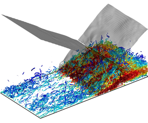


1 Introduction
The amplification of turbulence is a key feature in shock-wave/turbulence interaction (SWTI) and shock-wave/turbulent boundary layer interaction (SWTBLI), which is closely connected to flow separation, wall heat flux peak, skin friction and acoustic radiation in high-speed flows. A comprehensive understanding of the mechanism of turbulence amplification and an accurate prediction of turbulence statistics are of great importance to aerospace engineering. The linear interaction analysis (LIA) derived from the Euler equations, combined with the linearised Rankine–Hugoniot (R–H) jump relations, revealed some of the major characteristics of SWTI in the 1950s (Moore Reference Moore1954; Ribner Reference Ribner1954a,Reference Ribnerb; Kerrebrock Reference Kerrebrock1956; Chang Reference Chang1957), including the amplification of vorticity modes, the generation of acoustic and entropic waves, the distortion of the shock-wave front and the decrease of turbulence length scales. The LIA was then tested numerically for a wide range of Mach numbers and shock strengths by Zang, Hussaini & Bushnell (Reference Zang, Hussaini and Bushnell1984). Later, Barre, Alem & Bonnet (Reference Barre, Alem and Bonnet1996) conducted an experimental measurement of SWTI, and the amplification of turbulence was found to be in good agreement with LIA theory. Lee, Lele & Moin (Reference Lee, Lele and Moin1993, Reference Lee, Lele and Moin1997) conducted direct numerical simulation (DNS) of normal shock-wave/isotropic turbulence interactions in the 1990s, and their DNS agreed well with LIA in terms of the turbulence amplification ratio and change of turbulence length scale. Mahesh, Lele & Moin (Reference Mahesh, Lele and Moin1997) looked in particular at the variation in turbulence associated with shock-wave/entropy wave interaction and demonstrated the importance of the magnitude of entropy fluctuations and the correlation between velocity and temperature fluctuations with regard to the amplification of turbulence across the shock wave. In summary, LIA can be well applied in expressing and predicting the direct interaction between a shock wave and unbounded free turbulence, except for some nonlinear effects such as the rapid return to isotropy of the post-shock vorticity at high Reynolds numbers and the broken shock-wave surface identified in the DNS of Larsson & Lele (Reference Larsson and Lele2009) and Larsson, Bermejo-Moreno & Lele (Reference Larsson, Bermejo-Moreno and Lele2013).
Despite the success of LIA in SWTI problems, its application is quite limited in SWTBLI. Anyiwo & Bushnell (Reference Anyiwo and Bushnell1982) applied linear analysis to turbulence amplification mechanisms in SWTBLI and identified three aspects: the direct amplification of vortical modes across the shock wave, the generation of acoustic and entropy modes and the ‘pumping’ of turbulence from the mean flow by shock oscillation. Experimental research into a compression corner configuration by Smits & Muck (Reference Smits and Muck1987) indicated more complex mechanisms of turbulence amplification, including direct amplification across the shock wave, unsteady shock-wave oscillation and combined effects of adverse pressure gradient, compressive extra strain rates and concave curvature. These mechanisms are essentially nonlinear and cannot be captured or predicted by LIA. The experimental research of compression corners at Mach 2.9 of Zheltovodov & Yakovlev (Reference Zheltovodov and Yakovlev1986) and Zheltovodov, Lebiga & Yakovlev (Reference Zheltovodov, Lebiga and Yakovlev1989) also demonstrated turbulence amplification in the separated boundary layer across the shock wave. By using the method of diagrams of Kovaszhnay (Reference Kovaszhnay1953), they revealed the acoustic mode of the disturbances in the external flow above the separated shear layers. In particular, their experiments observed weak shocklets travelling downstream together with large-scale eddies in the separated shear layer. Some highlights can be found in the review paper of Zheltovodov (Reference Zheltovodov2006) and in the book chapter by Knight & Zheltovodov (Reference Knight, Zheltovodov, Babinsky and Harvey2011). Selig et al. (Reference Selig, Andreopoulos, Muck, Dussauge and Childs1989) conducted measurements in a  $24^{\circ }$ compression corner, and they suggested turbulence amplification in the upstream and downstream parts of the flow was dominated by the unsteady shock motion and large-scale Taylor–Görtler vortices in the detached shear layer. Measurements of turbulence amplification by Rose (Reference Rose1972) and Rose & Childs (Reference Rose and Childs1974) in an oblique shock-wave/flat-plate boundary layer interaction (OSWFPBLI) suggested the behaviour of turbulence in SWTBLI was in a non-equilibrium state and similar to those observed in an incompressible boundary layer with an adverse pressure gradient. Andreopoulos, Agui & Briassulis (Reference Andreopoulos, Agui and Briassulis2000) reviewed various kinds of shock-wave/turbulence interactions, and they argued that the turbulence amplification was not only affected by the shock interaction, but also by the unsteadiness of the shock system, the destabilising effect of the concave streamline curvature and the continuing downstream compression. In the recent measurements in OSWFPBLIs of Dupont et al. (Reference Dupont, Haddad, Ardissone and Debiève2005), Dupont, Haddad & Debiève (Reference Dupont, Haddad and Debiève2006) and Dupont, Piponniau & Dussauge (Reference Dupont, Piponniau and Dussauge2019), two separated maxima of amplified turbulence, especially for the streamwise velocity fluctuations, were identified. The first maximum is in the near-wall region immediately downstream of the reflected shock wave, and the second is away from the wall and preserved far downstream of the reattachment point. They attributed the second maximum to the free shear layer. Dupont et al. (Reference Dupont, Piponniau, Sidorenko and Debiève2008) adopted a particle image velocimetry measurement to study SWTBLI, and they confirmed that the high level of turbulence started from the near-wall region just downstream of the foot of the reflected shock, and moved upwards in the free shear layer. They also reported that the velocity profile in the detached free shear layer was similar to the mixing layer and attributed the strong turbulence in the free shear layer to a Kelvin–Helmholtz (K–H) instability. The detached free shear layer in SWTBLI is then further confirmed to be essentially a compressible mixing layer (Dupont et al. Reference Dupont, Piponniau and Dussauge2019).
Direct numerical simulation, which resolves the whole range of spatial and temporal scales of turbulence, has been applied to SWTBLI since 1998. The comprehensive data from these simulations have benefitted studies on turbulence amplification mechanisms greatly. Adams (Reference Adams1998, Reference Adams2000) conducted the first DNS of SWTBLI in an  $18^{\circ }$ compression corner, and a turbulence amplification factor of 4 was predicted, which was similar to the experiment of Smits & Muck (Reference Smits and Muck1987). However, according to Adams’s analysis, compressibility had no major effect on turbulence production, and the ‘pumping’ mechanism is also not relevant. Adams attributed this to the low Reynolds number in his simulation. Wu & Martín (Reference Wu and Martín2007, Reference Wu and Martín2008) conducted a DNS of a
 $24^{\circ }$ compression corner. Their DNS data were well validated against a wind tunnel experiment at low Reynolds numbers (Bookey, Wyckham & Smits Reference Bookey, Wyckham and Smits2005a,Reference Bookey, Wyckham and Smitsb), and a similar turbulence amplification factor to the experiment at a much higher Reynolds number was observed. They found that the maximum value of turbulence kinetic energy was located very close to the wall, and turbulence amplification was attributed to the comprehensive effects of an R–H jump across the shock wave, the nonlinear coupling of turbulence, vorticity and entropy waves and the unsteady shock-wave pumping effect. The same compression corner configuration was studied again by Priebe & Martín (Reference Priebe and Martín2012), and they proposed that the free shear layer in the SWTBLI is similar to the plane mixing layer with a single inflection point in the velocity profile. They also reported that the maximum turbulence kinetic energy occurred in the middle of the free shear layer, and they further attributed the turbulence amplification to the formation of energetic turbulent structures in the separated shear layer and subsequent shedding of these structures into the downstream. The DNS data of Priebe & Martín (Reference Priebe and Martín2012) were analysed by Helm, Martin & Dupont (Reference Helm, Martin and Dupont2014), focusing on the free shear layer. They observed a linear growth of the free shear layer and large-scale vortices due to the K–H instability. The generation of large-scale vortices in the free shear layer (i.e. the mixing layer) was believed to be a major mechanism for turbulence amplification in SWTBLI. Li et al. (Reference Li, Fu, Ma and Liang2010) analysed the turbulence kinetic energy transport equation in the same
 $24^{\circ }$ compression corner flow, and they observed that turbulence kinetic energy production was mainly due to the shear of the mean flow, and the compression effect was relatively weak. Compression corner flows with different turning angles were then studied by Tong et al. (Reference Tong, Yu, Tang and Li2017) using DNS. They confirmed that the intensity of turbulence fluctuations was amplified greatly by the shock wave, and an analysis of the turbulence kinetic energy budgets showed the peak values of the turbulence kinetic energy production and dissipation are in the near-wall region. It was suggested that the turbulence kinetic energy transport characteristic in the SWTBLI was similar to that observed in a canonical flat-plate boundary layer, although the turbulence was highly amplified. They also presented large-scale hairpin vortices and packets in the free shear layer and the destruction of streaky structures in the near-wall region.
Pirozzoli & Grasso (Reference Pirozzoli and Grasso2006) conducted the first DNS of an OSWFPBLI configuration at Mach 2.25. This configuration is more favourable for the investigation of turbulence amplification mechanisms since the curvature of the wall is avoided. They found that the turbulence was amplified in the mixing layer with its largest values away from the wall. Both the turbulence kinetic energy and its production term were found to reach their maxima inside the mixing layer. Therefore, they concluded that the formation of the mixing layer was primarily responsible for the amplification of turbulence. The large-scale low-frequency unsteadiness of the shock wave was also identified in their DNS, although they did not take this to be a major turbulence amplifier. Subsequently, Pirozzoli, Bernardini & Grasso (Reference Pirozzoli, Bernardini and Grasso2010) reported the same turbulence amplification mechanism in a transonic SWTBLI. In a more recent DNS of OSWFPBLI, Pirozzoli & Bernardini (Reference Pirozzoli and Bernardini2011) confirmed again that the maximum production of turbulence kinetic energy in SWTBLI is owing to the lift-up of vortical structures in the mixing layer. Priebe, Wu & Martín (Reference Priebe, Wu and Martín2009) also studied an OSWFPBLI flow at a Mach number 2.9. Their DNS showed a lower amplification of the mass-flux turbulence intensity than the compression corner configuration at the same inflow conditions, due to the concave streamline curvature missing in a flat-plate configuration. Similar to the DNS of Pirozzoli & Grasso (Reference Pirozzoli and Grasso2006), they also identified that the peak of the turbulence intensity was in the detached shear layer, implying a similar mixing-layer mechanism for the turbulence amplification. Sandham (Reference Sandham2016) recently analysed the effects of compressibility on turbulence in SWTBLI, and argued that the turbulence in the outer part of the boundary layer might be similar to shock-wave/turbulence interaction, and the changes of turbulence inside the boundary layer were dominated by the free shear layer, which confirmed the mixing-layer mechanism for turbulence amplification. He also noticed the peak shear stress did not align with that of the streamwise velocity fluctuations and proposed that it was due to curvature effects, which has a strong impact on streamwise velocity fluctuations but not so much on wall-normal or spanwise velocity fluctuations.
It can be summarised that the LIA works well in expressing turbulence amplification in shock-wave/free turbulence interaction. However, its application in SWTBLI is less successful. The amplification of turbulence in SWTBLI is much more complicated and essentially nonlinear. The history of research of turbulence amplification in SWTBLI can be divided into two stages. In the early stage (1950s–2000s), many factors (e.g. unsteady shock-wave movement, direct shock-wave/turbulence interaction, generation of acoustic and entropy waves and a free shear layer) were considered to make contributions to the turbulence amplification, but the key factor could not be identified. In the latter stage (2000s–present), due to the application of advanced experimental technologies (e.g. particle image velocimetry) and high-fidelity simulations (e.g. DNS and large-eddy simulation) in the research of high-speed flow, some less important factors were excluded, and the free shear layer was believed to be the key factor for the amplification of turbulence, based on the observation that the maximum turbulence energy and turbulence kinetic energy production are located far away from the wall. The free shear layer was then further studied and confirmed to be the main factor for the amplification of turbulence in SWTBLI, and its physics was explained as a K–H instability. In the present paper, we propose that there is an additional mechanism for the amplification of turbulence in SWTBLI, apart from the K–H instability of the free shear layer, and this new mechanism is responsible for the rapid growth of turbulent energy in the interaction zone. Compared with free shear layer, this mechanism takes effect only in a limited region, which might be the reason that it was ignored in the previous studies, but its contribution to the amplification of turbulence is significant, and it reveals that the amplification of turbulence in the initial part of the interaction zone is not essentially shear driven. Indeed, several research articles have reported high turbulence intensity in the near-wall region close to the foot of the reflected shock wave both experimentally (Dupont et al. Reference Dupont, Piponniau, Sidorenko and Debiève2008) and numerically (Wu & Martín Reference Wu and Martín2007; Li et al. Reference Li, Fu, Ma and Liang2010). Two separated turbulence kinetic energy maxima in the near-wall region and outer part of the boundary layer were also observed (Dupont et al. Reference Dupont, Haddad, Ardissone and Debiève2005, Reference Dupont, Haddad and Debiève2006, Reference Dupont, Piponniau and Dussauge2019). The new turbulence amplification mechanism proposed in the present paper will provide a clear physical explanation for these observations.
In the present paper, a baseline OSWFPBLI case of a  $33.2^{\circ }$ impinging shock-wave/turbulent boundary layer interaction at Mach 2.25 is studied using DNS. The flow parameters are similar to the DNS of Pirozzoli & Grasso (Reference Pirozzoli and Grasso2006), but the mesh is finer in the present simulation to capture small-scale structures where turbulence is amplified. The results are validated against available experimental data and other DNS, and our DNS data are analysed in full with a specific focus on turbulence amplification mechanism. The present study is structured as follows: the DNS of the SWTBLI flow is presented in § 2, including the computational set-up, the validation of the results and the preliminary analysis of the flow field. The turbulence amplification mechanism is focused on in § 3, through the analysis of the Reynolds stress, shear layer, turbulence kinetic energy budgets, pressure fluctuations and turbulence structures. Concluding remarks are given in § 4.
2 DNS of SWTBLI
2.1 Computational set-up
The three-dimensional (3-D) unsteady compressible Navier–Stokes equations in a non-dimensional form are solved numerically using a high-order finite difference method in a generalised coordinate system. The convection terms are solved with a seventh-order low-dissipative monotonicity-preserving (MP7-LD) scheme (Fang, Li & Lu Reference Fang, Li and Lu2013; Fang et al. Reference Fang, Yao, Li and Lu2014), which can resolve small-scale turbulent structures as effectively as high-order central schemes, whilst preserving monotonicity near shock waves. This approach has been recently applied to studies of various SWTBLI problems (see Fang et al. Reference Fang, Yao, Li and Lu2014, Reference Fang, Yao, Zheltovodov, Li and Lu2015, Reference Fang, Yao, Zheltovodov and Lu2017). The diffusion terms are solved using a sixth-order compact central scheme (Hirsh Reference Hirsh1975; Lele Reference Lele1992) with a domain decoupling scheme for parallel computation (Fang et al. Reference Fang, Gao, Moulinec and Emerson2019). After all the spatial terms are solved, a three-step third-order total variation diminishing Runge–Kutta method, proposed by Gottlieb & Shu (Reference Gottlieb and Shu1998), is used for the temporal integration. The thermodynamic relation is specified by the ideal gas law, with the ratio of specific heats,  $\unicode[STIX]{x1D6FE}=1.4$ and the gas constant,
 $R=287.1~\text{J}~\text{kg}^{-1}~\text{K}^{-1}$. The dynamic viscosity coefficient is calculated based on the temperature,
 $T$, using Sutherland’s law,
 $\unicode[STIX]{x1D707}=C_{1}T^{1.5}/(T_{S}+T)$, with the coefficient
 $C_{1}=1.458\times 10^{-6}~\text{kg}~\text{m}^{-1}~\text{s}^{-1}~\text{k}^{-1/2}$ and the Sutherland temperature,
 $T_{S}=110.3~\text{K}$. A constant Prandtl number,
 $Pr=0.72$, is used in the present study.
A two-dimensional sketch of the computational domain and set-up. BL, boundary layer.

Summary of mesh resolution and boundary layer parameters. All parameters are selected at the reference station, exception for  $\unicode[STIX]{x0394}x_{min}^{+}$, which is the global minimum value. The superscript ‘
 $+$’ stands for variables in wall units. In the
 $y$-direction,
 $\unicode[STIX]{x0394}y_{1}^{+}$ and
 $\unicode[STIX]{x0394}y_{e}^{+}$ are, respectively, the wall-normal mesh resolutions at the first point off the wall and the edge of the boundary layer. The Reynolds number,
 $Re_{\unicode[STIX]{x1D6FF}}$,
 $Re_{\unicode[STIX]{x1D6FF}^{\ast }}$ and
 $Re_{\unicode[STIX]{x1D703}}$ are, respectively, the Reynolds numbers based on the nominal, displacement and momentum thicknesses of the boundary layer.

A two-dimensional cross-section of the computational domain is sketched in figure 1. The domain starts from a laminar boundary layer, and wall blowing and suction are introduced on the wall to trigger a boundary layer transition so that a fully developed turbulent boundary layer is established upstream of the interaction zone. The Mach number of the incoming free-stream flow is  $Ma=2.25$, and the Reynolds number, based on the nominal boundary layer thickness at the inlet plane,
 $\unicode[STIX]{x1D6FF}_{0}$, is
 $Re_{\unicode[STIX]{x1D6FF}_{0}}=\unicode[STIX]{x1D70C}_{\infty }u_{\infty }\unicode[STIX]{x1D6FF}_{0}/\unicode[STIX]{x1D707}_{\infty }=11\,277$, where
 $\unicode[STIX]{x1D70C}$,
 $u$ and
 $\unicode[STIX]{x1D707}$ are, respectively, the density, velocity and viscosity of the flow and the subscript,
 $\infty$, represents a variable in the incoming free-stream flow. Note that
 $x$,
 $y$ and
 $z$ are, respectively, the streamwise, wall-normal and spanwise coordinates, and
 $u$,
 $v$ and
 $w$ are the three velocity components in the
 $x$,
 $y$ and
 $z$ directions. The origin of the coordinate system is set at the inviscid shock-wave impinging point at the wall, and the reference station is selected at
 $x=-4\unicode[STIX]{x1D6FF}_{ref}$, where the flow is a fully developed undisturbed turbulent boundary layer, and
 $\unicode[STIX]{x1D6FF}_{ref}$ is the nominal boundary layer thickness at the reference station. The nominal boundary layer thickness,
 $\unicode[STIX]{x1D6FF}$, is defined as the vertical distance from the walls to a point where the flow velocity has reached
 $0.99u_{\infty }$. Unless otherwise notified, the length scales in the analysis of the results are all normalised by
 $\unicode[STIX]{x1D6FF}_{ref}$, and the velocity scales are all normalised by the incoming free-stream velocity,
 $u_{\infty }$. The computational domain is a
 $85.1\times 10.5\times 1.85$ cuboid and discretised with a
 $4020\times 220\times 256$ Cartesian mesh. The mesh is refined in the near-wall region and the interaction zone to capture possible small-scale turbulent structures, and the mesh is uniformly distributed in the spanwise direction. The spanwise width of the domain is approximately
 $L_{z}=1.85\unicode[STIX]{x1D6FF}_{ref}$ (
 $L_{z}^{+}=1440$ in local wall units), which is a typical value used in many studies of SWTBLI flows (see, e.g. Pirozzoli & Grasso Reference Pirozzoli and Grasso2006; Pirozzoli et al. Reference Pirozzoli, Bernardini and Grasso2010; Priebe & Martín Reference Priebe and Martín2012; Jammalamadaka, Li & Jaberi Reference Jammalamadaka, Li and Jaberi2013; Tong et al. Reference Tong, Yu, Tang and Li2017). The information of the domain and the mesh resolution is presented in table 1.
A laminar boundary layer profile obtained from a compressible Blasius solution is prescribed at the inlet plane, and a supersonic inflow boundary condition is applied, except for the subsonic portion of the boundary layer where an extrapolation of pressure is used. At the outlet and far-field boundaries, characteristic boundary conditions for the N–S equations proposed by Poinsot & Lele (Reference Poinsot and Lele1992) and extended to generalised coordinates by Kim & Lee (Reference Kim and Lee2000, Reference Kim and Lee2004) are adopted. At the far-field boundary, the single-point R–H relations are used to specify the free-stream values before and after the impinging shock wave, and the reflected shock wave goes out of the domain through the outlet boundary. To further reduce any reflections from the outlet boundary, an additional sponge zone with a stretched mesh and a second-order filter (Gloerfelt & Lafon Reference Gloerfelt and Lafon2008) is incorporated near the outlet boundary to drive the flow towards a uniform state. At the wall, an isothermal non-slip boundary condition with a fixed wall temperature,  $T_{w}=1.9T_{0}$, is applied, except for the blowing and suction region, where the wall-normal velocity,
 $v_{bs}$, is applied from
 $x_{a}=-74$ to
 $x_{b}=-62$, by the following formula:
 $$\begin{eqnarray}v_{bs}=A_{bs}\,f_{bs}(x)g_{bs}(z)h_{bs}(t).\end{eqnarray}$$
In the above equation, (2.1), the intensity of the blowing and suction is assigned as  $A_{bs}=0.04$, and
 $f_{bs}(x)$,
 $g_{bs}(z)$ and
 $h_{bs}(t)$ define the variations of the wall-normal fluctuations in the streamwise direction, spanwise direction and time,
 $t$, respectively. According to the early DNS of the compressible boundary layer of Rai, Gatski & Erlebacher (Reference Rai, Gatski and Erlebacher1995), Pirozzoli, Grasso & Gatski (Reference Pirozzoli, Grasso and Gatski2004) and Gao et al. (Reference Gao, Fu, Ma and Li2005), the detailed expressions for
 $f_{bs}(x)$,
 $g_{bs}(z)$ and
 $h_{bs}(t)$ are given as
 $$\begin{eqnarray}\left.\begin{array}{@{}c@{}}f_{bs}(x)={\displaystyle \frac{4}{\sqrt{27}}}\sin \left(2\unicode[STIX]{x03C0}{\displaystyle \frac{x-x_{a}}{x_{b}-x_{a}}}\right)\left(1-\cos \left(2\unicode[STIX]{x03C0}{\displaystyle \frac{x-x_{a}}{x_{b}-x_{a}}}\right)\right),\\ g_{bs}(z)=\displaystyle \mathop{\sum }_{n=1}^{10}0.8^{n-1}g_{0}\sin \left[2\unicode[STIX]{x03C0}n\left({\displaystyle \frac{z}{L_{z}}}+\unicode[STIX]{x1D711}_{n}\right)\right],\\ h_{bs}(t)=\displaystyle \mathop{\sum }_{m=1}^{5}0.8^{m-1}h_{0}\sin [2\unicode[STIX]{x03C0}m(\unicode[STIX]{x1D6FD}t+\unicode[STIX]{x1D711}_{m})],\end{array}\right\}\end{eqnarray}$$
where  $g_{0}=1/\sum _{n=1}^{10}0.8^{n-1}$ and
 $h_{0}=1/\sum _{m=1}^{5}0.8^{m-1}$. The basic frequency of the wall blowing and suction is set as
 $\unicode[STIX]{x1D6FD}=0.2u_{\infty }/\unicode[STIX]{x1D6FF}_{ref}$, and the phase parameters,
 $\unicode[STIX]{x1D711}_{n}$ and
 $\unicode[STIX]{x1D711}_{m}$, are random numbers ranging from 0 to 1. In the present study, the wall fluctuations have two modes in the streamwise direction, ten modes in the spanwise direction and five temporal modes. The net flow rate of the wall blowing and suction is zero in the simulation so that there is no extra mass flux introduced to the flow field from the wall. A periodic condition is used in the spanwise direction.
2.2 Validation
The streamwise mean velocity,  $\langle u\rangle$, in the outer scaling and the inner scaling at the reference station are shown in figure 2, in which
 $u_{VD}$ is the van Driest transformed velocity, defined as
 $$\begin{eqnarray}u_{VD}=\int _{0}^{\langle u\rangle }\frac{\overline{\unicode[STIX]{x1D70C}}}{\overline{\unicode[STIX]{x1D70C}}_{w}}\,\text{d}\langle u\rangle ,\end{eqnarray}$$
where the subscript,  $w$, represents variables at the wall, and
 $\overline{\phantom{0}}$ and
 $\left\langle \right\rangle$ stand for the Reynolds-averaged and Favre-averaged variables, respectively. The averaging operations in the present study are conducted in both time and spanwise direction. In figure 2(a), the mean velocity profile in the undisturbed boundary layer of the present DNS matches well with the measured data of Shutts, Hartwig & Weiler (Reference Shutts, Hartwig and Weiler1955) at a
 $Ma=2.25$ boundary layer and Bookey et al. (Reference Bookey, Wyckham and Smits2005a) at a
 $Ma=2.9$ boundary layer. In figure 2(b), a good agreement of the velocity profile with the classic law of the wall and the data from the DNS of incompressible boundary layers (Wu & Moin Reference Wu and Moin2009; Schlatter & Orlu Reference Schlatter and Orlu2010) in the inner and log layers can be confirmed. The difference in the wake layer is due to the Reynolds number and compressibility effects (Wenzel et al. Reference Wenzel, Selent, Kloker and Rist2018).
The profiles of the density-scaled Reynolds stress components  $\overline{\unicode[STIX]{x1D70C}}/\overline{\unicode[STIX]{x1D70C}}_{w}\langle u^{\prime \prime }u^{\prime \prime }\rangle$,
 $\overline{\unicode[STIX]{x1D70C}}/\overline{\unicode[STIX]{x1D70C}}_{w}\langle v^{\prime \prime }v^{\prime \prime }\rangle$,
 $\overline{\unicode[STIX]{x1D70C}}/\overline{\unicode[STIX]{x1D70C}}_{w}\langle w^{\prime \prime }w^{\prime \prime }\rangle$ and
 $\overline{\unicode[STIX]{x1D70C}}/\overline{\unicode[STIX]{x1D70C}}_{w}\langle u^{\prime \prime }v^{\prime \prime }\rangle$ at the reference station are plotted in figure 3, and the superscript,
 $^{\prime \prime }$, stands for the fluctuation from a Favre-averaged variable. Good qualitative agreement between the present study and the DNS data of the incompressible boundary layer of Schlatter & Orlu (Reference Schlatter and Orlu2010) is achieved after the Reynolds stresses are scaled by the density profile.
The mean velocity profile in the outer scaling (a) and the van Driest transformed mean streamwise velocity station in the inner scaling (b) at the reference station,  $x=-4\unicode[STIX]{x1D6FF}_{ref}$. The superscript,
 $^{+}$, stands for a variable in wall units.

The density-scaled Reynolds stress in outer scaling (a) and inner scaling (b) at the reference station. Lines are the present results and symbols are the results of incompressible DNS of Schlatter & Orlu (Reference Schlatter and Orlu2010).

The spanwise two-point correlations of velocity fluctuations at the reference station are presented in figure 4 to verify if the width of the computational domain is large enough to decorrelate fluctuations. The spanwise two-point correlation of velocity fluctuations,  $u_{i}^{\prime \prime }$, is defined as
 $$\begin{eqnarray}C_{u_{i}u_{i}}^{z}(x,y,\unicode[STIX]{x0394}z)=\frac{\overline{u_{i}^{\prime \prime }(x,y,z)u_{i}^{\prime \prime }(x,y,z+\unicode[STIX]{x0394}z)}}{\overline{u_{i}^{\prime \prime }(x,y,z)u_{i}^{\prime \prime }(x,y,z)}}.\end{eqnarray}$$
The correlations of velocity fluctuations from the near-wall region to the edge of the boundary layer are examined in figure 4, and the DNS of channel flow at  $Re_{\unicode[STIX]{x1D70F}}=590$ (
 $Re_{\unicode[STIX]{x1D70F}}$ is the friction Reynolds number based on the wall friction velocity) of Moser, Kim & Mansour (Reference Moser, Kim and Mansour1999) is used to validate the result in the near-wall region. In figure 4, we can see that the spanwise two-point correlations of velocity fluctuations at all positions are close to zero when the spanwise distance of the two points approaches the half-width of the domain, confirming the domain is wide enough to decorrelate the resolved fluctuations. The correlations in the near-wall region agree well with the data in the incompressible channel flow, indicating that turbulence in the near-wall region of a supersonic turbulent boundary layer is essentially incompressible.
The spanwise two-point correlations of streamwise, wall-normal and spanwise velocity fluctuations at the reference station.

The mean wall pressure,  $(\overline{p}_{w}-p_{\infty })/(p_{1}-p_{\infty })$, and root-mean-square (r.m.s.) wall pressure fluctuations,
 $\sqrt{\overline{p_{w}^{\prime 2}}}/(p_{1}-p_{\infty })$, are compared with the experimental data of Dupont et al. (Reference Dupont, Haddad and Debiève2006) at
 $Ma=2.3$ and
 $Re_{\unicode[STIX]{x1D703}}=6900$ in figure 5. The pressure after the reflective shock wave,
 $p_{1}$, is determined by the R–H jump relation, and the superscript,
 $^{\prime }$, stands for the fluctuation from a Reynolds-averaged variable. The DNS result is compared with the experimental case with an
 $8^{\circ }$ wedged shock generator, which generated a
 $32.4^{\circ }$ impinging shock wave. The origin of the
 $x$-axis in figure 5 is set as the mean position of the foot of the reflected shock wave,
 $x_{RS}$, which was deduced from the schlieren visualisation in the experiment, but determined as the position where the mean wall pressure,
 $\overline{p}_{w}$, rises to
 $(p_{1}+p_{\infty })/2$ in the DNS, as demonstrated in figure 5(a). A good agreement of the mean wall pressure between the DNS and the experimental data can be confirmed in figure 5(a). Compared with the result of the inviscid interaction, we can observe the effect of the viscous boundary layer, which spreads the wall pressure jump into a much larger area with a smoother pressure gradient.
Distributions of mean wall pressure (a) and r.m.s. wall pressure fluctuations (b) scaled by the pressure difference before and after the reflected shock wave. The origin of the  $x$-axis is shifted to the mean position of the foot of the reflected shock wave.

The level of wall pressure fluctuations in the undisturbed boundary layer is maintained to a level of  $\sqrt{\overline{p_{w}^{\prime 2}}}=2.60\unicode[STIX]{x1D70F}_{w}$, in which the wall shear stress,
 $\unicode[STIX]{x1D70F}_{w}$, is calculated as
 $\unicode[STIX]{x1D70F}_{w}=\unicode[STIX]{x1D707}_{w}(\unicode[STIX]{x2202}u/\unicode[STIX]{x2202}y)|_{w}$. The value is close to the wall pressure fluctuations of
 $\sqrt{\overline{p_{w}^{\prime 2}}}=2.55\unicode[STIX]{x1D70F}_{w}$ in a low-speed boundary layer measured by Farabee & Casarella (Reference Farabee and Casarella1991) and
 $\sqrt{\overline{p_{w}^{\prime 2}}}=2.50\unicode[STIX]{x1D70F}_{w}$ reported in a DNS of a transonic SWTBLI by Bernardini, Pirozzoli & Grasso (Reference Bernardini, Pirozzoli and Grasso2011). In the interaction region, the r.m.s. wall pressure fluctuations in figure 5(b) shows a steep increase with the rise of the mean wall pressure, and it reaches a peak around the foot of the impinging shock. The maximal pressure sound level is increased by 13.4 dB.
A comparison of the wall pressure fluctuations between the DNS and experiment shows good agreement in terms of the trends of the two results, but the DNS predicts a higher level of the wall pressure fluctuations than the measurement in both the undisturbed boundary layer and the interaction region. Dupont et al. (Reference Dupont, Haddad and Debiève2006) have indicated that their measured r.m.s. wall pressure fluctuations were much lower than other experiments, and they attributed it to the low cutoff frequency of the pressure transducers used for their measurements. By shifting the DNS result to match the level of wall pressure fluctuations upstream the interaction region in figure 5(b) as the compensation of underestimation of the pressure fluctuations in the experiment, we can then observe a good agreement between the DNS and the experimental data.
2.3 Characteristics of the flow separation
The profiles of the mean wall skin-friction coefficient,  $C_{f}=\unicode[STIX]{x1D70F}_{w}/((1/2)\unicode[STIX]{x1D70C}_{\infty }u_{\infty }^{2})$, and the probability of negative skin friction,
 $\unicode[STIX]{x1D6FE}_{\unicode[STIX]{x1D70F}_{w}}$, defined as the fraction of total time when the instantaneous skin-friction coefficient is negative, are presented in figure 6. After entering the interaction zone, the skin friction drops with the increase of the mean wall pressure (as shown in figure 5a), representing a boundary layer deceleration under an adverse pressure gradient condition. In contrast to the DNS of Pirozzoli & Grasso (Reference Pirozzoli and Grasso2006), the present study predicts two distinct separation zones. The skin friction drops sharply and becomes negative before rising to a positive value. We refer to this as the secondary separation zone. After this brief rise, the skin friction again reduces to a negative value before increasing to positive values. This region is referred to as the primary separation zone. The secondary and primary separation–reattachment lines are marked in figure 6 as S1–R1 and S2–R2, respectively. A similar skin-friction distribution was also observed in a recent large-eddy simulation by Vyas, Yoder & Gaitonde (Reference Vyas, Yoder and Gaitonde2019). In the DNS of a compression corner flow of Priebe & Martín (Reference Priebe and Martín2012), the two separated zones of negative skin friction were also reported at the collapsing phase of the separation bubble. According to the probability of reverse flow at the wall,
 $\unicode[STIX]{x1D6FE}_{\unicode[STIX]{x1D70F}_{w}}$, the mean separation and reattachment points correspond to the locations of
 $\unicode[STIX]{x1D6FE}_{\unicode[STIX]{x1D70F}_{w}}=0.5$, confirming the occurrence of the two separation bubbles.
Distribution of the skin-friction coefficient and the probability of negative skin friction,  $\unicode[STIX]{x1D6FE}_{\unicode[STIX]{x1D70F}_{w}}$, at the wall.

The probability of reverse flow,  $\unicode[STIX]{x1D6FE}_{u}$, defined as the fraction of total time when the instantaneous streamwise velocity,
 $u$, is negative (Simpson Reference Simpson1981, Reference Simpson1989), is used to further analyse the separation bubble in the
 $x{-}y$ plane in figure 7. The streamwise location of
 $\unicode[STIX]{x1D6FE}_{u}=0.5$ indicates the occurrence of mean flow separation or reattachment, and the flow detachment can be characterised as incipient detachment, intermittent transitory detachment and transitory detachment based on
 $\unicode[STIX]{x1D6FE}_{u}=0.01$, 0.2, and 0.5, respectively (Simpson Reference Simpson1989; Tong et al. Reference Tong, Yu, Tang and Li2017). From figure 7, the two separation bubbles can be identified. It is worthwhile to mention that the maximum value of
 $\unicode[STIX]{x1D6FE}_{u}$ is approximately 0.63, meaning there is no permanent reverse flow for the case studied here.
Probability of reverse flow,  $\unicode[STIX]{x1D6FE}_{u}$. The incipient detachment, intermittent transitory detachment and transitory detachment lines are identified as dash contour lines.

Mean streamlines and pressure field (a) and instantaneous streamwise velocity (b) in the  $x{-}y$ plane. The mean pressure in (a) is normalised by the free-stream pressure, and the red lines in (b) are the
 $u=0$ contours. The extension line of the impinging shock wave is plotted with a thin dashed line in (b) and following figures.

The mean pressure field with mean streamlines and instantaneous streamwise velocity field in the  $x{-}y$ plane are shown in figure 8, which reveals details of the flow separation. The mean pressure rises inside the boundary layer through a series of compression waves. A small and thin separation zone is identified immediately downstream where the pressure starts to rise, producing a sharp tip ahead of the main separation zone. A similar shape of the separation bubble can also be seen in the result of Touber & Sandham (Reference Touber and Sandham2009, Reference Touber and Sandham2011). A large area of instantaneous reverse flow in the gap between the two separation zones can be observed in figure 8(b), meaning the separation flow in the interaction zone is strongly intermittent, and the appearance of the two separation zones should be a case-dependent scenario.
3 Turbulence amplification mechanism
3.1 Reynolds stress
The Reynolds stress components  $\langle u^{\prime \prime }u^{\prime \prime }\rangle$,
 $\langle v^{\prime \prime }v^{\prime \prime }\rangle$,
 $\langle w^{\prime \prime }w^{\prime \prime }\rangle$,
 $\langle u^{\prime \prime }v^{\prime \prime }\rangle$ and turbulent kinetic energy, defined as
 $$\begin{eqnarray}K=0.5[\langle u^{\prime \prime }u^{\prime \prime }\rangle +\langle v^{\prime \prime }v^{\prime \prime }\rangle +\langle w^{\prime \prime }w^{\prime \prime }\rangle ],\end{eqnarray}$$
are presented in figure 9, together with their peak locations in the streamwise direction. The peak is defined as the local maximum along the wall-normal direction at an  $x$-station. The main characteristic is the amplification of all the Reynolds stress components with their peaks moving from the near-wall region to the core of the free shear layer or mixing layer, which has been reported previously (Dupont et al. Reference Dupont, Haddad, Ardissone and Debiève2005, Reference Dupont, Haddad and Debiève2006, Reference Dupont, Piponniau, Sidorenko and Debiève2008, Reference Dupont, Piponniau and Dussauge2019; Pirozzoli & Grasso Reference Pirozzoli and Grasso2006; Wu & Martín Reference Wu and Martín2007; Li et al. Reference Li, Fu, Ma and Liang2010; Pirozzoli & Bernardini Reference Pirozzoli and Bernardini2011; Priebe & Martín Reference Priebe and Martín2012; Helm et al. Reference Helm, Martin and Dupont2014) as evidence of the turbulence amplification mechanism due to the free shear layer.
Reynolds stress components  $\langle u^{\prime \prime }u^{\prime \prime }\rangle$ (a),
 $\langle v^{\prime \prime }v^{\prime \prime }\rangle$ (b),
 $\langle w^{\prime \prime }w^{\prime \prime }\rangle$ (c),
 $\langle u^{\prime \prime }v^{\prime \prime }\rangle$ (d) and
 $K$ (e). All the variables are normalised by the square of the friction velocity at the reference station. The green thick lines mark the peaks of each variable.

The amplification factor of a variable,  $f$, at a streamwise location,
 $x$, is defined as
 $$\begin{eqnarray}\unicode[STIX]{x1D711}_{f}(x)=\frac{\unicode[STIX]{x1D6EC}_{f}(x)}{\unicode[STIX]{x1D6EC}_{f}(x_{ref})},\end{eqnarray}$$
where  $\unicode[STIX]{x1D6EC}_{f}(x)$ is the peak value of the variable
 $f$ at an
 $x$-position. The maximum amplification factors of Reynolds stress and turbulent kinetic energy are listed in table 2. Turbulence kinetic energy is amplified by a factor of 2.97, which is close to 2.7 in the DNS of Pirozzoli & Grasso (Reference Pirozzoli and Grasso2006). The peaks of Reynolds stress are plotted together with mean streamlines in figure 10. It can be seen that the peaks of Reynolds stress follow the streamlines during the initial amplification of turbulence until they reach the crest of the separation bubble. As we move downstream, the mean streamlines turn back towards the wall and the peaks of Reynolds stress continue moving outwards. Consequently, we observe the deviation between the tracks of Reynolds stress peaks and the mean streamlines, consistent with the observation of Sandham (Reference Sandham2016).
Mean streamlines (black line with arrows) and peaks of the Reynolds stress. The peaks  $\langle u^{\prime \prime }u^{\prime \prime }\rangle$,
 $\langle v^{\prime \prime }v^{\prime \prime }\rangle$,
 $\langle w^{\prime \prime }w^{\prime \prime }\rangle$ and
 $K$ are, respectively, marked with red, green, blue and purple lines.

Maximum amplification factors of the Reynolds stress and turbulence kinetic energy and their coordinates.

The spatial evolutions of the amplification factors of Reynolds stress and the vertical positions of the peaks of the Reynolds stress,  $y_{peak}$, are plotted in figure 11. Upstream of the interaction region, the peaks are positioned well in the near-wall region, demonstrating equilibrium wall turbulence. When entering the interaction zone, all the peaks move away from the wall, indicating the creation of a detached free shear layer. The free shear layer starts to decay and diffuse after being developed, leading to slow damping of the Reynolds stress.
Evolution of the amplification factors of Reynolds stress (a) and the distance of Reynolds stress peaks to the wall (b). The solid circles mark the global maxima of the corresponding Reynolds stress components.

Up to now, the observations support the explanation of the turbulence amplification due to the free shear layer. However, by a detailed analysis of the evolution of the peaks in figure 11, we notice that the global maxima of Reynolds stress, marked as solid circles in the figure, are reached at locations where the free shear layer is not yet fully detached. Their global maxima are not positioned away from the wall. The peak of  $\langle u^{\prime \prime }u^{\prime \prime }\rangle$ is amplified at a location more upstream than the other two components, and its peak position stays in the near-wall region during its amplification process.
The peaks of the three components of Reynolds stress are further highlighted in figure 12. At the reference station, the peak of  $\langle u^{\prime \prime }u^{\prime \prime }\rangle$ is at
 $y_{peak}=0.016\unicode[STIX]{x1D6FF}_{ref}$ (
 $\,y_{peak}^{+}=12$), which agrees with the location of the maximum streamwise velocity fluctuations in the incompressible channel flow reported by Kim, Moin & Moser (Reference Kim, Moin and Moser1987). The maximum production of turbulence and strongest ejection and sweep events were also found at the location of
 $y^{+}=12$ in the incompressible channel flow. The peak of
 $\langle u^{\prime \prime }u^{\prime \prime }\rangle$ is then amplified by 50 % at
 $x=-2.18$ with its position barely moved (
 $\,y_{peak}=0.017\unicode[STIX]{x1D6FF}_{ref}$). Further downstream, the value of
 $\langle u^{\prime \prime }u^{\prime \prime }\rangle$ peak is doubled at
 $x=-2.02$, and its peak is still in the inner region of the boundary layer (
 $\,y_{peak}=0.02\unicode[STIX]{x1D6FF}_{ref}$), and the global maximum of
 $\langle u^{\prime \prime }u^{\prime \prime }\rangle$ is achieved at
 $x=-1.76$ with its wall-normal position at
 $y_{peak}=0.04\unicode[STIX]{x1D6FF}_{ref}$, where
 $\langle u^{\prime \prime }u^{\prime \prime }\rangle$ is amplified by 140 %. The near-wall peak of Reynolds stress was also observed in the experiment of Dupont et al. (Reference Dupont, Haddad, Ardissone and Debiève2005), Dupont et al. (Reference Dupont, Haddad and Debiève2006), Dupont et al. (Reference Dupont, Piponniau, Sidorenko and Debiève2008) and Dupont et al. (Reference Dupont, Piponniau and Dussauge2019), and therefore we suspect that the amplification of turbulence, at least for
 $\langle u^{\prime \prime }u^{\prime \prime }\rangle$, may not be due to the free shear layer detached from the mean separation position.
Distribution of the amplification factors of Reynolds stress and the vertical distance of Reynolds stress peaks from the wall. The symbols mark the global maxima of the corresponding Reynolds stress components.

For the other two components,  $\langle v^{\prime \prime }v^{\prime \prime }\rangle$ and
 $\langle w^{\prime \prime }w^{\prime \prime }\rangle$, the amplification is delayed compared to
 $\langle u^{\prime \prime }u^{\prime \prime }\rangle$. The peak of
 $\langle v^{\prime \prime }v^{\prime \prime }\rangle$ reaches a maximum at
 $x=-1.24$ with its position at
 $y_{peak}=0.11\unicode[STIX]{x1D6FF}_{ref}$, and the peak of
 $\langle w^{\prime \prime }w^{\prime \prime }\rangle$ reaches its maximum at
 $x=-1.5$ with its position at
 $y_{peak}=0.067\unicode[STIX]{x1D6FF}_{ref}$. Considering the core of the free shear layer will finally reach a height of
 $y=0.2\unicode[STIX]{x1D6FF}_{ref}{-}0.3\unicode[STIX]{x1D6FF}_{ref}$, it would appear that the amplification of turbulence mainly occurs in the inner region of the boundary layer, especially for the streamwise velocity fluctuations.
3.2 Shear layer
The two-dimensional shear layer is measured using the mean spanwise vorticity,  $\unicode[STIX]{x1D714}_{z}=\unicode[STIX]{x2202}\langle v\rangle /\unicode[STIX]{x2202}x-\unicode[STIX]{x2202}\langle u\rangle /\unicode[STIX]{x2202}y$, (Priebe & Martín Reference Priebe and Martín2012; Helm et al. Reference Helm, Martin and Dupont2014), as presented in figure 13. It can be seen that the shear layer starts to detach from the wall in the interaction zone, and its core gets further away from the wall as the flow progresses downstream. The core of the free shear layer reaches a height of approximately
 $y=0.25$ at
 $x\approx -0.5$, and is then roughly maintained at a constant height, but its strength gradually weakens.
Distribution of mean spanwise vorticity normalised by  $u_{\infty }/\unicode[STIX]{x1D6FF}_{ref}$. The black, green and blue lines, respectively, mark the peaks of
 $\langle u^{\prime \prime }u^{\prime \prime }\rangle$,
 $\langle v^{\prime \prime }v^{\prime \prime }\rangle$ and
 $\langle w^{\prime \prime }w^{\prime \prime }\rangle$. The diamond, square and triangle symbols mark the global maxima of
 $\langle u^{\prime \prime }u^{\prime \prime }\rangle$,
 $\langle v^{\prime \prime }v^{\prime \prime }\rangle$ and
 $\langle w^{\prime \prime }w^{\prime \prime }\rangle$, respectively.

Figure 13 shows that the peaks of Reynolds stress follow the core of the free shear layer. However, the maximum of  $\langle u^{\prime \prime }u^{\prime \prime }\rangle$ (marked as the diamond symbol in figure 13) is achieved in the near-wall region, indicating the amplification of
 $\langle u^{\prime \prime }u^{\prime \prime }\rangle$ starts before the detachment of the shear layer. It is reasonable to infer that the amplification of
 $\langle u^{\prime \prime }u^{\prime \prime }\rangle$ might not be solely due to the K–H instability of the free shear layer, since the free shear layer has not been formed when
 $\langle u^{\prime \prime }u^{\prime \prime }\rangle$ gets to its maximum. The profiles of the mean streamwise velocity and mean spanwise vorticity of the selected
 $x$-stations are presented in figure 14. From the velocity profiles, the deceleration of near-wall fluid can be clearly observed, and the inflection point, which is regarded as the characteristic of a mixing layer, is identified at
 $y=0.1$ at the
 $x=-1.37$ station. Further downstream, the inflection point moves upwards, until
 $y=0.25$ at the
 $x=0$ station. The flow reversal can hardly be seen from the velocity profile, indicating a weak flow separation for the present case. The vorticity profiles present a strong shear in the near-wall region upstream prior to the detachment of the shear layer, which is consistent with the results of Priebe & Martín (Reference Priebe and Martín2012). At the
 $x=-1.37$ station, where the first inflection point on the velocity profile is identified, the spanwise vorticity presents a local peak at about
 $y=0.15$, slightly higher than the inflection point on the velocity profile. The outer peak of
 $\unicode[STIX]{x1D714}_{z}$ also moves upwards, following the velocity inflection point, and reaches its highest location at about
 $y=0.28$, then falls back slightly to
 $y=0.25$. Generally, the developments of the velocity inflection point and the vorticity peak are fairly consistent, although the vorticity peak is at a higher location than the velocity inflection point during the early formation of the free shear layer. After the free shear layer is well established, they coincide with each other.
Profiles of mean streamwise velocity (a) and mean spanwise vorticity (b). The symbols mark the inflection points on the velocity profiles and the outer peaks of spanwise vorticity in (a) and (b), respectively.

The profiles of turbulent kinetic energy and streamwise velocity fluctuation intensity are presented in figure 15. From the  $x=-1.37$ station, the peaks of
 $\langle u^{\prime \prime }u^{\prime \prime }\rangle$ evolve following the core of the free shear layer represented as the peak of
 $\unicode[STIX]{x1D714}_{z}$. The maximum of turbulence kinetic energy is reached around the
 $x=-1.11$ station. However, the amplification of turbulence kinetic energy, especially for the
 $\langle u^{\prime \prime }u^{\prime \prime }\rangle$ component, starts from an upstream station. At the
 $x=-2.39$ station,
 $\langle u^{\prime \prime }u^{\prime \prime }\rangle$ has been amplified by 10 %, and the amplification of
 $\langle u^{\prime \prime }u^{\prime \prime }\rangle$ has reached 100 % at the
 $x=-2.02$ station. The maximum amplification of 140 % is finally reached at
 $x=-1.76$. The peak of
 $\langle u^{\prime \prime }u^{\prime \prime }\rangle$ is well positioned in the near-wall region during the amplification of its intensity. Therefore, it is clear that the amplification of
 $\langle u^{\prime \prime }u^{\prime \prime }\rangle$ has been completed before the detached shear layer is formed, and the amplification must be dominated by a near-wall mechanism. After the detachment of the free shear layer, the peaks of
 $\langle u^{\prime \prime }u^{\prime \prime }\rangle$ and
 $K$ move away from the wall towards the core of the free shear layer, and the values of both peaks are gradually reduced, due to the decay and diffusion of the free shear layer.
Profiles of turbulence kinetic energy and streamwise velocity fluctuation intensity. The symbols mark the peaks of  $K$ and
 $\langle u^{\prime \prime }u^{\prime \prime }\rangle$. All profiles are normalised by the
 $u_{\unicode[STIX]{x1D70F}}^{2}$ at the reference station.

Mean convective acceleration,  $a_{u}$, normalised by
 $u_{\infty }^{2}/\unicode[STIX]{x1D6FF}_{ref}$. The symbols and lines are defined in the same way as those in figure 13.

The streamwise convective acceleration term defined as,  $a_{u}=\langle u\rangle \unicode[STIX]{x2202}\langle u\rangle /\unicode[STIX]{x2202}x+\langle v\rangle \unicode[STIX]{x2202}\langle u\rangle /\unicode[STIX]{x2202}y$, is shown in figure 16, and a clear deceleration of mean flow can be seen in the interaction zone. It can be confirmed that
 $\langle u^{\prime \prime }u^{\prime \prime }\rangle$ is amplified in the area with high negative values of
 $a_{u}$, and the maximum of
 $\langle u^{\prime \prime }u^{\prime \prime }\rangle$ coincides with the local peak of
 $a_{u}$, which indicates a connection between the amplification of
 $\langle u^{\prime \prime }u^{\prime \prime }\rangle$ and the flow deceleration. Profiles of
 $a_{u}$ at the selected
 $x$-stations are presented in figure 17, and the same trend between the amplification of
 $\langle u^{\prime \prime }u^{\prime \prime }\rangle$ and the flow deceleration is observed. The flow deceleration is negligible at the reference station, where the pressure gradient is close to zero, and the flow starts to decelerate from
 $x=-2.39$, where
 $\langle u^{\prime \prime }u^{\prime \prime }\rangle$ starts to increase. The flow deceleration gets to its maximum at
 $x=-1.76$, where the maximum of
 $\langle u^{\prime \prime }u^{\prime \prime }\rangle$ also appears. The wall-normal positions of the peak of
 $\langle u^{\prime \prime }u^{\prime \prime }\rangle$ and the peak of
 $a_{u}$ also coincide until the detachment of the free shear layer at the
 $x=-1.37$ station. Downstream of
 $x=-1.37$, the turbulence is dominated by the free shear layer, and the connection between
 $\langle u^{\prime \prime }u^{\prime \prime }\rangle$ and
 $a_{u}$ is lost.
Profiles of the streamwise acceleration term,  $a_{u}$. The symbols mark the local peaks.

From the analysis of the shear layer, we have confirmed that the mixing layer is formed in the SWTBLI, which leads to an increase of turbulence energy and the shift of the peaks of Reynolds stress away from the wall to the core of the mixing layer. However, the turbulent kinetic energy, especially the  $\langle u^{\prime \prime }u^{\prime \prime }\rangle$ component, has been largely amplified upstream of the formation of the free shear layer. The maximum of
 $\langle u^{\prime \prime }u^{\prime \prime }\rangle$ is reached in the near-wall region before the detachment of the free shear layer. Our analysis implies that the amplification of
 $\langle u^{\prime \prime }u^{\prime \prime }\rangle$ upstream of the interaction zone is closely connected to the flow deceleration, rather than the shear layer.
3.3 Turbulence kinetic energy budgets
Further investigation of the turbulence amplification mechanisms is conducted by analysing the turbulent kinetic energy transport characteristics. The transport equation of the turbulence kinetic energy,  $K$, is expressed as (Adumitroaie, Ristorcelli & Taulbee Reference Adumitroaie, Ristorcelli and Taulbee1999)
 $$\begin{eqnarray}\displaystyle \frac{\unicode[STIX]{x2202}\overline{\unicode[STIX]{x1D70C}}K}{\unicode[STIX]{x2202}t} & = & \displaystyle \underset{C_{K}}{\underbrace{-\frac{\unicode[STIX]{x2202}\overline{\unicode[STIX]{x1D70C}}K\langle u_{i}\rangle }{\unicode[STIX]{x2202}x_{i}}}_{}}\underset{T_{K}}{\underbrace{-\frac{\unicode[STIX]{x2202}}{\unicode[STIX]{x2202}x_{j}}\left[\overline{\unicode[STIX]{x1D70C}}\langle Ku_{j}^{\prime \prime }\rangle +\overline{p^{\prime }u_{j}^{\prime \prime }}\right]}_{}}\underset{P_{K}}{\underbrace{-\overline{\unicode[STIX]{x1D70C}}\langle u_{i}^{\prime \prime }u_{j}^{\prime \prime }\rangle \frac{\unicode[STIX]{x2202}\langle u_{i}\rangle }{\unicode[STIX]{x2202}x_{j}}}_{}}+\underset{{\mathcal{V}}_{K}}{\underbrace{\frac{\unicode[STIX]{x2202}}{\unicode[STIX]{x2202}x_{j}}\left(\overline{u_{i}^{\prime \prime }\unicode[STIX]{x1D70E}_{ij}(u^{\prime \prime })}\right)}_{}}\nonumber\\ \displaystyle & & \displaystyle +\,\underset{\unicode[STIX]{x1D6F1}_{K}}{\underbrace{\overline{p^{\prime }\frac{\unicode[STIX]{x2202}u_{i}^{\prime \prime }}{\unicode[STIX]{x2202}x_{i}}}}_{}}+\underset{A_{K}}{\underbrace{\overline{u_{i}^{\prime \prime }}\frac{\unicode[STIX]{x2202}\unicode[STIX]{x1D70E}_{ij}(\langle u\rangle )}{\unicode[STIX]{x2202}x_{j}}-\overline{u_{i}^{\prime \prime }}\frac{\unicode[STIX]{x2202}\overline{p}}{\unicode[STIX]{x2202}x_{i}}}_{}}\underset{\overline{\unicode[STIX]{x1D70C}}\unicode[STIX]{x1D716}}{\underbrace{-\left[\overline{\frac{\unicode[STIX]{x2202}u_{i}^{\prime \prime }}{\unicode[STIX]{x2202}x_{j}}\unicode[STIX]{x1D70E}_{ij}(u^{\prime \prime })}\right]}_{}},\end{eqnarray}$$
in which  $u_{i}$,
 $i=1,2,3$ is used to represent the velocity component,
 $\unicode[STIX]{x1D70E}_{ij}=\unicode[STIX]{x1D707}((\unicode[STIX]{x2202}u_{i}/\unicode[STIX]{x2202}x_{j})+(\unicode[STIX]{x2202}u_{j}/\unicode[STIX]{x2202}x_{i})-(2/3)(\unicode[STIX]{x2202}u_{k}/\unicode[STIX]{x2202}x_{k})\unicode[STIX]{x1D6FF}_{ij})$ is the viscous stress tensor,
 $\unicode[STIX]{x1D70E}_{ij}(\langle u\rangle )$ and
 $\unicode[STIX]{x1D70E}_{ij}(u^{\prime \prime })$ are, respectively, calculated with mean and fluctuation velocities and
 $\unicode[STIX]{x1D6FF}_{ij}$ is the Kronecker delta. The turbulence kinetic energy budget terms are classified as the convection term,
 $C_{K}$, the turbulence transport term,
 $T_{K}$, the production term,
 $P_{K}$, the viscous diffusion term,
 ${\mathcal{V}}_{K}$, the pressure–dilatation correlation,
 $\unicode[STIX]{x1D6F1}_{K}$, the acceleration term,
 $A_{K}$, and the dissipation term,
 $\overline{\unicode[STIX]{x1D70C}}\unicode[STIX]{x1D716}$. The balance term is calculated as the sum of all terms on the right-hand side of (3.3). All terms are normalised by
 $\unicode[STIX]{x1D70C}_{W}^{2}u_{\unicode[STIX]{x1D70F}}^{4}/\unicode[STIX]{x1D707}_{W}$ at the reference station, where the budget profiles are plotted and validated in figure 18. A typical well-balanced turbulence kinetic energy transport budget for an equilibrium turbulent boundary layer can be seen, and the data are in good agreement with the DNS data of Pirozzoli & Bernardini (Reference Pirozzoli and Bernardini2011) in the undisturbed boundary layer of a
 $Ma=2.28$ SWTBLI flow.
Turbulence kinetic energy budget terms in the outer scale (a) and inner scale (b). The symbols in (b) are from the DNS of a  $Ma=2.28$ SWTBLI flow of Pirozzoli & Bernardini (Reference Pirozzoli and Bernardini2011).

Turbulence kinetic energy budget profiles at various streamwise stations.

In the equilibrium zone,  $K$ is mainly produced in the near-wall region and transported towards the wall by the turbulence transport and viscous diffusion terms. In the outer part of the boundary layer, the transport characteristic is identified as the local production–dissipation balance. The profiles of budgets at seven representative streamwise stations are presented in figure 19. From
 $x=-4$ to
 $x=-2.02$, the production term is increased by a factor of 2.4 with its peak well positioned in the near-wall region. This is consistent with the amplification factor of
 $K$ (
 $\unicode[STIX]{x1D711}_{K}=2.97$ in table 2), meaning the amplification of turbulence kinetic energy is mainly due to the increase of the production term. During the increase of the production term, convection begins to make adverse contributions, and the turbulence transport term,
 $T_{K}$, also becomes stronger in transporting
 $K$ from high production region towards the wall and the outer part of the boundary layer. At
 $x=-1.76$, where the maximum of
 $\langle u^{\prime \prime }u^{\prime \prime }\rangle$ is reached, the production of
 $K$ also attains its maximum. At
 $x=-1.11$, where the free shear layer is forming, the core of the production term shifts from the near-wall region to the core of the free shear layer and occupies a large area across the boundary layer. At
 $x=0$, where the free shear layer has been established, all the terms are in a reduction process, due to the decay of the free shear layer.
At all the seven stations, the dissipation and viscous diffusion terms keep their maximum values at the wall, and the pressure–dilatation term and viscous-pressure acceleration term are close to zero except near the shock wave, meaning the direct effect of compressibility inside the boundary layer is negligible. Also, the balance of turbulence kinetic energy budget is well preserved at all stations, indicating the resolution of the present DNS study is satisfactory.
Clearly, the increase of the production term is responsible for the amplification of turbulence. To further analyse the underlying mechanism, the production term is split into the shear production term,  $P_{s}$, streamwise deceleration term,
 $P_{x}$, and vertical deceleration term,
 $P_{y}$, as
 $$\begin{eqnarray}P_{K}=-\overline{\unicode[STIX]{x1D70C}}\langle u_{i}^{\prime \prime }u_{j}^{\prime \prime }\rangle \frac{\unicode[STIX]{x2202}\langle u_{i}\rangle }{\unicode[STIX]{x2202}x_{j}}=\underset{P_{s}}{\underbrace{-\overline{\unicode[STIX]{x1D70C}}\langle u^{\prime \prime }v^{\prime \prime }\rangle \left(\frac{\unicode[STIX]{x2202}\langle u\rangle }{\unicode[STIX]{x2202}y}+\frac{\unicode[STIX]{x2202}\langle v\rangle }{\unicode[STIX]{x2202}x}\right)}_{}}\underset{P_{x}}{\underbrace{-\overline{\unicode[STIX]{x1D70C}}\langle u^{\prime \prime }u^{\prime \prime }\rangle \frac{\unicode[STIX]{x2202}\langle u\rangle }{\unicode[STIX]{x2202}x}}_{}}\underset{P_{y}}{\underbrace{-\overline{\unicode[STIX]{x1D70C}}\langle v^{\prime \prime }v^{\prime \prime }\rangle \frac{\unicode[STIX]{x2202}\langle v\rangle }{\unicode[STIX]{x2202}y}}_{}}.\end{eqnarray}$$
It is understandable that  $P_{s}$ accounts for the turbulent kinetic energy production through the mean shear, which is a typical production mechanism of turbulence in an equilibrium boundary layer and a mixing layer. The term,
 $P_{x}$, contributes to the turbulence kinetic energy production by the deceleration of the mean flow, and
 $P_{y}$ accounts for the deceleration in the wall-normal direction. Generally,
 $P_{x}$ and
 $P_{y}$ are negligible in an equilibrium boundary layer, and therefore rarely discussed. The profiles of the production of
 $K$ and its split terms are shown in figure 20. It can be seen that the production is largely increased in the interaction zone with its peak moving away from the wall. After the free shear layer is well established, a high level of production is maintained in the outer part of the boundary layer, although its strength is smaller than that in the upstream part of the interaction zone. Based on the distribution characteristic of
 $P_{K}$, the domain can be divided into two zones as shown by a red dashed line in figure 20(a). Upstream of the red dashed line, the turbulence kinetic energy production is much stronger than downstream.
Distribution of turbulence kinetic energy production terms. (a) Total production, (b) shear production, (c) streamwise deceleration term and (d) wall-normal deceleration term. All terms are normalised by  $\unicode[STIX]{x1D70C}_{W}^{2}u_{\unicode[STIX]{x1D70F}}^{4}/\unicode[STIX]{x1D707}_{W}$ at the reference station.

According to figure 20(b,c), it is clear that the increased turbulent kinetic energy production in the interaction zone is mainly due to the streamwise deceleration term, which grows from zero to large values, and it is the main contributor towards the total production of turbulence kinetic energy in the interaction zone. The maximum of  $P_{x}$ (except for the region directly interacting with the shock wave) is located in the near-wall region at
 $(x=-1.75,y=0.06)$. Downstream, the high level of
 $P_{x}$ is maintained with its peak moving away from the wall, indicating the term still has a strong effect on the production of turbulence energy, even if the shear layer is detached. The streamwise deceleration term is suddenly terminated near the foot of the impinging shock wave because the mean flow stops decelerating and starts to accelerate. The shear production term has only a limited increase in the upstream zone, but it dominates the turbulence kinetic energy production in the free shear layer downstream. The contribution of the wall-normal term,
 $P_{y}$, can be ignored. Based on the above analysis, we identify the interaction zone upstream of the foot of the impinging shock wave as the deceleration zone, where the production of turbulence is mainly due to the deceleration of the mean flow. The zone downstream of the red dashed line in figure 20(a) is marked as the free shear zone, where the production of turbulence is shear driven. The two different zones are similar to the result in an early experimental study of Selig et al. (Reference Selig, Andreopoulos, Muck, Dussauge and Childs1989), who also observed that turbulence amplification in the upstream and downstream parts of the interaction zone was due to different mechanisms. However, Selig et al. (Reference Selig, Andreopoulos, Muck, Dussauge and Childs1989) suggested the turbulence amplification in the upstream zone was mainly due to the unsteady shock-wave oscillation, although we attribute it to the flow deceleration according to the present analysis.
The profiles of production terms at selected  $x$-stations are shown in figure 21, and the above analysis can be quantitatively confirmed. Upstream of the interaction zone (
 $x=-4$), the production of
 $K$ is only contributed to by the shear production,
 $P_{s}$, since there is no mean flow acceleration. In the deceleration zone,
 $P_{s}$ slightly increases and the amplification of the total production term mainly depends on the growth of the streamwise deceleration term,
 $P_{x}$. The term is close to zero at
 $x=-4$, and increases to a similar value as
 $P_{s}$ at
 $x=-2.02$, where both
 $\langle u^{\prime \prime }u^{\prime \prime }\rangle$ and turbulence kinetic energy production are increased by 100 %. At
 $x=-1.76$,
 $P_{x}$ increases to its maximum, which leads to the maximal turbulence kinetic energy production and the
 $\langle u^{\prime \prime }u^{\prime \prime }\rangle$ maximum. Even with the detachment of the free shear layer,
 $P_{x}$ still acts as the main contributor of the turbulence kinetic energy production. After the free shear layer is well established at
 $x=0$,
 $P_{x}$ becomes negative due to the acceleration of the mean flow, and turbulence production is taken over again by the shear production.
Decomposition of the turbulence kinetic energy production terms at various streamwise locations.

Based on the analysis above, the following scenarios of turbulence amplification are proposed and sketched in figure 22.
(i) The reflected shock wave is smeared into a fan of
 $\unicode[STIX]{x1D706}$-shape compression wave inside the boundary layer, resulting in the deceleration of the boundary layer. Deeper into the boundary layer, the pressure wave extends more upstream. Therefore, the near-wall flow starts to decelerate earlier than the flow in the outer layer.
(ii) In the near-wall region, where the level of
$\langle u^{\prime \prime }u^{\prime \prime }\rangle$ is high, the $P_{x}$ term starts to grow due to the product of $\langle u^{\prime \prime }u^{\prime \prime }\rangle$ and $-\unicode[STIX]{x2202}\langle u\rangle /\unicode[STIX]{x2202}x$. The growth of the $P_{x}$ term leads to an increase of turbulent kinetic energy, especially for the $\langle u^{\prime \prime }u^{\prime \prime }\rangle$ components. Consequently, the streamwise deceleration term, $P_{x}$, is further increased.(iii) The positive feedback loop is maintained until the mean flow stops decelerating near the foot of the impinging shock wave, where the detached free shear layer is established.
(iv) Similar to a mixing layer, the free shear layer has a high level of mean shear strain,
$\unicode[STIX]{x2202}\langle u\rangle /\unicode[STIX]{x2202}y$, and the initial seed of turbulence is input by the lift-up of upstream amplified turbulence and local K–H instability. The production of $-\unicode[STIX]{x2202}\langle u\rangle /\unicode[STIX]{x2202}y$ and $\langle u^{\prime \prime }v^{\prime \prime }\rangle$ leads to large values of $P_{s}$ in the free shear layer, which extracts more turbulence energy from the shear layer. Therefore, the maximum shear production term and Reynolds shear stress are identified downstream of the reattachment point.(v) With the decay and diffusion of the free shear layer downstream of the reattachment, the shear production gradually weakens, and the levels of turbulence kinetic energy and Reynolds shear stress are also reduced.


Sketch of SWTBLI and the proposed turbulence amplification mechanism.

3.4 Pressure fluctuations
The amplification of pressure fluctuations is also a significant characteristic in SWTBLI. The r.m.s. pressure fluctuations at the wall are amplified by 13.4 dB immediately after the interaction with the shock wave, as shown in figure 5(b). The r.m.s. pressure fluctuations normalised with the dynamic pressure of the incoming flow,  $p_{rms}=\sqrt{\overline{p^{\prime 2}}}/(0.5\unicode[STIX]{x1D70C}_{\infty }u_{\infty }^{2})$ and its value on the wall are shown in figure 23. In the outer part of the boundary layer, a high level of pressure fluctuations can be observed around the impinging and reflected shock waves, which is caused by the unsteadiness of the shock waves. In the inner layer of the boundary layer,
 $p_{rms}$ starts to increase upstream of the separation point S1 with its peak drifting away from the wall, and a high level of
 $p_{rms}$ can be observed in the free shear layer. In figure 23(b),
 $p_{rms}$ at wall is compared with the evolution of the amplification factor of
 $\langle u^{\prime \prime }u^{\prime \prime }\rangle$, and the evolutions of the two variables are consistent with each other. Both of
 $\langle u^{\prime \prime }u^{\prime \prime }\rangle$ and
 $p_{rms}$ start to increase from
 $x=-2.5$, and their peaks are reached approximately at the same
 $x$ location. The difference is presented downstream of the peak of the separation bubble, where the level of
 $\langle u^{\prime \prime }u^{\prime \prime }\rangle$ starts to decrease, but
 $p_{rms}$ is maintained at a high level.
The r.m.s. pressure fluctuations (a) and wall pressure fluctuations (b) in the interaction region. The black dots in (a) mark the locations of probes.

Instantaneous pressure signals normalised with  $0.5\unicode[STIX]{x1D70C}_{\infty }u_{\infty }^{2}$ at selected probes.

Six probes are selected to record instantaneous pressure signals to analyse the unsteadiness of the flow field. Probes 1–5 are shown in figure 23(a), and Probe 0 is in the undisturbed boundary layer with the same distance to the wall as Probe 1. The temporal pressure signals of Probes 0–5 are shown in figure 24, from which we can observe both the increase of mean pressure and the amplification of pressure fluctuations in the interaction region. A low-frequency characteristic can be observed at Probes 2 and 3, which has been extensively studied previously. The power spectral density (PSD) of the pressure signal,  $\unicode[STIX]{x1D719}(\unicode[STIX]{x1D714})$, is estimated using the method proposed by Choi & Moin (Reference Choi and Moin1990). The signals shown in figure 24 are divided into 5 overlapping temporal intervals, and the time span of each interval is
 $T_{int}=121.3\unicode[STIX]{x1D6FF}_{ref}/u_{\infty }$. The discrete Fourier transform is applied to pressure signals,
 $p(t)$, in each interval to get
 $\hat{p}(\unicode[STIX]{x1D714}_{k})$, where
 $\unicode[STIX]{x1D714}_{k}=(2\unicode[STIX]{x03C0}/T_{int})k$ is the angular frequency and
 $k=0,1,2,\ldots \,$. The lowest frequency resolved in the analysis is about
 $\unicode[STIX]{x1D714}_{1}=0.05u_{\infty }/\unicode[STIX]{x1D6FF}_{ref}$, and the highest frequency resolved is
 $\unicode[STIX]{x1D714}_{8000}=414u_{\infty }/\unicode[STIX]{x1D6FF}_{ref}$. The PSD is first calculated in each interval as,
 $\unicode[STIX]{x1D719}(\unicode[STIX]{x1D714}_{k})=\hat{p}(\unicode[STIX]{x1D714}_{k})\hat{p}^{\ast }(\unicode[STIX]{x1D714}_{k})$, where
 $\hat{p}^{\ast }$ is the complex conjugate of
 $\hat{p}$, and the final PSD is obtained by averaging
 $\unicode[STIX]{x1D719}\left(\unicode[STIX]{x1D714}\right)$ over all intervals. The PSDs of Probes 0–5 are presented in figure 25, from which a clear
 $\unicode[STIX]{x1D714}^{-5}$ slop can be observed in the high-frequency range, agreeing with the wall pressure signals in the incompressible channel flow (Choi & Moin Reference Choi and Moin1990), and the DNS of a
 $Ma=1.3$ boundary layer by Pirozzoli et al. (Reference Pirozzoli, Bernardini and Grasso2010) as well as the analysis of Bernardini et al. (Reference Bernardini, Pirozzoli and Grasso2011).
In the interaction region, the spectral energy in the low-frequency range is highly increased, indicating the low-frequency motion of the flow. At Probe 2, the peak of the spectrum is identified at  $\unicode[STIX]{x1D714}\approx 0.1u_{\infty }/\unicode[STIX]{x1D6FF}_{ref}$, which agrees with the time scale of
 $O(10\unicode[STIX]{x1D6FF}/u_{\infty }-100\unicode[STIX]{x1D6FF}/u_{\infty })$ for the low-frequency motion in SWTBLI widely observed in experiments (Dolling & Or Reference Dolling and Or1985; Dussauge, Dupont & Debiève Reference Dussauge, Dupont and Debiève2006; Dupont et al. Reference Dupont, Haddad and Debiève2006) and simulations (Pirozzoli & Grasso Reference Pirozzoli and Grasso2006; Wu & Martín Reference Wu and Martín2008; Touber & Sandham Reference Touber and Sandham2009, Reference Touber and Sandham2011; Priebe & Martín Reference Priebe and Martín2012; Priebe et al. Reference Priebe, Tu, Rowley and Martín2016). By comparing the normalised spectra in figure 25(b), the amplification of fluctuations at low frequencies from Probe 0 to Probe 2 can be seen clearly. The low-frequency spectrum starts to drop from Probe 3 to Probe 5, indicating the low-frequency characteristic is mainly for the separation motion. The integrated spectrum,
 $\int _{0}^{\unicode[STIX]{x1D714}}\unicode[STIX]{x1D719}(\unicode[STIX]{x1D701})\unicode[STIX]{x1D701}$, is shown in figure 26 to analyse the portion of fluctuating energy below a certain frequency. Compared with Probe 0, all other curves in figure 26 move towards the left side of the figure, indicating more spectral energy is stored in the low-frequency range for the probes in the interaction region. It can be seen that only 3 % of energy is within
 $\unicode[STIX]{x1D714}<u_{\infty }/\unicode[STIX]{x1D6FF}_{ref}$ in the undisturbed boundary layer, while the portion is increased to 9 % at Probe 2, but it drops to 6 % at Probe 5. For the range of
 $\unicode[STIX]{x1D714}<10u_{\infty }/\unicode[STIX]{x1D6FF}_{ref}$, the portion of fluctuating energy is 28 % at Probe 0, 38 % at Probe 2, and further increased to 43 % at Probe 5. For all the probes, nearly 99 % of the energy is stored at frequencies below
 $100u_{\infty }/\unicode[STIX]{x1D6FF}_{ref}$. Therefore, in the initial part of the interaction zone, the amplification of the pressure fluctuations is mainly at low frequencies due to the large-scale low-frequency motion of the reflected shock wave. Inside the free shear layer, the pressure fluctuations are mainly amplified in the medium-frequency range (
 $u_{\infty }/\unicode[STIX]{x1D6FF}_{ref}-10u_{\infty }/\unicode[STIX]{x1D6FF}_{ref}$).
Frequency spectra of pressure fluctuations at the probes. The spectra in (b) are normalised with the local pressure fluctuation intensity. The frequency,  $\unicode[STIX]{x1D714}$, is scaled with characteristic frequency of the boundary layer,
 $u_{\infty }/\unicode[STIX]{x1D6FF}_{ref}$. The circles in (a) mark the peaks of the spectra.

The integration of spectra of pressure fluctuations at the probes. The integration is normalised with its value at the highest frequency.

3.5 Turbulent structures
The instantaneous streamwise velocity fluctuations in the near-wall region, at the core of the free shear layer and especially on the surface containing the peaks of  $\langle u^{\prime \prime }u^{\prime \prime }\rangle$, are presented in figure 27 to analyse the turbulent structures. The streamwise velocity fluctuation,
 $u^{\prime \prime }$, presents streamwise elongated streaky structures in the near-wall region upstream of the interaction zone, known as velocity streaks in an equilibrium turbulent boundary layer (Runstadler, Kline & Reynolds Reference Runstadler, Kline and Reynolds1963). These velocity streaks are well preserved during the amplification of its intensity, and we can still see strong compact streaks at
 $x=-2$, where the intensity of
 $\langle u^{\prime \prime }u^{\prime \prime }\rangle$ has been doubled (as shown in the detailed comparison of local streaks in figure 28). Therefore, in the inner layer of the boundary layer, the amplification of turbulence is achieved by the increase of the intensity of streaks without changing their coherent structure. Downstream of
 $x=-2$, the near-wall velocity streaks are gradually twisted, and the coherence of low-speed streaks gradually disappears, as shown in figure 28, although some streaks can still be observed at the location of the maximum
 $\langle u^{\prime \prime }u^{\prime \prime }\rangle$. After the detachment of the flow, the near-wall fluctuations become relatively weak and less organised, as highlighted in figure 28.
In the outer part of the boundary layer (see figure 27b), the velocity fluctuations show large-scale high–low velocity spots upstream of the shock wave, and these large-scale structures are significantly strengthened in the free shear layer. Later, these large-scale structures are gradually weakened along with the decay and diffusion of the free shear layer. The process of the amplification of the streamwise fluctuations can be seen more clearly in figure 27(c), in which the velocity fluctuations at the peak positions of  $\langle u^{\prime \prime }u^{\prime \prime }\rangle$ are presented. It can be observed that with the detachment of the free shear layer, the scale of streamwise velocity fluctuations increases, and a correlation between upstream compact high–low-speed streaks and downstream large-scale high–low-speed streaks can be seen.
Instantaneous streamwise velocity fluctuations at (a)  $y=0.016\unicode[STIX]{x1D6FF}_{ref}$, (b)
 $y=0.25\unicode[STIX]{x1D6FF}_{ref}$ and (c) the surface containing
 $\langle u^{\prime \prime }u^{\prime \prime }\rangle$ peaks. The amplification factors of
 $\langle u^{\prime \prime }u^{\prime \prime }\rangle$ are marked as red lines on the corresponding peaks’ positions.

Comparison of the local velocity streaks seen in figure 27(a).

The quantitative evaluation of the coherence of velocity fluctuations is conducted by calculating the two-point correlation  $C_{u_{i}u_{i}}^{xz}$ in the
 $x$- and
 $z$-directions, which is defined as
 $$\begin{eqnarray}C_{u_{i}u_{i}}^{xz}(x,y,\unicode[STIX]{x0394}x,\unicode[STIX]{x0394}z)=\frac{\overline{u_{i}^{\prime \prime }(x,y,z)u_{i}^{\prime \prime }(x+\unicode[STIX]{x0394}x,y,z+\unicode[STIX]{x0394}z)}}{\overline{u_{i}^{\prime \prime }(x,y,z)u_{i}^{\prime \prime }(x,y,z)}}.\end{eqnarray}$$
The distribution of the two-point correlation of  $u^{\prime \prime }$ at six selected
 $\langle u^{\prime \prime }u^{\prime \prime }\rangle$ peaks’ positions is shown in figure 29. The near-wall velocity streaks upstream of the interaction zone are represented as the streamwise elongated and compact distribution of
 $C_{uu}^{xz}$ in figure 29(a). During the initial amplification of
 $\langle u^{\prime \prime }u^{\prime \prime }\rangle$, the compactness of
 $C_{uu}^{xz}$ is preserved, which is consistent with the observation of velocity streaks in figure 27. Downstream of the maximum of
 $\langle u^{\prime \prime }u^{\prime \prime }\rangle$ at
 $x=-1.76$, the distribution of
 $C_{uu}^{xz}$ starts to expand in both
 $x$- and
 $z$-directions, indicating an increase of the length scale of velocity fluctuations. Therefore, the analysis of two-point correlations further confirms that during the process of the amplification of turbulence in the deceleration zone, the coherence of wall turbulence is well preserved, and with the detachment of the free shear layer, the turbulent structure becomes larger and less coherent than the wall turbulence, which is a typical characteristic of turbulence in a mixing layer (Pont-Vílchez et al. Reference Pont-Vílchez, Trias, Gorobets and Oliva2019).
Two-point correlation of streamwise velocity fluctuations,  $C_{uu}^{xz}$, at six respective locations. (a) Reference location at
 $(-0.4,0.016)$, (b)
 $(-2.18,0.017)$ where
 $\langle u^{\prime \prime }u^{\prime \prime }\rangle$ is amplified by 50 %, (c)
 $(-2.02,0.02)$ where
 $\langle u^{\prime \prime }u^{\prime \prime }\rangle$ is amplified by 100 %, (d) maximum of
 $\langle u^{\prime \prime }u^{\prime \prime }\rangle$ at
 $(-1.76,0.04)$, (e) the location with free shear layer being forming at
 $(-1.11,0.18)$, (f) the core of free shear layer at
 $(0,0.26)$. The white line marks the
 $C_{uu}^{xz}=0.2$ contour.

The anisotropy invariant map of the Reynolds stress is further looked at to analyse the structure of turbulence during the amplification process. The invariant map of Lumley & Newman (Reference Lumley and Newman1977), also called Lumley triangle, uses the coordinate system  $(\unicode[STIX]{x1D709},\unicode[STIX]{x1D702})$, where
 $$\begin{eqnarray}\unicode[STIX]{x1D709}=\sqrt[3]{a_{ij}a_{jn}a_{ni}/6},\quad \unicode[STIX]{x1D702}=\sqrt{a_{ij}a_{ji}/6},\end{eqnarray}$$
and  $a_{ij}=\langle u_{i}^{\prime \prime }u_{j}^{\prime \prime }\rangle /2K-\unicode[STIX]{x1D6FF}_{ij}/3$ is the Reynolds stress anisotropy tensor. The Lumley triangle of the selected
 $x$-stations is presented in figure 30.
The Lumley triangle of the Reynolds stress anisotropic tensor at the selected  $x$-stations. Panel (a) presents the Lumley triangles from the undisturbed boundary layer to the maximum of
 $\langle u^{\prime \prime }u^{\prime \prime }\rangle$, and panel (b) shows the results in the downstream part of the interaction zone.

According to figure 30(a), we can see a typical anisotropy invariant map of wall turbulence (Pope Reference Pope2003) at the  $x=-4$ station. The turbulence has essentially two components in the near-wall region due to the blocking effect. With an increase in the distance to the wall, the anisotropy reaches a peak and then approaches the axisymmetric prolate state. Further moving away from the wall, the Reynolds stress approaches the isotropic state. The feature of the anisotropy invariant map of the wall turbulence is well preserved up to
 $x=-2.02$ where the intensity of
 $\langle u^{\prime \prime }u^{\prime \prime }\rangle$ is doubled, and at
 $x=-1.76$, the Reynolds stress in the near-wall region drifts away from the two-component line, meaning the anisotropy of near-wall turbulence starts to weaken. We can see the Reynolds stress approaches the axisymmetric oblate line, which is the typical state of turbulence in a mixing layer (Pope Reference Pope2003). At
 $x=0$, where the free shear layer is well established, we observe that a large part of the curve is attached to the axisymmetric oblate line, confirming the detached free shear layer is essentially a mixing layer, which is similar to the result obtained by Pirozzoli et al. (Reference Pirozzoli, Bernardini and Grasso2010) in a transonic SWTBLI.
The instantaneous turbulence coherent structures are visualised in figure 31, using the iso-surfaces of swirling strength,  $\unicode[STIX]{x1D706}_{ci}$, defined as the imaginary part of the complex eigenvalue pair of the velocity gradient tensor (Zhou et al. Reference Zhou, Adrian, Balachandar and Kendall1999). The
 $\unicode[STIX]{x1D706}_{ci}$ criterion has been well applied to visualise vortices in supersonic boundary layers (see e.g. Pirozzoli, Bernardini & Grassoet Reference Pirozzoli, Bernardini and Grassoet2008; Ringuette, Wu & Martín Reference Ringuette, Wu and Martín2008). Upstream of the separation line S1, the turbulence appears as streamwise vortices, known as the leg of horseshoe-like vortices. The shape of these streamwise vortices is maintained during the initial amplification of turbulence, which is consistent with the observation of streaks in the near-wall region and the analysis of the two-point correlation. Downstream of the separation line S1, we can see the thickening of the shear layer due to the detachment of the flow, and a large number of spanwise vortices can be observed in the outer part of the detached shear layer, which is similar to the turbulence in the initial development phase of a mixing-layer flow (see e.g. Sandham & Sandberg Reference Sandham and Sandberg2009; Colmenares et al. Reference Colmenares, Poroseva, Peet and Murman2017; Zhang, Tan & Yao Reference Zhang, Tan and Yao2019). Moving downstream of the reattachment line R2, the coherent structures in figure 31(b) are similar to the turbulence in a fully developed mixing layer (Dai et al. Reference Dai, Jin, Luo and Fan2019). This agrees with the conclusion of previous research that the amplification of turbulence in SWTBLI is due to the mixing layer, although according to the present study turbulence production in the mixing layer is only partly responsible for the turbulence amplification.
Instantaneous turbulence coherent structures in the deceleration zone (a), and free shear zone (b), visualised using iso-surfaces of  $\unicode[STIX]{x1D706}_{ci}$ equal to 0.5 % of its global maximum, and coloured with instantaneous streamwise velocity. The black arrows highlight some spanwise vortices in (a).

4 Concluding remarks
The amplification of turbulence in an oblique shock-wave/flat-plate boundary layer interaction is studied by analysing DNS data. In addition to confirming the effect of the free shear layer on the amplification of turbulence, a further mechanism is proposed which is the interaction between the deceleration of the mean flow and the streamwise velocity fluctuations. First, the adverse pressure gradient, in the form of compression waves, works on the flow in the near-wall region and the near-wall flow is then decelerated. Due to the high intensity of streamwise velocity fluctuations in the near-wall region, the production of turbulence is increased due to the streamwise deceleration production term,  $P_{x}=-\overline{\unicode[STIX]{x1D70C}}\langle u^{\prime \prime }u^{\prime \prime }\rangle \unicode[STIX]{x2202}\langle u\rangle /\unicode[STIX]{x2202}x$. The increase of the production term further amplifies
 $\langle u^{\prime \prime }u^{\prime \prime }\rangle$, which leads to higher turbulence kinetic energy production. The positive feedback loop between the amplification of
 $\langle u^{\prime \prime }u^{\prime \prime }\rangle$ and the increase of the production of turbulence kinetic energy causes
 $\langle u^{\prime \prime }u^{\prime \prime }\rangle$ to be amplified within a short distance, and its global maximum is found in the near-wall region. When the shear layer detaches from the wall, the streamwise deceleration production also contributes to the majority of the production of turbulence kinetic energy in the developing free shear layer until the free shear layer is well established, and turbulence production is then taken over by the shear strain of the free shear layer. Therefore, the amplification of turbulence inside the interaction zone is not essentially shear driven. The high level of turbulent kinetic energy in the near-wall region and the two separated turbulence kinetic energy maxima, observed in some experiments and numerical simulations, are readily explained with the mechanism proposed. During the initial amplification of turbulence, the pressure fluctuations are mainly amplified in the low-frequency range, and the characteristic of wall turbulence is well preserved, including the compact velocity streaks, streamwise elongated vortices and anisotropic Reynolds stress. After the detachment of the shear layer, the pressure fluctuations have gained more energy in the medium-frequency rage, and the turbulence appears as large-scale vortices, similar to the turbulent structures in a mixing layer.
Acknowledgements
The project is supported by the UK Engineering and Physical Sciences Research Council (EPSRC) through the Computational Science Centre for Research Communities (CoSeC), the UK Consortium on Turbulent Reacting Flows (EP/R029369/1) and the UK Turbulence Consortium (EP/R029326/1). The research was also initially supported by the National Natural Science Foundation of China (51420105008 and 51795013). D.R.E. acknowledges additional support provided by EPSRC through grants EP/N016602/1, EP/P022243/1 and EP/N033841/1. J.F. would like to pay tribute to the late Professor L. Lu, who inspired him to study turbulence in SWTBLI. This work used the ARCHER UK National Supercomputing Service.
Declaration of interests
The authors report no conflict of interest.


 Open access

