1 Introduction
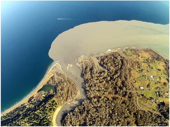
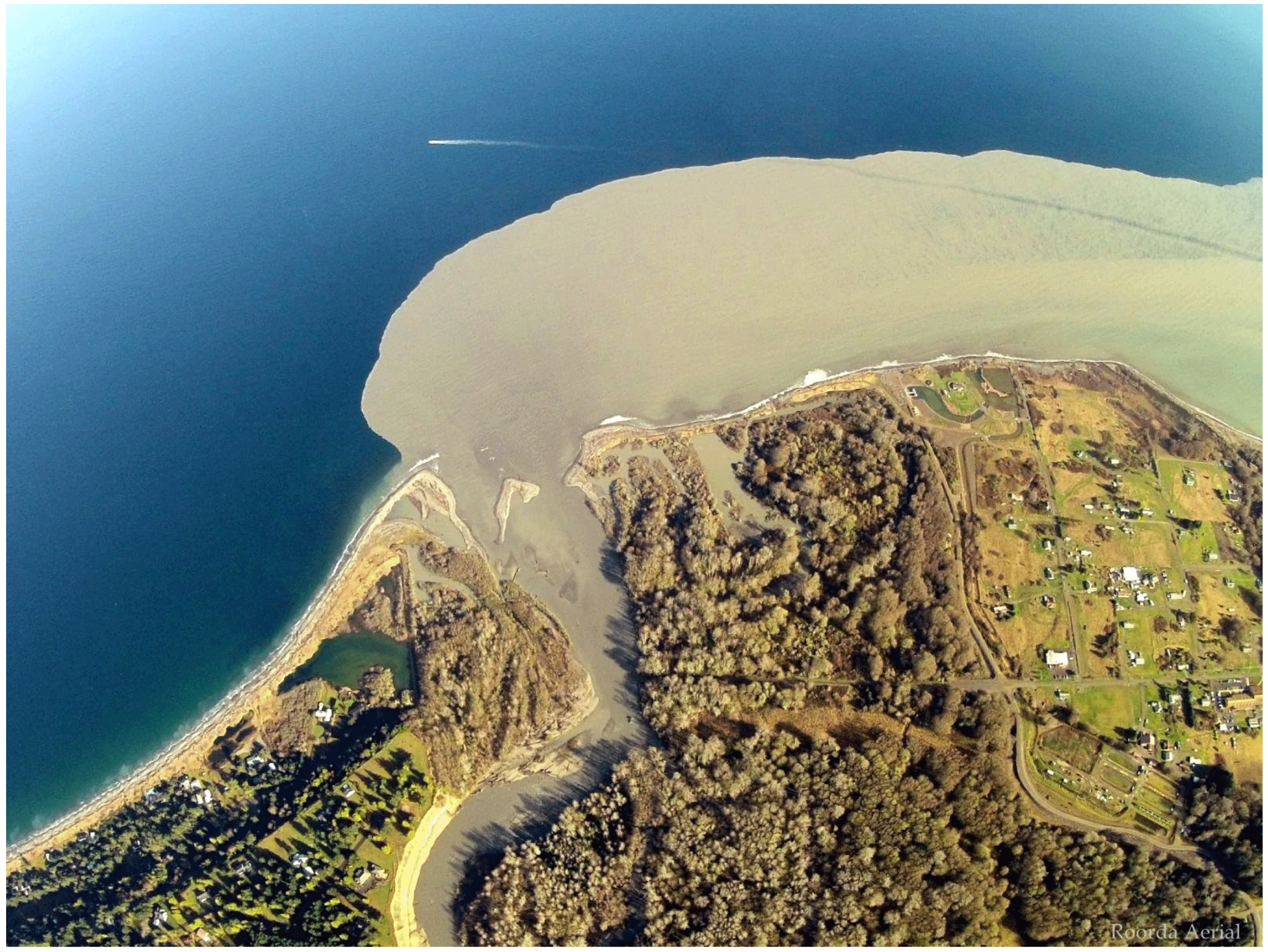
The flow of river water into the ocean transports nutrients, sediment and pollutants from the land to the sea, and as such the dynamics of coastal outflows is an active area of study. Field observations have revealed a rich variety of behaviours, with qualitative differences not only between different rivers but also at the same site during different seasons (Shetye et al. Reference Shetye, Gouveia, Shenoi, Sundar, Michael and Nampoothiri1993). It is often the case that outflows drive a coastally trapped current of fresh water along the right-hand shoreline (in the Northern Hemisphere) following the direction of Kelvin-wave propagation (Simpson & Hill Reference Simpson and Hill1986; Münchow & Garvine Reference Münchow and Garvine1993). A particularly striking case of this rightward flow occurred when a hydroelectric dam was removed from the Elwha river (Washington, USA) in 2014, releasing a large amount of silt that was clearly visible in aerial photographs (see figure 1). On the other hand, it is known that the Chang Jiang (Yangtze) river leaves a large deposit of brackish water to the left of the river mouth (Wensu Reference Wensu1988), while Shetye et al. (Reference Shetye, Gouveia, Shenoi, Sundar, Michael and Nampoothiri1993) identify a coastal trapped current in the Bay of Bengal that flows leftward for part of the year. Laboratory studies of buoyant outflows also observe anticyclonic gyres (or ‘bulges’) that trap fresh water near the source region (Avicola & Huq Reference Avicola and Huq2003; Horner-Devine et al. Reference Horner-Devine, Fong, Monismith and Maxworthy2006; Thomas & Linden Reference Thomas and Linden2007). This complexity and variation is due to the plethora of influencing factors (buoyancy, rotation, local geography, tidal currents) and highlights the importance of theoretical or numerical studies that seek to isolate the contribution made by each of these.
A hydroelectric dam on the Elwha river was removed in 2014, releasing a large build-up of silt into the Strait of Juan de Fuca. Image reproduced by permission of Tom Roorda.
Garvine (Reference Garvine1995) presents a complete classification of river outflows based on a scaling analysis. They identify the Kelvin number
 $K$
, the ratio of the current width to the Rossby radius
 $L_{R}$
, as the most important parameter, and categorise 12 sets of observational data based on estimates for
 $K$
. Outflows with small
 $K$
are expected to exhibit strong nonlinear behaviour including internal hydraulic jumps, and form radially symmetric bulges around the source mouth. They are thus little affected by rotation, and are found to occur in industrial discharges and narrow rivers. Large-scale discharges (
 $K\gg 1$
) have relatively slow flow and are in geostrophic balance. In the analysis below the current width is scaled on
 $L_{R}$
, placing the outflow in the intermediate
 $K=O(1)$
regime – although Garvine describes examples that exhibit large-scale behaviour when
 $K$
is as low as 2.
Several models have been used to understand the differences in outflow behaviours. McCreary, Zhang & Shetye (Reference McCreary, Zhang and Shetye1997) integrate a
 $1{\textstyle \frac{1}{2}}$
layer model with variable density and horizontal mixing of fresh and salty water, obtaining different qualitative behaviours depending on the Rossby number and total river transport. In particular, they find that all water bends to the left or flows directly offshore immediately after leaving the river mouth, and that only a portion of the total outflow recirculates to eventually propagate rightwards (hereafter, the direction of Kelvin-wave propagation in the Northern Hemisphere identifies ‘rightwards’ with downstream). The initial upstream flow (which they note is more prominent in their results than in real oceans) is driven by the geostrophic adjustment of buoyant water.
Both Kubokawa (Reference Kubokawa1991) and Johnson, Southwick & McDonald (Reference Johnson, Southwick and McDonald2017) (JSM hereafter) consider the effects of potential vorticity anomaly (PVa) on the river outflow by using a model in which the river water has the same density as a buoyant upper layer of oceanic fluid. If disturbances to the layer interface are small relative to the total depth of the layer, the problem can be formulated in terms of the quasi-geostrophic equations. If all fluid is stationary initially, and the source is impulsively switched on at
 $t=0$
, one can interpret this quasi-geostrophic limit as requiring an asymptotically small difference between the depth of the river mouth and the depth of the buoyant upper layer. In Kubokawa (Reference Kubokawa1991), the outflow is split between fluids of two different PVs. Part of the outflow has the same PV as the upper oceanic layer, and the remainder has a lower PV. Possible flows are split into three distinct classes depending on the total volume and PV distribution of the outflow, these being a steady coastal current, a widening current and an anticyclonic gyre mode. The river outflow in JSM is of uniform PV, and solutions are found to depend on the sign of the PV anomaly (PVa, the difference between the river PV and the PV of the buoyant ocean layer). Using numerical simulations (as well as analytic results when a long-wave assumption is imposed in addition to quasi-geostrophy) they find that all the river water travels downstream when the oceanic layer is deeper than the source (positive PVa, vortex stretching) while fluid travels in both directions if the oceanic layer is shallower than the source (negative PVa, vortex squashing). This identifies two mechanisms that drive the flow: flow driven downstream by a Kelvin wave and flow driven by image vorticity. The vortical flow is caused by the PV jump and, depending on the sign of the PVa, can drive fluid in either direction. In fact Johnson & McDonald (Reference Johnson and McDonald2006) showed that if the flow is completely dominated by image vorticity, it is possible to send all the expelled fluid to the left. In this limiting case, the vortical current has width
 $L_{v}=(Q_{0}/|\unicode[STIX]{x1D6F1}_{0}|H_{s})^{1/2}$
, where
 $Q_{0}$
is the total flux from the source,
 $\unicode[STIX]{x1D6F1}_{0}$
is the PVa and
 $H_{s}$
is the depth of the source.
Here, we present work that extends the uniform PV model of JSM by considering situations where the quasi-geostrophic approximation is no longer valid. That is, the difference between the initial upper-layer depth and the PV depth of the river water can be of arbitrary magnitude. Theoretical progress relies on invoking a long-wave assumption – that variations in the along-shore direction occur over a larger scale than those in the off-shore direction. This results in a semi-geostrophic (alongshore only) set of equations, which have been used previously for studying similar problems involving uniform PV, including hydraulic problems (Gill Reference Gill1977) and coastal currents (Stern Reference Stern1980; Stern, Whitehead & Hua Reference Stern, Whitehead and Hua1982; Kubokawa & Hanawa Reference Kubokawa and Hanawa1984a
; Stern & Helfrich Reference Stern and Helfrich2002). The boundary of these currents can be completely described by similarity solutions that relate the current width to the velocity at the current edge. Similar ideas are applicable for the present set-up, in regimes where the flow evolves to become steady. These steady flows can be matched with unsteady coastal currents away from the source region, and thus it is possible to develop a full theory for the flow behaviour that depends only on the non-dimensional mass flux
 $Q_{0}$
and the outer-layer depth
 $H$
.
The model developed below is probably too simple to make quantitative comparisons with data from real coastal outflows. In particular, it ignores density differences between the river water and the active ambient fluid. The model is designed to highlight the interaction between Kelvin-wave flow and vorticity dynamics, and direct application to the outflow problem is most appropriate in cases where these are the dominant dynamical features or in flows where entrainment is confined to the head of the current, as in the (non-rotating) experiments of Sher & Woods (Reference Sher and Woods2017).
Section 2 briefly derives the semi-geostrophic model from the rotating shallow-water equations. Section 3 gives numerical results and a complete theory for positive PVa. Section 4 presents numerical and theoretical results for negative PVa, and § 5 gives a brief comparison to oceanographic observations and laboratory experiments, as well as further discussion of the limitations of the model.
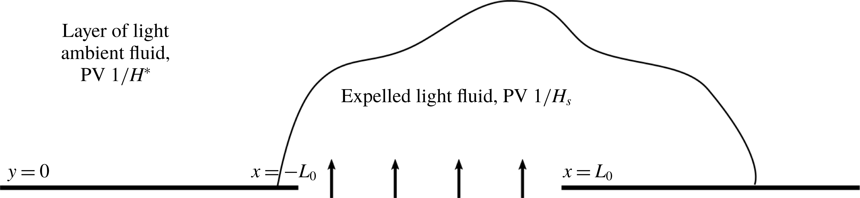
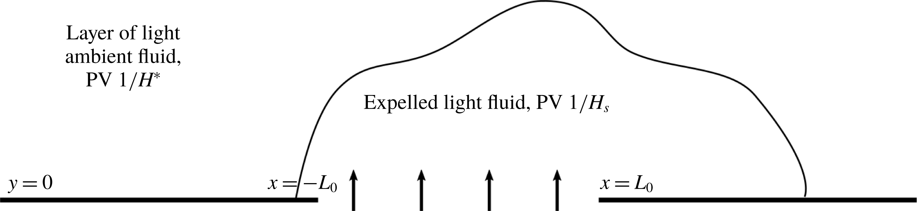
Fluid is expelled from a coastal source of depth
 $H_{s}$
located at
 $|x|<L_{0}$
,
 $y=0$
. The oceanic fluid in
 $y>0$
initially consists of a lighter layer (with the same density as the expelled fluid) of dimensional depth
 $H^{\ast }$
lying over a deep, denser, inactive layer.
2 Semi-geostrophic theory
Consider a layer of buoyant fluid with dimensional depth
 $H^{\ast }$
lying above an infinitely deep, inactive layer, with the whole system rotating about a vertical axis
 $Oz$
at constant angular speed
 $f/2>0$
, where
 $Oxyz$
are Cartesian axes fixed in the fluid. The fluid lies in
 $y>0$
, with the coast at
 $y=0$
a solid vertical boundary. At time
 $t=0$
, a coastal source lying between
 $-L_{0}<x<L_{0}$
is switched on. The fluid expelled by the source is of the same density of the active layer, but has a different PV. A schematic of this set-up is shown in figure 2. The active layer is taken to be sufficiently shallow to be governed by the reduced-gravity rotating shallow-water equations, which in non-dimensional form are
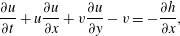 $$\begin{eqnarray}\displaystyle & \displaystyle \frac{\unicode[STIX]{x2202}u}{\unicode[STIX]{x2202}t}+u\frac{\unicode[STIX]{x2202}u}{\unicode[STIX]{x2202}x}+v\frac{\unicode[STIX]{x2202}u}{\unicode[STIX]{x2202}y}-v=-\frac{\unicode[STIX]{x2202}h}{\unicode[STIX]{x2202}x}, & \displaystyle\end{eqnarray}$$
 $$\begin{eqnarray}\displaystyle & \displaystyle \left(\frac{L_{R}}{L_{0}}\right)^{2}\left(\frac{\unicode[STIX]{x2202}v}{\unicode[STIX]{x2202}t}+u\frac{\unicode[STIX]{x2202}v}{\unicode[STIX]{x2202}x}+v\frac{\unicode[STIX]{x2202}v}{\unicode[STIX]{x2202}y}\right)+u=-\frac{\unicode[STIX]{x2202}h}{\unicode[STIX]{x2202}y}, & \displaystyle\end{eqnarray}$$
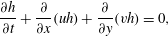 $$\begin{eqnarray}\displaystyle & \displaystyle \frac{\unicode[STIX]{x2202}h}{\unicode[STIX]{x2202}t}+\frac{\unicode[STIX]{x2202}}{\unicode[STIX]{x2202}x}(uh)+\frac{\unicode[STIX]{x2202}}{\unicode[STIX]{x2202}y}(vh)=0, & \displaystyle\end{eqnarray}$$
where
 $h$
is the depth of the active layer, and
 $u$
and
 $v$
are the along-shore and off-shore velocities respectively. Here
 $x$
has been non-dimensionalised with
 $L_{0}$
(so that the source lies in
 $|x|<1$
),
 $y$
with the Rossby radius for the source fluid
 $L_{R}=\sqrt{g^{\prime }H_{s}}/f$
, velocities
 $u$
and
 $v$
with
 $\sqrt{g^{\prime }H_{s}}$
and
 $\sqrt{g^{\prime }H_{s}}(L_{R}/L_{0})$
respectively,
 $h$
with
 $H_{s}$
(the source depth) and
 $t$
with the advective time scale
 $L_{0}/\sqrt{g^{\prime }H_{s}}$
, where
 $g^{\prime }$
is the reduced gravity for the upper layer.
Taking the limit
 $L_{R}/L_{0}\rightarrow 0$
gives the semi-geostrophic or long-wave equations, and requires that the flow is slowly varying in the
 $x$
direction, or that the river mouth is wide relative to the Rossby radius. The semi-geostrophic equations can in fact still be valid when variations in
 $x$
are fast (for example, in the region of a shock) provided the off-shore velocity
 $v\ll u$
(Kubokawa & Hanawa Reference Kubokawa and Hanawa1984b
). The long-wave assumption requires further justification in the source region, especially at early times when
 $v$
and
 $u$
are of the same order, and the
 $x$
and
 $y$
scales are similar. Strong support for the use of this scaling comes from JSM, where they find excellent agreement between their long-wave theory and contour-dynamic simulations of the full quasi-geostrophic (QG) problem, even in simulations where fluid is expelled from a point source (their figures 11–13). Discrepancies do exist in the source region, but it appears that the long-wave scaling does not affect the qualitative behaviour of the outflow, including the strength of the upstream propagation in outflows with negative PVa.
A standard manipulation of (2.1)–(2.3) shows that the PV
 $$\begin{eqnarray}q=\frac{1-\unicode[STIX]{x2202}u/\unicode[STIX]{x2202}y+(L_{R}/L_{0})^{2}\unicode[STIX]{x2202}v/\unicode[STIX]{x2202}x}{h}\end{eqnarray}$$
is conserved by fluid parcels (Stern Reference Stern1980). Taking the limit
 $L_{R}/L_{0}\rightarrow 0$
and substituting (2.2) gives the field equation for
 $h$
,
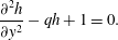 $$\begin{eqnarray}\frac{\unicode[STIX]{x2202}^{2}h}{\unicode[STIX]{x2202}y^{2}}-qh+1=0.\end{eqnarray}$$
The ambient outer layer begins at rest with non-dimensional depth
 $H$
and so has PV
 $q_{out}=1/H$
and, by scaling
 $h$
with the depth of the river mouth
 $H_{s}$
, the expelled fluid has PV
 $q_{in}=1$
. Thus
 $H>1$
corresponds to positive PVa, and
 $H<1$
to negative PVa. In the scenario described here, where a source of uniform depth is turned on at
 $t=0$
, the choice of uniform PV would seem to be completely natural. This restriction on the river mouth geometry is not necessary for the outflow to have uniform PV. One could instead consider flow from a wide, deep upstream reservoir as in Gill (Reference Gill1977), where
 $H_{s}$
is the potential vorticity depth of the river water. In either case, the use of piecewise-constant PV is a necessary simplification required to solve (2.5) and make analytical progress. Although real outflows probably have non-constant PV, uniform models have been used to provide a theoretical framework for understanding large-scale ocean flows (Stern Reference Stern1980; Kubokawa Reference Kubokawa1991; Helfrich, Kuo & Pratt Reference Helfrich, Kuo and Pratt1999, for example) and this simplification has also been used successfully to describe laboratory experiments that simulate coastal outflows (Thomas & Linden Reference Thomas and Linden2007; Gregorio et al.
Reference Gregorio, Haidvogel, Thomas, Taskinoglu and Skeen2011).
The Rossby number of the flow can be defined, following Clarke & Johnson (Reference Clarke and Johnson1999), as
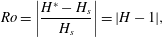 $$\begin{eqnarray}Ro=\left|\frac{H^{\ast }-H_{s}}{H_{s}}\right|=|H-1|,\end{eqnarray}$$
that is, the ratio of the PVa and background PV. Note that this is also the fractional depth change between the outflow and the ambient layer, and thus the limit
 $Ro\rightarrow 0$
recovers quasi-geostrophic flow.
Provided it does not overturn, the boundary of the expelled fluid can be described as a single-valued function
 $y=w(x,t)$
and the field equation (2.5) can be solved separately in the river water and the ambient to obtain
 $$\begin{eqnarray}h=\left\{\begin{array}{@{}ll@{}}H+\sqrt{H}U\text{e}^{(w-y)/\surd H}\quad & y>w(x,t),\\ 1+(H-1+\sqrt{H}U)\cosh (w-y)+U\sinh (w-y)\quad & 0<y<w(x,t).\end{array}\right.\end{eqnarray}$$
The solutions (2.7) are constructed so that
 $h$
and
 $u$
are continuous at
 $y=w$
, which is equivalent to requiring a continuous pressure in the fluid and enforcing the kinematic boundary condition. The problem is now reduced to finding
 $w(x,t)$
, along with the speed at the current edge
 $U(x,t)=u(x,w,t)$
, from which the full velocity and depth profiles can be reconstructed.
Other quantities that appear in the calculations below are the layer depths at the wall and the current edge, and the fluid velocity at the wall. These are given by
 $$\begin{eqnarray}\displaystyle & \displaystyle h_{W}=h(x,0,t)=1+(H-1+\sqrt{H}U)\cosh (w)+U\sinh (w), & \displaystyle\end{eqnarray}$$
 $$\begin{eqnarray}\displaystyle & \displaystyle h_{e}=h(x,w,t)=H+\sqrt{H}U, & \displaystyle\end{eqnarray}$$
 $$\begin{eqnarray}\displaystyle & \displaystyle u_{W}=u(x,0,t)=U\cosh (w)+(H+\sqrt{H}U-1)\sinh (w). & \displaystyle\end{eqnarray}$$
The mass flux of oceanic fluid at a station
 $x$
is given by
 $$\begin{eqnarray}\int _{w}^{\infty }uh\,\text{d}y=\left.\frac{h^{2}}{2}\right|_{\infty }^{w}=\frac{h_{e}^{2}}{2}-\frac{H^{2}}{2},\end{eqnarray}$$
so that the flux of ocean fluid is downstream only if
 $h_{e}>H$
which, by (2.9), is only true if
 $U>0$
. It is shown below that all outflows have
 $U\geqslant 0$
, and so if there is net transport of oceanic fluid this is always from upstream of the source to downstream. Along with (2.7), this also implies that all currents in the oceanic fluid are unidirectional.
Stern (Reference Stern1980) notes that, from (2.3), the
 $y$
-derivative of the alongshore momentum equation (2.1) vanishes, and so the latter needs to be satisfied at one
 $y$
-value only. For the outflow problem here,
 $U$
and
 $w$
can thus be found by solving (2.1) at the current edge subject to an integrated form of mass conservation (2.3), i.e.
 $$\begin{eqnarray}\displaystyle & \displaystyle \frac{\unicode[STIX]{x2202}U}{\unicode[STIX]{x2202}t}+U\frac{\unicode[STIX]{x2202}U}{\unicode[STIX]{x2202}x}+\sqrt{H}\frac{\unicode[STIX]{x2202}U}{\unicode[STIX]{x2202}x}-\frac{\unicode[STIX]{x2202}w}{\unicode[STIX]{x2202}t}=0, & \displaystyle\end{eqnarray}$$
 $$\begin{eqnarray}\displaystyle & \displaystyle \frac{\unicode[STIX]{x2202}}{\unicode[STIX]{x2202}t}\int _{0}^{w}h\,\text{d}y+H\left(\frac{\unicode[STIX]{x2202}U}{\unicode[STIX]{x2202}t}-\frac{\unicode[STIX]{x2202}w}{\unicode[STIX]{x2202}t}\right)+h_{W}\frac{\unicode[STIX]{x2202}h_{W}}{\unicode[STIX]{x2202}x}=Q^{\prime }(x), & \displaystyle\end{eqnarray}$$
where
 $$\begin{eqnarray}\int _{0}^{w}h\,\text{d}y=(H-1)\sinh (w)+w+U(-1+\cosh (w)+\sqrt{H}\sinh (w)).\end{eqnarray}$$
Here,
 $Q(x)$
is a monotonic-increasing function that gives the (steady) cumulative volume flux from the river mouth for
 $t>0$
through
 $$\begin{eqnarray}\int _{-1}^{x}vh|_{y=0}\,\text{d}x^{\prime }=Q(x)\end{eqnarray}$$
so that the total mass flux from the source is
 $Q_{0}=Q(1)$
which, along with
 $H$
, is a key physical parameter for the flow. The no-flux boundary condition at the coast can be applied by extending
 $Q(x)$
to take values zero and
 $Q_{0}$
in
 $x<-1$
and
 $x>1$
respectively. The long-term evolution of the current away from the source region is found below to depend on
 $Q(x)$
only through the total mass flux
 $Q_{0}$
, and so for simplicity all examples presented here use the linear profile
 $Q(x)=(Q_{0}/2)(x+1)$
in
 $|x|<1$
. The theory below classifies the qualitative behaviour of the outflow in terms of the two parameters
 $Q_{0}$
and
 $H$
, and so applies to any steady volume-flux profile
 $Q(x)$
, including those resulting from a critically controlled outflow. Results presented here can also be easily extended to unsteady outflows, and an analysis of such changes is explored in more detail for the quasi-geostrophic limit in Southwick, Johnson & McDonald (Reference Southwick, Johnson and McDonald2017).
2.1 Constants of motion
Benjamin & Lighthill (Reference Benjamin and Lighthill1954) describe trains of steadily translating long gravity waves using three constants of motion: volume flux, alongshore momentum flux and total energy. The volume flux of river water is simply the parameter
 $Q_{0}$
, and similar expressions for the momentum flux and total energy can also be derived.
Multiplying the
 $x$
-momentum equation (2.1) by
 $h$
, the mass conservation equation (2.3) by
 $u$
, taking the sum of these and integrating from
 $y=0$
to
 $y=\infty$
gives
 $$\begin{eqnarray}\frac{\unicode[STIX]{x2202}}{\unicode[STIX]{x2202}t}\int _{0}^{\infty }uh\,\text{d}y+\frac{\unicode[STIX]{x2202}}{\unicode[STIX]{x2202}x}\int _{0}^{\infty }\left(hu^{2}+\frac{h^{2}}{2}\right)\text{d}y-u_{W}h_{W}v_{W}=\int _{0}^{\infty }vh\,\text{d}y.\end{eqnarray}$$
(Note that these terms are bounded because the fluid is stagnant as
 $y\rightarrow \infty$
.) The right-hand side of (2.16) can be computed by multiplying (2.3) by
 $y$
and integrating,
 $$\begin{eqnarray}\int _{0}^{\infty }vh\,\text{d}y=\frac{\unicode[STIX]{x2202}}{\unicode[STIX]{x2202}t}\int _{0}^{\infty }yh\,\text{d}y+\frac{\unicode[STIX]{x2202}}{\unicode[STIX]{x2202}x}\int _{0}^{\infty }yuh\,\text{d}y,\end{eqnarray}$$
so that (2.16) becomes
 $$\begin{eqnarray}\frac{\unicode[STIX]{x2202}I}{\unicode[STIX]{x2202}t}+\frac{\unicode[STIX]{x2202}S}{\unicode[STIX]{x2202}x}=u_{W}h_{W}v_{W},\end{eqnarray}$$
where
 $$\begin{eqnarray}I=\int _{0}^{\infty }(u-y)h\,\text{d}y,\quad S=\int _{0}^{\infty }\left(hu(u-y)+\frac{h^{2}}{2}\right)\,\text{d}y\end{eqnarray}$$
are the along-wall impulse and the flow force respectively. The quantity
 $u_{W}h_{W}v_{W}$
is the downstream momentum input at the wall, and vanishes away from the source region. The total downstream momentum added across the source in steady flow is thus
 $$\begin{eqnarray}S_{0}=\int _{-1}^{1}u_{W}Q^{\prime }(x)\,\text{d}x=\int _{0}^{Q_{0}}u_{W}\,\text{d}Q,\end{eqnarray}$$
giving a second constant of the motion. The momentum input term is discussed in greater detail for QG flow in Southwick et al. (Reference Southwick, Johnson and McDonald2017), where its presence is shown to resolve the momentum imbalance paradox of Pichevin & Nof (Reference Pichevin and Nof1997).
In steady flow, (2.3) allows a volume-flux streamfunction
 $\unicode[STIX]{x1D713}$
to be defined such that
 $vh=\unicode[STIX]{x1D713}_{x}$
and
 $uh=-\unicode[STIX]{x1D713}_{y}$
. The
 $x$
-momentum equation (2.1) can be integrated once in
 $x$
to give
 $$\begin{eqnarray}\frac{u^{2}}{2}-\unicode[STIX]{x1D713}+h=R.\end{eqnarray}$$
Since the
 $y$
-derivative of (2.1) vanishes,
 $R$
is constant throughout the flow, providing a third constant of motion for steady flow that can be found by evaluating (2.21) at the wall, where
 $\unicode[STIX]{x1D713}=Q$
.
2.2 Vortical and Kelvin-wave-driven flow
There are two principal mechanisms that drive the outflow, and it is instructive to see how their relative strengths affect the behaviour of solutions.
The first of these mechanisms is flow driven by a Kelvin wave, which propagates faster than the river water and thus transports both river and oceanic fluid (Helfrich et al.
Reference Helfrich, Kuo and Pratt1999; Helfrich Reference Helfrich2006). To isolate the effects of this wave, consider the zero-PVa problem (that is, with
 $H=1$
). The expression for the layer depth is now
 $$\begin{eqnarray}h=1+B(x,t)\text{e}^{-y}\end{eqnarray}$$
where
 $B$
satisfies the
 $x$
-momentum equation (2.1) at the wall,
 $$\begin{eqnarray}\frac{\unicode[STIX]{x2202}B}{\unicode[STIX]{x2202}t}+(1+B)\frac{\unicode[STIX]{x2202}B}{\unicode[STIX]{x2202}x}=Q^{\prime }(x).\end{eqnarray}$$
This is the forced Hopf equation, which can be solved explicitly using the method of characteristics, and gives rise to a current that expands offshore and heads downstream, moving with speed
 $u_{KW}=-1+\surd (1+2Q_{0})$
at the wall. This is referred to hereafter as the Kelvin-wave flow. Non-trivial solutions of the homogeneous Hopf equation always develop shocks, which occur in the present problem in the oceanic (rather than river) water at the leading edge of the Kelvin-wave flow. These shocks are discussed in greater detail in § 3.5.
The other effect that drives the flow is image vorticity. Vortical columns expelled by the source stretch or squash as they adjust to match the depth of the oceanic layer, and this drives a change in relative vorticity, which in turn acts to send fluid downstream (vortex stretching, positive PVa) or upstream (vortex squashing, negative PVa). This effect can be isolated by considering the limiting case of rotating fluid ejected into a non-rotating background, and it is shown in Johnson & McDonald (Reference Johnson and McDonald2006) that the velocity of the current at the wall is
 $u_{V}=\pm \surd (Q_{0}|H-1|/H)$
where the sign depends on the sign of the PVa. Thus, for positive PVa both the vortical and Kelvin-wave effects drive fluid downstream, while for negative PVa the two effects are in opposition.
The relative strengths of these two effects can be measured by the ratio between the two speeds:
 $$\begin{eqnarray}a=\frac{|u_{V}|}{u_{KW}}=\frac{\sqrt{Q_{0}|H-1|}}{-\surd H+\surd H(1+2Q_{0})}.\end{eqnarray}$$
When the jump in PV is small, and the flow is quasi-geostrophic, JSM found that solutions can be fully characterised by the value of
 $a$
and the sign of the PVa, and one of the main goals of the present work is to assess to what extent
 $a$
can be used to categorise solutions to the semi-geostrophic problem at larger values of
 $Ro$
. It is expected, and shown below, that the results here reduce to those of JSM in the limit
 $Ro\rightarrow 0$
and
 $Q_{0}\rightarrow 0$
, with
 $a\sim \surd (Ro/Q_{0})$
fixed. In this limit,
 $a$
can also be identified as the ratio of the Rossby radius
 $L_{R}$
to the vortical width
 $L_{V}=\surd (Q_{0}H/|H-1|)$
(the width of the vortical current). The two interpretations are interchangeable in the quasi-geostrophic limit, but for
 $Ro=O(1)$
the definition (2.24) in terms of speed is more instructive.
Note that the choice of
 $L_{R}$
for horizontal length scales ensures that the length over which the Kelvin wave decays is
 $O(1)$
, while vortical currents can be of arbitrary width. On the other hand, JSM scale horizontal lengths on
 $L_{V}$
, thus keeping the vortical current width at
 $O(1)$
and allowing the Kelvin-wave decay scale to be arbitrarily small as
 $a\rightarrow 0$
. Anticipating the importance of
 $a$
in determining the behaviour of the flow, we will briefly outline some results from the quasi-geostrophic limit.
When
 $a<1$
, the Kelvin-wave-driven flow is dominant:
 $|u_{V}|<u_{KW}$
and
 $L_{R}<L_{V}$
. For positive PVa, the Kelvin wave pulls ahead of the vortical flow, vortical turning is weak at the nose of the fluid and the outflow boundary joins smoothly to the coast. Depth perturbations decay quickly away from the wall before vortical effects can take hold. For negative PVa, the weak vortical flow is not sufficient to counteract the Kelvin wave, and the solution expands indefinitely away from the coast, with fluid spreading up and downstream.
When
 $a>1$
, vorticity dynamics dominate the outflow:
 $|u_{V}|>u_{KW}$
and
 $L_{R}>L_{V}$
. For positive PVa, vortex turning affects fluid closer to the wall, causing the current to overturn and a shock to form. As
 $a$
increases further, this happens over a shorter and shorter scale until, for
 $a=a_{m}\approx 1.868$
, the vortical current manages to adjust to the far-field condition within the expelled fluid and there is no disturbance in the oceanic fluid
 $y>w$
. In this case, the solution downstream is a current of constant width and no transport around the edge. For negative PVa, the relatively stronger vortical flow balances the Kelvin wave and the flow is steady in the source region.
3 Outflows with positive PVa
3.1 Numerical results
Having now reduced the problem to two nonlinear partial differential equations (2.12) and (2.13) in
 $x$
and
 $t$
, solutions can be obtained numerically. Starting from the initial conditions
 $U=w=0$
, the equations are integrated away from
 $t=0$
using the Lax–Wendroff method with a nonlinear smoothing filter (Engquist, Lötstedt & Sjögreen Reference Engquist, Lötstedt and Sjögreen1989) to prevent overshoot in the region of a shock. To ensure that the numerical scheme explicitly preserves mass and momentum, the equations are solved in conservation form, i.e.
 $$\begin{eqnarray}\frac{\unicode[STIX]{x2202}}{\unicode[STIX]{x2202}t}\left(\begin{array}{@{}c@{}}\unicode[STIX]{x1D719}_{1}\\ \unicode[STIX]{x1D719}_{2}\end{array}\right)+\frac{\unicode[STIX]{x2202}}{\unicode[STIX]{x2202}x}\left(\begin{array}{@{}c@{}}U^{2}/2+\sqrt{H}U\\ h_{W}^{2}/2\end{array}\right)=\left(\begin{array}{@{}c@{}}0\\ Q^{\prime }(x)\end{array}\right),\end{eqnarray}$$
where
 $$\begin{eqnarray}\unicode[STIX]{x1D719}_{1}=U-w,\quad \unicode[STIX]{x1D719}_{2}=\int _{0}^{w}h\,\text{d}y+H(U-w).\end{eqnarray}$$
This presents some difficulty, since the flux functions in (3.1) cannot be written explicitly in terms of
 $\unicode[STIX]{x1D719}_{1}$
and
 $\unicode[STIX]{x1D719}_{2}$
, and so
 $U$
and
 $w$
must be extracted at each grid point and each time step. This is done via Newton’s method, using as an initial guess the values of the solution at the previous time step. Applying homogenous Neumann boundary conditions at the upstream end of the spatial domain increases stability. Runs are conducted with grid spaces of
 $\unicode[STIX]{x0394}t=0.01$
or
 $0.005$
, and
 $\unicode[STIX]{x0394}x\approx 0.03$
as increasing the resolution further made no noticeable difference.
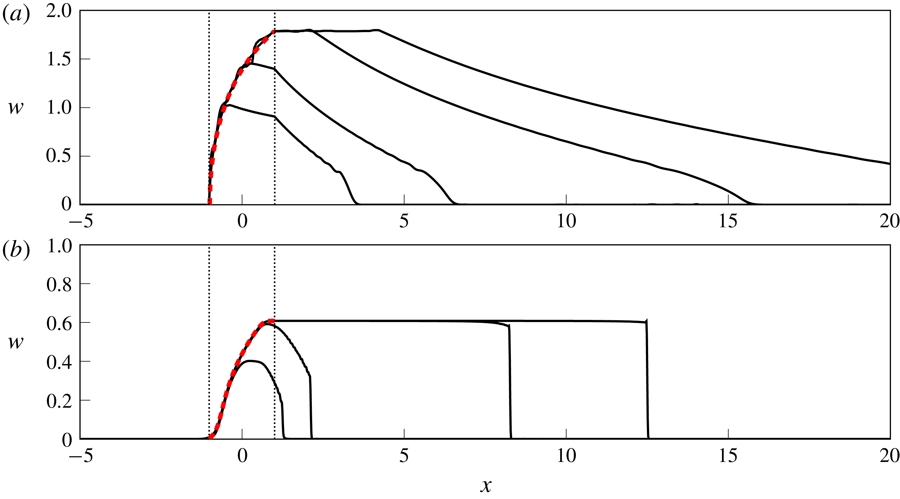
The off-shore extent of the expelled fluid,
 $y=w(x,t)$
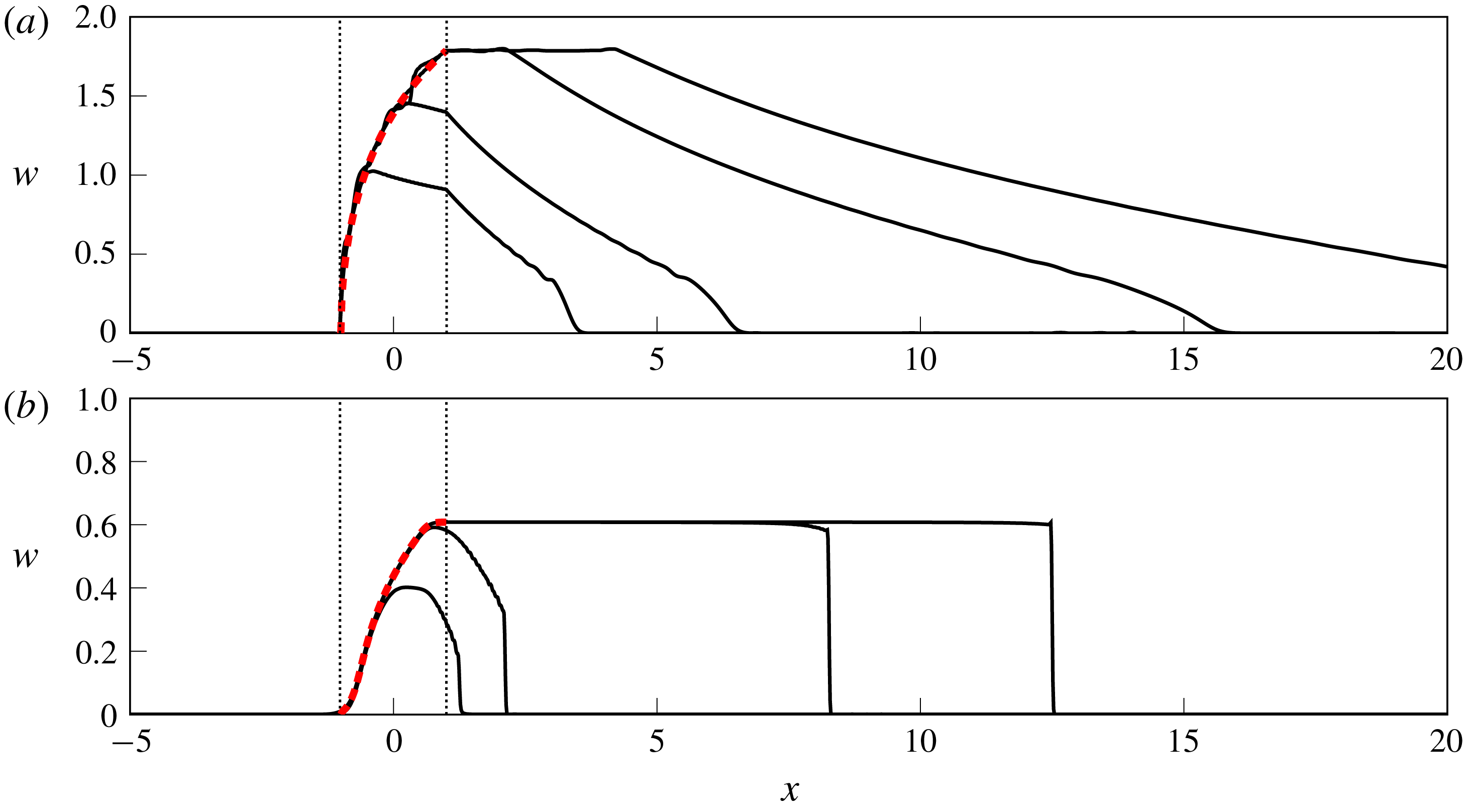
, for flows with positive PV anomaly. (a)
 $Q_{0}=1$
,
 $Ro=0.3$
and hence
 $a=0.66$
(Kelvin-wave-dominated flow) at
 $t=5,10,25,40$
. (b)
 $Q_{0}=0.4$
,
 $Ro=1$
and
 $a=1.31$
(vortically dominated flow) at
 $t=5,10,40,60$
. Vertical dotted lines mark the source region, and the dashed curve (red online) is the steady profile
 $w_{sp}$
computed in § 3.2.
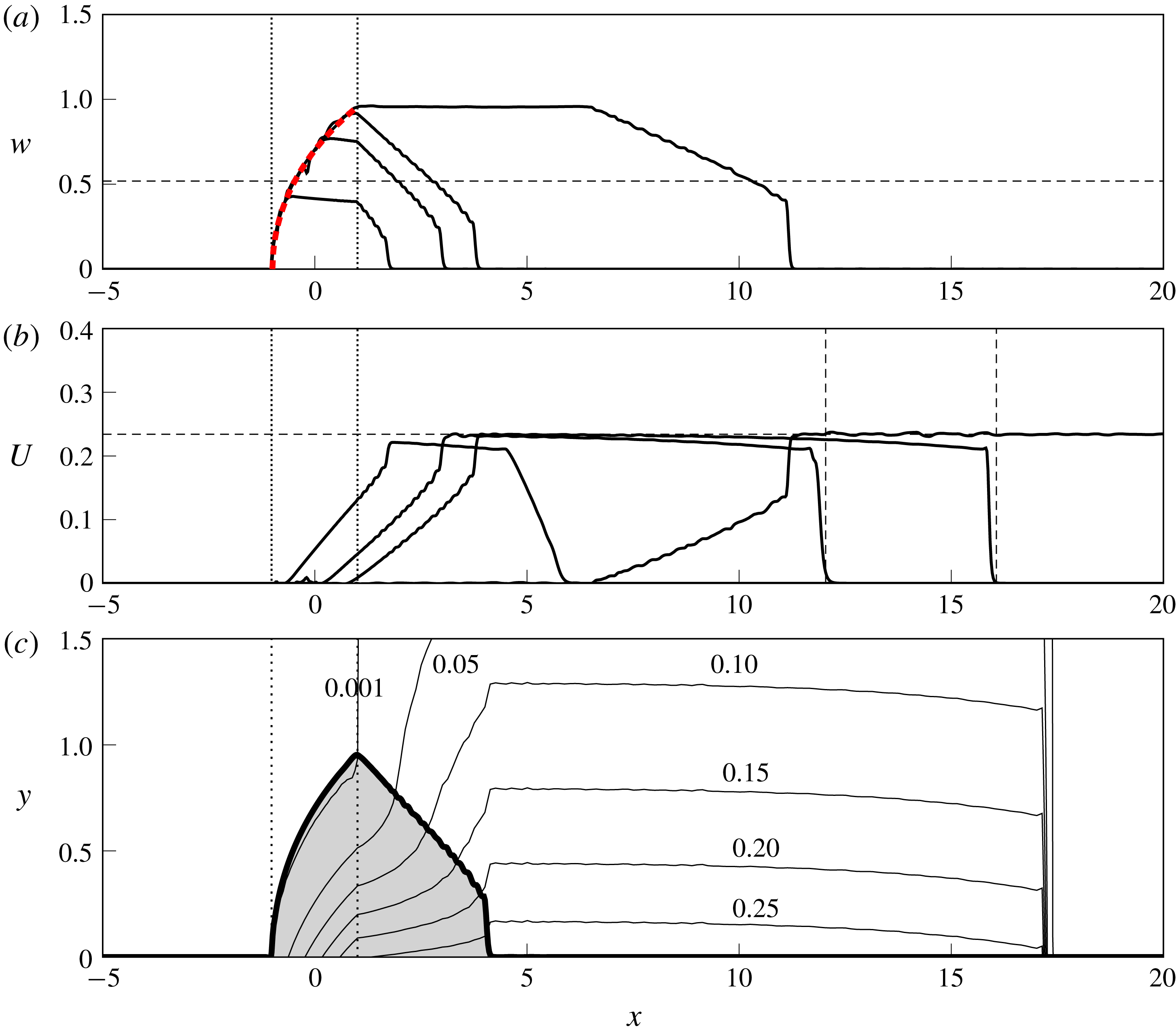
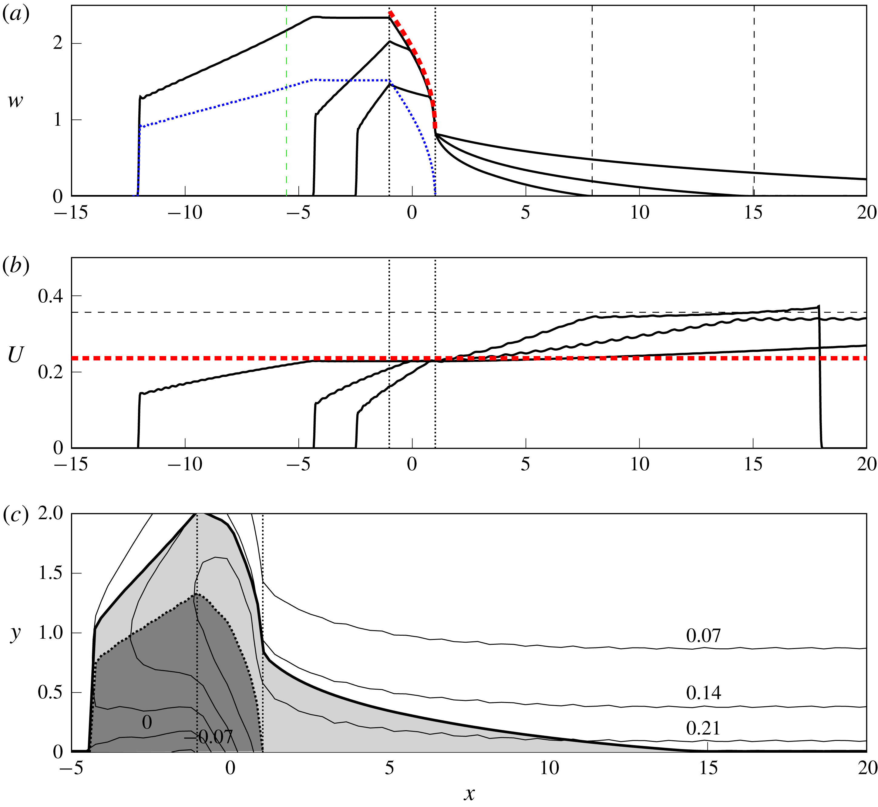
Outflow with positive PVa,
 $Q_{0}=0.4$
,
 $Ro=0.5$
and hence
 $a=1.07$
. (a) The current width
 $w$
and (b) the edge velocity
 $U$
are shown at times
 $t=4,9,12,40$
. The thick dashed curve (red online) in (a) gives the steady profile
 $w_{sp}$
, and thin dashed lines correspond to predictions from the theory of §§ 3.3–3.5. (c) Contours of
 $h-H$
, perturbations to the depth of the upper layer at
 $t=12$
. The thick curve gives
 $w$
at the same time, thus the shaded region is the extent of the expelled fluid.
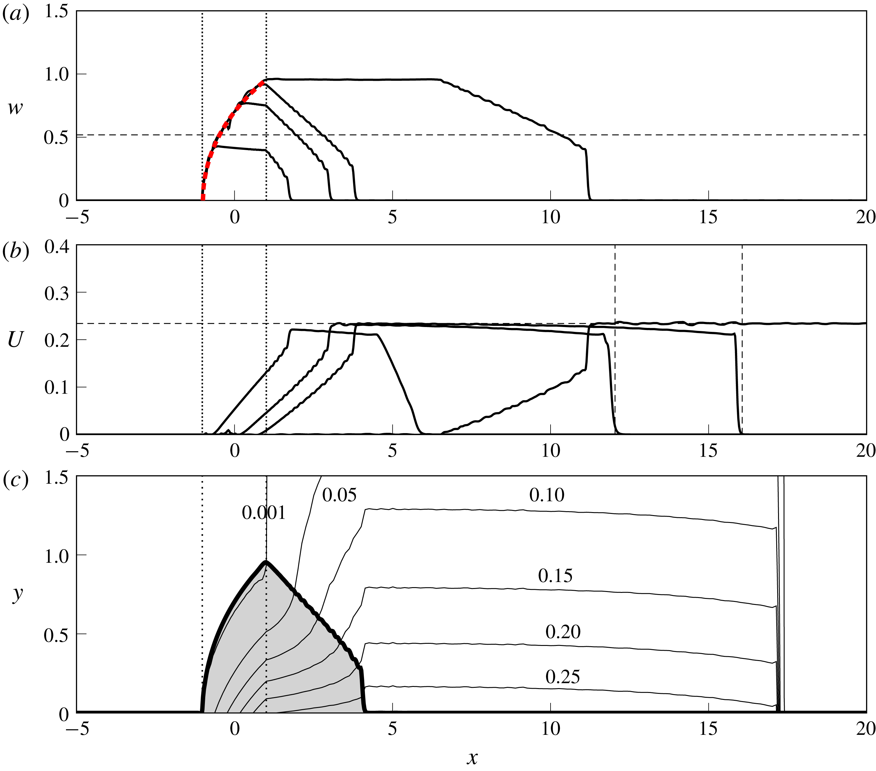
Figure 3 shows numerically computed
 $w$
for two different sets of parameters, with each panel showing the solution at several times. Figure 4 shows
 $w$
,
 $U$
and contours of
 $h-H$
for a third set of parameters. In all plots, the source region is marked by vertical dotted lines, and theoretical results derived below are shown by dashed lines. From the two functions
 $w$
and
 $U$
, the depth and velocity profile at any point can be computed using (2.7).
In all solutions with positive PVa, a steady current forms across the source region. This current width increases monotonically across the source, and the fluid at the current edge has zero velocity, so the outer layer is undisturbed in regions where the flow is steady. Numerical results agree excellently with the theory (heavy dashed curve, red online) presented in § 3.2. Once the steady solution reaches all the way across the source, a steady current of constant width propagates downstream.
Downstream of the steady region, the current narrows and the velocity around the edge increases according to a similarity solution discussed in § 3.3. The parameters are chosen to illustrate the range of possible behaviours and, as in JSM, these correlate with the value of the speed ratio
 $a$
. For small
 $a$
, as in figure 3(a), the flow is dominated by the Kelvin wave and the downstream current joins smoothly to the wall. For larger
 $a$
, as in figures 3(b) and 4(a), vorticity is stronger and the current terminates in a shock. The width of the shock increases monotonically, until it reaches a maximum value that is set by the flow parameters. If
 $a$
is large enough, and vortical effects are strongly dominant, this maximum value can be the same as the width of the steady current at the downstream edge of the source region, in which case there is no rarefaction and the solution after a finite time is a ‘blunt-headed current’ (cf. figure 3
b).
In regions where
 $w=0$
, the governing equations are still valid but
 $U$
is now to be interpreted as the velocity at the wall, and the layer depth decays exponentially away from the coast like
 $U\exp (-y/\surd H)$
. At all times and for all parameters, a nonlinear Kelvin wave propagates ahead of the expelled fluid. That is,
 $U>0$
in some region where
 $w=0$
. The effects of this are most clearly seen in the contour plot of figure 4(c): the river water (shaded) has reached
 $x=4$
, but the wall depth is increased by 0.25 over the region
 $4<x<16$
, an interfacial disturbance travelling in the oceanic fluid ahead of the river water. In the quasi-geostrophic limit, the Kelvin wave travels at infinite speed in the outer layer and so is not seen explicitly in the solutions – although it still induces a flow of finite velocity in the river water. Moving away from the quasi-geostrophic limit and permitting arbitrary values of
 $H$
changes the scale to one where the Kelvin wave is clearly visible, and information propagates at finite speed in both the river fluid and the oceanic layer. This Kelvin wave is discussed in detail in § 3.5.
3.2 Analysis across the source region
Since the PVa is positive, the image vorticity and the Kelvin wave both drive the flow downstream. System (2.12), (2.13) has two eigenvalues,
 $\unicode[STIX]{x1D706}_{R}$
and
 $\unicode[STIX]{x1D706}_{C}$
, with
 $\unicode[STIX]{x1D706}_{R}\leqslant \unicode[STIX]{x1D706}_{C}$
always (see appendix A for more details). Kubokawa & Hanawa (Reference Kubokawa and Hanawa1984a
) note that
 $\unicode[STIX]{x1D706}_{C}$
is a nonlinear coastal wave, and that
 $\unicode[STIX]{x1D706}_{R}$
is associated with disturbances at the current edge – across which the density jump from their model has been replaced by a PV jump in the present work.
When
 $w=U=0$
, one can show that
 $\unicode[STIX]{x1D706}_{R}=0$
and
 $\unicode[STIX]{x1D706}_{C}=\sqrt{H}$
. Thus, characteristics
 $\unicode[STIX]{x1D706}_{R}$
that start in
 $x<-1$
are unable to reach the source region. Further, it is impossible to satisfy
 $\unicode[STIX]{x1D706}_{C}=0$
or
 $\unicode[STIX]{x1D706}_{R}=0$
when
 $U>0$
and
 $H>1$
and so the flow is supercritical everywhere in
 $x>-1$
, with no information able to propagate upstream.
Since the characteristic speed
 $\unicode[STIX]{x1D706}_{R}$
vanishes at
 $x=-1$
and long-wave disturbances are stationary here, this is the control point for the steady flow that forms across the source region. The flow matches smoothly to the undisturbed outer layer at
 $x=-1$
, where
 $w=U=0$
.
Solving the steady versions of (2.12) and (2.13) gives
 $$\begin{eqnarray}\displaystyle & \displaystyle U=c_{1}, & \displaystyle\end{eqnarray}$$
 $$\begin{eqnarray}\displaystyle & \displaystyle h_{W}=\sqrt{2Q(x)+c_{2}}, & \displaystyle\end{eqnarray}$$
where
 $c_{1}$
and
 $c_{2}$
are constants of integration determined by the requirement that
 $U$
and
 $h_{W}$
are continuous at
 $x=-1$
to be 0 and
 $H^{2}$
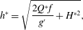
respectively. Downstream, the dimensional depth of the current at the wall is therefore
 $$\begin{eqnarray}h^{\ast }=\sqrt{\frac{2Q^{\ast }f}{g^{\prime }}+H^{\ast 2}},\end{eqnarray}$$
where
 $Q^{\ast }$
and
 $H^{\ast }$
are the (dimensional) mass flux and outer-layer depth respectively. The relationship (3.5) can be derived from a simple quasi-geostrophic scaling argument when
 $H=0$
(Chant Reference Chant, Wolanski and McLusky2011, p. 218).
Solving (2.8) for
 $w$
provides the steady solution
 $$\begin{eqnarray}w_{sp}(Q)=\operatorname{acosh}\left(\frac{\sqrt{2Q+H^{2}}-1}{H-1}\right),\end{eqnarray}$$
which is valid exactly when
 $H>1$
. The steady solution
 $w_{sp}$
is shown as a dashed curve (red online) in figures 3 and 4(a). Agreement with the numerical results is excellent in all cases. The steady current depends on
 $x$
only parametrically through
 $Q$
, and hence the downstream current width
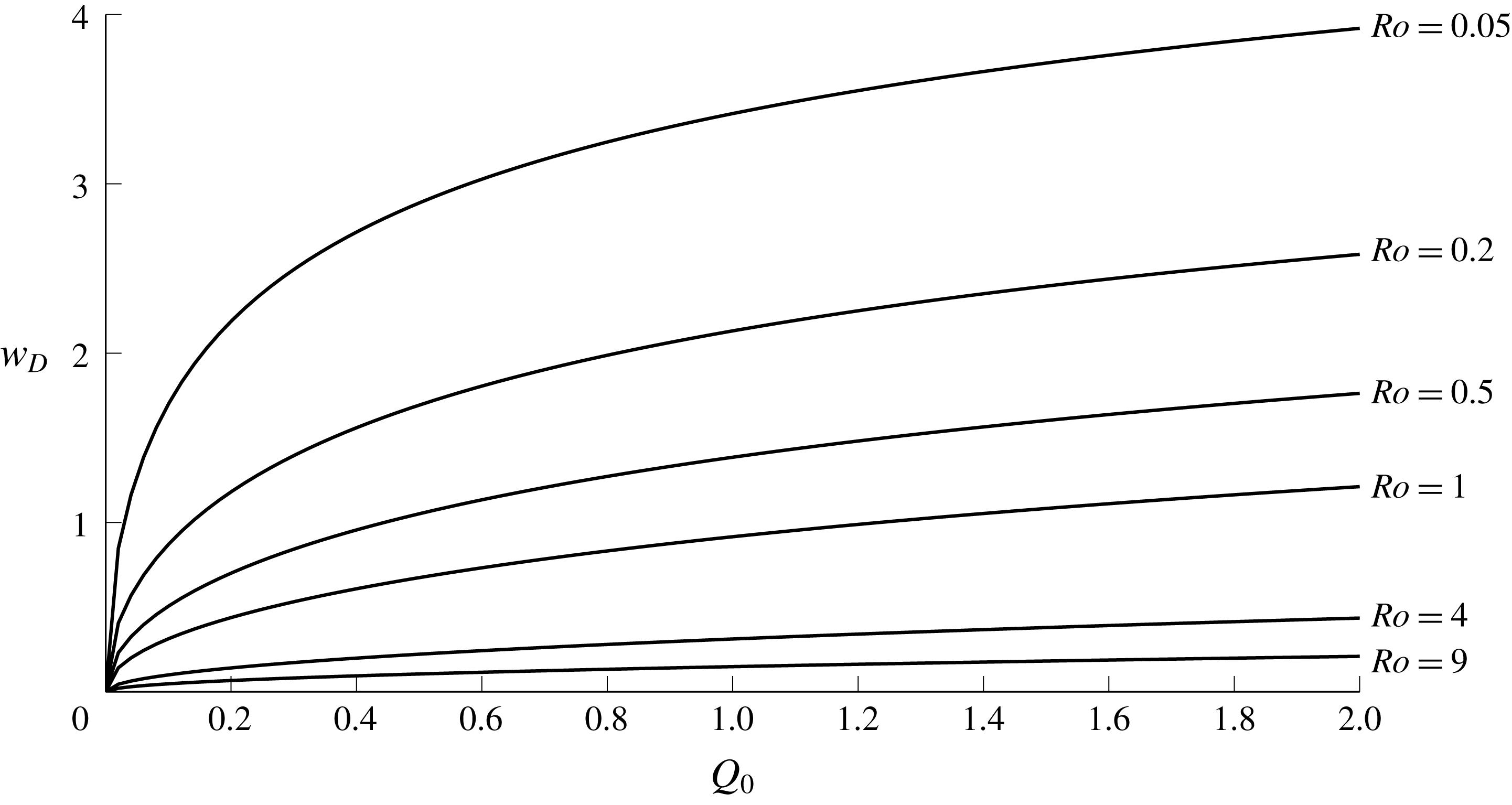
 $w_{D}=w_{sp}(Q_{0})$
does not depend on the specific form of the outflow velocity. In the quasi-geostrophic limit,
 $Ro\rightarrow 0$
and
 $Q_{0}\rightarrow 0$
with
 $a^{2}=Ro/Q_{0}$
fixed,
 $$\begin{eqnarray}w_{D}\sim \log (1+1/a^{2}+\sqrt{1/a^{4}+2/a^{2}})+O(Ro)\quad \text{as }Ro\rightarrow 0,\end{eqnarray}$$
as in (3.9) of JSM, up to the use of
 $L_{V}$
, the vortex width, as the characteristic length for
 $y$
.
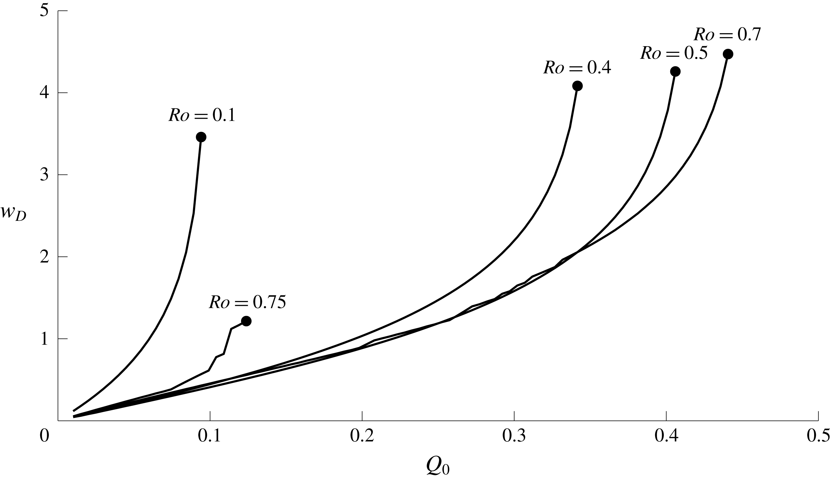
The width of the steady current
 $w_{D}$
downstream of the source, as a function of the total mass flux
 $Q_{0}$
, for various values of the Rossby number
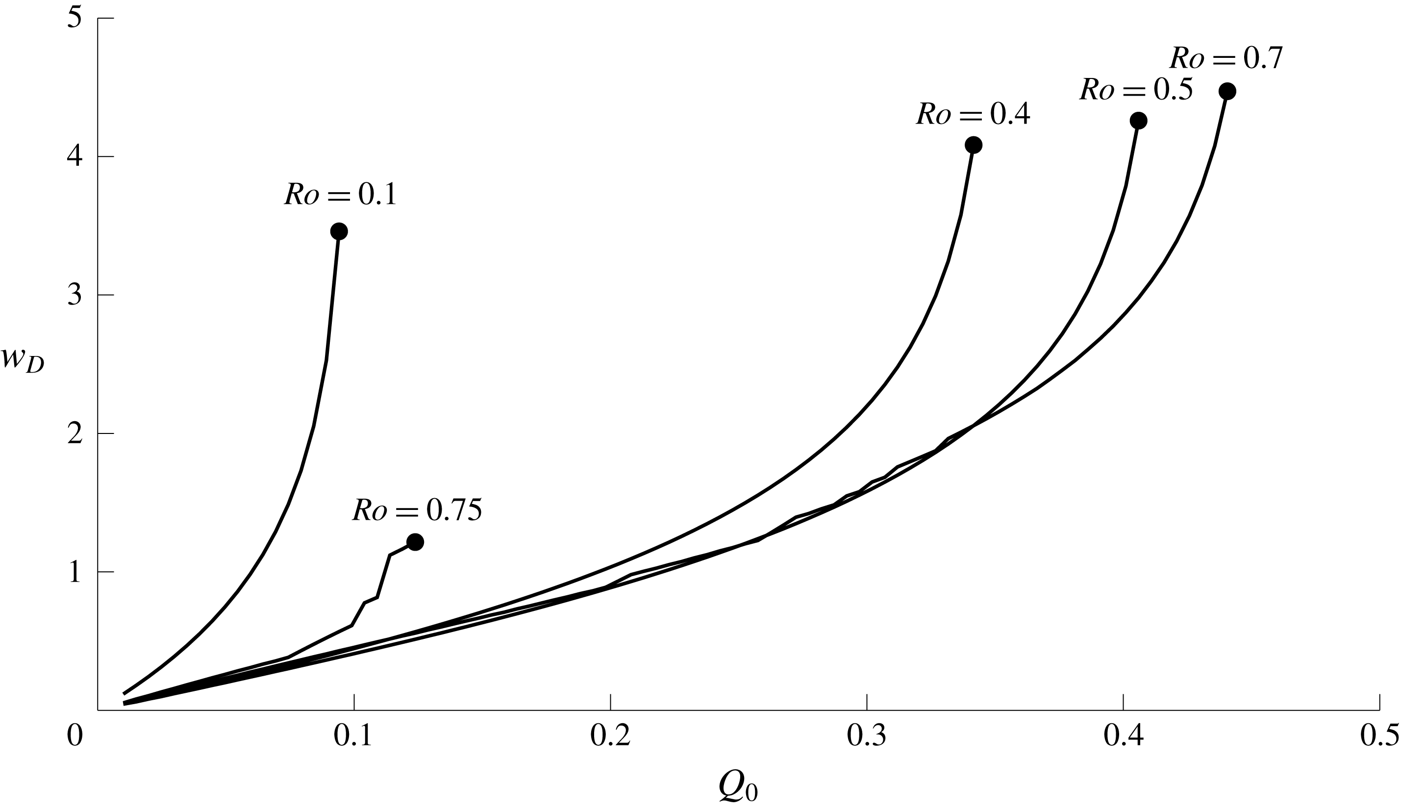
 $Ro$
.
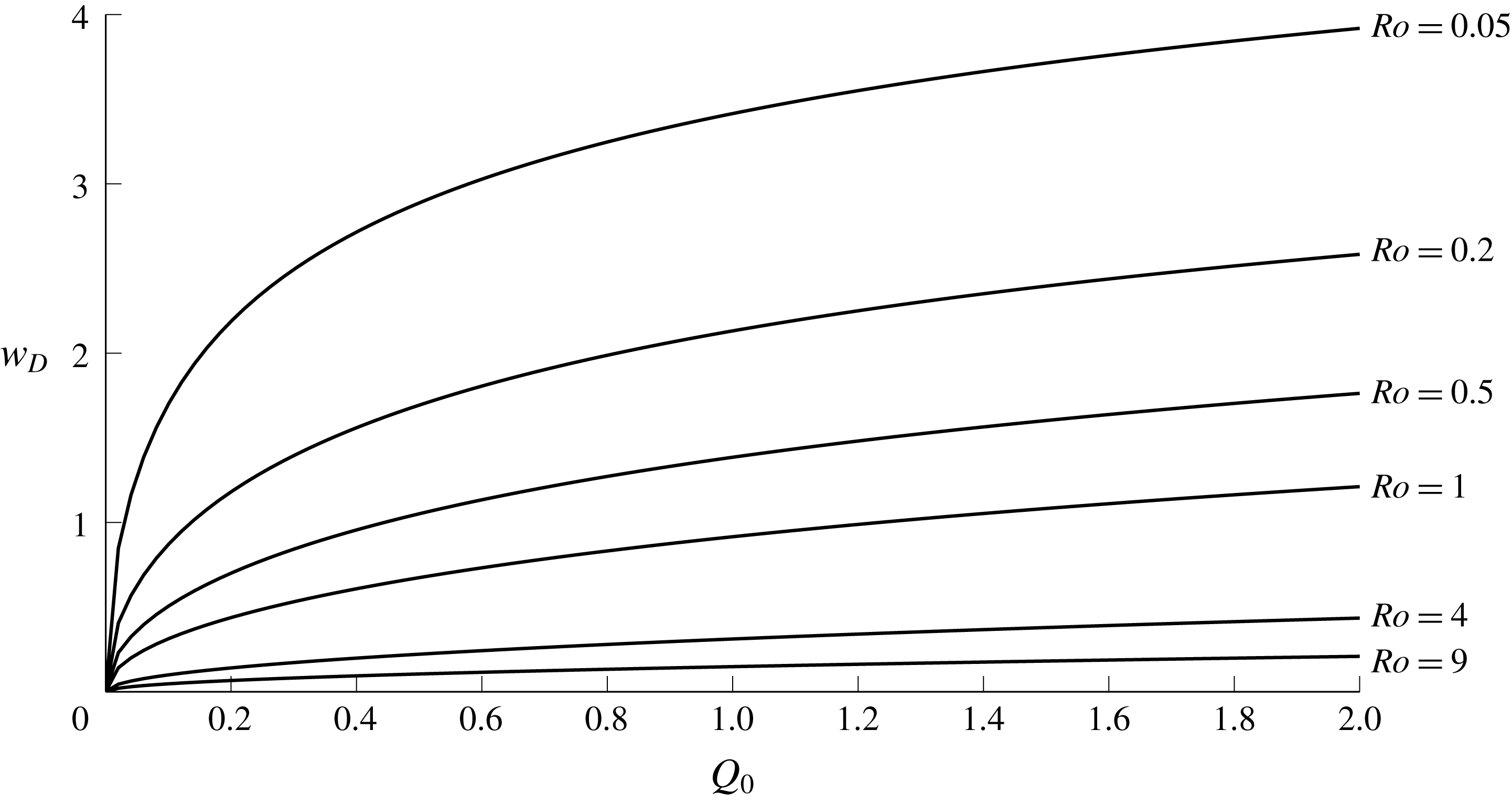
The downstream width of the steady solution
 $w_{D}$
is shown as a function of
 $Q_{0}$
and
 $H$
in figure 5. Since the steady solution always has
 $U=0$
, the river water completely adjusts to the upper-layer depth over the vortex scale
 $L_{V}$
in the source region. Large
 $Q_{0}$
– which corresponds to small
 $a$
and large
 $L_{V}$
– thus gives rise to a wider current (growing logarithmically as
 $Q_{0}\rightarrow \infty$
), while large
 $Ro$
gives small
 $L_{V}$
and a narrow current as the vortical turning happens closer to the wall. Because
 $w$
is scaled by the Rossby radius
 $L_{R}$
, the non-dimensional width of the steady current is equal to the Kelvin number
 $K$
, following Garvine (Reference Garvine1995). Figure 5 shows that
 $K>1$
in most flows and so the outflow behaviour is of the ‘large-scale’ type, i.e. significantly affected by rotation and geostrophically balanced.
The downstream constants of momentum and energy
 $S_{0}$
and
 $R$
can also be computed for steady solutions. From (2.20) and (2.10),
 $$\begin{eqnarray}S_{0}=\int _{0}^{Q_{0}}(H-1)\sqrt{\unicode[STIX]{x1D703}^{2}-1}\,\text{d}Q,\end{eqnarray}$$
where
 $\unicode[STIX]{x1D703}=\cosh (w_{sp})$
so that, from (3.6),
 $$\begin{eqnarray}(H-1)\sqrt{\unicode[STIX]{x1D703}^{2}-1}=\surd 2\sqrt{(H+Q-\surd (H^{2}+2Q))}=u_{W}.\end{eqnarray}$$
Analysis of the integral in (3.8) shows that
 $S_{0}$
grows like
 $Q_{0}^{3/2}$
as
 $Q_{0}\rightarrow \infty$
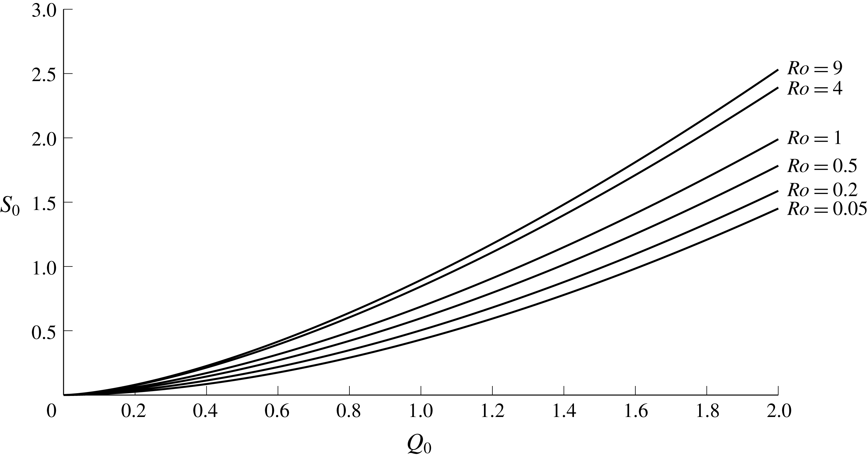
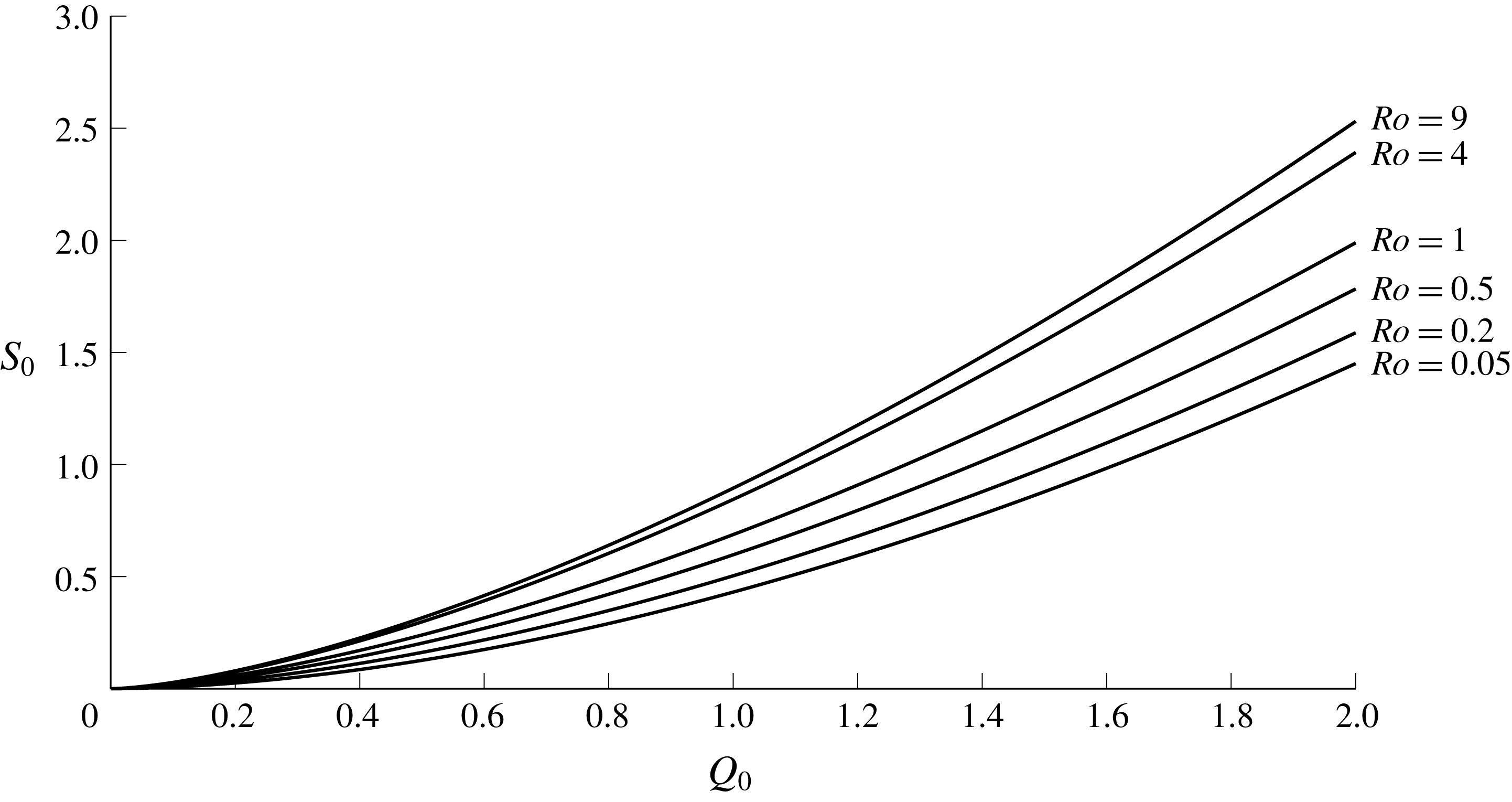
. Curves of
 $S_{0}$
for various parameter values are plotted in figure 6.
The total energy budget
 $R$
in the steady current is, from (2.21) and (3.9),
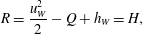 $$\begin{eqnarray}R=\frac{u_{W}^{2}}{2}-Q+h_{W}=H,\end{eqnarray}$$
as expected to match with the outer layer at
 $x=-1$
.
Momentum added by the source,
 $S_{0}$
, as a function of
 $Q_{0}$
and
 $Ro$
for positive PVa.
3.3 Downstream solution
Away from the source region the governing equations are unforced, and hence possess two Riemann invariants, i.e. there exist functions
 ${\mathcal{R}}_{C/R}(w,U)$
such that
 $$\begin{eqnarray}\frac{\text{d}}{\text{d}t}{\mathcal{R}}_{C/R}(w,U)=0\quad \text{on }\frac{\text{d}x}{\text{d}t}=\unicode[STIX]{x1D706}_{C/R}.\end{eqnarray}$$
Thus
 ${\mathcal{R}}_{C/R}$
are constant on each characteristic, with that constant determined by the values of
 $w$
and
 $U$
at the time when a given characteristic leaves the source region. For this system, the Riemann invariants cannot be found analytically and are obtained instead by solving the equivalent problem
 $$\begin{eqnarray}\frac{\text{d}U}{\text{d}w}=\unicode[STIX]{x1D6FC}_{C/R}(w,U)\quad \text{on }\frac{\text{d}x}{\text{d}t}=\unicode[STIX]{x1D706}_{C/R}\end{eqnarray}$$
as in Helfrich (Reference Helfrich2006). The functions
 $\unicode[STIX]{x1D6FC}_{C/R}$
are found by diagonalising the system (2.12)–(2.13), and are given explicitly in appendix A. The initial conditions for integrating (3.12) along a particular characteristic are given by the values of
 $w$
and
 $U$
at the point when that characteristic leaves the source region. In particular, once the steady solution reaches the downstream edge of the source region, the values of
 $w$
and
 $U$
are fixed and so all integrations start with the same conditions – the Riemann invariants are uniform.
The uniformity of one Riemann invariant is used in Stern & Helfrich (Reference Stern and Helfrich2002) to build similarity solutions
 $U(w)$
and describe the propagation of a coastal current with negative PVa. The same approach is applied here, whilst noting that uniform Riemann invariants only occur once the steady solution has been completely set up, and so the similarity solution is only valid after a finite time.
Immediately downstream of
 $x=1$
both Riemann invariants are uniform. Here, there are two universal relationships
 ${\mathcal{R}}_{C/R}(w,U)=m_{C/R}$
and so the only continuous solution has
 $w=w_{D}$
and
 $U=0$
(visible at late times in figures 3 and 4). The region of two uniform invariants is led by the slower characteristic
 $\unicode[STIX]{x1D706}_{R}$
, and so the speed at which the constant-width current spreads can be calculated by setting
 $w=w_{D}$
and
 $U=0$
in
 $\unicode[STIX]{x1D706}_{R}$
. Downstream of this constant-width region, only the
 $\unicode[STIX]{x1D706}_{C}$
characteristic is determined by the steady values of
 $w$
and
 $U$
and so only the
 ${\mathcal{R}}_{C}$
invariant is uniform. The similarity solution
 $U(w)$
can thus be found by integrating (3.12) away from the initial conditions
 $U=0$
,
 $w=w_{D}$
until the point
 $w=0$
, where we define
 $U(w=0)=U_{nose}$
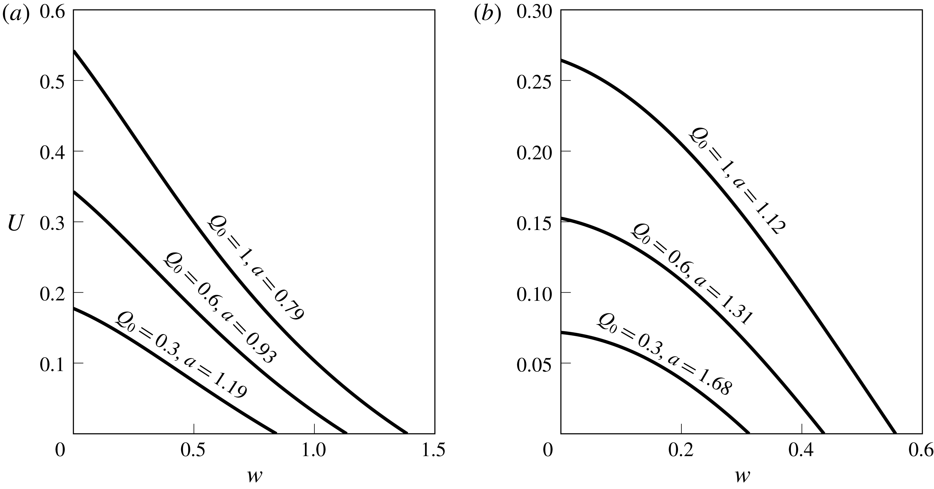
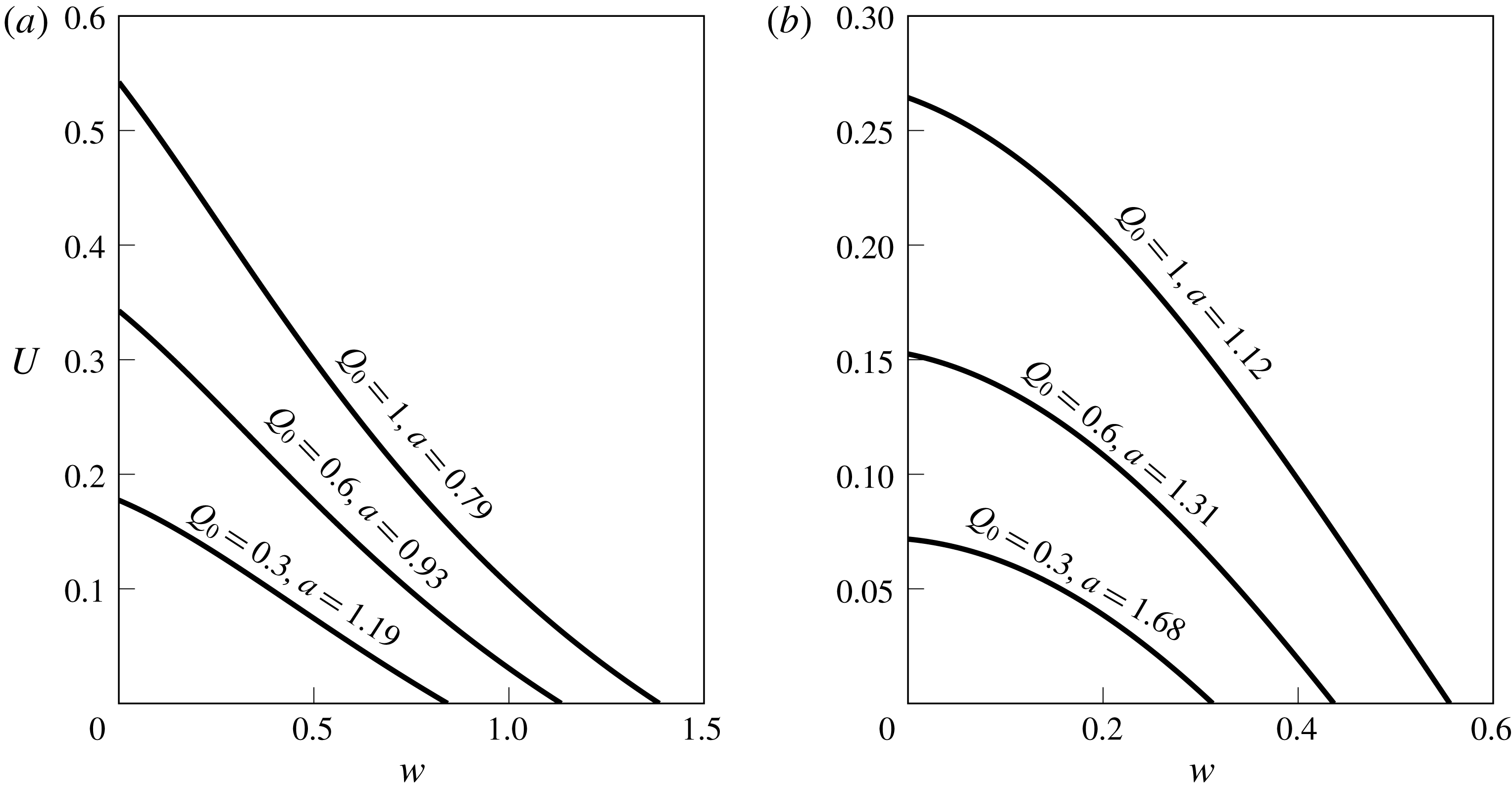
. Similarity solutions for various source fluxes are shown for
 $Ro=0.5$
and
 $Ro=2$
in figure 7. The solutions are all rarefactions (also called wedge intrusions or expansion waves) since they all have the property that
 $U$
increases as
 $w$
decreases. Rarefaction solutions have been previously described for coastal currents driven by PV jumps in Helfrich (Reference Helfrich2006) and JSM.
The velocity
 $U$
at the edge of the expelled fluid, as a function of the width
 $w$
, in the unsteady downstream rarefactions that lead the outflow. (a)
 $Ro=0.5$
, (b)
 $Ro=2$
. These relationships are valid once the steady solution has been set up across the source region.
3.3.1 Termination of the rarefaction
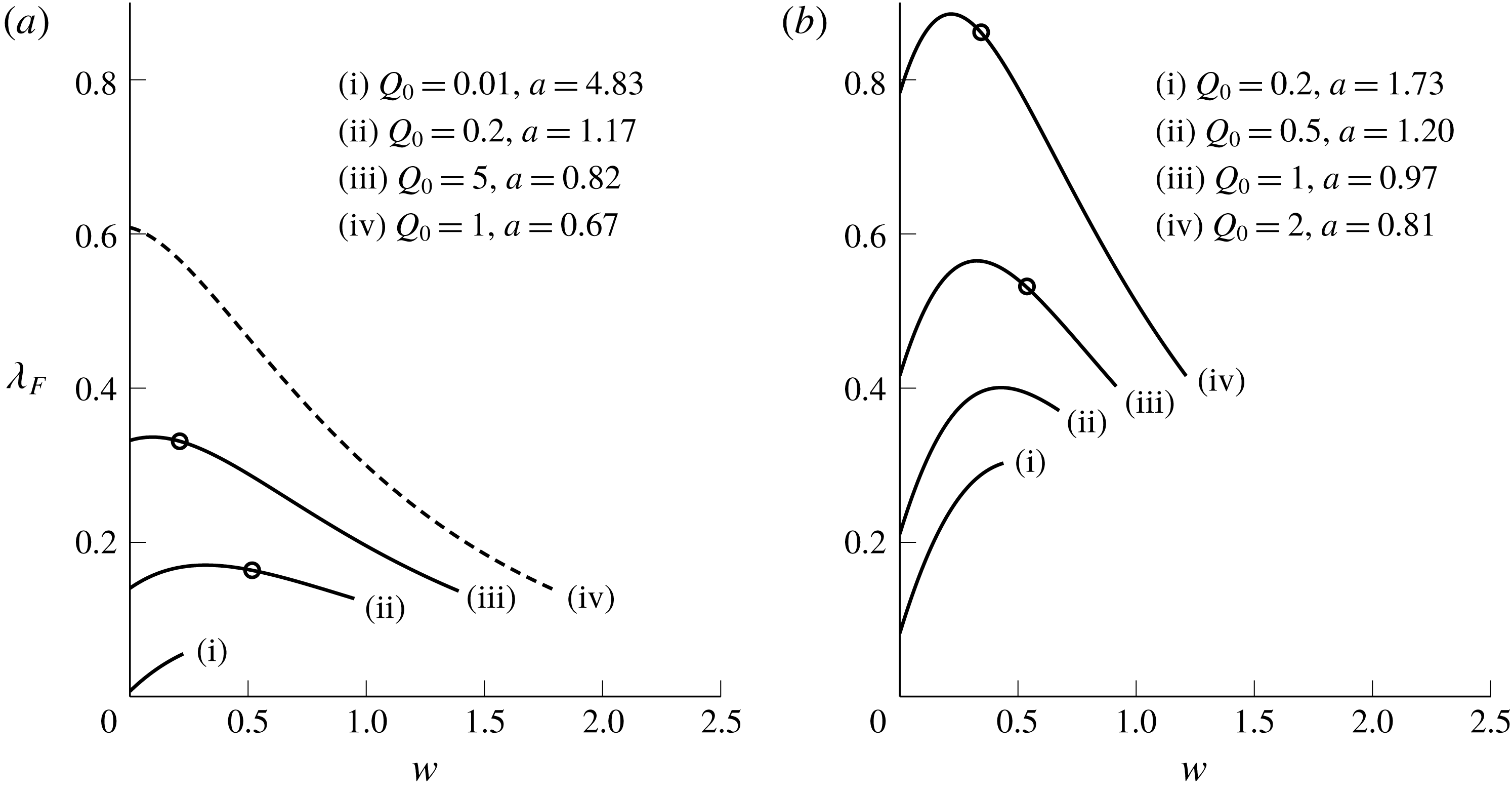
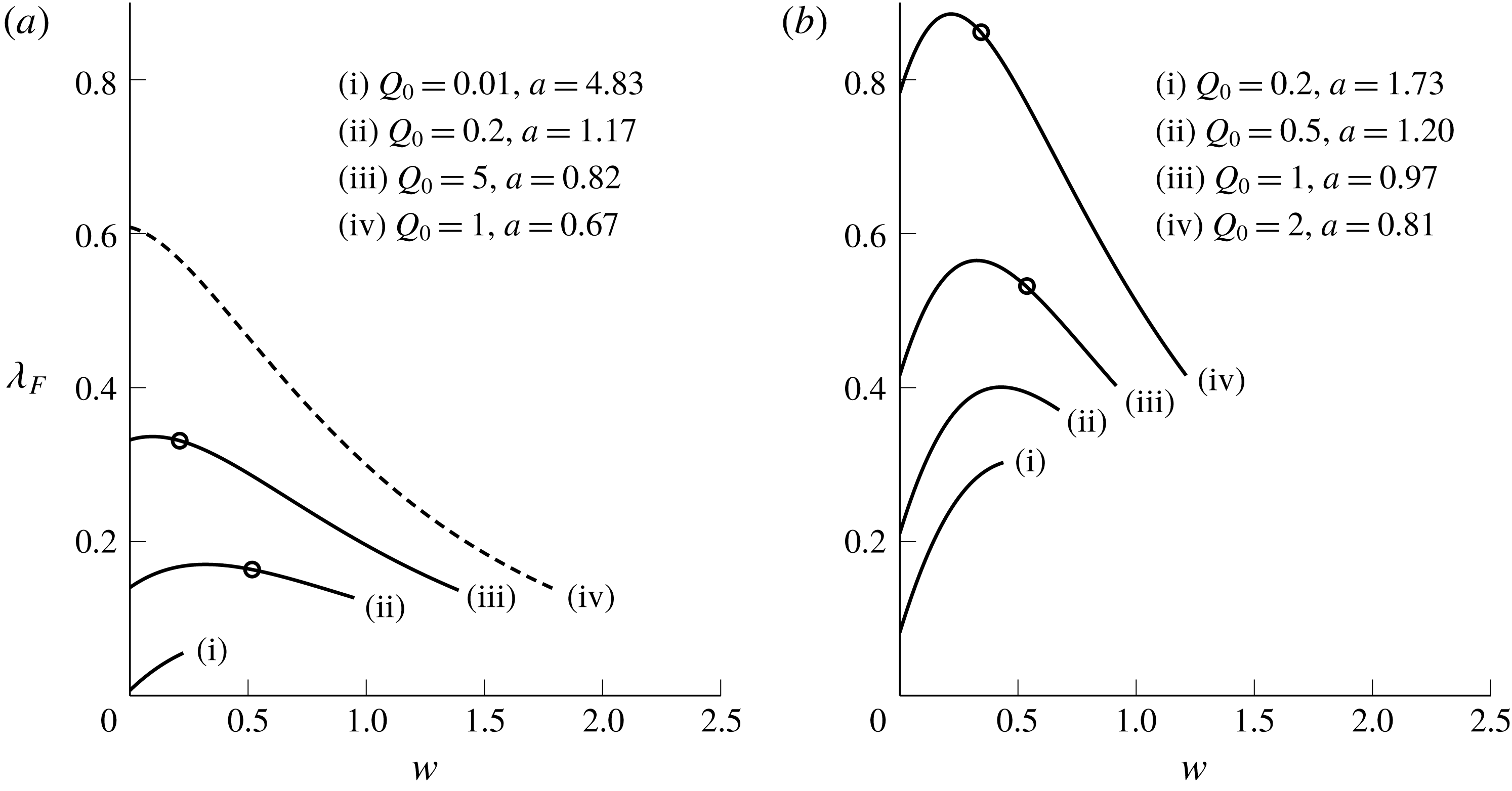
In regions where the similarity solution applies, the slope of the
 $\unicode[STIX]{x1D706}_{R}$
characteristics – those on which the Riemann invariant
 ${\mathcal{R}}_{R}$
is not uniform – can be computed as a function of
 $w$
only. This is done for various parameter values in figure 8.
Characteristic slope
 $\text{d}x/\text{d}t=\unicode[STIX]{x1D706}_{R}$
as a function of
 $w$
in regions where the similarity solution
 $U(w)$
applies (downstream of the source). The characteristic slopes are computed over the range
 $0\leqslant w\leqslant w_{D}$
and (a)
 $Ro=0.3$
, (b)
 $Ro=1$
. The dashed curve (a)(iv) does not form a shock, and circular markers on other curves indicate the maximum value of
 $w$
immediately behind the shock for that outflow. Solid curves without a marker develop shocks that increase in width until
 $w=w_{D}$
(a ‘blunt current’).
Since the solution grows monotonically in the source region, characteristics with larger values of
 $w$
leave the source later. Shocks form after a finite time if
 $\unicode[STIX]{x1D706}_{R}$
is not a monotonic decreasing function of
 $w$
, since characteristics with larger
 $\text{d}x/\text{d}t$
catch those with smaller
 $\text{d}x/\text{d}t$
. Differentiating the characteristic speed with respect to
 $w$
and evaluating at the wall gives
 $$\begin{eqnarray}\left.\frac{\text{d}\unicode[STIX]{x1D706}_{R}}{\text{d}w}\right|_{w=0}=\left.\frac{\unicode[STIX]{x2202}\unicode[STIX]{x1D706}_{R}}{\unicode[STIX]{x2202}w}+\frac{\unicode[STIX]{x2202}\unicode[STIX]{x1D706}_{R}}{\unicode[STIX]{x2202}U}\frac{\text{d}U}{\text{d}w}\right|_{w=0}=H-1+\frac{H-2}{\sqrt{H}}U_{nose}.\end{eqnarray}$$
A shock develops if (3.13) is positive. This occurs either if
 $H\geqslant 2$
, or if
 $$\begin{eqnarray}U_{nose}<\frac{\sqrt{H}(H-1)}{2-H}\end{eqnarray}$$
and
 $1<H<2$
. For large Rossby number (
 $H>2$
) a shock always forms, while for moderate or small Rossby number a shock forms only if the vortical current overturns at the wall and the nose velocity is sufficiently small. From the plots of
 $U_{nose}$
shown in figure 10, a slow nose velocity corresponds to smaller
 $Q_{0}$
(and bigger
 $a$
) and so, as in the quasi-geostrophic limit, vortically dominated flows are more likely to develop a shock. The dashed curve in figure 8(a)(iv) is the only one presented that does not develop a shock – note that it has the smallest
 $a$
of all solutions shown. The values of
 $Q_{0}$
beneath which a shock forms are marked on curves with
 $1<H<2$
in figure 10 below.
If no shock forms then the rarefaction is propagated by the
 $\unicode[STIX]{x1D706}_{R}$
characteristic, which reduce to
 $\unicode[STIX]{x1D706}_{R}=U$
when
 $w=0$
. The expelled fluid thus travels along the wall with velocity
 $U_{nose}$
and the fluid velocity is equal to the propagation velocity. If, on the other hand, a shock does form, then applying conservation of mass moving at the shock speed
 $V$
gives
 $$\begin{eqnarray}\int _{0}^{w}(u-V)h\,\text{d}y=0\end{eqnarray}$$
or
 $$\begin{eqnarray}V=\frac{(1+(-1+H+\sqrt{H}U)\cosh w+U\sinh w)^{2}-(H+\sqrt{H}U)^{2}}{2(w-U+U\cosh w+(-1+H+\sqrt{H}U)\sinh w)},\end{eqnarray}$$
where
 $U$
and
 $w$
are evaluated just behind the shock.
Because shocks form after a finite time, jumps in
 $w$
and
 $U$
are initially small and increase in magnitude until one of two things happens. If the shock velocity
 $V$
becomes equal to the characteristic speed
 $\unicode[STIX]{x1D706}_{R}$
, then at this point the shock and characteristic are tangential in the
 $(x,t)$
plane and no more information can enter the shock. That is, there exists some value
 $w_{M}$
such that
 $\unicode[STIX]{x1D706}_{R}(w_{M},U(w_{M}))=V(w_{M},U(w_{M}))$
. The solution is thus a rarefaction terminating in a shock, where the width of the shock approaches
 $w_{M}$
as
 $t\rightarrow \infty$
. The circular markers on characteristic curves in figure 8 indicate the value of
 $w_{M}$
for that particular
 $Q_{0}$
and
 $H$
. An example of such a solution is displayed in figure 4(a), where the value of
 $w_{M}$
is marked as a horizontal dashed line. Alternatively, the characteristic speed
 $\unicode[STIX]{x1D706}_{R}$
can be greater than
 $V$
for all
 $0<w<w_{D}$
. In this case, the shock keeps expanding until the maximum width of the current is reached, as seen in figure 3(b) where at late times the solution is simply a blunt current of width
 $w_{D}$
. This situation occurs when vortical effects are dominant and
 $a$
is large, as in the unmarked solid curves of figure 8. Note that a full-width shock will only develop if
 $\unicode[STIX]{x1D706}_{R}(w_{D})$
is greater than
 $V(w_{D},0)$
, so the qualitative behaviour of the solution as
 $t\rightarrow \infty$
can be determined by comparing these two values.
3.4 Interpretation in terms of the speed ratio
 $a$

From § 3.3, the qualitative behaviour of outflows can be categorised according to the form of the downstream current as a rarefaction joining smoothly to the wall, a rarefaction terminating in a shock, or a blunt current. The space of parameters
 $(Q_{0},H)$
can be divided into three regions, the boundaries of which can be computed efficiently by integrating the characteristic equation (3.12) and then applying the two tests described above to determine whether a shock forms and, if it does, whether the maximum jump magnitude is less than
 $w_{D}$
.
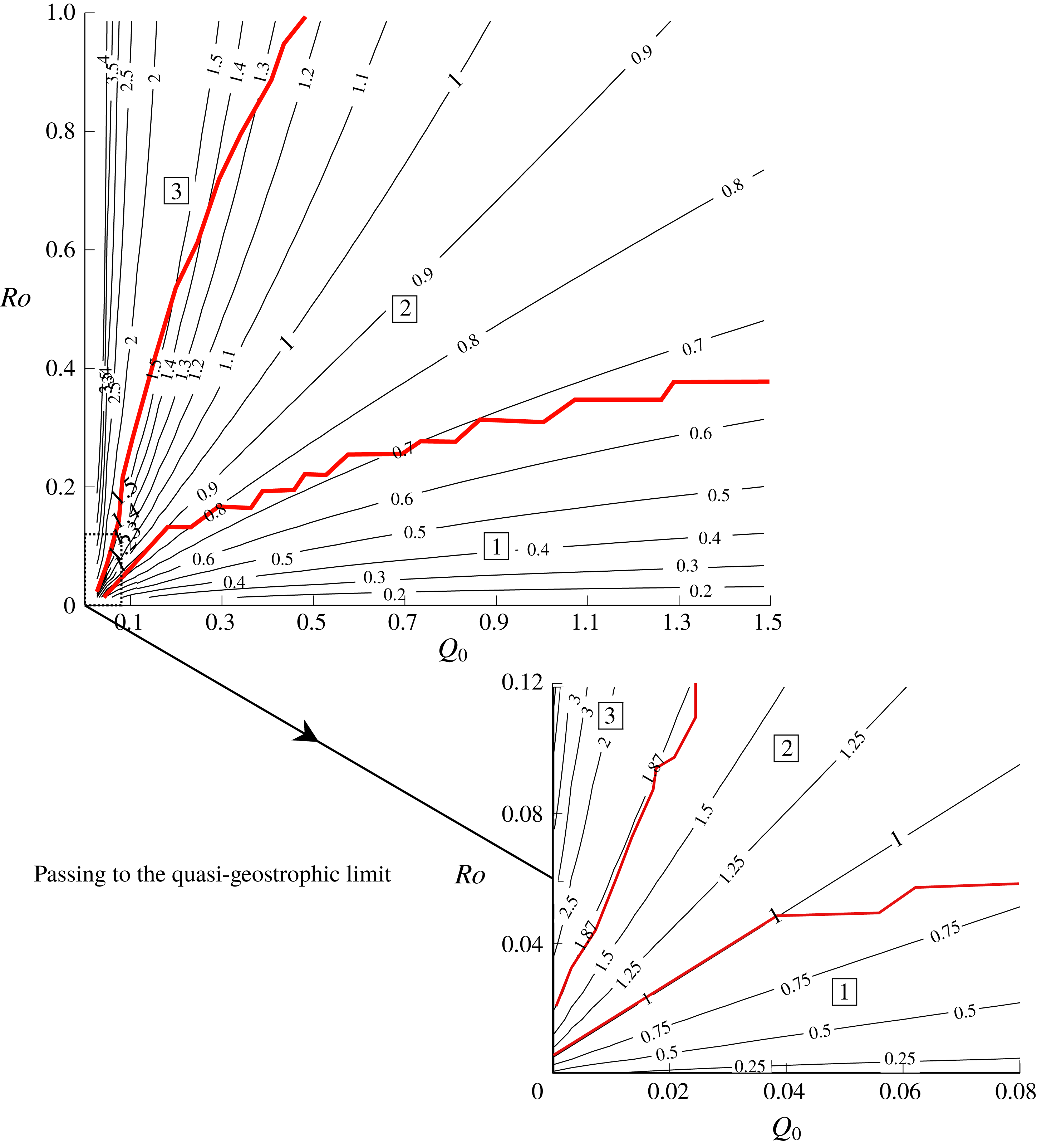
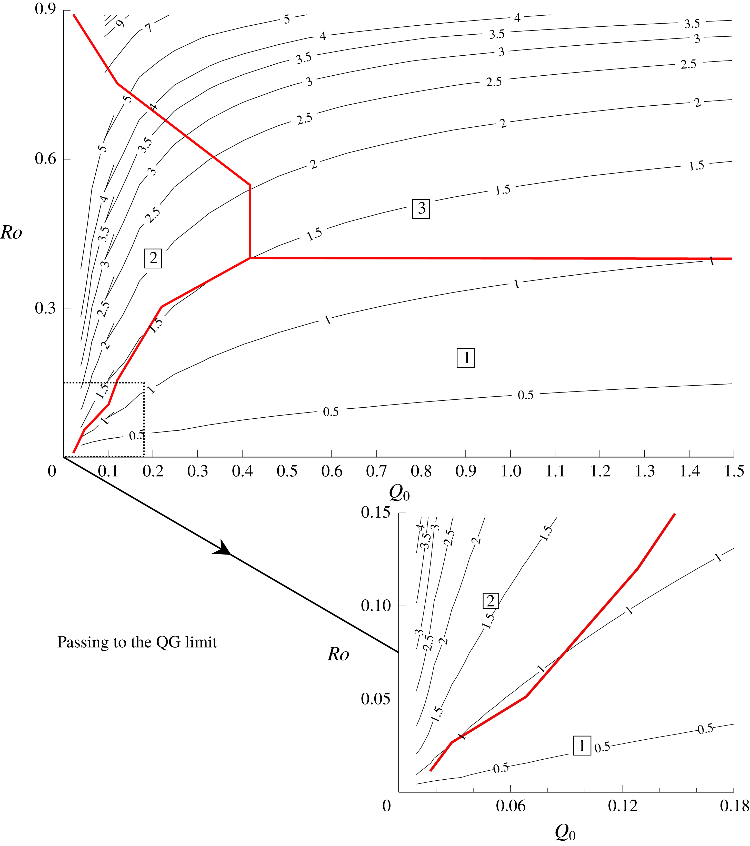
For positive PVa, the
 $(Q_{0},Ro)$
parameter space is divided into three regions (marked by thick lines, red online). Solution type one joins smoothly to the wall, solution type two is a rarefaction terminating in a shock, and solution type three is a full-width shock. Also shown are contours of the speed ratio
 $a$
. The inset details the behaviour in the quasi-geostrophic limit.
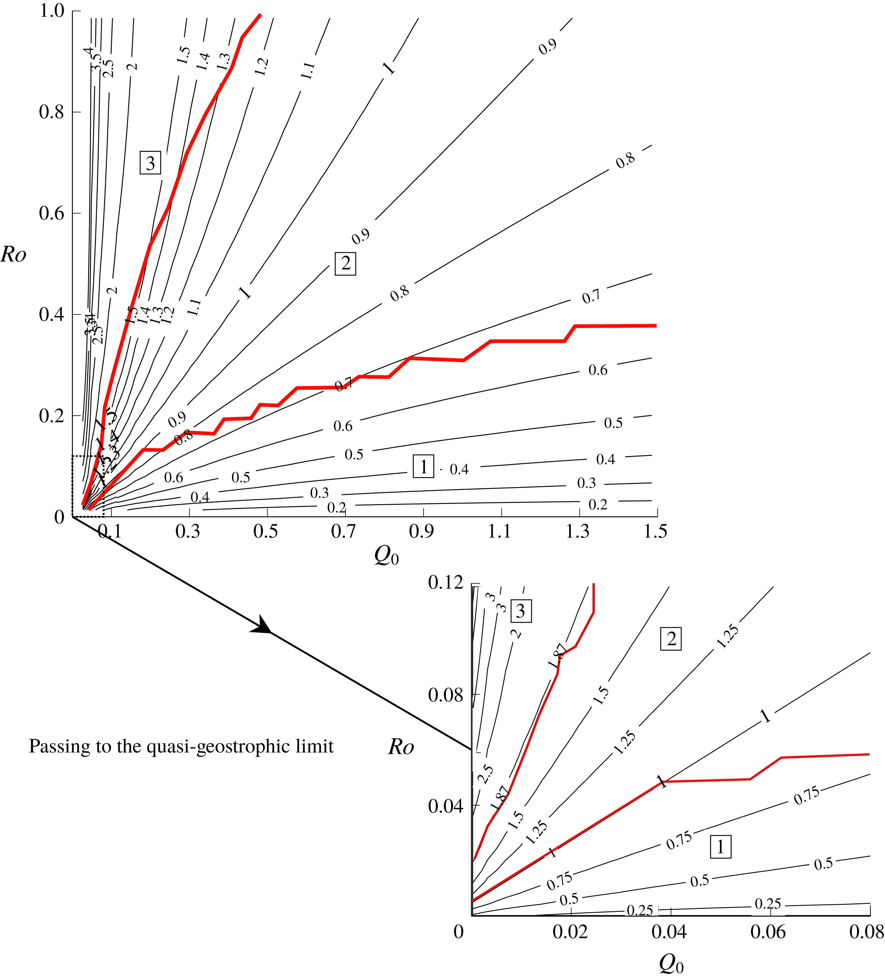
Figure 9 compares the numerically determined boundaries of these regions (numbered ‘1’, ‘2’ and ‘3’ respectively) with contours of
 $a$
, to illustrate the extent to which the flow behaviour depends on
 $Q_{0}$
and
 $H$
independently or whether, as in the quasi-geostrophic limit, the value of
 $a$
alone is sufficient to categorise the solution. In the quasi-geostrophic limit (inset) the region boundaries coincide precisely with the contours
 $a=1$
and
 $a=a_{m}\approx 1.87$
given in JSM. For larger
 $Ro$
and
 $Q_{0}$
, however, the region boundaries deviate from these values of
 $a$
, although the progression from no shock to partial-width shock and full-width shock with increasing
 $a$
remains.
3.5 Disturbance in the oceanic fluid
On the long-wave scale, the solution depends on
 $x$
through
 $U$
and
 $w$
alone. Information from the expelled fluid travels directly offshore into the oceanic fluid. This is at odds with, for example, the shallow-water numerical results of Helfrich (Reference Helfrich2006) (their figure 10) which shows waves that break ‘backwards’, and is a limitation of the long-wave assumption made here. From (2.7), this also means that regions where
 $U=0$
do not disturb the oceanic fluid, as shown in figure 4(c).
The similarity solutions obtained by integrating (3.12) give
 $U_{nose}$
: the value of
 $U$
at the point where
 $w=0$
, i.e. the fluid velocity at the leading edge of the expelled fluid. The horizontal dashed line in figure 4(b) marks the predicted value of
 $U_{nose}$
, and the figure also indicates that
 $U=U_{nose}$
in front of the expelled fluid, and thus that
 $U_{nose}$
is the coastal velocity of the Kelvin wave that travels ahead of the river water. This follows by noting that the similarity solution is valid anywhere that the
 ${\mathcal{R}}_{C}$
Riemann invariant is uniform; that is, at any point in the
 $(x,t)$
-plane occupied by a
 $\unicode[STIX]{x1D706}_{C}$
characteristic that left the source region after the steady solution was set up. In particular, this region extends beyond the nose of the river water and into the oceanic fluid. As discussed below, this then creates a shock in the oceanic fluid (the Kelvin-wave shock) and so all remnants of the initial conditions are erased with, at late times,
 ${\mathcal{R}}_{C}$
uniform everywhere that the fluid is disturbed. Note also that in vorticity-dominated flows where a shock develops in the river water, this is through the collision of
 $\unicode[STIX]{x1D706}_{R}$
characteristics and so
 ${\mathcal{R}}_{C}$
is conserved across the shock (El Reference El2005). The similarity solution thus remains valid at the nose of river water, and
 $U=U_{nose}$
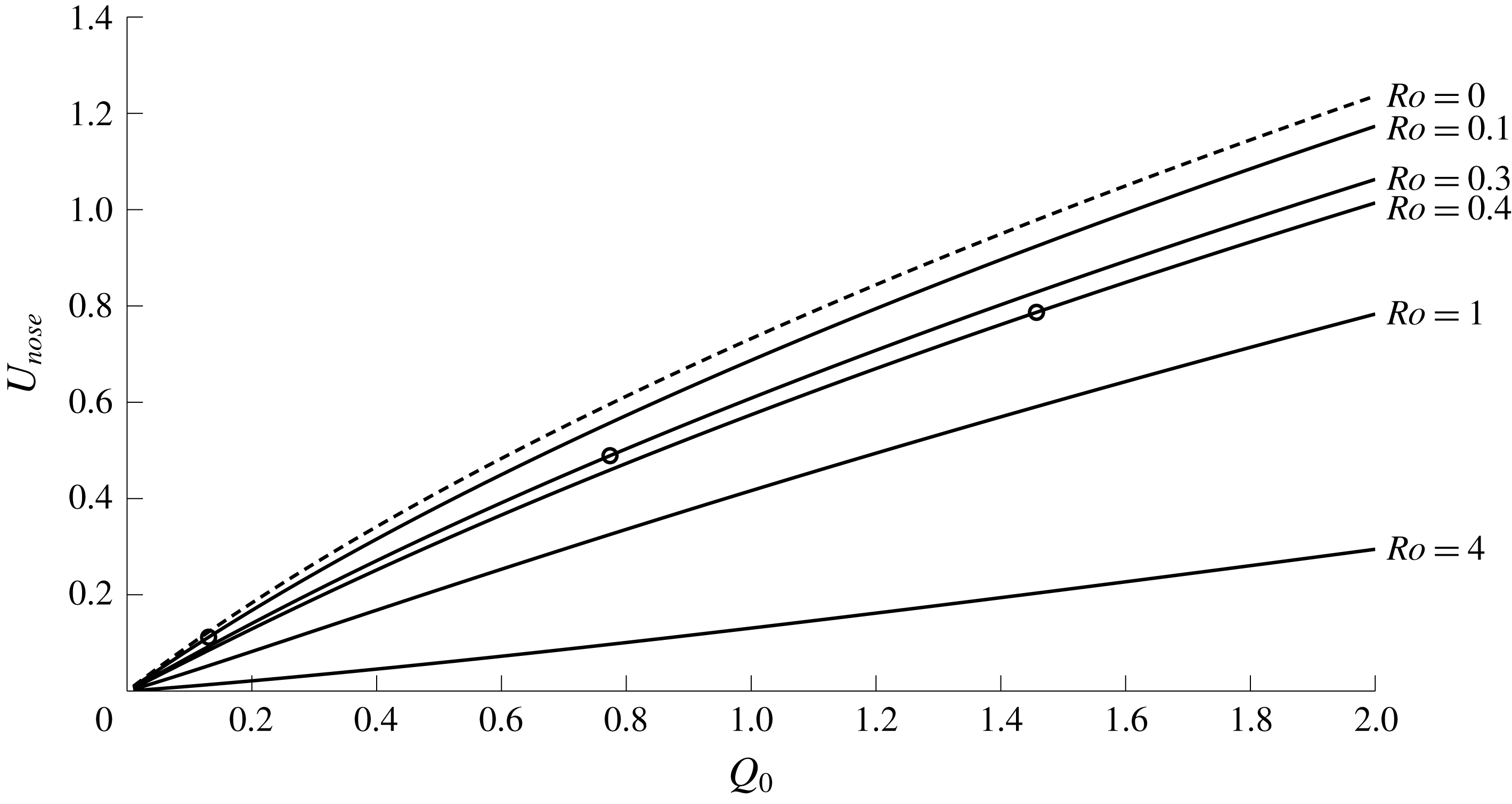
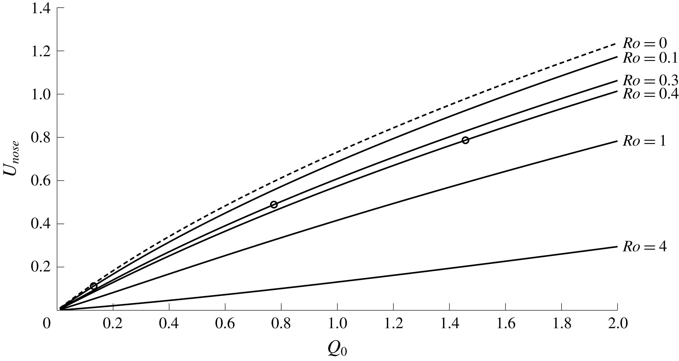
ahead of the expelled fluid. Curves showing
 $U_{nose}$
as a function of the total mass flux are presented in figure 10 for various
 $Ro$
, along with the speed of the Kelvin-wave-driven flow
 $u_{KW}$
(dashed).
Nose speed for various
 $Ro$
as a function of the source mass flux
 $Q_{0}$
. The ‘nose speed’ refers to the along-wall velocity of fluid in the Kelvin wave that propagates ahead of the river water. Circles mark the value of
 $Q_{0}$
below which a shock forms in the expelled fluid, and curves without circles always form a shock. Also shown (dashed) is the wall velocity of the zero PVa solution.
The motion in the oceanic fluid ahead of the river fluid is governed by (2.12) with
 $w=0$
,
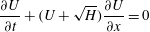 $$\begin{eqnarray}\frac{\unicode[STIX]{x2202}U}{\unicode[STIX]{x2202}t}+(U+\sqrt{H})\frac{\unicode[STIX]{x2202}U}{\unicode[STIX]{x2202}x}=0\end{eqnarray}$$
(cf. the zero-PVa equation (2.23)). The propagation speed ahead of the river water is therefore the sum of
 $\sqrt{H}$
, the non-dimensional speed of the linear Kelvin wave, and a nonlinear advection at speed
 $U$
. For a fixed volume flux
 $Q_{0}$
, increasing the oceanic layer depth, and so increasing
 $Ro$
, corresponds to lower fluid velocity
 $U$
. This decrease in
 $U$
dominates the increase in
 $H$
, causing the nose speed
 $U_{nose}$
to decrease as seen in figure 10.
Solutions to (3.17) always develop a shock when
 $U$
is a decreasing function of
 $x$
, as seen in the development of figure 4(b). Once a shock forms, the jump height increases until
 $U=U_{nose}$
and the shock propagates into the resting fluid at a speed determined by the relevant Rankine–Hugoniot condition to be
 $$\begin{eqnarray}V_{KW}=\frac{U_{nose}}{2}+\sqrt{H}.\end{eqnarray}$$
The horizontal vertical lines in figure 4(b) are separated by
 $3V_{KW}$
, and match well with the solutions at
 $t=9,12$
even though
 $U$
has not quite reached
 $U_{nose}$
. A full three-dimensional model of such shocks is considered in Fedorov & Melville (Reference Fedorov and Melville1996), and the propagation speed here agrees with their relation (7.20).
4 Outflows with negative PVa
When the expelled fluid has negative PV anomaly (
 $H<1$
), the image vorticity opposes the Kelvin-wave-driven flow, and fluid travels both upstream and downstream. JSM show that steady flow only occurs if the outflow is vortically dominated (
 $a>1$
); otherwise the current expands indefinitely in the source region. These two behaviours correspond to the gyre mode and the widening coastal mode described in Kubokawa (Reference Kubokawa1991). For the positive PVa outflows of § 3, fluid travels downstream only and the oceanic layer is undisturbed in
 $x<-1$
. This matching condition leads to a full description of the steady current in the source region, which then provides initial conditions for integrating (3.12) and the theory that describes the rarefaction solution. For outflows with negative PVa, fluid is disturbed both upstream and downstream and so analogous matching conditions do not exist. For outflows that evolve to become steady across the source region, an asymptotic theory based on properties of the steady quasi-geostrophic solution can be derived, and this is shown to agree well with numerical results even at moderate
 $Ro$
.
4.1 Numerical results
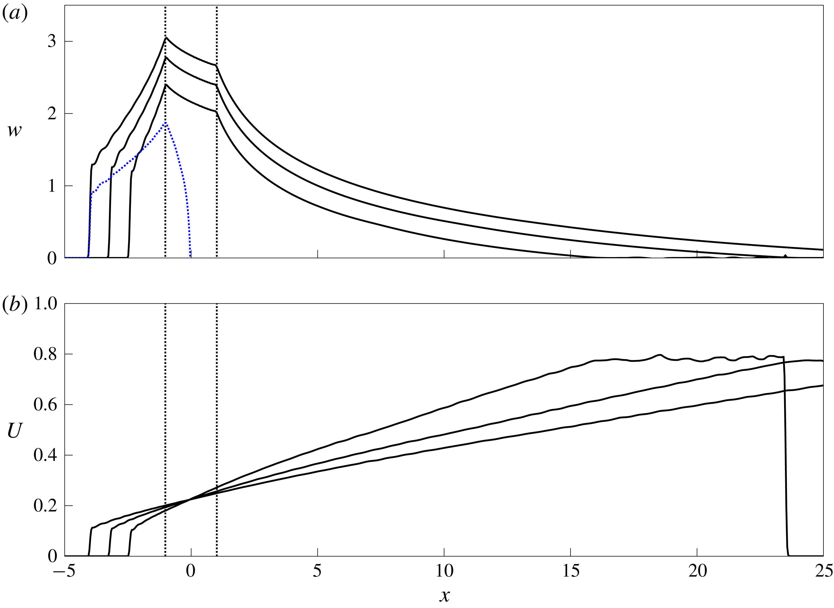
An outflow with negative PVa,
 $Ro=0.4$
,
 $Q_{0}=0.7$
and
 $a=1.24$
at times
 $t=20,30,40$
. (a) The current width
 $w$
, which continues increasing across the source region (marked by vertical dotted lines). The dotted curve (blue online) gives the curve
 $y=\tilde{w}$
along which
 $u=0$
(at
 $t=40$
). (b) The edge velocity
 $U$
at
 $t=20,30,40$
.
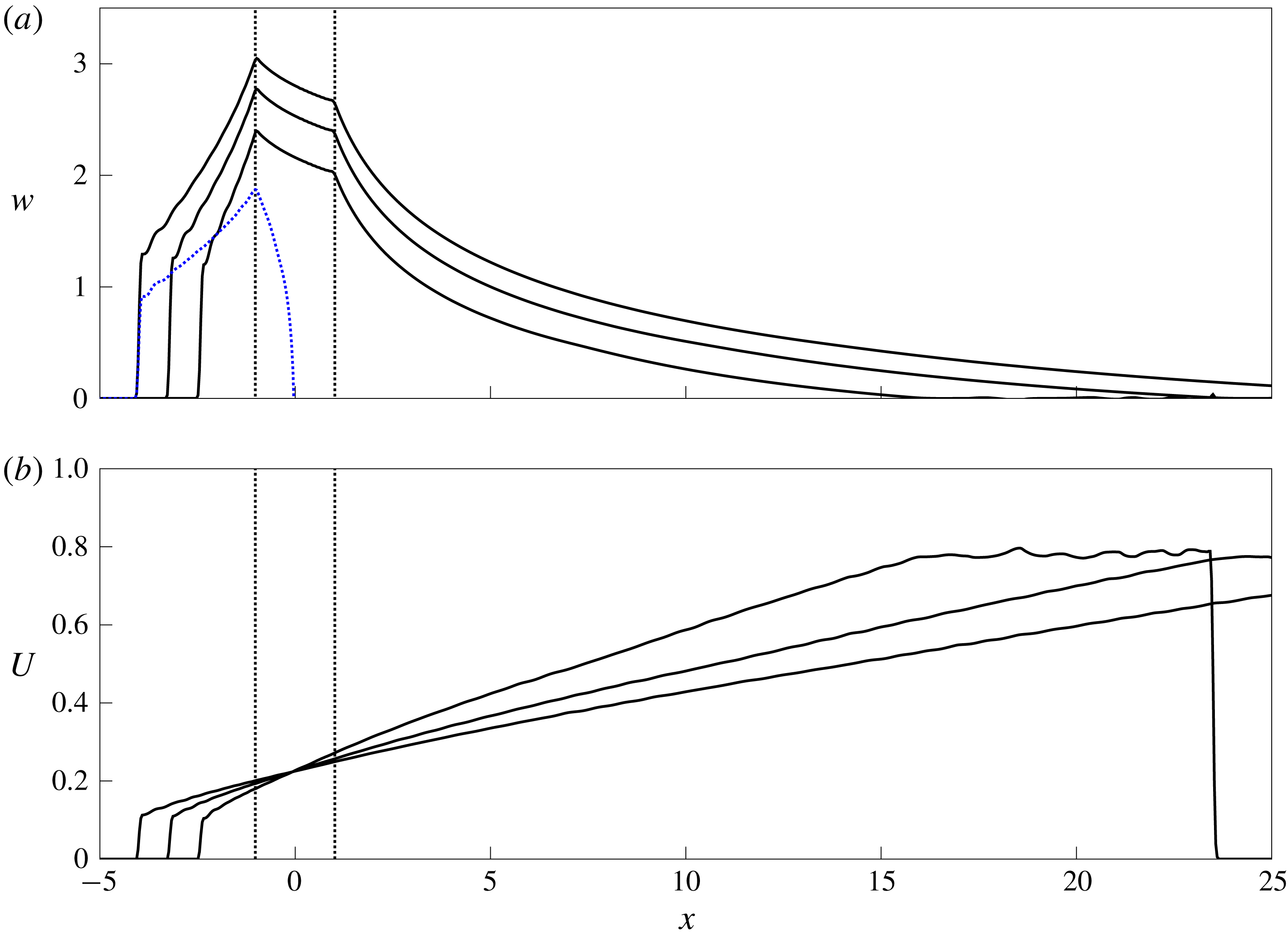
An example of an unsteady, widening current is shown in figure 11 where
 $Ro=0.4$
,
 $Q_{0}=0.7$
and so
 $a=1.24$
. Since
 $a>1$
the outflow is vortically dominated and the corresponding quasi-geostrophic flow would evolve to become steady across the source region. Here, however,
 $Ro$
is sufficiently large that the current width continues to grow. Some expelled fluid travels downstream, joining smoothly to the wall in a rarefaction with, as for positive PVa, a Kelvin wave travelling ahead in the outer layer. The rest of the expelled fluid travels upstream. The boundary between fluid moving upstream and fluid moving downstream, where
 $u=-h_{y}=0$
(and so the outflow depth is at a maximum), is denoted
 $y=\tilde{w}(x,t)$
and shown dotted (blue online) in figure 11(a). Fluid thus travels upstream along the wall, before turning and heading downstream around the edge of the current, taking oceanic water with it as
 $U>0$
. Thus one important difference between solutions with positive and negative PVa is that outflows with negative PVa transport oceanic fluid from upstream of the source region to downstream. Computation of the off-shore velocity
 $v$
reveals that fluid travels at infinite velocity around the upstream boundary of the outflow before heading downstream. This failure of the semi-geostrophic equations is due to the short length scales in the shock region, as noted by Helfrich (Reference Helfrich2006).
Solutions to the outflow problem with negative PVa,
 $Ro=0.5$
,
 $Q_{0}=0.2$
and
 $a=2.44$
at times
 $t=20,40,120$
. (a) The current width
 $w$
, which is steady across the source region (marked by vertical dotted lines). The (green) dashed line at
 $x\approx -6$
indicates the location of the transect used to compare with experimental solutions in § 5. (b) The velocity
 $U$
at the current edge. The thick dashed curves (red online) are the steady solutions
 $w_{sn}$
and
 $U_{c}$
from § 4.2, the blue dotted line is
 $y=\tilde{w}$
, and the black dashed lines are derived from the theory of § 4.3 and discussed there. (c) Contours of the depth perturbation
 $h-H$
at
 $t=40$
, where the shaded region indicates the expelled fluid.

Figure 12 shows an example of a steady current where
 $Ro=0.5,Q_{0}=0.2$
and
 $a=2.44$
. In steady solutions, the curve
 $y=\tilde{w}$
(dotted, blue online) touches the wall at
 $x=1$
, thus
 $u_{W}=0$
here and all the outflow first heads upstream before a portion recirculates to form the downstream current, which again is a rarefaction. In all solutions with negative PVa, condition (3.14) cannot be satisfied with
 $U>0$
and so the downstream rarefaction joins smoothly to the wall, demonstrating the importance of vortical flow in the formation of leading shocks. The steady solution is very similar to that of McCreary et al. (Reference McCreary, Zhang and Shetye1997) (their figure 9) where upstream flows are driven by geostrophic adjustment of a density front. The upstream solution here is similar to the downstream solution for positive PVa: a constant-width region near the source, then a rarefaction terminating in a leading shock. Figure 12(b) shows the edge velocity
 $U$
, and the ripples visible at late times are the result of numerical dispersion. Figure 12(c) shows contours of the layer-depth perturbation
 $h-H$
at
 $t=40$
. The river fluid is shaded, with the region where
 $u<0$
shaded darker. The Kelvin wave is again seen to travel ahead of the river water and disturb the oceanic fluid. The contour closest to the coast has a negative value: the outflow has caused a shallowing of the layer upstream of the source.
4.2 Steady solutions across the source region
Since the oceanic layer is disturbed both upstream and downstream of the source, there are no matching conditions to determine the constants of integration and obtain a steady solution as in § 3.2. Instead, specifying the constants requires two additional relations, which are based on quasi-geostrophic theory and later verified against numerical results to the initial-value problem.
First, note that one family of characteristic slopes
 $\unicode[STIX]{x1D706}_{C}$
are always positive (see appendix A), while the other set
 $\unicode[STIX]{x1D706}_{R}$
vanishes whenever
 $u_{W}=0$
, i.e.
 $U=U_{c}$
, say, where
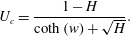 $$\begin{eqnarray}U_{c}=\frac{1-H}{\coth (w)+\sqrt{H}}.\end{eqnarray}$$
Now
 $U_{c}<0$
when
 $H>1$
but
 $U_{c}>0$
when
 $H<1$
, allowing
 $\unicode[STIX]{x1D706}_{R}$
to send information upstream if the PVa is negative, and thus the
 $\unicode[STIX]{x1D706}_{R}$
characteristic is associated with the vortical flow, and
 $\unicode[STIX]{x1D706}_{C}$
with the Kelvin-wave-driven flow, as noted for the special case
 $H=0$
in Kubokawa & Hanawa (Reference Kubokawa and Hanawa1984a
).
As in outflows with positive PVa, steady currents are controlled at the edge of the source region. In particular there exists a separatrix, i.e. a characteristic
 $\unicode[STIX]{x1D706}_{R}$
that has a turning point at
 $x=1$
. Characteristics that start to the right of the separatrix end up downstream of the source, and those that start to the left go upstream. There is thus a region in the wake of the turning point of the separatrix where characteristics that originate at
 $t=0$
cannot penetrate, and characteristics instead propagate out from the turning point, where (4.1) is satisfied. The steady solution thus spreads upstream across the source region, starting at the downstream edge where it is controlled by the
 $\unicode[STIX]{x1D706}_{R}$
characteristic. Physically, this sets
 $u_{W}=0$
at the downstream edge of the source region and shows that, for steady solutions, all of the outflow must first head upstream driven by image vorticity, as seen in figure 12(c). There are, however, an infinite number of steady solutions that satisfy this control condition, and a further equation is needed to close the system.
Note that the curve
 $y=\tilde{w}$
, on which
 $u=0$
, can be computed from (2.7) as
 $$\begin{eqnarray}\tilde{w}=w-\log \left(\frac{\sqrt{H-1-U+\surd HU}}{\sqrt{H-1+U+\surd HU}}\right)\end{eqnarray}$$
so that
 $w-\tilde{w}$
is constant for steady solutions. Using (4.2), the system can be closed with one further relationship between
 $w$
and
 $\tilde{w}$
. This is equation (21) in McCreary et al. (Reference McCreary, Zhang and Shetye1997),
 $$\begin{eqnarray}\tilde{w}_{\infty }={\textstyle \frac{1}{2}}\log (2\text{e}^{w_{\infty }}-1),\end{eqnarray}$$
where the subscript refers to values evaluated far upstream at late times, after a steady current has completely developed. In McCreary et al. (Reference McCreary, Zhang and Shetye1997), (4.3) is derived by taking the first term in an asymptotic expansion of a mass-balance equation similar to (3.15), which effectively requires that the coastal depth change is small relative to
 $H$
. As such, (4.3) is also the relationship between
 $w$
and
 $\tilde{w}$
in the quasi-geostrophic solutions of JSM and so must hold for small
 $Ro$
and
 $Q_{0}$
in the semi-geostrophic problem. We thus develop here a theory assuming that (4.3) holds for all values of
 $Q_{0}$
and
 $Ro$
, and then verify numerically that this asymptotic approximation captures the qualitative behaviour of the outflow even at moderate
 $Q_{0}$
and
 $Ro$
.
Given the conditions (4.1)–(4.3), the relevant solution to the steady equations (3.4) can be most succinctly described as
 $$\begin{eqnarray}w_{sn}(Q)=\log \left(\frac{r(Q)+\sqrt{r(Q)^{2}+k^{2}-1}}{1+k}\right),\end{eqnarray}$$
where
 $$\begin{eqnarray}k=\frac{U}{H-1+\sqrt{H}U},\quad r(Q)=\frac{\sqrt{2(Q+c)}-1}{H-1+\sqrt{H}U}\end{eqnarray}$$
and
 $c$
and
 $U$
are determined by applying (4.1)–(4.3). The heavy dashed curves (red online) in figure 12 give
 $w_{sn}$
and
 $U_{c}$
, both of which give good agreement with the numerical results even at
 $Ro=0.5$
.
Figure 13 shows the downstream width of the steady current
 $w_{sn}(Q_{0})=w_{D}$
. As for positive PVa, for a given
 $Ro$
the downstream current width increases with increasing mass flux. For fixed
 $Q_{0}$
, the width does not increase monotonically with
 $Ro$
. As the magnitude of the PVa is increased, the current first contracts (in line with the results for positive PVa) before expanding again after
 $Ro\approx 0.6$
. Numerical computations show that for a given
 $Ro$
there is a maximum flux
 $Q_{0}$
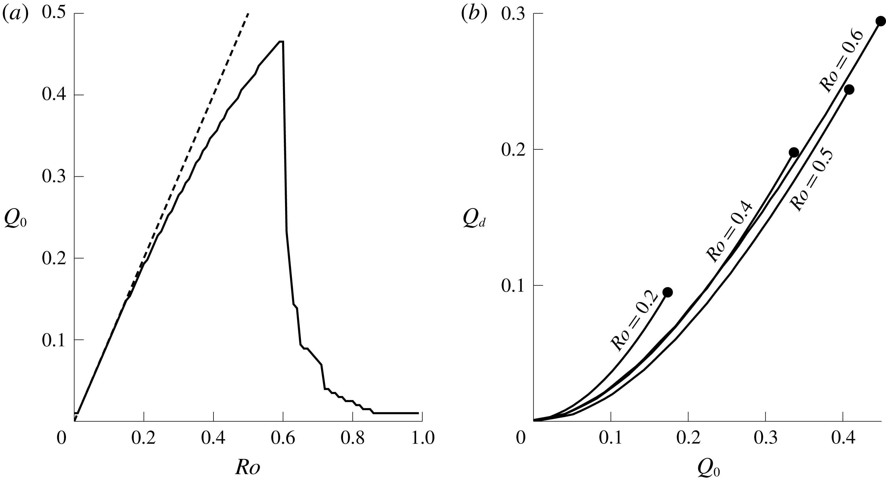
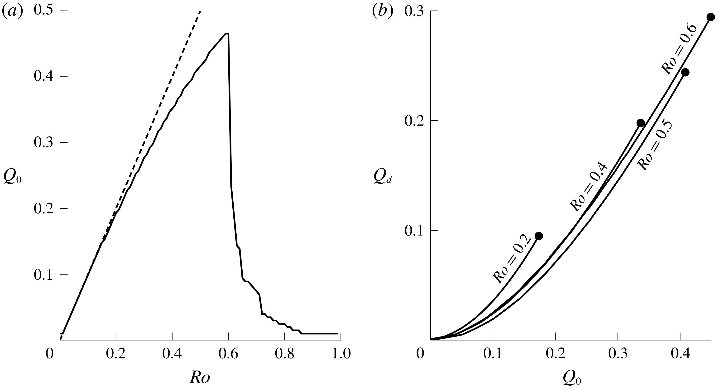
for which both (4.1) and (4.3) can be solved simultaneously, and thus an upper bound on the mass flux that supports a steady solution (marked by a dot in figure 13). The limited capacity of coastal currents to transport fluid with negative PVa was remarked on in Kubokawa (Reference Kubokawa1991) and observed in laboratory experiments in Horner-Devine et al. (Reference Horner-Devine, Fong, Monismith and Maxworthy2006). Figure 14(a) shows this maximum flux, which is not a monotonic function of
 $Ro$
– a result discussed in more detail in § 4.4. Also marked (dashed) in figure 14(a) is the line
 $Q_{0}=Ro$
, which is the maximum flux that supports a steady solution in the quasi-geostrophic limit.
The steady solution width at the downstream edge,
 $w_{D}$
, as a function of the flux
 $Q_{0}$
. The largest
 $Q_{0}$
for which a steady solution exists at a given
 $Ro$
is marked by a dot.
In addition to the upper bound on
 $Q_{0}$
at fixed
 $Ro$
, there is an absolute maximum of
 $Q_{0}$
over all
 $Ro$
that supports a steady current. For real solutions, (4.4) requires that
 $r$
is positive. Expression (4.1) shows that
 $U<1-\sqrt{H}$
and so the denominator of
 $r$
is negative, and so therefore the numerator must also be negative, giving
 $Q+c<1/2$
. As
 $Q$
and
 $c$
are non-negative, they must both individually be less than
 $1/2$
. Thus no controlled steady solution exists when
 $Q_{0}>1/2$
, as in the similar relation obtained in Whitehead & Salzig (Reference Whitehead and Salzig2001) for flow out of a wide basin.
For negative PVa, only a portion of the outflow recirculates and so the downstream flux
 $Q_{d}$
, given by
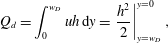 $$\begin{eqnarray}Q_{d}=\int _{0}^{w_{D}}uh\,\text{d}y=\left.\frac{h^{2}}{2}\right|_{y=w_{D}}^{y=0},\end{eqnarray}$$
is less than the total flux
 $Q_{0}$
. Profiles of
 $Q_{d}$
as a function of
 $Q_{0}$
are shown for various
 $Ro$
in figure 14(b). The curve for
 $Ro=0.6$
lies above that for
 $Ro=0.5$
, in accord with the non-monotonic behaviour of the total flux shown in (a).
Mass flux for steady solutions with negative PVa. (a) The maximum mass flux supported by a given
 $Ro$
. (b) The downstream mass flux
 $Q_{d}$
as a function of total mass flux
 $Q_{0}$
, for various
 $Ro$
.
The momentum and energy constants
 $S_{0}$
and
 $R$
can also be computed for steady solutions. Since
 $u_{W}<0$
throughout the source region, the momentum input (2.20) across the source is negative:
 $$\begin{eqnarray}S_{0}=-\sqrt{2}\int _{0}^{Q_{0}}\sqrt{(Q-Q_{0}+\sqrt{2(Q_{0}+c)}-\sqrt{2(Q+c)})}\,\text{d}Q.\end{eqnarray}$$
The energy constant
 $R$
can be determined by evaluating (2.21) at the point
 $x=1,y=0$
. Here
 $u=0$
and
 $\unicode[STIX]{x1D713}=Q_{0}$
, so
 $$\begin{eqnarray}R=\sqrt{2(Q_{0}+c)}-Q_{0}.\end{eqnarray}$$
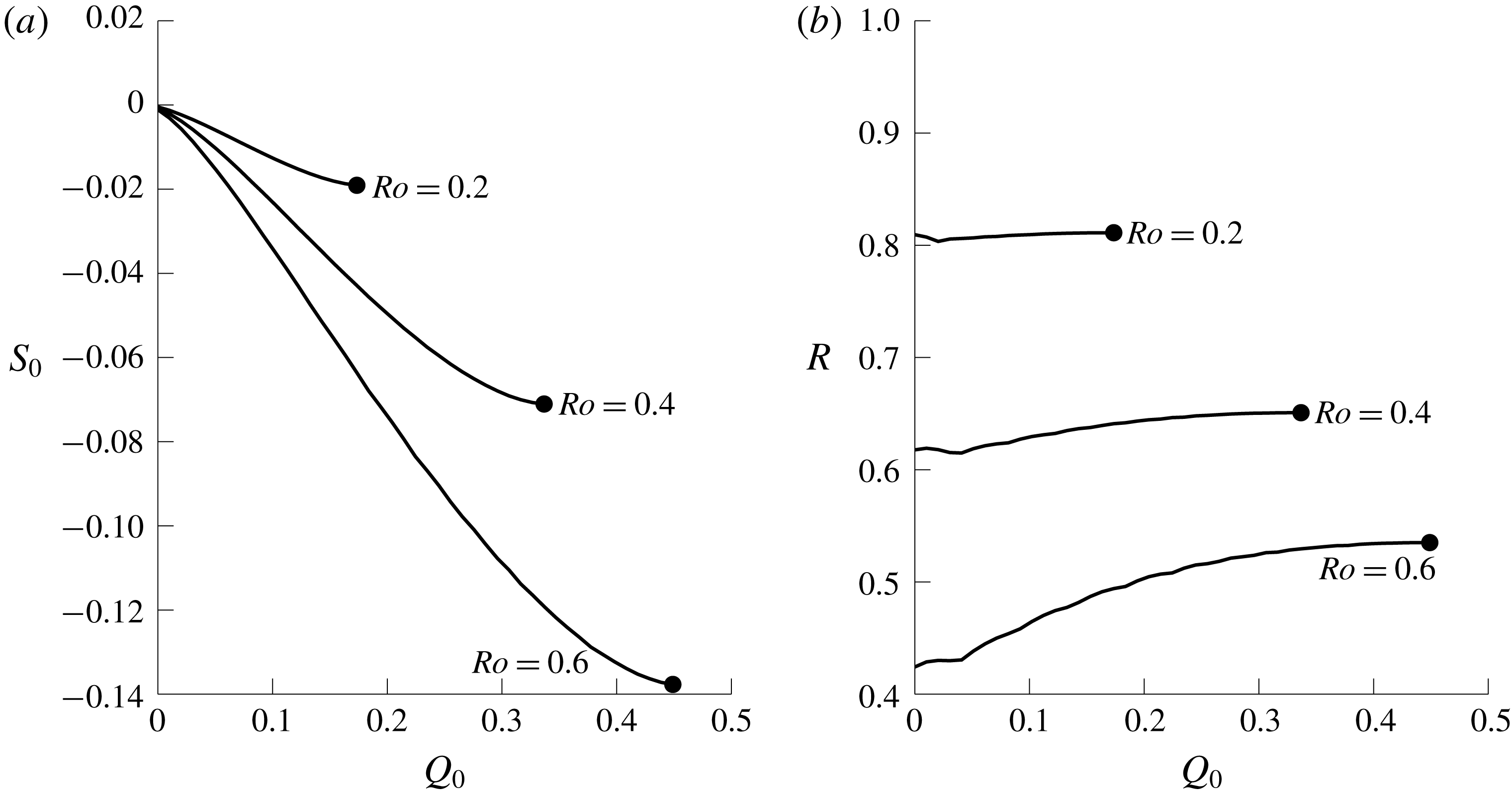
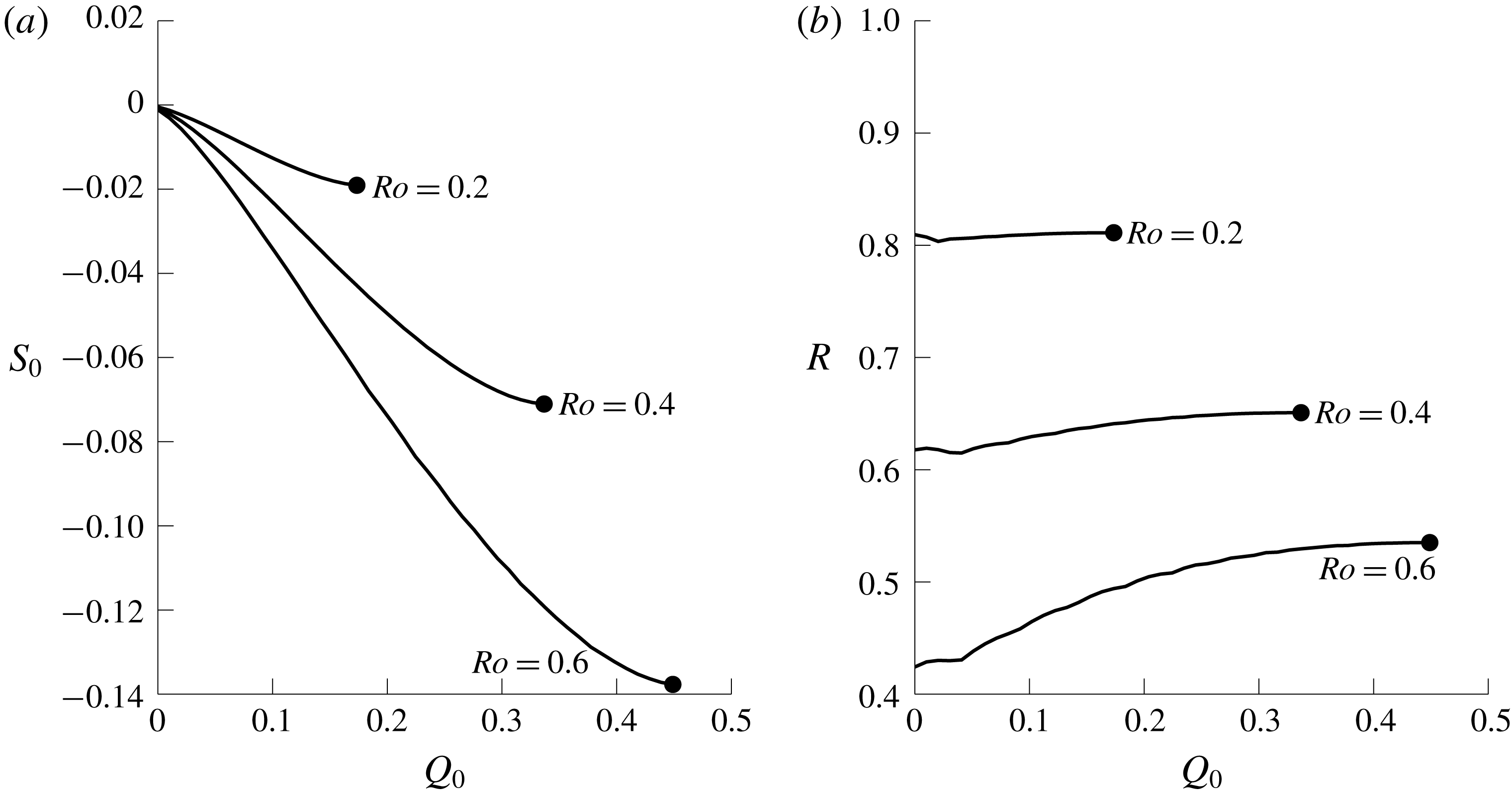
Figure 15 shows both
 $S_{0}$
and
 $R$
for various steady solutions. For small
 $Ro$
or
 $Q_{0}$
,
 $R\approx H$
, replicating the result for positive PVa. The momentum flux
 $|S_{0}|$
increases with the volume flux
 $Q_{0}$
, with larger
 $Ro$
corresponding to larger momentum flux.
Constants of motion for steady solutions with negative PVa. (a) The momentum injected by the source,
 $S_{0}$
. (b) The total energy
 $R$
.
4.3 Downstream rarefaction
Once the steady solution has been determined, analysis via Riemann invariants can be applied by integrating (3.12) away from the point
 $U(w_{D})=U_{c}$
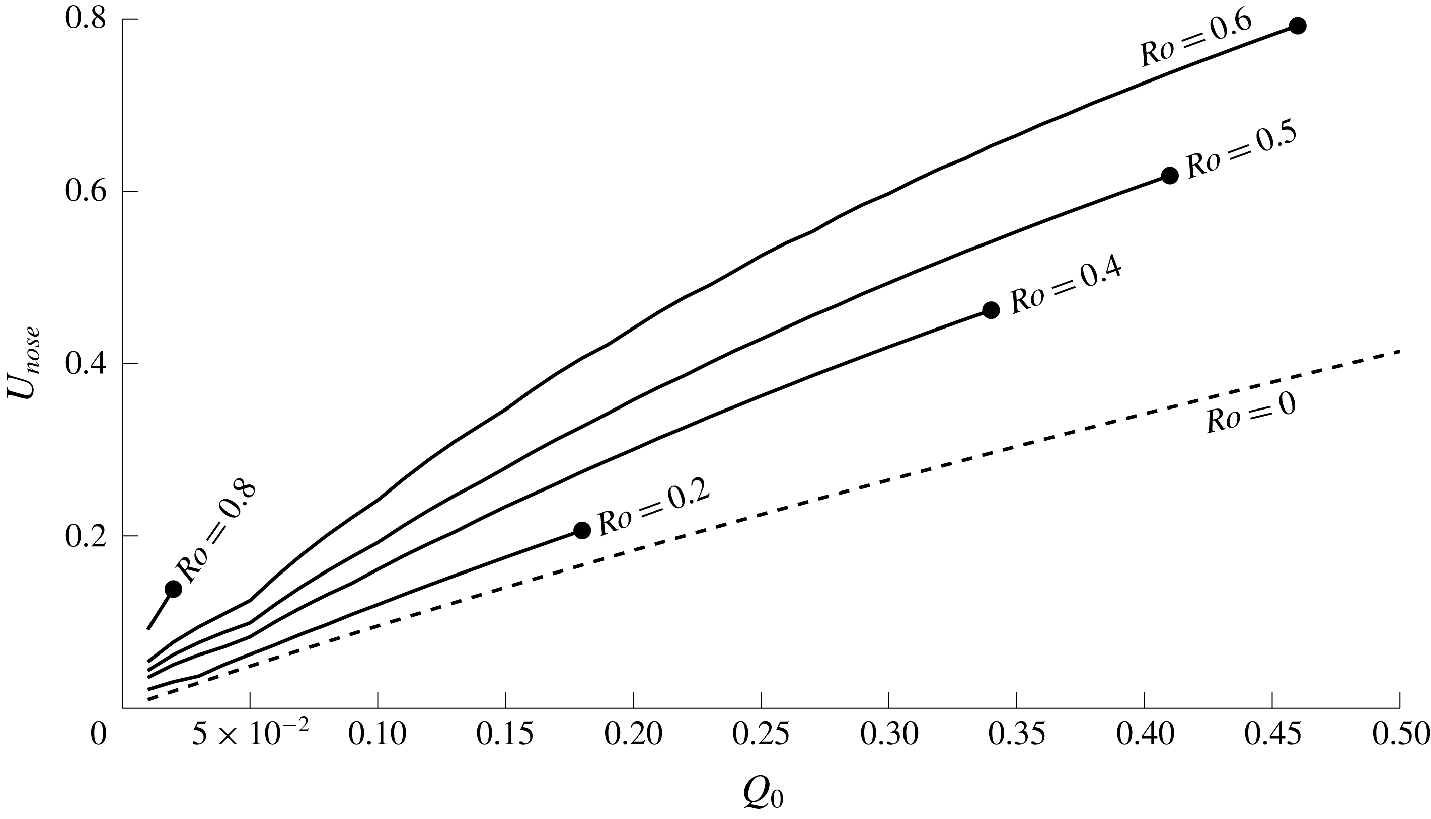
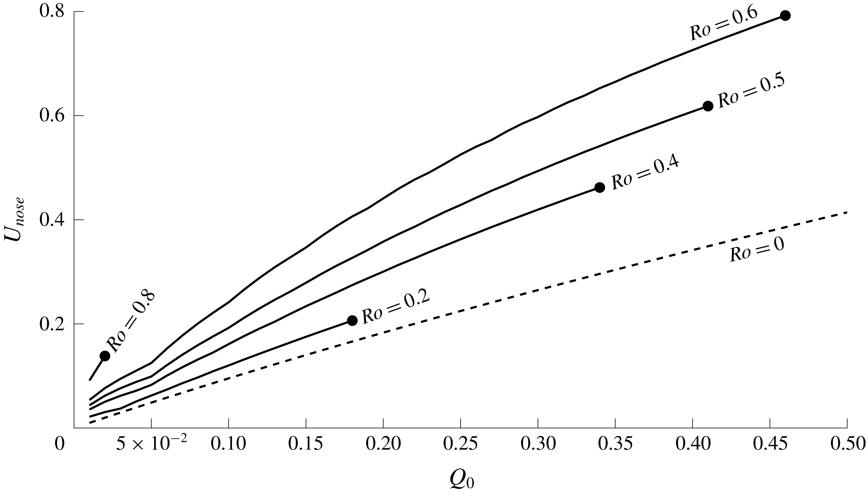
. In particular, figure 16 shows
 $U_{nose}$
as a function of
 $Q_{0}$
for various
 $Ro$
, allowing direct comparison with figure 10. As with positive PVa, increasing the mass flux for a fixed
 $Ro$
increases the nose speed. However, in contrast to figure 10, fixing
 $Q_{0}$
and increasing
 $Ro$
now increases the nose speed. That is, the fluid speed in the nonlinear Kelvin wave becomes slower and slower as the outer-layer depth is decreased, irrespective of the sign of the PVa. A similar relationship between
 $U_{nose}$
and layer depth is shown in Stern & Helfrich (Reference Stern and Helfrich2002, figure 2), and in Martin, Smeed & Lane-Serff (Reference Martin, Smeed and Lane-Serff2005, figure 3). The thin dashed horizontal line in figure 12(b) shows the value of
 $U_{nose}$
predicted from the analysis of the Riemann invariants, and is in good agreement with the numerical solution. When the current width vanishes, i.e.
 $w=0$
, the characteristic speed
 $\unicode[STIX]{x1D706}_{R}$
reduces to
 $U$
and so, since the rarefaction joins smoothly to the coast,
 $U_{nose}$
is also the propagation velocity of the expelled fluid at the farthest downstream edge. This is confirmed by the two vertical lines in figure 12(a), which are separated by
 $20U_{nose}$
corresponding to the interval between solutions at
 $t=20$
and
 $t=40$
.
The nose speed
 $U_{nose}$
for a controlled rarefaction, as a function of
 $Q_{0}$
. The dashed line shows the wall velocity of the zero PVa solution.
The upstream rarefaction for steady solutions with negative PVa can also be described by Riemann invariants, although in this case it is
 ${\mathcal{R}}_{R}$
that is uniform. Applying a similar test to (3.13) shows that a shock always forms upstream for negative PVa, and the same ideas about matching shock and characteristic velocities can be used to determine the maximum width of this, which increases as vortical effects become more important.
4.4 Range of behaviours for negative PVa
For negative PVa, solutions can be categorised according to whether they are steady in the source region. In the quasi-geostrophic limit, JSM found that the speed ratio
 $a$
was again of crucial importance, with
 $a>1$
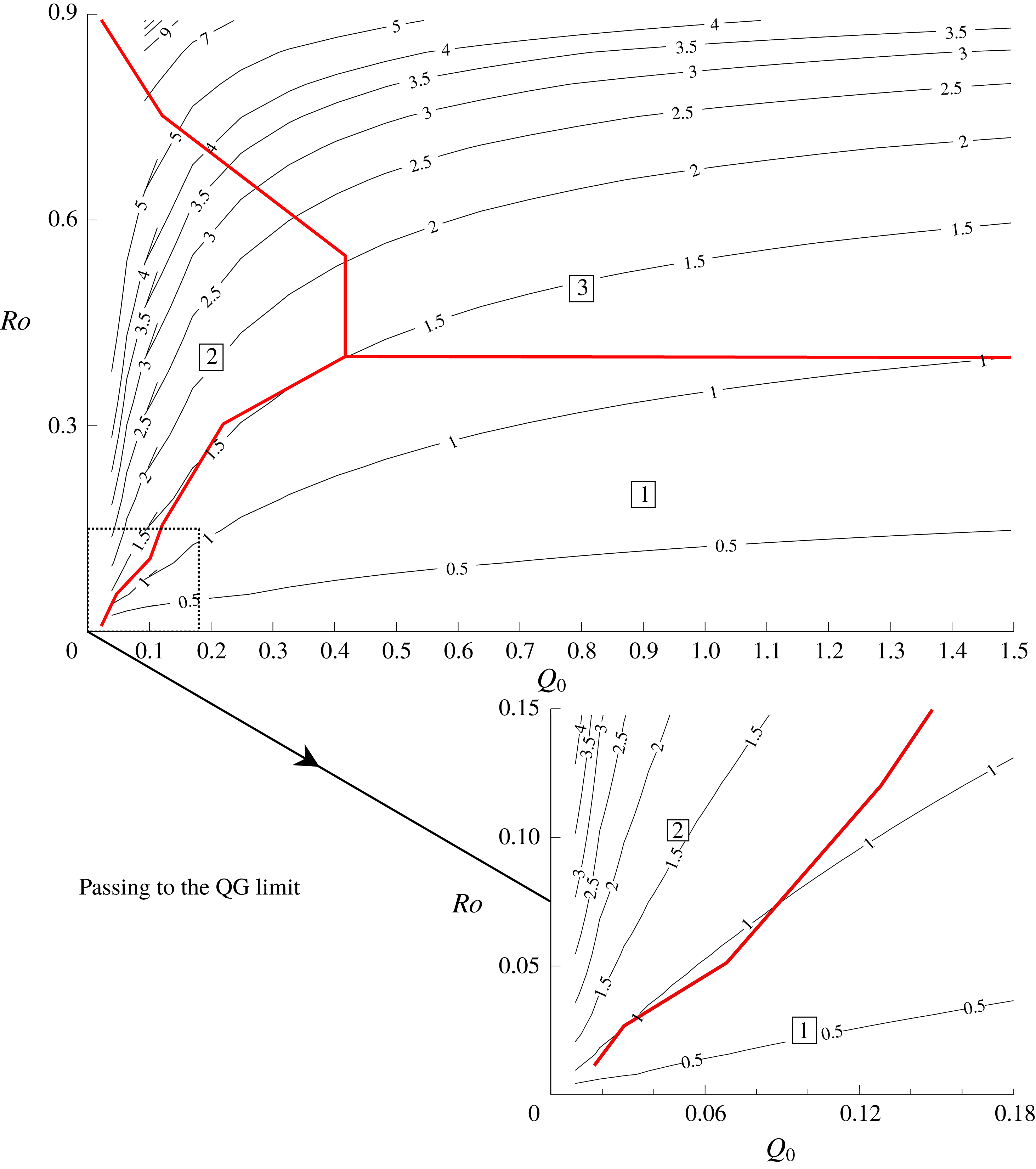
being necessary for a steady solution to form. Figure 17 shows the type of solution that occurs in semi-geostrophic flow based on the values of the two physical parameters
 $Ro$
and
 $Q_{0}$
. The solution type was determined by attempting to compute a steady solution that satisfies both (4.1) and (4.3). If, for a given
 $Q_{0}$
and
 $Ro$
, such a solution is possible, then these values permit a steady solution (region two). A fine sweep of the quasi-geostrophic limit of small
 $Q_{0}$
and
 $Ro$
shows that the boundary between flows that are steady and those that grow (region one) aligns with the contour
 $a=1$
as expected. In addition to this test, which is based on the asymptotic theory of § 4.2, the initial-value problem was solved over the full parameter range, using a grid that was refined close to the apparent boundaries between regions. Although there were some quantitative differences between theoretical and numerical results (these being larger far away from the QG limit) the test based on (4.3) and (4.1) was found to correctly describe the qualitative behaviour of all solutions.
Solution type for negative PVa, compared with curves of constant speed ratio
 $a$
. Solution type one grows indefinitely in the source region, solution type two is steady and solution type three is believed to separate from the wall. The inset shows that the boundary between regions one and two aligns with the curve
 $a=1$
in the quasi-geostrophic limit.
As for positive PVa, away from the quasi-geostrophic limit region boundaries can differ from contours of
 $a$
, and so the system depends on
 $Q_{0}$
and
 $Ro$
independently, although it is still the case that solutions with small
 $a$
(Kelvin-wave dominated) are of the growing type. The shape of region two reflects the results of figure 14(a), where increasing
 $Ro$
allows a larger flux to be supported by steady solutions until, at some cut-off point around
 $Ro=0.6$
, the maximum permitted flux starts to decrease again. Increasing
 $Ro$
past this point is associated with a rapid increase in the value of
 $a$
– for flows that are strongly dominated by vorticity, steady solutions occur only at small fluxes.
Parameter values in the region marked ‘3’ in figure 17 give rise to complex solutions to (4.1) and (4.3). It appears that as the current width grows, the coastal layer depth
 $h_{W}$
decreases to zero and the expelled fluid separates from the coast. For negative
 $u$
,
 $\unicode[STIX]{x2202}h/\unicode[STIX]{x2202}y$
is positive and the expelled fluid is shallower at the coast than immediately offshore. If the initial outer layer depth is small (large
 $Ro$
) and the magnitude of the wall velocity is sufficiently large, this suggests that the layer depth shrinks to zero and the expelled fluid is no longer attached to the coast upstream of the source.
Separation is explicitly excluded from the model presented here by the assumption that the expelled fluid lies in
 $0<y<w$
. Preliminary results from adapting the model to remove this restriction suggest that the fluid tries to separate in the source region, as discussed for separated flow out of a basin in, for example, Gill (Reference Gill1977) and Helfrich et al. (Reference Helfrich, Kuo and Pratt1999), as well as for laboratory experiments in Horner-Devine et al. (Reference Horner-Devine, Fong, Monismith and Maxworthy2006). For the present model, separation in the source region modifies the outflow profile
 $Q(x)$
and thus alters the problem beyond the scope considered here.
If for a given
 $Q_{0}$
and
 $Ro$
the solution starts to separate (
 $h_{W}=0$
), the initial-value problem is halted and the parameter pair is included in region three. It appears that the boundary between solutions which grow and those which separate is sharp in terms of
 $Ro$
: if the Rossby number is increased beyond some critical value of
 $Ro\approx 0.4$
then all unsteady flows eventually separate from the wall.
5 Discussion
Numerical and theoretical results for coastal outflows have been discussed using a semi-geostrophic model that allows for large variations in Rossby number by adjusting the depth of the outer buoyant ocean layer. For positive PVa (when the depth of the buoyant layer is greater than the potential vorticity depth of the river water) a full theory has been developed based on numerically computed Riemann invariants, while for negative PVa an asymptotic theory for solutions that are steady across the source region is derived. The speed ratio
 $a$
, which measures the relative strengths of Kelvin-wave flow and image vorticity, is a useful guide to determining the behaviour of the outflow. However, for moderate and larger Rossby number, solutions depend on both
 $Ro$
and the total mass flux
 $Q_{0}$
independently. Diagrams describing the behaviour of the solutions for a given
 $Q_{0}$
and
 $Ro$
are presented for positive PVa in figure 9, and for negative PVa in figure 17.
For positive PVa, the range of possible behaviours is the same as in the quasi-geostrophic limit of JSM. All currents flow exclusively downstream, are steady across the source region, and are led by a rarefaction that either joins smoothly to the wall or develops a shock in finite time. The key feature here, however, is that the Kelvin wave that propagates ahead of the expelled fluid does so at a finite speed. The speed of the fluid within the Kelvin wave,
 $U_{nose}$
, is found to be greater when the depth of the outer layer is shallower. The propagation speed of the Kelvin wave is given as
 $V_{KW}$
in (3.18), while the propagation speed of the expelled fluid can be computed from (3.16) using the maximum values of
 $w$
and
 $U$
just behind the shock. The ability to measure the fluid and propagation speeds of these two waves separately is a key feature of this work, and the way that these quantities vary with the parameters, along with the range of behaviours observed, highlights the importance of vortical turning in determining how the outflow behaves. It is also important to note that most experiments on outflows use colouring to identify the expelled fluid, and thus tend to report on disturbances only within this coloured region, leaving laboratory investigation of the nonlinear Kelvin wave in the outflow problem as an avenue for future work.
For negative PVa, steady and growing solutions exist as in the quasi-geostrophic limit, with steady solutions occurring in cases where the vortical flow is stronger than the Kelvin-wave-driven flow. However, for large
 $Ro$
(shallow oceanic layers) sufficiently strong forcing can cause the flow to separate away from the wall – a phenomenon that has been previously noticed when studying related flows and one that remains to be explored further in the present context. The steady solutions obtained here are critically controlled at the downstream edge of the source: the phase speed of all long-wave disturbances is positive in
 $x>1$
, so the flow here is supercritical, while in
 $x<1$
long-wave disturbances can propagate in either direction and the flow is subcritical. All fluid first heads upstream along the wall, before a portion of it recirculates and re-crosses the source region. This creates an anti-cyclonic circulation within and upstream of the river mouth, as in the density-driven solutions of McCreary et al. (Reference McCreary, Zhang and Shetye1997), the numerical results of Isobe (Reference Isobe2005) and the laboratory experiments of Avicola & Huq (Reference Avicola and Huq2003) and Thomas & Linden (Reference Thomas and Linden2007). That similar qualitative behaviours are observed here as in the experiments supports an analogy between PV jumps and density fronts previously alluded to in McCreary et al. (Reference McCreary, Zhang and Shetye1997), and possibly suggests that both mechanisms contribute to offshore plumes observed in the oceans.
One factor that has not been discussed here is the role played by a sloping coastline, which allows for the possibility of buoyant outflows that remain attached to the sea floor (‘bottom-advected plumes’). According to Yankovsky & Chapman (Reference Yankovsky and Chapman1997), surface-advected plumes (those which do not touch the bottom) occur when
 $2L_{0}v_{0}f/g^{\prime }<h_{0}$
, where
 $L_{0}$
and
 $h_{0}$
are the width and depth of the river mouth, and
 $v_{0}$
is the velocity of fluid as it enters the ocean. The model developed above has a vertical coast and so excludes bottom advection, but it seems plausible that a surface-advected plume above a sloping coastline behaves similarly to a plume against a vertical coastline.
The photograph of the Elwha river after dam removal (figure 1) bears a striking similarity to solutions with positive PVa (figures 3, 4). Although the outflow after the dam was dismantled involved the expulsion of sediment-laden river water (and so differs from the homogeneous density model considered here) it is evident from figure 1 that there was a strong downstream transport of river water, with a qualitatively similar shape to the positive PVa solutions of § 3. Juan de Fuca – the strait into which the Elwha river runs – is an important shipping route, and as such there is much data available that explores the oceanography of the region. A comprehensive survey conducted between 1975 and 1980 (well before the dam was removed) shows that most of the time the prevailing currents and tides carry surface fluid towards the sea, which is leftward to an observer facing the ocean (Cannon Reference Cannon1978; Holbrook et al. Reference Holbrook, Muench, Kachel, Wright, Klutznick, Frank and Hess1980; Holbrook & Halpern Reference Holbrook and Halpern1982). Although up-strait flow does occur, it is comparatively rare and weak and is thus unlikely to be the sole cause of the rightward turning in figure 1. Finally, technical data from Curran et al. (Reference Curran, Konrad, Dinehart and Moran2008) suggests that the outflow after dam removal satisfies the condition of Yankovsky & Chapman (Reference Yankovsky and Chapman1997) and so should not be strongly affected by bottom advection.
The present model focuses on the role of PVa in the outflow problem by assuming that the expelled fluid and the buoyant ocean layer have the same density. This is rarely, if ever, true in an ocean setting where horizontal buoyancy gradients also play a role in the formation and propagation of coastal currents, and so direct applicability of the model to a real ocean is limited. On the other hand, the two mechanisms of vortex stretching and Kelvin-wave-driven flow described in this work are still present, and in the limit of weak horizontal stratification it is possible that they are the dominant dynamical factors. It is also plausible that buoyancy effects are restricted to a region around the density front (Sher & Woods Reference Sher and Woods2017) (see figure 18 and discussion below). Further theoretical exploration of how buoyancy interacts with the two effects considered here remains an important avenue for future work.
Comparison between numerical results from the present model with
 $H=0.4$
,
 $Q_{0}=0.53$
(dashed curve, red online) and laboratory experiment VB6 from Horner-Devine et al. (Reference Horner-Devine, Fong, Monismith and Maxworthy2006) (solid curve, black online). The dimensional along-shore velocity
 $u^{\ast }$
is shown as a function of the off-shore coordinate
 $y^{\ast }$
. The transect is taken at the mid-point between the downstream edge of the source and the upstream edge of the expelled fluid, and so intersects the centre of the bulge, at the time
 $t=30$
. The horizontal dashed line gives
 $w$
at this value of
 $x$
and
 $t$
.
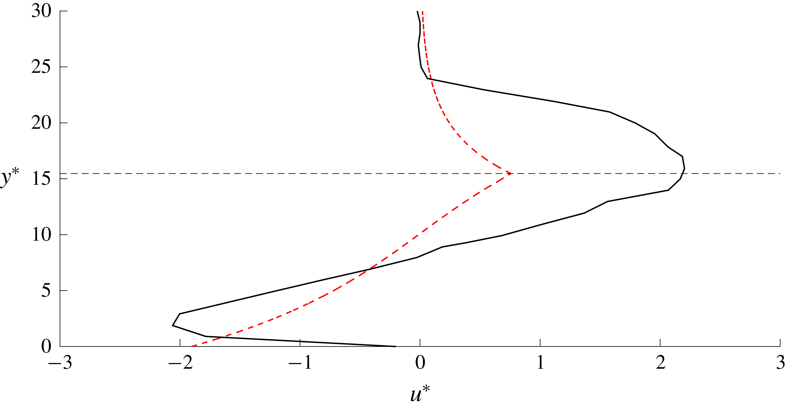
Horner-Devine et al. (Reference Horner-Devine, Fong, Monismith and Maxworthy2006) studied the injection of fluid (assumed to have zero PV) into a rotating annulus of uniform, denser fluid, and their results are therefore most comparable to our model with small
 $H$
(large negative PVa). Indeed, they find a bulge in the source region and a thinning current that propagates downstream. Figure 18 makes a quantitative comparison of dimensional
 $u^{\ast }$
from our model with that from their experiments, in an off-shore transect that intersects the bulge centre (the green dashed line in figure 12
a). Non-dimensionalising their experimental values gives a mass flux
 $Q_{0}=0.53$
, and so our model predicts unsteady flow in the source region for all
 $H$
. JSM show that in the QG limit, the growth of the current width
 $\unicode[STIX]{x2202}w/\unicode[STIX]{x2202}t$
is proportional to
 $1/t$
for unsteady solutions, and so the flow is approximately steady at large
 $t$
. The best comparison between our theory and the results of Horner-Devine et al. (Reference Horner-Devine, Fong, Monismith and Maxworthy2006) is therefore made by taking the smallest
 $H$
for which the flow remains attached to the coast sufficiently long to become approximately steady. The choice of
 $H=0.4$
allows the integration to run until
 $t=80$
, and tests with other values of
 $H$
show that the quantitative behaviour is remarkably unaffected. The flow within the bulge is bi-directional, with fluid closer to the wall travelling upstream under the influence of image vorticity – something that is only possible when the source fluid has lower PV than the oceanic fluid. There is excellent agreement between the wall velocity of the model and the near-wall velocity observed in the experiment, and both the predicted and the observed velocities increase until they reach a maximum value at a similar off-shore coordinate (which occurs at the PV jump in our results, and the edge of the bulge in the laboratory experiment) before decaying back to zero. As
 $H\rightarrow 0$
,
 $a\rightarrow \infty$
and the vortical length scale
 $L_{v}\rightarrow 0$
, so we expect that vortical effects will only be felt close to the wall. Indeed the agreement between the numerical results and the experiment is best closer to the coast and the largest discrepancies occur further offshore, where the differences in set-up between the experiment and the model are more significant.
Appendix A. Eigenvalues and Riemann invariants
A.1 Expressions for
$\unicode[STIX]{x1D706}$
and
$\unicode[STIX]{x1D6FC}_{C/R}$


The governing equations (2.12) and (2.13) are diagonalised and hence recast in the form
 $$\begin{eqnarray}\frac{\unicode[STIX]{x2202}}{\unicode[STIX]{x2202}t}\binom{U}{w}+\frac{1}{a+b}\left(\begin{array}{@{}cc@{}}c+b(U+\sqrt{H}) & d\\ c-a(U+\sqrt{H}) & d\end{array}\right)\frac{\unicode[STIX]{x2202}}{\unicode[STIX]{x2202}x}\binom{U}{w}=\frac{Q^{\prime }(x)}{a+b}\binom{1}{1},\end{eqnarray}$$
where
 $$\begin{eqnarray}\displaystyle & \displaystyle a=-1+H+\cosh w+\sqrt{H}\sinh w, & \displaystyle\end{eqnarray}$$
 $$\begin{eqnarray}\displaystyle & \displaystyle b=(H-1)(-1+\cosh w)+(\sqrt{H}\cosh w+\sinh w)U, & \displaystyle\end{eqnarray}$$
 $$\begin{eqnarray}\displaystyle & \displaystyle c=(\sqrt{H}\cosh w+\sinh w)(1+U\sinh w+\cosh w(-1+H+\sqrt{H}U)), & \displaystyle\end{eqnarray}$$
 $$\begin{eqnarray}\displaystyle & \displaystyle d=((H-1)\sinh w+U(\cosh w+\sqrt{H}\sinh w)) & \displaystyle \nonumber\\ \displaystyle & \displaystyle \hphantom{dd\times =}\times \,(1+U\sinh w+\cosh w(-1+H+\sqrt{H}U)), & \displaystyle\end{eqnarray}$$
which leads to the eigenvalues
 $$\begin{eqnarray}\displaystyle \unicode[STIX]{x1D706}_{\pm } & = & \displaystyle \frac{1}{2(a+b)} (\!c+d+b(U+\sqrt{H})\nonumber\\ \displaystyle & & \displaystyle \pm \sqrt{(-4d(a+b)(U+\surd H)+(c+d+b(U+\surd H))^{2})}\!).\end{eqnarray}$$
Outside the source region, the right-hand side of (A 1) is homogenous and so there exist left eigenvectors
 $\boldsymbol{k}_{\pm }$
such that
 $$\begin{eqnarray}\boldsymbol{k}_{\pm }^{T}\left(\frac{\unicode[STIX]{x2202}}{\unicode[STIX]{x2202}t}\binom{U}{w}+\unicode[STIX]{x1D706}_{\pm }\frac{\unicode[STIX]{x2202}}{\unicode[STIX]{x2202}x}\binom{U}{w}\right)=0,\end{eqnarray}$$
or,
 $$\begin{eqnarray}k_{\pm ,1}\frac{\text{d}U}{\text{d}t}+k_{\pm ,2}\frac{\text{d}w}{\text{d}t}=0\quad \text{on }\frac{\text{d}x}{\text{d}t}=\unicode[STIX]{x1D706}_{\pm },\end{eqnarray}$$
or
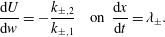 $$\begin{eqnarray}\frac{\text{d}U}{\text{d}w}=-\frac{k_{\pm ,2}}{k_{\pm ,1}}\quad \text{on }\frac{\text{d}x}{\text{d}t}=\unicode[STIX]{x1D706}_{\pm }.\end{eqnarray}$$
These are the ODEs that determine the Riemann invariants as described in (3.11). The eigenvectors
 $\boldsymbol{k}$
can always be chosen so that
 $k_{\pm ,2}=1$
, in which case
 $$\begin{eqnarray}\displaystyle & \displaystyle \frac{\text{d}U}{\text{d}w}=-\frac{d}{\unicode[STIX]{x1D706}_{\pm }(a+b)}\left(\frac{\unicode[STIX]{x1D707}_{\pm }+d}{\unicode[STIX]{x1D707}_{\pm }-d}\right)=\unicode[STIX]{x1D6FC}_{C/R}, & \displaystyle\end{eqnarray}$$
 $$\begin{eqnarray}\displaystyle & \displaystyle \unicode[STIX]{x1D707}_{\pm }=c+b(U+\sqrt{H})\hphantom{-4d(a+b)(U+\surd H)+(c+d)}\qquad & \displaystyle \nonumber\\ \displaystyle & \displaystyle \hphantom{-4d(a+b)}\pm \sqrt{(-4d(a+b)(U+\surd H)+(c+d+b(U+\surd H))^{2})}.\qquad & \displaystyle\end{eqnarray}$$
A.2 Values of
$\unicode[STIX]{x1D706}$
in various limits

Note that
 $$\begin{eqnarray}a+b=(\sqrt{H}\cosh w+\sinh w)(\sqrt{H}+U)\end{eqnarray}$$
which is positive, subject to the observation that
 $w$
and
 $U$
are non-negative in all solutions here. Thus, from (A 6), we can define
 $\unicode[STIX]{x1D706}_{C}=\unicode[STIX]{x1D706}_{+}$
and
 $\unicode[STIX]{x1D706}_{R}=\unicode[STIX]{x1D706}_{-}$
with
 $\unicode[STIX]{x1D706}_{C}\geqslant \unicode[STIX]{x1D706}_{R}$
always, and from now on it is only necessary to consider the numerator when checking the sign of
 $\unicode[STIX]{x1D706}_{C/R}$
.
Further, taking
 $w=0$
gives the following:
 $$\begin{eqnarray}[a,b,c,d]=[H,\sqrt{H}U,H(U+\sqrt{H}),\sqrt{H}U(U+\sqrt{H})],\end{eqnarray}$$
so that the numerator in (A 6) simplifies to
 $$\begin{eqnarray}(2U+\sqrt{H})(U+\sqrt{H})\pm H(\sqrt{H}+U)=(2U+\sqrt{H}\pm H)(\sqrt{H}+U),\end{eqnarray}$$
which gives
 $\unicode[STIX]{x1D706}_{R}=U$
and
 $\unicode[STIX]{x1D706}_{C}=U+\surd H$
. Thus when additionally
 $U=0$
,
 $\unicode[STIX]{x1D706}_{R}=0$
and
 $\unicode[STIX]{x1D706}_{C}=\surd H$
.
The repetition of terms in the numerator of
 $\unicode[STIX]{x1D706}_{C/R}$
shows that
 $\unicode[STIX]{x1D706}_{C/R}=0$
only when
 $$\begin{eqnarray}-4d(a+b)(U+\sqrt{H})=0\end{eqnarray}$$
with
 $\unicode[STIX]{x1D706}_{R}=0$
if
 $c+d+b(U+\surd H)>0$
and
 $\unicode[STIX]{x1D706}_{C}=0$
otherwise. Equation (A 15) is satisfied only if
 $d=0$
, or equivalently if one of
 $$\begin{eqnarray}\displaystyle & \displaystyle (H-1+\sqrt{H}U)\sinh w+U\cosh w=0, & \displaystyle\end{eqnarray}$$
 $$\begin{eqnarray}\displaystyle & \displaystyle (H-1+\sqrt{H}U)\cosh w+U\sinh w=-1 & \displaystyle\end{eqnarray}$$
holds. But, from (2.8) and (2.10) this requires that either
 $u_{W}=0$
or
 $h_{W}=0$
. The latter is forbidden in the model used here, and setting
 $u_{W}=0$
gives
 $$\begin{eqnarray}c+d+b(U+\sqrt{H})=(\sqrt{H}\cosh w+\sinh w)(U+\sqrt{H})^{2}\end{eqnarray}$$
which is always positive. Hence
 $\unicode[STIX]{x1D706}_{C}$
is never zero, and since
 $\unicode[STIX]{x1D706}_{C}$
is positive when
 $t=0$
it must remain so for
 $t>0$
. Further,
 $\unicode[STIX]{x1D706}_{R}=0$
for
 $t>0$
is equivalent to
 $u_{W}=0$
, a constraint which is physical only if
 $H<1$
. Thus,
 $\unicode[STIX]{x1D706}_{R}$
cannot change sign in outflows with positive PVa. Expanding for small
 $w$
and
 $U$
gives
 $$\begin{eqnarray}\unicode[STIX]{x1D706}_{R}\sim U+(H-1)w\quad \text{as }U\rightarrow 0,w\rightarrow 0\end{eqnarray}$$
so that
 $\unicode[STIX]{x1D706}_{R}>0$
initially, and hence always, when
 $H>1$
.