1 Introduction
Energy conversion devices with high power densities, such as gas turbines, can exhibit thermo-acoustic instabilities (Lieuwen & Yang Reference Lieuwen and Yang2005; Culick & Kuentzmann Reference Culick and Kuentzmann2006), caused by a resonant feedback between acoustic radiation and combustion processes (Candel Reference Candel1992; Dowling Reference Dowling1995; Sattelmayer & Polifke Reference Sattelmayer and Polifke2003). The driving mechanism behind such instabilities was recognized by Lord Rayleigh (1878) who observed amplifying oscillations when pressure and heat-release fluctuations were in phase and caused positive feedback effects.
Thermo-acoustic instabilities severely affect the lifetime, performance and operational safety of energy conversion devices. In an effort to meet reduced mono-nitrogen oxide (
 $\text{NO}_{x}$
) and soot emissions mandated by environmental regulatory policies, high-performance engines often operate in the lean regime, where thermo-acoustic instabilities prevail (Harrje Reference Harrje1972; Culick Reference Culick1989). The additional absence of bypass air in convectively cooled combustion systems yields a decrease of acoustic damping and an increase in pulsation amplitudes, further increasing the likelihood of instability. Hence, a combination of lean-burn parameters and convectively cooled combustion chambers has made energy conversion devices more prone to combustion-driven oscillations, or thermo-acoustic instabilities. These oscillations typically trigger the lowest-frequency eigenmodes (Sensiau, Nicoud & Poinsot Reference Sensiau, Nicoud and Poinsot2008). As the radial and longitudinal dimensions of most combustion chambers are shorter than their azimuthal dimension, these lowest-frequency modes manifest themselves as azimuthal modes (Salas Reference Salas2013).
Experimental investigations on full-scale engines are difficult and expensive (Poinsot et al. Reference Poinsot, Trouve, Veynante, Candel and Esposito1987; Lee & Anderson Reference Lee and Anderson1999; Lee & Lieuwen Reference Lee and Lieuwen2003). Therefore, simplified configurations have been used to study both longitudinal and azimuthal instabilities. Earlier studies by Candel et al. (Reference Candel, Maistret, Darabiha, Poinsot, Veynante and Lacas1988), Candel, Durox & Schuller (Reference Candel, Durox and Schuller2004) and Ducruix et al. (Reference Ducruix, Schuller, Durox and Candel2005) focused on longitudinal combustion instabilities, while, more recently, azimuthal modes were studied in a simplified, annular Rijke-tube configuration, using heating grids as the unsteady heat source (Moeck, Paul & Paschereit Reference Moeck, Paul and Paschereit2010; Gelbert et al. Reference Gelbert, Moeck, Paschereit and King2012). Worth & Dawson (Reference Worth and Dawson2013a ,Reference Worth and Dawson b ) examined an annular configuration with swirled, premixed flames to study the interaction between the flames and the mean swirl as well as changes to the stability and nature of azimuthal modes. However, swirling turbulent flames can compromise the study of the thermo-acoustic phenomena; therefore, Bourgouin et al. (Reference Bourgouin, Durox, Moeck, Schuller and Candel2015) specifically designed an annular combustion chamber to avoid such complexities. It is worth mentioning that the effects of turbulence are difficult to incorporate into a deterministic model such as the one presented here (Noiray, Bothien & Schuermans Reference Noiray, Bothien and Schuermans2011); however, Noiray & Schuermans (Reference Noiray and Schuermans2013) have explained how real gas-turbine data and theoretical predictions can be reconciled by including into the model stochastic forcing terms accounting for combustion noise. Experiments of this type provide invaluable insight, but require significant cost and effort (Dowling Reference Dowling1995; Kopitz et al. Reference Kopitz, Huber, Sattelmayer and Polifke2005; Nicoud & Poinsot Reference Nicoud and Poinsot2005), motivating analytical and numerical approaches, ranging from theoretical models, via low-order network methods, to full-scale large eddy simulations (LES). The cost and complexity of each approach increases with the level of fidelity and detailed insight it provides.
Three-dimensional numerical simulations, such as LES, are capable of reproducing combustion instabilities in complex geometries by accounting for the relevant mechanisms with minimal modelling assumptions. Recent studies by Staffelbach et al. (Reference Staffelbach, Gicquel, Boudier and Poinsot2009) or Wolf et al. (Reference Wolf, Staffelbach, Gicquel, Müller and Poinsot2012) have successfully simulated azimuthal instabilities in real gas-turbine combustion chambers using LES. Although computationally demanding, LES can predict and reproduce combustion instabilities, but can provide only limited insight into means to identify and control the unstable modes that arise (Dowling Reference Dowling1995; Kopitz et al. Reference Kopitz, Huber, Sattelmayer and Polifke2005; Nicoud & Poinsot Reference Nicoud and Poinsot2005). Hence, low-order and low-complexity models are needed to guide computationally intensive simulations or experiments.
The need to investigate combustion processes across multiple, varying parameters, to determine the manner in which they affect instabilities, and to explore potential control strategies, has generated renewed interest in analytical techniques (Clavin, Pelcé & He Reference Clavin, Pelcé and He1990; Dowling Reference Dowling1995; Poinsot & Veynante Reference Poinsot and Veynante2005), where the nature and structure of azimuthal modes in annular combustion chambers have been clarified without computational simulations (Parmentier et al. Reference Parmentier, Salas, Wolf, Staffelbach, Nicoud and Poinsot2012). Using simple geometric configurations, studies of this kind provide a mechanistic point of view and guide the interpretation of thermo-acoustic instabilities in more complex simulations. However, these methods rely on hypotheses that have to be satisfied in order to simplify the problem; hence only configurations and geometries of low complexity can be studied.
Network models can be used to explore moderately complex geometries and configurations, where analytical studies fail. Using this approach, the actual geometry is decomposed into a set of lumped acoustic elements and compact heat sources. Each element is modelled by means of a linear transfer function (Polifke, Paschereit & Döbbeling Reference Polifke, Paschereit and Döbbeling2001; Stow & Dowling Reference Stow and Dowling2001; Poinsot & Veynante Reference Poinsot and Veynante2005) and composed into a more complex system. In a recent investigation by Parmentier et al. (Reference Parmentier, Salas, Wolf, Staffelbach, Nicoud and Poinsot2012), a semi-analytical approach with a one-dimensional network model was used to study azimuthal modes in a single ring configuration. In Bauerheim et al. (Reference Bauerheim, Parmentier, Salas, Nicoud and Poinsot2014), this model was extended to a coupled set of one-dimensional networks for the analysis of two-ring configurations. The network approach is computationally efficient and allows for phenomenological interpretation of thermo-acoustic instabilities within the limits of moderately complex geometries.
In situations where more complex and detailed effects need to be accounted for, such as the response of a spatially distributed flame, the one-dimensional propagation models must be replaced by the multi-dimensional wave equation, often formulated as a Helmholtz problem. In a recent study by Mensah & Moeck (Reference Mensah and Moeck2015), a thermo-acoustic model based on the Helmholtz equation was used to exploit the discrete rotational symmetry, common to most energy conversion devices, and to isolate special solutions of so-called Bloch type. These solutions are obtained by considering a single representative segment of the geometry, with the appropriate Bloch-type boundary conditions, creating an
 $N$
-periodic geometry, significantly reducing the computational effort required to determine the eigenstructure of the full system. The Bloch-wave formalism supports the appropriate boundary conditions that account for the influence of adjacent periodic elements along the azimuthal direction whilst constructing all possible, globally periodic modes of the full system (and thus the large-scale dynamics of the entire system). Mathematically, this technique is equivalent to the framework employed in this article (although we prefer a time-domain formulation as proposed in Schmid, de Pando & Peake (Reference Schmid, Fosas de Pando and Peake2017)). In light of the inherently azimuthal and non-normal nature of the unstable modes of
 $N$
-periodic systems (Mariappan, Sujith & Schmid Reference Mariappan, Sujith and Schmid2011; Sujith, Juniper & Schmid Reference Sujith, Juniper and Schmid2016; Balasubramanian & Sujith Reference Balasubramanian and Sujith2008, Reference Balasubramanian and Sujith2013), this article focuses on the manner in which unsteady pressure in the chamber (azimuthal modes) can lead to unsteady flow rates within the burners, and thus couple the burner elements of an
 $N$
-periodic energy conversion device into synchronized groups.
A physical motivation for this study is given by the observation of azimuthal structures, especially rotating structures, in annular combustion chamber geometries. In order to model this trans-unit interaction phenomenon we consider a dynamical system consisting of one-dimensional burner elements coupled via a one-dimensional chamber and plenum network. This geometry is similar to the one presented in Bauerheim et al. (Reference Bauerheim, Parmentier, Salas, Nicoud and Poinsot2014) and represents a convenient basis to analyse such coupled thermo-acoustic systems. However, our goal is to construct and analyse a nonlinear dynamical-system representation of the thermo-acoustic phenomenon within an annular plenum-burner-chamber combustor. To this end, we tackle the problem of describing such dynamics from a numerical point of view, and start by proposing a dedicated solver designed for dealing with the underlying stiffness – in particular, the retarded time and the discontinuity at the location of the compact heat source. This approach is in line with the analysis performed in Sayadi et al. (Reference Sayadi, Le Chenadec, Schmid, Richecoeur and Massot2014). Furthermore, a finite-difference based discretization was chosen over, say, a Galerkin projection, to avoid any spurious oscillations resulting from the Gibbs phenomenon, on account of the compact flame model. In essence, the various assumptions and simplifications that justify the use of Galerkin expansions based on the eigenmodes of the unheated resonator are no longer necessary in our approach, nor valid for our configuration. It is worth mentioning that in this study our heat source model is a nonlinear polynomial expression of the heat source strength and delay, in contrast to the linear model used in Bauerheim et al. (Reference Bauerheim, Parmentier, Salas, Nicoud and Poinsot2014). A further motivation for the use of a finite-difference, time-domain approach, over a wave-based network model (as in Bauerheim et al. (Reference Bauerheim, Parmentier, Salas, Nicoud and Poinsot2014)), is the extensibility of our formulation to incorporate spatially varying modifications to an ideal geometry or to physical phenomena. These options, however, will be relegated to a future effort.
We employ a roots-of-unity formalism (Schmid et al.
Reference Schmid, Fosas de Pando and Peake2017) that exploits the
 $N$
-periodic nature of our configuration, equivalent to the Bloch-wave formulation presented in Mensah & Moeck (Reference Mensah and Moeck2015) and Mensah, Campa & Moeck (Reference Mensah, Campa and Moeck2016), in order to efficiently compute the eigenstructure and non-modal response behaviour of the global system. Both formalisms encapsulate the system’s
 $N$
-periodicity by exploiting the block-circulant nature of the underlying system matrix. Appropriate matrix functions, such as ones used in common non-modal stability/receptivity analyses, that capture the interactions between any two sub-units or the sensitivity of output variables to changes in the number of sub-units (see Schmid et al. (Reference Schmid, Fosas de Pando and Peake2017)) can be computed in an efficient manner using these approaches. While the root-of-unity methodology consists of a time-domain representation consistent with our formulation of the governing equation, the Bloch-wave technique is frequency based (see Ghirardo et al. (Reference Ghirardo, Di Giovine, Moeck and Bothien2019), Mensah et al. (Reference Mensah, Magri, Orchini and Moeck2019) and Orchini, Mensah & Moeck (Reference Orchini, Mensah and Moeck2019) as an example). Both formulations aim at capturing and quantifying global dynamical features due to synchronization across sub-units.
While linear stability analysis is capable of predicting the onset of large-scale azimuthal thermo-acoustic oscillations as a function of system parameters (bifurcation points), it cannot predict the final amplitude of the bifurcated state of the system and the transition process, since it describes only the initial phase of the perturbation’s evolution. On the other hand, non-normal or transient effects can lead to complex behaviours, such as triggering and bistability (Juniper Reference Juniper2011), only when the nonlinear nature of the system dictates that the bifurcation is subcritical (Sujith et al. Reference Sujith, Juniper and Schmid2016). Furthermore, when real flames are modelled instead of time-delayed models, the systems transient behaviour is not predominantly a consequence of its non-modal response (Balasubramanian & Sujith Reference Balasubramanian and Sujith2013). Finally, nonlinear effects determine the nature of the final saturated state, whether it is a fixed point, a limit cycle or a more complex solution, all observed experimentally in thermo-acoustic systems (Noiray et al. Reference Noiray, Durox, Schuller and Candel2008; Kabiraj & Sujith Reference Kabiraj and Sujith2012; Jegadeesan & Sujith Reference Jegadeesan and Sujith2013). Therefore, considering the impact of nonlinearities on the system is of fundamental importance and forms the second part of this paper.
Culick & Kuentzmann (Reference Culick and Kuentzmann2006) used the method of averaging to derive the amplitude evolution for thermo-acoustic models with one or two oscillating modes and, within the same framework, Juniper (Reference Juniper2012) described how the averaged quantities can be connected to the flame describing function methodology. Ghirardo, Juniper & Moeck (Reference Ghirardo, Juniper and Moeck2015) and Ghirardo, Juniper & Moeck (Reference Ghirardo, Juniper and Moeck2016) applied the method of averaging to azimuthal thermo-acoustic instabilities where only the most unstable linear pair of azimuthal modes of a single annular chamber was considered. Subramanian, Sujith & Wahi (Reference Subramanian, Sujith and Wahi2013) used the method of multiple scales to derive a Stuart–Landau equation at third order in perturbation magnitude, describing the evolution of the oscillation amplitude in a Rijke tube. The Landau coefficients showed that the Hopf bifurcation was subcritical and the low-amplitude limit cycles arising close to the Hopf point were unstable, in agreement with experimental studies. But in this latter study, and similarly in Juniper (Reference Juniper2012), only a Galerkin mode of a single frequency was used to describe the dynamics. Such an analysis can be an approximation for some thermo-acoustic networks, however, considering a single or single pair of acoustic modes (with identical frequency) may alter the nature and amplitude of the oscillations, as was discussed by Jahnke & Culick (Reference Jahnke and Culick1994), Ananthkrishnan, Deo & Culick (Reference Ananthkrishnan, Deo and Culick2005) and Ghirardo et al. (Reference Ghirardo, Juniper and Moeck2016). A weakly nonlinear analysis, by constructing an asymptotic expansion of the governing equations in the vicinity of the system’s bifurcation point, can track the evolution of finite-amplitude oscillations. In other words, weakly nonlinear analysis reveals the mechanism behind finite-amplitude thermo-acoustic oscillations inherent to annular combustors. This tool has been recently used to analyse thermo-acoustic instabilities of a ducted geometry (Orchini, Rigas & Juniper Reference Orchini, Rigas and Juniper2016), while application to an annular problem poses a challenge on account of the system’s discrete rotational symmetry (Ghirardo et al.
Reference Ghirardo, Juniper and Moeck2016). This additional complexity is handled in the current study by the roots-of-unity method that, again, exploits the block-circulant nature of the discrete dynamical-system representation (Sayadi et al.
Reference Sayadi, Le Chenadec, Schmid, Richecoeur and Massot2014) of the system. Specifically, in case of the asymptotic expansion, the roots-of-unity method leverages the system’s
 $N$
-periodicity to transform the linear operator in a manner that simplifies the computation of its algebraic and geometric multiplicity. Hence, with the help of a nonlinear phenomenological expression for the heat-release rate model, the roots-of-unity formalism and a uniformly valid asymptotic expansion of the discrete system’s weakly nonlinear behaviour, we are able to analyse the complete linear, non-normal and weakly nonlinear behaviour of the plenum-burner-chamber configuration in the vicinity of its Hopf-type bifurcation point, whilst retaining the contribution of multiple acoustic modes on the dynamics of the thermo-acoustic system. This provides a comprehensive and global framework to investigate the nature of thermo-acoustic instabilities in annular combustion chambers.
This paper is organized as follows. In § 2 the equations governing the acoustic waves inside the one-dimensional burner and annulus are described, and a model for the heating source is introduced. Section 3 describes the spatial discretization and coupling between the burner and chamber/plenum sections of the model. The results of the linear modal stability of the linearized delay-differential system and the non-modal response analysis for a stable configuration are presented and analysed in § 4. Section 4.2 investigates the nature of the dynamical system, representing the nonlinear thermo-acoustic system close to its Hopf point by utilizing a uniformly valid weakly nonlinear asymptotic expansion of the limit-cycle oscillations. Lastly, a summary of our results and concluding remarks are offered in § 5.
2 Physical model and governing equations
Azimuthal instabilities are a common feature in energy conversion devices with
 $N$
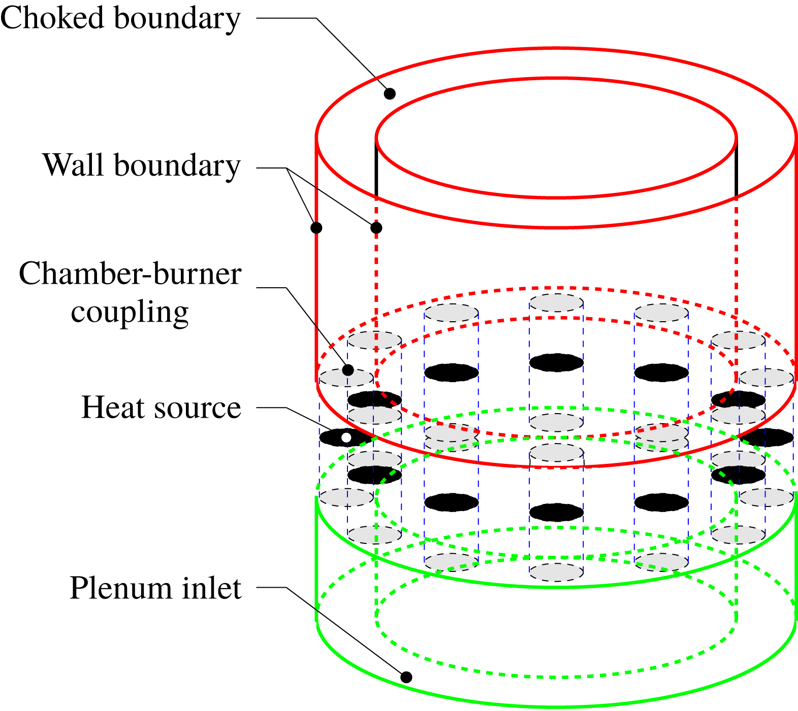
-periodic assemblies of identical units, such as gas turbines (Lieuwen & Yang Reference Lieuwen and Yang2005; Poinsot & Veynante Reference Poinsot and Veynante2005). In order to correctly capture and predict them, it is necessary to devise a model that can account for the dynamics of a single burner as well as the coupling across elements. One-dimensional ducts with a compact heat source are widely used to describe single-burner geometries (Dowling Reference Dowling1995), and here we follow a similar approach. Our model is composed of
 $N$
identical units, assembled in a ring configuration, as shown in figure 1, where the annular geometry is displayed. This model is motivated by the geometrical configuration considered in Laera, Campa & Camporeale (Reference Laera, Campa and Camporeale2017), which consists of
 $N=12$
identical matrix injectors with laminar flow and well-documented flame-describing functions.
Sketch of an
 $N$
-periodic, three-dimensional plenum-burner-chamber configuration consisting of two annular chambers linked by burners.

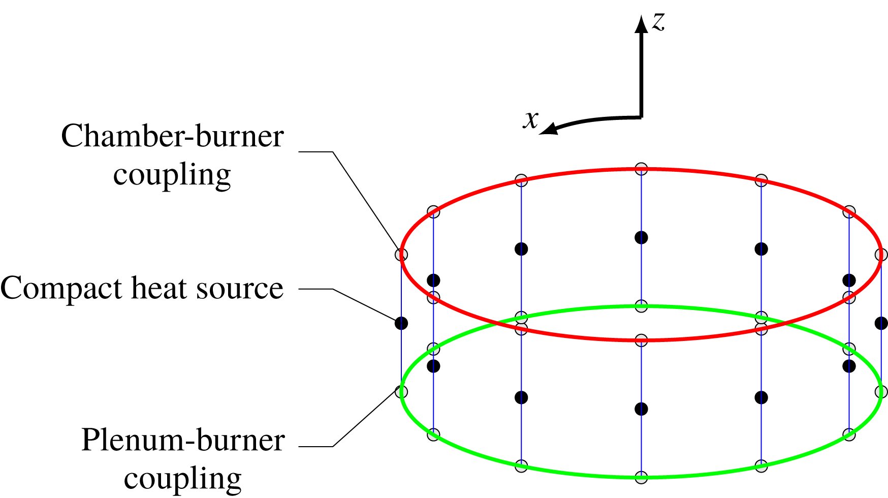
Sketch of an
 $N$
-periodic one-dimensional plenum-burner-chamber configuration consisting of two one-dimensional ring-like chambers coupled together by one-dimensional burners. This simpler model captures the spatial dimensions along which the system’s largest (compared with the compact heater) wavelength acoustic waves manifest themselves inside the combustor.

The
 $N$
-periodic configuration is further simplified by representing the three-dimensional plenum and chamber as one-dimensional annuli and the burners as one-dimensional vertical ducts, each containing a compact heat source, as shown in figure 2. The compact heat source is modelled using a saturation-type nonlinear model that reduces to the linear
 $(n,\unicode[STIX]{x1D70F})$
model in the linear limit (Orchini et al.
Reference Orchini, Rigas and Juniper2016). The top and bottom boundaries of the burner open into the annular chamber and plenum elements of the combustion device. The annulus is modelled only along the periodic azimuthal direction, as illustrated in figure 2. The burner and chamber/plenum elements are coupled together using the jump relation obtained from the conservation of mass at the ends of the burner, where the elements are linked.
2.1 Governing equations
In what follows, we use
 $x$
and
 $z$
as the azimuthal and longitudinal coordinates, respectively, as shown in figure 2. Additionally, the unperturbed base-flow variables, indicated by the subscript
 $_{0}$
, are
 $\unicode[STIX]{x1D70C}_{0}$
,
 $c_{0}$
,
 $p_{0}$
,
 $T_{0}$
and
 $u_{0}\ll c_{0}$
, and they represent density, speed of sound, pressure, temperature and velocity, respectively.
Next, we choose a specific non-dimensionalization such that the
 ${\mathcal{L}}_{2}$
norm of the finite-dimensional state vector, resulting from a discretization of the following equations, corresponds to the non-dimensional acoustic energy of the system. The dimensional variables and coordinates can then be written, using the reference scales for velocity (
 $u_{0,d}$
), pressure
 $(\unicode[STIX]{x1D6FE}p_{0}u_{0,d}/c_{0,d})$
, length (
 $L_{0}$
, the length of the burner) and time (
 $L_{0}/c_{0,d}$
), as follows
 $$\begin{eqnarray}\tilde{u} =u_{0,d}u,\quad \tilde{p}=\unicode[STIX]{x1D6FE}p_{0}\frac{u_{0,d}}{c_{0,d}}p=\unicode[STIX]{x1D6FE}p_{0}Mp,\quad \tilde{x}=L_{0}x,\quad \tilde{t}=(L_{0}/c_{0,d})t,\end{eqnarray}$$
where the quantities with a tilde are dimensional and those without a tilde or subscript
 $_{0}$
are dimensionless. The mean pressure is defined as
 $p_{0}=p_{0,u}=p_{0,d}$
(
 $u_{0,d}/c_{0,d}\ll 1$
) and terms with the
 $_{u}$
or
 $_{d}$
subscripts indicate quantities upstream or downstream of the flame, respectively. In subsequent sections,
 $x_{c}$
,
 $x_{p}$
and
 $z$
coordinates will be used to describe the one-dimensional perimeter of the chamber, plenum and the longitudinal direction along the burners, respectively.
2.1.1 Acoustic equations inside the duct
When a heat source is introduced into the system, the time rate of change of pressure is expressed in terms of the density and entropy as follows,
 $$\begin{eqnarray}\frac{\unicode[STIX]{x2202}\tilde{p}}{\unicode[STIX]{x2202}\tilde{t}}=c_{0}^{2}\frac{\unicode[STIX]{x2202}\tilde{\unicode[STIX]{x1D70C}}}{\unicode[STIX]{x2202}\tilde{t}}+(\unicode[STIX]{x1D6FE}-1)\tilde{\dot{Q}}\,\unicode[STIX]{x1D6FF}(\tilde{z}-\tilde{z}_{f}),\end{eqnarray}$$
where
 $\tilde{\dot{Q}}$
is the heat-release perturbation per unit volume per unit time, given by
 $\tilde{\dot{Q}}=\unicode[STIX]{x1D70C}_{0}T_{0}(\unicode[STIX]{x2202}\tilde{s}/\unicode[STIX]{x2202}\tilde{t})$
(
 $\tilde{s}$
, representing entropy-per-unit-mass perturbations),
 $z_{f}$
is the location of the flame and
 $\unicode[STIX]{x1D6FF}(z)$
represents the Dirac delta distribution along the
 $z$
-axis. Using the definition of
 $c_{0,d}$
, the ideal gas law and equation (2.2) the dimensionless governing equations are given by
 $$\begin{eqnarray}\left\{\begin{array}{@{}l@{}}\displaystyle \frac{\unicode[STIX]{x2202}w}{\unicode[STIX]{x2202}t}+\left(\frac{c_{0}}{c_{0,d}}\right)^{2}\frac{\unicode[STIX]{x2202}p}{\unicode[STIX]{x2202}z}=0,\quad \\ \displaystyle \frac{\unicode[STIX]{x2202}p}{\unicode[STIX]{x2202}t}+\hspace{2.84526pt}\frac{\unicode[STIX]{x2202}w}{\unicode[STIX]{x2202}z}-\unicode[STIX]{x1D708}\frac{\unicode[STIX]{x2202}^{2}p}{\unicode[STIX]{x2202}z^{2}}-\frac{(\unicode[STIX]{x1D6FE}-1)L_{0}}{\unicode[STIX]{x1D6FE}p_{0}w_{0,d}}\tilde{\dot{Q}}\,\unicode[STIX]{x1D6FF}(z-z_{f})=0,\quad \end{array}\right.\end{eqnarray}$$
where,
 $c_{0}$
is a general representation of the speed of sound on either side of the flame,
 $p$
and
 $w$
are the non-dimensional longitudinal pressure and velocity, respectively, within the burners. Equations (2.3) include a term to model dissipative phenomena in the system, with the non-dimensional viscosity denoted by
 $\unicode[STIX]{x1D708}$
. This damping emulates acoustic losses, such as boundary layer losses, within the walls of the modelled annular combustor. A value of the non-dimensional number
 $\unicode[STIX]{x1D708}=0.047$
is chosen to approximate the damping model presented in Sayadi et al. (Reference Sayadi, Le Chenadec, Schmid, Richecoeur and Massot2014) over our frequency range of interest. The heat-release model is then invoked to provide the following nonlinear representation of the heat-release perturbations per unit volume per unit time, in non-dimensional form, as
 $$\begin{eqnarray}\frac{(\unicode[STIX]{x1D6FE}-1)L_{0}}{\unicode[STIX]{x1D6FE}p_{0}w_{0,d}}\tilde{\dot{Q}}=nf(w_{f,\unicode[STIX]{x1D70F}}),\end{eqnarray}$$
where
 $f(w_{f,\unicode[STIX]{x1D70F}})=\unicode[STIX]{x1D6FC}_{1}w_{f,\unicode[STIX]{x1D70F}}+\unicode[STIX]{x1D6FC}_{2}w_{f,\unicode[STIX]{x1D70F}}^{2}+\unicode[STIX]{x1D6FC}_{3}w_{f,\unicode[STIX]{x1D70F}}^{3}+\unicode[STIX]{x1D6FC}_{4}w_{f,\unicode[STIX]{x1D70F}}^{4}+\unicode[STIX]{x1D6FC}_{5}w_{f,\unicode[STIX]{x1D70F}}^{5}$
and
 $n$
stands for the non-dimensional strength of the flame. The velocity
 $w_{f,\unicode[STIX]{x1D70F}}$
is commonly taken to be the velocity value on the cold side of the heat source with a time delayed (
 $\unicode[STIX]{x1D70F}$
) flame response; the coefficients
 $\unicode[STIX]{x1D6FC}_{i},\;i=1,\ldots ,5$
, depend on the choice of the flame model. In this study we use the values
 $$\begin{eqnarray}\unicode[STIX]{x1D6FC}_{1}=1,\quad \unicode[STIX]{x1D6FC}_{2}=-0.33,\quad \unicode[STIX]{x1D6FC}_{3}=0.0028,\quad \unicode[STIX]{x1D6FC}_{4}=0.1736,\quad \unicode[STIX]{x1D6FC}_{5}=-0.0636,\end{eqnarray}$$
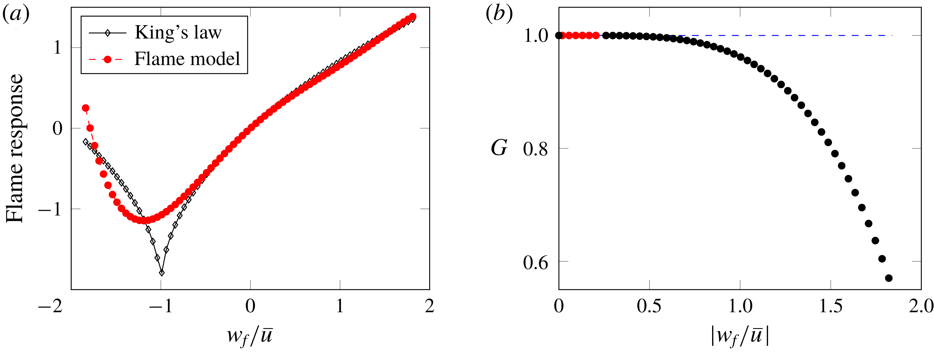
in order to approximate the saturation-type nonlinearity demonstrated by King’s law. Section 4.2.5 discusses this model and the
 $\unicode[STIX]{x1D6FC}_{i}$
in more detail. This, however, does not pose any restrictions on the subsequent analysis, as any saturation-type functional relation can be substituted for King’s law without loss of generality.
2.1.2 Coupling the chamber and the plenum to the duct
While (2.3) are used to represent the flame dynamics and the propagation of the longitudinal acoustic perturbations within the burner sub-units, they have yet to be linked in the azimuthal direction to the annular chamber and plenum. This is realized by coupling the modified wave equation (2.3) solved over the one-dimensional burner elements parallel to the axis of symmetry, with the dissipative wave equation (equations (2.3) without the flame) solved over the one-dimensional azimuthal direction perpendicular to the axis of symmetry, whilst ensuring the conservation of mass at the ends of the burner. The integral terms in (2.6) appear as a consequence of the surface integral computed to ensure the conservation of mass at the ends of the burner (refer to appendix A for details). This form of coupling was inspired by work presented in Bauerheim et al. (Reference Bauerheim, Parmentier, Salas, Nicoud and Poinsot2014). The final set of equations that results from this azimuthal coupling, along the coordinates of
 $x_{c}$
and
 $x_{p}$
that represent the perimeter of the chamber and plenum, respectively, is expressed as
 $$\begin{eqnarray}\left\{\begin{array}{@{}l@{}}\displaystyle \frac{\unicode[STIX]{x2202}u}{\unicode[STIX]{x2202}t}+\left(\frac{c_{0}}{c_{0,d}}\right)^{2}\frac{\unicode[STIX]{x2202}p}{\unicode[STIX]{x2202}x}=0,\quad \\ \displaystyle \frac{\unicode[STIX]{x2202}p}{\unicode[STIX]{x2202}t}+\frac{\unicode[STIX]{x2202}u}{\unicode[STIX]{x2202}x}-\unicode[STIX]{x1D708}\frac{\unicode[STIX]{x2202}^{2}p}{\unicode[STIX]{x2202}x^{2}}=0,\quad \\ \displaystyle \frac{\unicode[STIX]{x2202}p}{\unicode[STIX]{x2202}t}+\left(\frac{\unicode[STIX]{x2202}u}{\unicode[STIX]{x2202}x_{c}}-\frac{wS_{b}}{\displaystyle \int S_{c}\,\text{d}x_{c}}\right)-\unicode[STIX]{x1D708}\left(\frac{\unicode[STIX]{x2202}^{2}p}{\unicode[STIX]{x2202}x_{c}^{2}}-\frac{S_{i}(\unicode[STIX]{x2202}p/\unicode[STIX]{x2202}z)|_{z=1}}{\displaystyle \int S_{c}\,\text{d}x_{c}}\right)=0\quad \text{when}~x_{c}=x_{b,c},\quad \\ \displaystyle \frac{\unicode[STIX]{x2202}p}{\unicode[STIX]{x2202}t}+\left(\frac{\unicode[STIX]{x2202}u}{\unicode[STIX]{x2202}x_{p}}+\frac{wS_{b}}{\displaystyle \int S_{p}\,\text{d}x_{p}}\right)-\unicode[STIX]{x1D708}\left(\frac{\unicode[STIX]{x2202}^{2}p}{\unicode[STIX]{x2202}x_{p}^{2}}+\frac{S_{i}(\unicode[STIX]{x2202}p/\unicode[STIX]{x2202}z)|_{z=0}}{\displaystyle \int S_{p}\,\text{d}x_{p}}\right)=0\quad \text{when}~x_{p}=x_{b,p},\quad \end{array}\right.\end{eqnarray}$$
in the chamber. Here,
 $(p,u)$
denote the pressure and axial velocity along the perimeter of the chamber (or plenum), respectively. The coordinates
 $x_{b,c}$
(or
 $x_{b,p}$
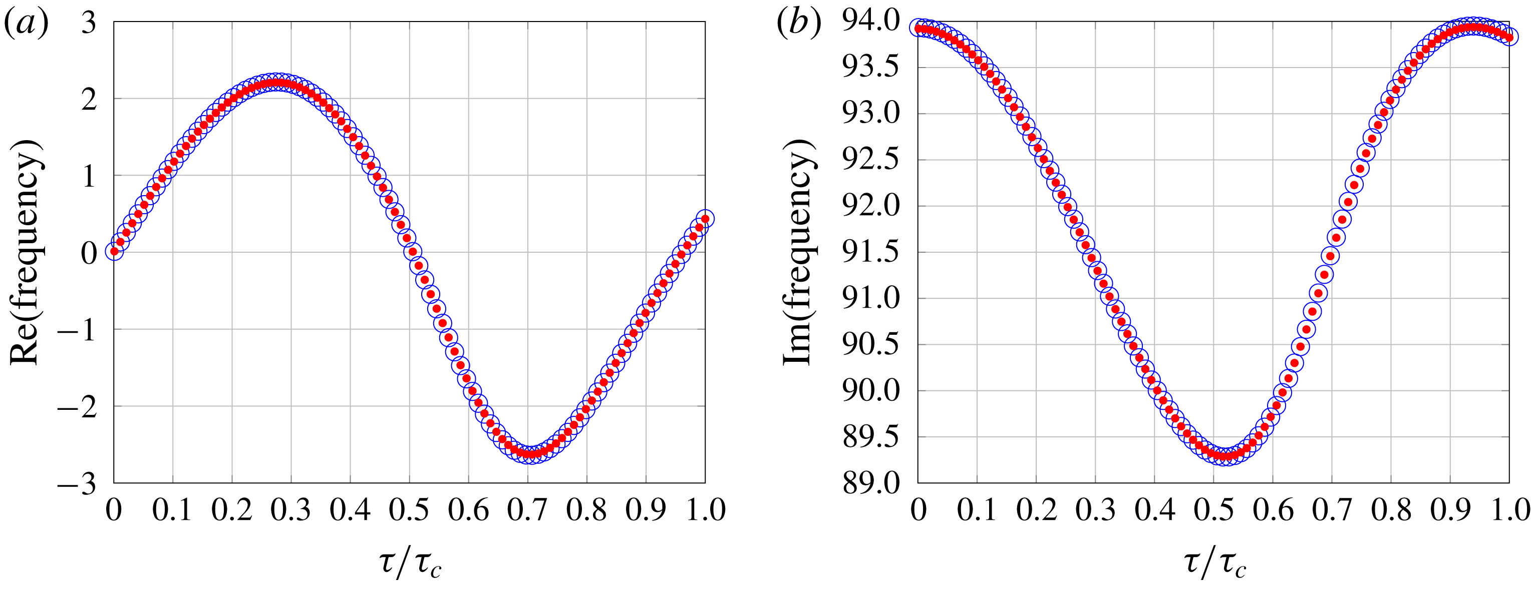
) represent the location where a burner is coupled to the chamber (or plenum). This model was discretized as per § 3 and verified, in the linear regime, against the network model proposed in Bauerheim et al. (Reference Bauerheim, Parmentier, Salas, Nicoud and Poinsot2014). The verification is demonstrated in figure 3 where the real and imaginary part of the eigenfrequency corresponding to the first weakly coupled chamber mode (WCC1; Bauerheim et al.
Reference Bauerheim, Parmentier, Salas, Nicoud and Poinsot2014) for an annular combustor with four burner elements, both from the network model and the discrete state-space model (with an appropriately modified heat source), are successfully matched.
Real (a) and imaginary (b) parts of the eigenfrequency corresponding to the first weakly coupled chamber mode. Red and blue circles represent the network model and discrete state-space model results, respectively.
 $\unicode[STIX]{x1D70F}/\unicode[STIX]{x1D70F}_{c}$
represents the non-dimensional time delay associated with the flame (Bauerheim et al.
Reference Bauerheim, Parmentier, Salas, Nicoud and Poinsot2014).

2.2 Global dynamics from single-unit analysis
The governing equations for the plenum burner and chamber configurations have to be formulated for an assembly of
 $N$
identical subunits. This formulation reveals a distinct structure of the governing system matrix: a block-circulant layout, where each identical block on the diagonal describes the motion in each unit, while the off-diagonal blocks account for the interaction with other units. In the analysis of the global system of
 $N$
units, this block-circulant structure can be exploited, and all computations can be performed on a single unit without forgoing the inter-unit and trans-unit dynamics. The mathematical transformation from the global system of equations to a single-unit formulation uses a roots-of-unity concept, which is equivalent to a Bloch-wave formalism; details can be found in Schmid et al. (Reference Schmid, Fosas de Pando and Peake2017).
Any desired quantity of the full system, either modal or non-modal, can then be formulated on a single-unit system and computed while varying the root of unity. Here, the root-of-unity index (
 $j$
) refers to a form of boundary condition specifying the phase difference (
 $2\unicode[STIX]{x03C0}j/N$
) across a single sector, of a solution, in the azimuthal direction. In addition, the mutual influence of distinct units as well as the trans-unit dynamics can be described and quantified by considering only a sequence of single-unit systems. As a consequence, the computational cost (e.g. for a modal analysis) is reduced from
 $O(N^{3}h^{3})$
for the full global analysis to
 $O(Nh^{3})$
where
 $h$
represents the number of degrees of freedom in a single unit; a savings factor of
 $N^{2}$
can be realized for our case of
 $N=12$
units, which is a savings of two orders of magnitude.
3 Numerical framework
This section describes the proposed discrete state-space model, including the numerical treatment of the spatial operators, the coupling between the plenum, burner and chamber components of the combustor and the time delay inherent to the nonlinear flame model present in the set of (2.3) and (2.6).
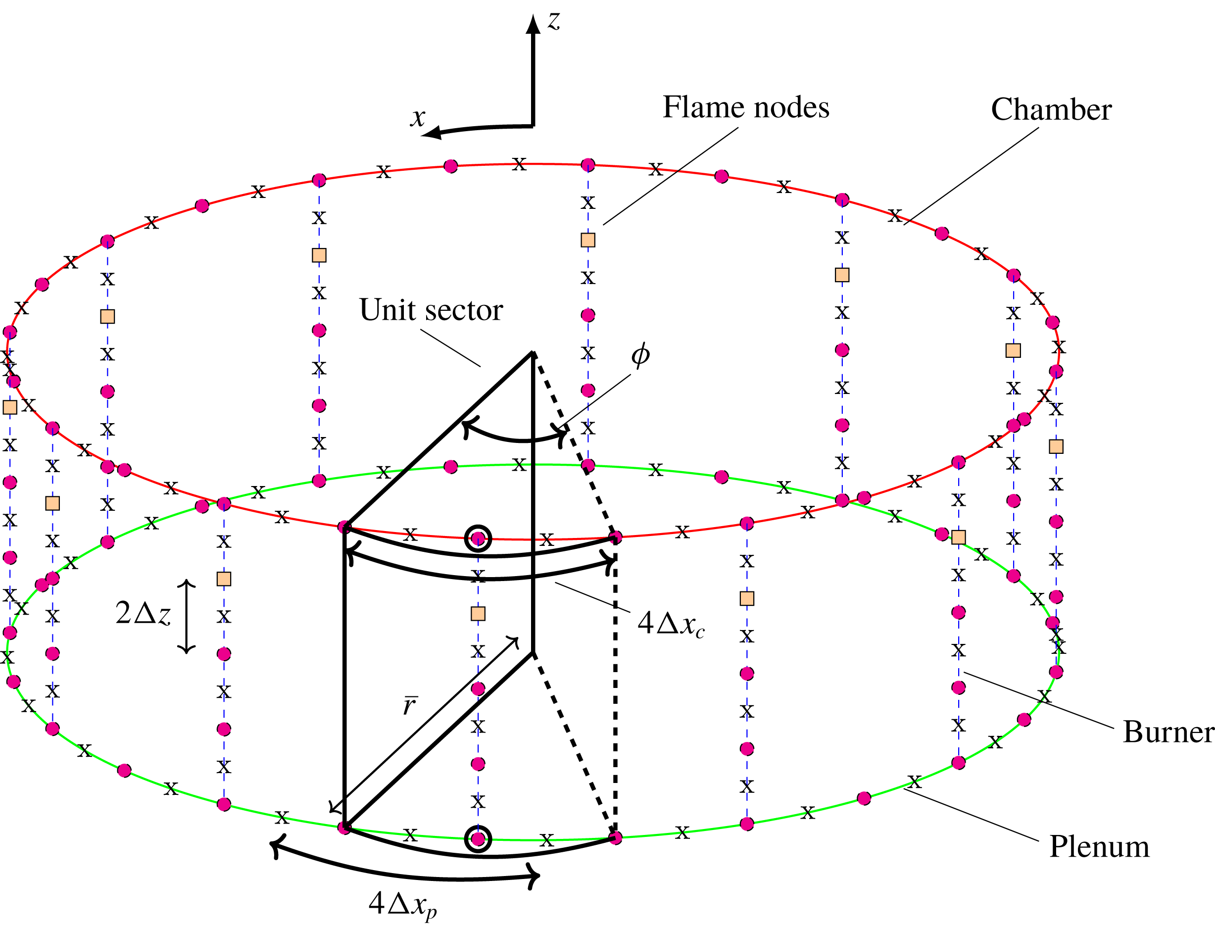
Staggered grid formation of pressures (circles) and velocities (x) within the one-dimensional plenum-burner-chamber geometry. The angle subtended and the mean radius of the unit sector are labelled as
 $\unicode[STIX]{x1D719}=2\unicode[STIX]{x03C0}/N$
and
 $\bar{r}$
, respectively. The pressure discretization points at which the burner is coupled to the chamber and plenum are highlighted. The pressure and velocity discretization points within the unit sector (except those on the dashed lines) constitute that sector’s state variables.

3.1 Discretized governing equations: chamber/plenum
A staggered arrangement of the variables on a one-dimensional axisymmetric structured mesh (see figure 4) is used to discretize the chamber/plenum geometry. The azimuthal boundary conditions are specified according to the roots-of-unity formalism for single-sector (unit-sector) computations. The spatial derivatives across the chamber are represented using a second-order centred difference approximation.
In what follows, subscript
 $\text{}_{\unicode[STIX]{x1D709}}$
represents either chamber (
 $\text{}_{c}$
) or plenum (
 $\text{}_{p}$
) specific quantities. The resulting unit-sector state vector corresponding to the chamber/plenum, containing
 $M_{\unicode[STIX]{x1D709}}$
pressure discretization points, and an equal number of velocity discretization points, is given by
 $$\begin{eqnarray}\boldsymbol{x}_{\unicode[STIX]{x1D709}}=[p_{\unicode[STIX]{x1D709}}^{1},u_{\unicode[STIX]{x1D709}}^{1},p_{\unicode[STIX]{x1D709}}^{2},u_{\unicode[STIX]{x1D709}}^{2},\ldots ,p_{\unicode[STIX]{x1D709}}^{M_{\unicode[STIX]{x1D709}}},u_{\unicode[STIX]{x1D709}}^{M_{\unicode[STIX]{x1D709}}}]^{\text{T}}.\end{eqnarray}$$
Discretization of the governing equations (2.3), without the flame, takes the following form
 $$\begin{eqnarray}\displaystyle \frac{\text{d}u_{\unicode[STIX]{x1D709}}^{i}}{\text{d}t} & = & \displaystyle -\left(\frac{c_{0}}{c_{0,d}}\right)^{2}\left(\frac{p_{\unicode[STIX]{x1D709}}^{i+1}-p_{\unicode[STIX]{x1D709}}^{i}}{2\unicode[STIX]{x0394}x_{\unicode[STIX]{x1D709}}}\right),\end{eqnarray}$$
 $$\begin{eqnarray}\displaystyle \frac{\text{d}p_{\unicode[STIX]{x1D709}}^{i}}{\text{d}t} & = & \displaystyle -\left(\frac{u_{\unicode[STIX]{x1D709}}^{i}-u_{\unicode[STIX]{x1D709}}^{i-1}}{2\unicode[STIX]{x0394}x_{\unicode[STIX]{x1D709}}}\right)+\unicode[STIX]{x1D708}\left(\frac{p_{\unicode[STIX]{x1D709}}^{i+1}-2p_{\unicode[STIX]{x1D709}}^{i}+p_{\unicode[STIX]{x1D709}}^{i-1}}{4\unicode[STIX]{x0394}x_{\unicode[STIX]{x1D709}}^{2}}\right).\end{eqnarray}$$
 $i\in \{1,M_{\unicode[STIX]{x1D709}}\}$
, else the roots-of-unity method imposes a boundary condition of the form
 $u_{\unicode[STIX]{x1D709}}^{0}=u_{\unicode[STIX]{x1D709}}^{M_{\unicode[STIX]{x1D709}}}/\unicode[STIX]{x1D70C}_{j}$
and
 $p_{\unicode[STIX]{x1D709}}^{0}=p_{\unicode[STIX]{x1D709}}^{M_{\unicode[STIX]{x1D709}}}/\unicode[STIX]{x1D70C}_{j}$
when
 $i=1$
, and
 $p_{\unicode[STIX]{x1D709}}^{M_{\unicode[STIX]{x1D709}}+1}=p_{\unicode[STIX]{x1D709}}^{1}\unicode[STIX]{x1D70C}_{j}$
when
 $i=M_{\unicode[STIX]{x1D709}}$
, where
 $\unicode[STIX]{x1D70C}_{j}=\exp (\text{i}2\unicode[STIX]{x03C0}\mathit{j}/\mathit{N})$
.
A discrete dynamical-system representation of the stand-alone chamber/plenum equations (2.6) can then be represented by
 $$\begin{eqnarray}\displaystyle \dot{\boldsymbol{x}}_{\unicode[STIX]{x1D709}} & = & \displaystyle \{\unicode[STIX]{x1D63C}_{\unicode[STIX]{x1D709}}^{\prime }(j)-\unicode[STIX]{x1D708}(S_{b}/(S_{\unicode[STIX]{x1D709}}\,4\unicode[STIX]{x0394}x_{\unicode[STIX]{x1D709}}\unicode[STIX]{x0394}z))\hat{\boldsymbol{e}}_{i_{\unicode[STIX]{x1D709}}}\otimes \hat{\boldsymbol{e}}_{i_{\unicode[STIX]{x1D709}}}^{\text{T}}\}\boldsymbol{x}_{\unicode[STIX]{x1D709}}+\unicode[STIX]{x1D63C}_{\unicode[STIX]{x1D709}b}\,\boldsymbol{x}_{b},\end{eqnarray}$$
 $$\begin{eqnarray}\displaystyle & = & \displaystyle \unicode[STIX]{x1D63C}_{\unicode[STIX]{x1D709}}(j)\boldsymbol{x}_{\unicode[STIX]{x1D709}}+\unicode[STIX]{x1D63C}_{\unicode[STIX]{x1D709}b}\,\boldsymbol{x}_{b},\end{eqnarray}$$
 $\unicode[STIX]{x1D63C}_{\unicode[STIX]{x1D709}}^{\prime }$
is constructed using equation set (3.2), matrix
 $\unicode[STIX]{x1D63C}_{\unicode[STIX]{x1D709}b}$
represents the additional terms, mentioned in (2.6), that describe the influence of the burner on the shared pressure discretization points within each cavity, and
 $i_{\unicode[STIX]{x1D709}}$
is the index of the coupled pressure node (highlighted in figure 4 with dark circles), within each cavity and at the ends of a burner, in vector
 $\boldsymbol{x}_{\unicode[STIX]{x1D709}}$
.
3.2 Discretized governing equations: burner
A staggered arrangement of the variables is also used to discretize the one-dimensional burner geometry (see figure 4). The boundary conditions at the first and last pressure discretization points of the burner, located at
 $z=0$
and
 $z=1$
accordingly, are inferred by the coupling with the plenum and the chamber. The numerical framework of Sayadi et al. (Reference Sayadi, Le Chenadec, Schmid, Richecoeur and Massot2014) is adopted here, where the spatial derivatives along the burner are represented using a second-order centred difference scheme. A ghost fluid treatment (Fedkiw et al.
Reference Fedkiw, Aslam, Merriman and Osher1999) for the velocity discontinuity across the heat source is employed to retain the compact character of the acoustic source, formally reducing the order of accuracy to first order in the vicinity of the singularity. In this formalism, the heat source coincides with a pressure node. The spatial discretization is completed by the approximation of the damping, as described in § 2.1, and is presented in the following for a unit sector.
The state vector corresponding to the burner, containing
 $M_{b}$
pressure discretization points and
 $M_{b}+1$
velocity discretization points, is given by
 $$\begin{eqnarray}\boldsymbol{x}_{b}=[w_{b}^{1},p_{b}^{1},w_{b}^{2},p_{b}^{2},\ldots ,p_{b}^{M_{b}},w_{b}^{M_{b}+1}]^{\text{T}}.\end{eqnarray}$$
Discretization of the governing equations (2.3) without the flame, in case of the burner, is the same as for (3.2), once we account for the structure of
 $\boldsymbol{x}_{b}$
. The pressure discretization points at the ends of the burner are shared with the plenum and chamber units. The temporal evolution of pressure at these shared discretization points is governed by their respective mass flux and viscous dissipation, influenced both by the burner and annular chamber/plenum. The discrete equation governing the rate of change of pressure at these points is discussed in § 3.3.
A discrete dynamical-system representation of the stand-alone burner equations (2.3) can then be represented by
 $$\begin{eqnarray}\dot{\boldsymbol{x}}_{b}=\unicode[STIX]{x1D63C}_{b}\,\boldsymbol{x}_{b}+\unicode[STIX]{x1D63C}_{bc}\,\boldsymbol{x}_{c}+\unicode[STIX]{x1D63C}_{bp}\,\boldsymbol{x}_{p}+n\,f(w_{b}^{i_{f}}(t-\unicode[STIX]{x1D70F}))\,\hat{\boldsymbol{e}}_{(i_{f}-1)},\end{eqnarray}$$
where,
 $\hat{\boldsymbol{e}}_{i}$
is the unit vector with a unit entry at the
 $i$
th index,
 $i_{f}\,\unicode[STIX]{x0394}z=z_{f}$
(
 $\unicode[STIX]{x0394}z$
, as shown in figure 4, is half the distance between two pressure discretization points within each burner), matrix
 $\unicode[STIX]{x1D63C}_{b}$
is constructed using the appropriately modified system of (2.3) and matrices
 $\unicode[STIX]{x1D63C}_{bc}$
and
 $\unicode[STIX]{x1D63C}_{bp}$
represent the burner-chamber and burner-plenum coupling, respectively. Implementation of the delayed term
 $w_{b}^{i_{b}}(t-\unicode[STIX]{x1D70F})$
is explained in § 3.4.
3.3 Discretized governing equations: combined plenum-burner-chamber equations
The structure of the nonlinear dynamical system, representing equations (2.3) and (2.6) within a unit sector (shown in figure 4), is now given by
 $$\begin{eqnarray}\dot{\boldsymbol{x}}_{us}=\left[\begin{array}{@{}ccc@{}}\unicode[STIX]{x1D63C}_{c}(j) & \unicode[STIX]{x1D63C}_{cb} & 0\\ \unicode[STIX]{x1D63C}_{bc} & \unicode[STIX]{x1D63C}_{b} & \unicode[STIX]{x1D63C}_{bp}\\ 0 & \unicode[STIX]{x1D63C}_{pb} & \unicode[STIX]{x1D63C}_{p}(j)\end{array}\right]\boldsymbol{x}_{us}+\left[\begin{array}{@{}c@{}}0\\ n\,f(w_{b}^{i_{f}}(t-\unicode[STIX]{x1D70F}))\hat{\boldsymbol{e}}_{i_{f}}\\ 0\end{array}\right],\end{eqnarray}$$
where,
 $\boldsymbol{x}_{us}=[\boldsymbol{x}_{c}^{\text{T}},\boldsymbol{x}_{b}^{\text{T}},\boldsymbol{x}_{p}^{\text{T}}]^{\text{T}}$
, matrices of the form
 $\unicode[STIX]{x1D63C}_{b\unicode[STIX]{x1D709}}$
and
 $\unicode[STIX]{x1D63C}_{\unicode[STIX]{x1D709}b}$
are given by
 $$\begin{eqnarray}\displaystyle \unicode[STIX]{x1D63C}_{bc} & = & \displaystyle -(c_{0}^{2}/(c_{0,d}^{2}\,2\unicode[STIX]{x0394}z))\hat{\boldsymbol{e}}_{2M_{b}+1}\otimes \hat{\boldsymbol{e}}_{i_{c}}^{\text{T}},\end{eqnarray}$$
 $$\begin{eqnarray}\displaystyle \unicode[STIX]{x1D63C}_{bp} & = & \displaystyle (c_{0}^{2}/(c_{0,d}^{2}\,2\unicode[STIX]{x0394}z))\hat{\boldsymbol{e}}_{1}\otimes \hat{\boldsymbol{e}}_{i_{p}}^{\text{T}},\end{eqnarray}$$
 $$\begin{eqnarray}\displaystyle \unicode[STIX]{x1D63C}_{cb} & = & \displaystyle (S_{b}/(S_{c}\,2\unicode[STIX]{x0394}x_{c}))\hat{\boldsymbol{e}}_{i_{c}}\otimes \hat{\boldsymbol{e}}_{2M_{b}+1}^{\text{T}}+\unicode[STIX]{x1D708}\{(S_{b}/(S_{c}\,4\unicode[STIX]{x0394}x_{c}\unicode[STIX]{x0394}z))\hat{\boldsymbol{e}}_{i_{c}}\otimes \hat{\boldsymbol{e}}_{2M_{b}}^{\text{T}}\},\end{eqnarray}$$
 $$\begin{eqnarray}\displaystyle \unicode[STIX]{x1D63C}_{pb} & = & \displaystyle -(S_{b}/(S_{p}\,2\unicode[STIX]{x0394}x_{p}))\hat{\boldsymbol{e}}_{i_{p}}\otimes \hat{\boldsymbol{e}}_{1}^{\text{T}}+\unicode[STIX]{x1D708}\{(S_{b}/(S_{p}\,4\unicode[STIX]{x0394}x_{p}\unicode[STIX]{x0394}z))\hat{\boldsymbol{e}}_{i_{p}}\otimes \hat{\boldsymbol{e}}_{2}^{\text{T}}\}.\end{eqnarray}$$
3.4 Spectral and bifurcation analysis
The discretization and subsequent linearization of (2.3) and (2.6) yield a set of linear delay-differential equations (DDEs). The stability properties of such systems can be analysed using a technique proposed by Jarlebring (Reference Jarlebring2008), which recasts the original DDE as a partial differential equation by introducing an additional independent variable in the form of a space-like memory dimension.
The analysis is performed on the discretized system of equations (3.6), with the linearized version of the source term from the flame model given in (2.4). The parameters of interest in the ensuing spectral and bifurcation analysis are the non-dimensional flame strength
 $n$
, its location
 $z_{f}$
and the delay time
 $\unicode[STIX]{x1D70F}$
. The roots-of-unity formalism yields
 $N$
decoupled and linear semi-discrete delay differential equations for each
 $j\in \{0,\ldots ,N-1\}$
, cast in matrix form according to
 $$\begin{eqnarray}\dot{\boldsymbol{x}}_{us}=\underbrace{\left[\begin{array}{@{}ccc@{}}\unicode[STIX]{x1D63C}_{c}(j) & \unicode[STIX]{x1D63C}_{cb} & 0\\ \unicode[STIX]{x1D63C}_{bc} & \unicode[STIX]{x1D63C}_{b} & \unicode[STIX]{x1D63C}_{bp}\\ 0 & \unicode[STIX]{x1D63C}_{pb} & \unicode[STIX]{x1D63C}_{p}(j)\end{array}\right]}_{\unicode[STIX]{x1D63C}_{0}(j)}\boldsymbol{x}_{us}+\underbrace{\left[\begin{array}{@{}ccc@{}}0 & 0 & 0\\ 0 & n\unicode[STIX]{x1D63C}_{b}\hspace{2.84526pt}\hat{\boldsymbol{e}}_{(i_{f}-1)}^{\text{T}} & 0\\ 0 & 0 & 0\end{array}\right]}_{\unicode[STIX]{x1D63C}_{1}}\boldsymbol{x}_{us}(t-\unicode[STIX]{x1D70F}).\end{eqnarray}$$
The matrix
 $\unicode[STIX]{x1D63C}_{0}(j)$
contains differentiation and damping operators together with the
 $j$
th root-of-unity azimuthal boundary condition, and
 $\unicode[STIX]{x1D63C}_{1}$
includes the linearized heat source. The eigenvectors and eigenvalues of this matrix satisfy the following relation (Jarlebring Reference Jarlebring2008)
 $$\begin{eqnarray}(\unicode[STIX]{x1D63C}_{0}(j)+\unicode[STIX]{x1D63C}_{1}e^{-\unicode[STIX]{x1D70F}\unicode[STIX]{x1D706}})\boldsymbol{v}=\unicode[STIX]{x1D706}\boldsymbol{v},\end{eqnarray}$$
where
 $\boldsymbol{v}$
represents an eigenvector and
 $\unicode[STIX]{x1D706}$
the associated eigenvalue. Equation (3.9) constitutes a nonlinear eigenvalue problem that can be solved numerically using the partial differential equation (PDE) method (Jarlebring Reference Jarlebring2008), which recasts the above equation into the following form, linear in
 $\boldsymbol{v}^{\prime }$
,
 $$\begin{eqnarray}\unicode[STIX]{x1D63C}_{\unicode[STIX]{x1D70F}}(j)\boldsymbol{v}^{\prime }=\left[\begin{array}{@{}c@{}}\unicode[STIX]{x1D63F}_{K-1}\otimes \unicode[STIX]{x1D644}_{k}\\ \unicode[STIX]{x1D63C}_{1}~0~\cdots ~0~\unicode[STIX]{x1D63C}_{0}(j)\end{array}\right]\boldsymbol{v}^{\prime }=\unicode[STIX]{x1D706}^{\prime }\boldsymbol{v}^{\prime },\end{eqnarray}$$
where
 $\unicode[STIX]{x1D63F}_{K-1}$
is the
 $K-1$
dimensional Chebyshev differentiation matrix (see Trefethen Reference Trefethen2000). The above formulation encapsulates the discretization of the space-like memory (
 $[t-\unicode[STIX]{x1D70F},t]$
) dimension, and
 $\unicode[STIX]{x1D644}_{k}$
denotes the identity matrix with the same dimensions as
 $\unicode[STIX]{x1D63C}_{1}$
. Equation (3.10) is now a linear eigenvalue problem, but of larger dimension, which can be solved using standard eigen-decomposition techniques. It is worth mentioning that the vector
 $\boldsymbol{v}^{\prime }$
contains an approximation of the eigenvector
 $\boldsymbol{v}$
at
 $K$
Chebyshev collocation points in time within the duration
 $[t-\unicode[STIX]{x1D70F},t]$
. Thus, in order to obtain an approximation for
 $\boldsymbol{v}(t)$
we must choose the last
 $k$
entries within the vector
 $\boldsymbol{v}^{\prime }$
of size
 $K\times k$
. The numerical techniques reported in Jarlebring (Reference Jarlebring2008) are available in the software package DDE-BIFTOOL (Engelborghs, Luzyanina & Samaey Reference Engelborghs, Luzyanina and Samaey2000), which is employed in this article to obtain neutral curves, corresponding to different roots-of-unity values, against the parameters
 $n$
and
 $\unicode[STIX]{x1D70F}$
, for selection of geometry, coupling parameters and flame locations.
4 Results and discussion
In this section, the discrete model will be applied to the plenum-burner-chamber (PBC) configuration described in § 2, focusing on the influence of model parameters such as flame strength and delay on the linear stability of the PBC system. This modal analysis will establish the bounds in parameter space that delineate asymptotic stability from unstable long-time behaviour. Crossing these boundaries into the unstable regime calls into action nonlinear effects that, fuelled by the instability, will yield saturated states at finite amplitudes. A weakly nonlinear analysis, taking into account a selected group of nonlinearities via an asymptotic, multi-scale expansion, will give insight into saturated states and will track linear instabilities to their finite-amplitude states. The nature of this continuation classifies the associated bifurcation as super- or sub-critical, and in the case of subcritical bifurcations motivates a non-modal analysis to establish the existence (and nature) of transient energy growth to reach finite-amplitude states even under subcritical conditions. In other words, the linear and non-modal analyses provide insight into the short-term response to broadband environmental noise or to a specific excitation by components upstream or downstream of the combustion unit, whilst the manner in which such disturbances can pulse the system from a stable base flow to sustained oscillations is quantified by a weakly nonlinear asymptotic expansion of the system’s behaviour. This uniformly valid asymptotic expansion introduces multiple time scales to formally separate the fast and the slow dynamics. The fast time scale and the bifurcation point can be obtained from a linear stability analysis, on the other hand, the nonlinear evolution of the system close to this critical point can be described by a complex amplitude that is a function of the slow time scales. This amplitude evolution equation is given in the form of an ordinary differential equation, appearing as a Stuart–Landau equation, for every linearly unstable mode. Solving the latter equation is noticeably faster than time marching the full nonlinear system and provides insight into the nonlinear interactions between the modes.
The twelve-burner geometrical configuration of the PBC system that we investigate has a heat source within each burner element (of length
 $L_{0}=0.0508$
m) at a distance
 $z_{f}=0.88L_{0}$
from the boundary it shares with the plenum. The location
 $z_{f}$
is chosen so that it does not coincide with any pressure nodes within the system (Bauerheim et al.
Reference Bauerheim, Parmentier, Salas, Nicoud and Poinsot2014). The burners themselves are coupled, in an
 $N$
-periodic fashion, along the perimeter of the chamber and plenum of the PBC system. The inner radius, outer radius and height of the chamber are taken to be
 $0.24$
m,
 $0.197$
m and
 $0.6$
m, respectively. Similarly, the inner radius, outer radius and height of the plenum are taken to be
 $0.24425$
m,
 $0.19275$
m and
 $0.1$
m, respectively. These dimensions are similar to the annular test case considered in Laera et al. (Reference Laera, Campa and Camporeale2017), but were modified by reducing the diameter and height of the plenum as well as increasing the height of the chamber to cause the first Hopf bifurcation to appear for a degenerate weakly coupled chamber mode (Bauerheim et al.
Reference Bauerheim, Parmentier, Salas, Nicoud and Poinsot2014). This specific coupling between the components of the PBC configuration also ensures that the mode associated with the system’s Hopf bifurcation is the lowest-frequency, globally periodic (system-scale), (
 $j=1$
) azimuthal eigenmode (figure 5
b) belonging to an eigenspace of dimension two; this particular degeneracy is critical in describing the nonlinear behaviour of the system.
4.1 Modal analysis
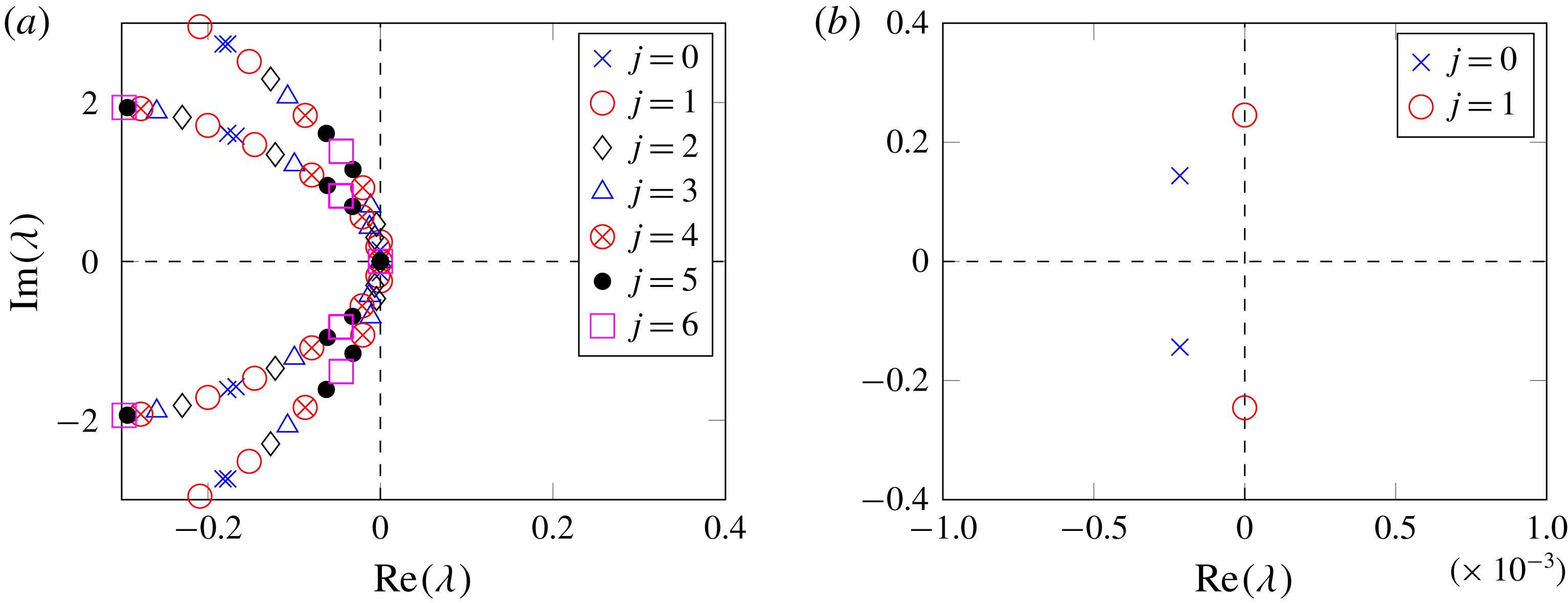
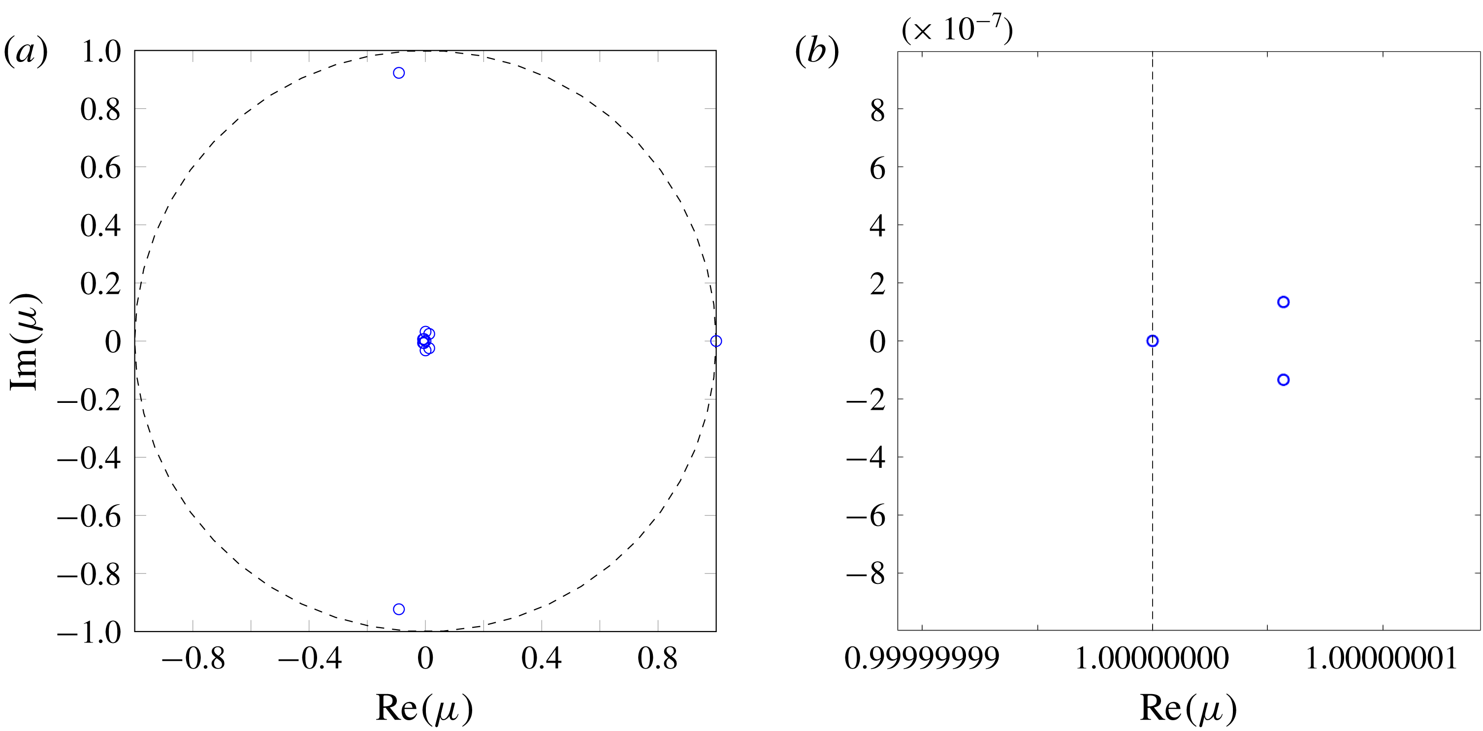
We start by assessing the modal stability of thermo-acoustic waves in the PBC system based on a spectral analysis. Modal shapes and neutral curves of the configuration are also computed in order to shed more light on the systems linear stability. The spectrum, for non-dimensional time delay
 $\unicode[STIX]{x1D70F}=3.85$
and flame strength
 $n=0.2425$
, is displayed in figures 5(a) and 5(b). These parameters mark the onset of instabilities in the system, when the neutral curve corresponding to the root of unity
 $j=1$
shows a transition in linear stability and alters the dynamical behaviour of the
 $N$
-periodic system. Since, in this example, the
 $N$
-periodic system consists of
 $12$
units,
 $12$
solutions of the roots-of-unity algorithm exist. However, roots for
 $j$
and
 $N-j$
(where
 $j\in \{1,\ldots ,N-1\}$
) yield the same eigenspectrum, stemming from degeneracy of dimension two.
It is worth mentioning two exceptions to this rule: the first, when
 $j$
is a multiple of
 $N/2$
for even
 $N,$
and the second, when
 $j$
is a multiple of
 $N$
for odd
 $N.$
Returning to the system’s inherent degeneracy, we observe that while this is responsible for the rich nonlinear thermo-acoustic behaviour in annular combustion chambers (Ghirardo et al.
Reference Ghirardo, Juniper and Moeck2016), it does not affect the modal behaviour (stability) of the system, and, hence, in all spectral and bifurcation plots, only a subset of the roots of unity with
 $j=0,1,\ldots ,6$
are considered. However, this degeneracy strongly affects the system’s sensitivity to small-amplitude disturbances: a point that will be addressed in the following section describing the weakly nonlinear analysis. The spectrum displayed in figure 5(a), reveals two distinct branches in the system’s eigenspectrum. These branches are a consequence of the mismatch in the speed of sound intrinsic to the plenum (unburnt) and chamber (burnt) units of the model. In addition, the dynamical system under consideration is finite-dimensional which, together with the existing delay, results in a large spectrum, representing both the coupled and the uncoupled modes of the PBC configuration.
Eigenspectra of the PBC configuration for (a)
 $n=0.2425$
and
 $\unicode[STIX]{x1D70F}=3.85,$
and (b) close-up of the eigenspectrum in (a).

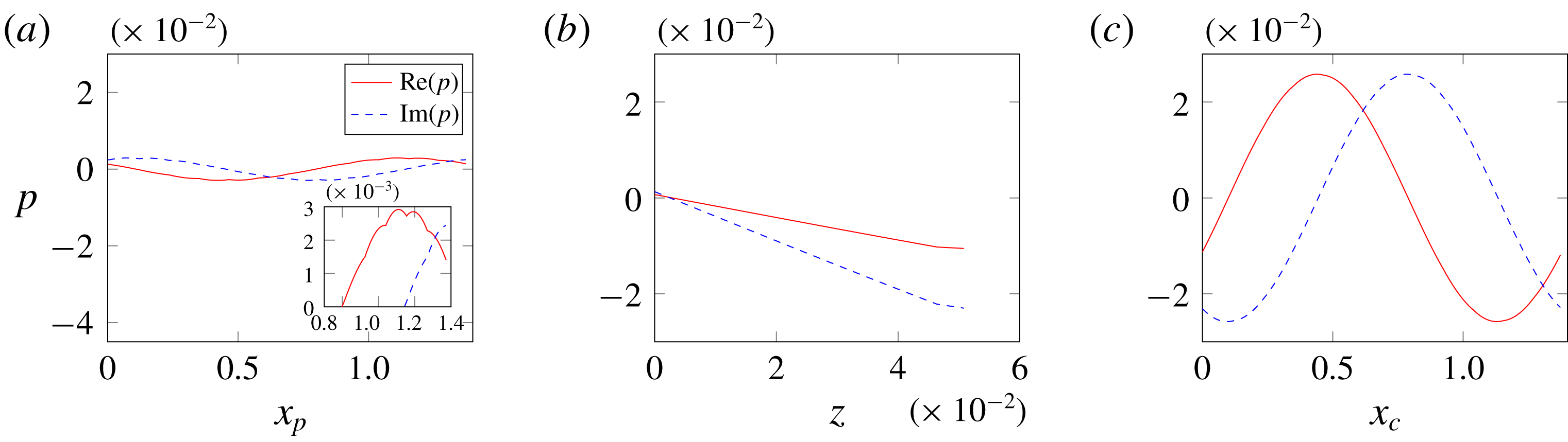
The spatial structure of the eigenmode on the brink of a Hopf bifurcation, corresponding to the root of unity
 $j=1$
, is visualized in figure 6(a–c). Figure 6(c) illustrates the structure of the mode along the perimeter of the annular chamber, figure 6(a) presents the modal shape along the perimeter of the annular plenum and figure 6(b) presents the variation in the burner. This eigenmode corresponds to a weakly coupled chamber (WCC) mode, based on the nomenclature used in Bauerheim et al. (Reference Bauerheim, Parmentier, Salas, Nicoud and Poinsot2014), and corresponds to the lowest-frequency globally periodic azimuthal eigenmode of the system (see figure 5
b) that also belongs to an eigenspace of dimension two (
 $j=1$
and
 $j=N-1$
). In addition, such modes exhibit a weak coupling between the chamber and plenum sections of the eigenmode, with the chamber section exhibiting the stronger response. Hence the cusps seen in figure 6(a), which are an artefact of the coupling between the two cavities, are too small to be noticed in the chamber mode in figure 6(c).
Structure of the eigenmode corresponding to the eigenvalue on the brink of undergoing a Hopf bifurcation, along the (a) plenum (b) burner and (c) chamber.

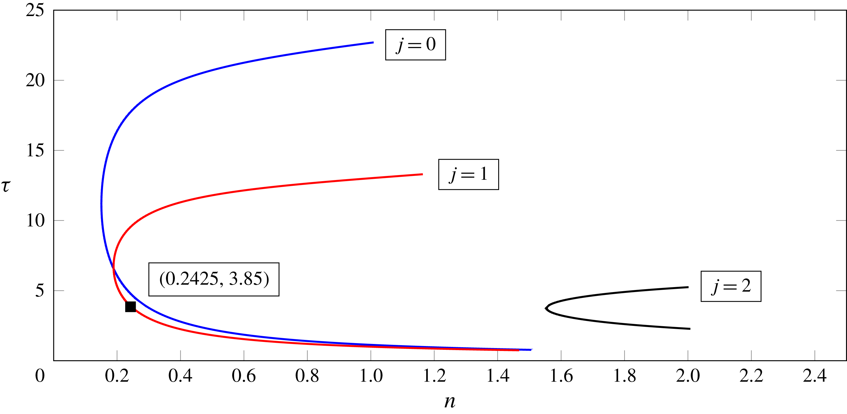
The neutral curves of this PBC system, displaying the linear stability boundaries as a function of the non-dimensional strength
 $n$
, time delay
 $\unicode[STIX]{x1D70F}$
and
 $j$
, for a fixed flame location are shown in figure 7. Each neutral curve in figure 7 represents the demarcation line across which an eigenmode, corresponding to a particular root of unit
 $j$
, will change from stable to unstable behaviour in the
 $(n,\unicode[STIX]{x1D70F})$
parameter space. Together, the neutral curves corresponding to
 $j=0$
and
 $j=1$
describe the positions of transition in linear stability, in the
 $(n,\unicode[STIX]{x1D70F})$
parameter space, for the system under consideration. The roots of unity corresponding to
 $j>2$
do not undergo a Hopf bifurcation in this portion of the
 $(n,\unicode[STIX]{x1D70F})$
-space and are therefore not shown in the figure. Global stability must account for all possible modes within the annular (periodic) domain. However, considering only a single sector with periodic boundary conditions (
 $j=0$
) will only represent a subset of the modes that may manifest themselves within the global domain. Hence a neutral curve corresponding to
 $j=0$
is not a global description of the system’s stability, as other globally periodic modes may undergo Hopf bifurcations before any mode corresponding to
 $j=0$
. This is evident from the more unstable behaviour of eigenmodes corresponding to the root of unity
 $j=1$
. Furthermore, this figure shows that stability limits according to individual neutral curves vary in relation to one another over the
 $(n,\unicode[STIX]{x1D70F})$
parameter space, leading to variations in modal structure (e.g. root-of-unity index
 $j$
) of the most unstable eigenmode as a function of the system parameters. A similar set of neutral curves (for a fixed flame location) indicating the nonlinear stability boundaries, as a function of
 $n$
,
 $\unicode[STIX]{x1D70F}$
and
 $j,$
can be constructed if the weakly nonlinear analysis performed in § 4.2 is continued to fifth order. This is required in order to obtain the point in parameter space where the roots of the resulting Stuart–Landau equation coalesce into a single value, representing the fold point or nonlinear stability boundary. However, recognizing the cumbersome derivation of the weakly nonlinear expansion (a drawback of the method) in case of degenerate modes, we have limited our analysis to a third-order, uniformly valid asymptotic expansion in § 4.2. Furthermore, a simpler third-order flame model is sufficient for the procedure mentioned in this manuscript; however, to aid future work that will continue the asymptotic expansion to higher orders we retain the fifth-order flame model in this work.
Neutral curve presented in the
 $(n,\unicode[STIX]{x1D70F})$
space for the PBC configuration. The black square represents the point in parameter space where the system will be studied. Here, the value of
 $z_{f}=0.88$
.

4.2 Weakly nonlinear analysis
We proceed by describing the conditions which allow broadband, environmental noise to pulse an annular PBC-type combustion chamber, from a stable base flow to a state of sustained oscillations, a process known as triggering (Sujith et al. Reference Sujith, Juniper and Schmid2016), by analysing the weakly nonlinear behaviour of the system close to the onset of linear instability (Hopf point) using the method of multiple scales. This method determines the nonlinear nature of the Hopf bifurcation and characterizes the branch of periodic solutions that emerge from the Hopf point in the form of a uniformly valid asymptotic expansion. This is achieved by introducing different time scales to formally separate the fast and slow system behaviour as described in Newell & Whitehead (Reference Newell and Whitehead1969), followed by the superposition of different spatial modes satisfying the system’s behaviour at each time scale, along with their corresponding time-varying amplitudes. The time-dependent amplitude evolution is described by ordinary differential equations, known as the Stuart–Landau (S–L) equations, that result from solvability conditions (Oden & Demkowicz Reference Oden and Demkowicz2017) for a uniformly valid asymptotic expansion. Finally, the fixed points of these S–L equations determine the amplitude and stability of steady and periodic solutions.
4.2.1 Asymptotic expansion
The equation describing the temporal evolution of thermo-acoustic instabilities in an annular combustion chamber, with
 $N$
identical sectors along the azimuthal direction, can be represented by
 $$\begin{eqnarray}\dot{\boldsymbol{x}}(t)=\unicode[STIX]{x1D63C}\,\boldsymbol{x}(t)+n\mathop{\sum }_{m=1}^{N}\boldsymbol{B}_{m}\mathop{\sum }_{i=1}^{5}\unicode[STIX]{x1D6FC}_{i}(\boldsymbol{C}_{m}\boldsymbol{x}(t-\unicode[STIX]{x1D70F}))^{i},\end{eqnarray}$$
where
 $\boldsymbol{x}$
is the global state vector of the entire
 $N$
-periodic geometry (a union of
 $\boldsymbol{x}_{us}$
from each unit-sector), and
 $\unicode[STIX]{x1D63C}$
is the respective global
 $N$
-periodic block-circulant acoustic operator. The term
 $\unicode[STIX]{x1D6FC}_{i}$
represents the coefficients of the nonlinear flame model, as mentioned in (2.4),
 $n$
is the flame strength parameter and
 $\unicode[STIX]{x1D70F}$
is the flame delay parameter. Column vector
 $\boldsymbol{B}_{m}$
and row vector
 $\boldsymbol{C}_{m}$
represent the vectors that select the pressure point at which the compact nonlinear flame model is imposed and the velocity point at which the upstream velocity is measured, respectively. The roots-of-unity modified unit-sector version of (4.1) is given by (3.6). Equation (4.1) is simply a convenient form for the asymptotic analysis.
Once a dynamical system goes through a Hopf bifurcation the existing perturbations are prone to grow and saturate into a limit cycle due to the existence of higher-order nonlinear terms. If the system exhibits a subcritical bifurcation, then there exists a bistable region ahead of the Hopf point where stable solutions with finite-amplitude oscillations appear. The amplitude of these oscillations is extracted using a weakly nonlinear analysis where the governing equation is expanded about the Hopf point, leading to an expansion of the following form
 $$\begin{eqnarray}\boldsymbol{x}=\unicode[STIX]{x1D716}\boldsymbol{x}_{1}+\unicode[STIX]{x1D716}^{2}\boldsymbol{x}_{2}+\unicode[STIX]{x1D716}^{3}\boldsymbol{x}_{3}+\cdots\end{eqnarray}$$
where
 $0<\unicode[STIX]{x1D716}\ll 1$
. The bifurcation parameter is also perturbed around its critical value
 $n=n^{c}+\unicode[STIX]{x0394}n$
, where
 $|\unicode[STIX]{x0394}n|\ll 1$
. Similar to Orchini et al. (Reference Orchini, Rigas and Juniper2016), the method of multiple scales is then employed, where independent time scales are assumed to be present simultaneously. The fast time scale
 $t_{0}$
is associated with oscillations of the marginally stable frequency, whereas, time scale
 $t_{2}$
applies to long-time saturation or growth processes, resulting in
 $$\begin{eqnarray}\dot{\boldsymbol{x}}=\frac{\unicode[STIX]{x2202}\boldsymbol{x}}{\unicode[STIX]{x2202}t_{0}}+\unicode[STIX]{x1D716}^{2}\frac{\unicode[STIX]{x2202}\boldsymbol{x}}{\unicode[STIX]{x2202}t_{2}},\end{eqnarray}$$
where the choice of
 $\unicode[STIX]{x1D716}$
exponent is informed by the requirement that the asymptotic expansion be uniformly valid.
Applying (4.3) to governing equations (4.1), we obtain a Taylor expansion of the dynamical system around the fixed point solution
 $\boldsymbol{x}=0$
, at the critical flame strength
 $n^{c}$
(Hopf point), as follows
 $$\begin{eqnarray}\displaystyle \frac{\unicode[STIX]{x2202}\boldsymbol{x}}{\unicode[STIX]{x2202}t_{0}}+\unicode[STIX]{x1D716}^{2}\frac{\unicode[STIX]{x2202}\boldsymbol{x}}{\unicode[STIX]{x2202}t_{2}} & = & \displaystyle \unicode[STIX]{x1D63C}\,\boldsymbol{x}(t)+n^{c}\mathop{\sum }_{m=1}^{N}\boldsymbol{B}_{m}\mathop{\sum }_{i=1}^{5}\unicode[STIX]{x1D6FC}_{i}(\boldsymbol{C}_{m}\boldsymbol{x}(t-\unicode[STIX]{x1D70F}))^{i}\nonumber\\ \displaystyle & & \displaystyle +\,\unicode[STIX]{x0394}n\mathop{\sum }_{m=1}^{N}\boldsymbol{B}_{m}\mathop{\sum }_{i=1}^{5}\unicode[STIX]{x1D6FC}_{i}(\boldsymbol{C}_{m}\boldsymbol{x}(t-\unicode[STIX]{x1D70F}))^{i},\end{eqnarray}$$
where
 $\unicode[STIX]{x1D716}\approx 10^{-2}$
and
 $\unicode[STIX]{x0394}n=\unicode[STIX]{x1D716}^{2}\unicode[STIX]{x1D6FF}_{2}$
is the
 $\unicode[STIX]{x1D716}^{2}$
-order change in the flame strength parameter (Orchini et al.
Reference Orchini, Rigas and Juniper2016). The term
 $\unicode[STIX]{x1D6FF}_{2}$
can take values
 $\pm 1$
depending on the direction in which the critical parameter (
 $n$
) is perturbed. This order of change in the flame strength parameter is chosen so as to obtain control parameters that help enforce solvability conditions (removal of secular forcing terms), which guarantee the validity of the asymptotic expansion at larger time scales. In the case of a subcritical bifurcation, an expansion up to third order resolves oscillations on the unstable branch of the bifurcation diagram; however, these solutions are unobservable in experiments. In cases where stable limit cycles prior to the Hopf point are of interest, an expansion up to fifth order is required (Orchini et al.
Reference Orchini, Rigas and Juniper2016). Since, the objective of this study is to illustrate the presence of a subcritical bifurcation only, a fifth-order expansion is not considered. In the following sections we solve for each term in the asymptotic expansion mentioned in (4.2) one order at a time.
4.2.2
 $O(\unicode[STIX]{x1D716})$
: eigenvalue problem

Collecting
 $O(\unicode[STIX]{x1D716})$
terms of (4.4) results in the linearized version of (4.1),
 $$\begin{eqnarray}\frac{\unicode[STIX]{x2202}\boldsymbol{x}_{1}}{\unicode[STIX]{x2202}t_{0}}-\unicode[STIX]{x1D63C}\,\boldsymbol{x}_{1}-\mathop{\sum }_{m=1}^{N}\unicode[STIX]{x1D6FC}_{1}n^{c}\boldsymbol{B}_{m}(\boldsymbol{C}_{m}\boldsymbol{x}_{1}(t-\unicode[STIX]{x1D70F}))=0.\end{eqnarray}$$
In order to simplify the notation, an operator
 $\unicode[STIX]{x1D648}_{s}$
is defined in the spectral domain (
 $s$
is the Laplace variable), and is given by
 $$\begin{eqnarray}\unicode[STIX]{x1D648}_{s}=s\unicode[STIX]{x1D644}-\unicode[STIX]{x1D63C}-\unicode[STIX]{x1D6FC}_{1}n^{c}\mathop{\sum }_{m=1}^{N}\boldsymbol{B}_{m}\otimes \boldsymbol{C}_{m}\text{e}^{-s\unicode[STIX]{x1D70F}}.\end{eqnarray}$$
Using
 $\unicode[STIX]{x1D648}_{s}$
, equation (4.5) can be reformulated as the following nonlinear eigenvalue problem
 $\unicode[STIX]{x1D648}_{s}\boldsymbol{x}_{1}=0$
. The values of
 $s$
that satisfy this problem are computed using the PDE method presented in § 3.4. Since each operator
 $\unicode[STIX]{x1D644}$
,
 $\unicode[STIX]{x1D63C}$
and
 $\boldsymbol{B}_{m}\otimes \boldsymbol{C}_{m}$
is individually block circulant,
 $\unicode[STIX]{x1D648}_{s}$
becomes a block-circulant operator as well. The analysis presented in Schmid et al. (Reference Schmid, Fosas de Pando and Peake2017), shows that
 $\unicode[STIX]{x1D648}_{s}$
can be transformed into a block diagonal form through a similarity transformation. Thus a block-circulant matrix,
 $\unicode[STIX]{x1D648}_{s}$
, with degenerate eigenvalues, is recast as
 $N$
root-of-unity matrices (with
 $N$
unique blocks in the block-circulant structure of the direct matrix), each with an eigenspectrum of algebraic multiplicity one. Amongst these
 $N$
operators, there exist
 $N/2-1$
or
 $(N-1)/2$
pairs of operators that share the same eigenspectrum when
 $N$
is even or odd, on account of the discrete rotational symmetry associated with the
 $N$
-periodic geometry of the annular combustion chamber (Salas Reference Salas2013). Since the eigenspectrum of the global block-circulant operator is the union of eigenspectra from each linearly independent root-of-unity operator, the global operator must also have degenerate eigenvalues with a maximum algebraic multiplicity of two, in cases where the eigenvalue is non-zero. This implies that the eigenvalue problem in (4.5) is simultaneously satisfied by two mutually orthogonal eigenvectors corresponding to two different root-of-unity operators. In other words, any linear combination of the eigenvectors from the root-of-unity operators corresponding to
 $j$
and
 $N-j$
, that share the same eigenvalue on the verge of a Hopf bifurcation, will also satisfy (4.5). For more details regarding the degenerate behaviour of such systems, the reader is referred to Salas (Reference Salas2013).
This degeneracy is known to exist for such annular systems, as observed by Ghirardo et al. (Reference Ghirardo, Juniper and Moeck2016), where a pair of orthogonal standing modes is used to illustrate the importance of accounting for degenerate eigenmodes in explaining the rich dynamical features, such as spinning, standing and mixed-mode limit cycles, in a similar annular configuration. While multiple time scale analysis has been performed in the past to include nonlinearities in thermo-acoustic systems, such as the work of Orchini et al. (Reference Orchini, Rigas and Juniper2016), it has mainly focused on longitudinal burner configurations, where degenerate waves of the non-defective type are absent. Therefore, the analysis described in Orchini et al. (Reference Orchini, Rigas and Juniper2016) needs to be modified to include degeneracies in order to be applicable to annular geometries. This modification is achieved by constructing a unique pair of orthogonal eigenvectors
 $\boldsymbol{x}_{1}^{W}$
and
 $\boldsymbol{x}_{1}^{Z}$
, using the two root-of-unity operators which share the eigenvalue of the global matrix,
 $\unicode[STIX]{x1D648}_{s}$
, close to a Hopf bifurcation (
 $s=\text{i}\unicode[STIX]{x1D714}^{c}$
). The resulting pair of eigenvectors span the space of all vectors satisfying (4.5) through the following expression,
 $$\begin{eqnarray}\boldsymbol{x}_{1}=(W(t_{2})\boldsymbol{x}_{1}^{W}\text{e}^{\text{i}\unicode[STIX]{x1D714}^{c}t_{0}}+\text{c.c.})+(Z(t_{2})\boldsymbol{x}_{1}^{Z}\text{e}^{\text{i}\unicode[STIX]{x1D714}^{c}t_{0}}+\text{c.c.}),\end{eqnarray}$$
where
 $W$
and
 $Z$
are the slowly varying amplitudes of the orthogonal vectors
 $\boldsymbol{x}_{1}^{W}$
and
 $\boldsymbol{x}_{1}^{Z}$
, respectively. Accounting for a pair of orthogonal eigenvectors rather than a single eigenvector, and the subsequent computation of the higher-order terms incorporates the inherent degeneracy into the final, uniformly valid asymptotic analysis.
4.2.3
$O(\unicode[STIX]{x1D716}^{2})$
: mean shift and second harmonic

At this order we obtain the equations for the evolution of
 $\boldsymbol{x}_{2}$
. From here onwards, forcing terms appear on the right-hand-side of the equations. These forcing terms are due to interactions between solutions
 $\boldsymbol{x}_{k}$
, where
 $k<{\mathcal{M}}$
, and
 ${\mathcal{M}}$
is the order of the expansion. The only forcing term at this order is
 $\unicode[STIX]{x1D6F4}_{m=1}^{N}\unicode[STIX]{x1D6FC}_{2}n^{c}\boldsymbol{B}_{m}(\boldsymbol{C}_{m}\boldsymbol{x}_{1}(t-\unicode[STIX]{x1D70F}))^{2}$
, which is further expanded, using (4.7), to obtain the following
 $O(\unicode[STIX]{x1D716}^{2})$
inhomogeneous linear component of (4.1)
 $$\begin{eqnarray}\displaystyle & & \displaystyle \frac{\unicode[STIX]{x2202}\boldsymbol{x}_{2}}{\unicode[STIX]{x2202}t_{0}}-\unicode[STIX]{x1D63C}\,\boldsymbol{x}_{2}-\mathop{\sum }_{m=1}^{N}\unicode[STIX]{x1D6FC}_{1}n^{c}\boldsymbol{B}_{m}(\boldsymbol{C}_{m}\boldsymbol{x}_{2}(t-\unicode[STIX]{x1D70F}))\nonumber\\ \displaystyle & & \displaystyle \quad =\mathop{\sum }_{m=1}^{N}\unicode[STIX]{x1D6FC}_{2}n^{c}\boldsymbol{B}_{m}(\boldsymbol{C}_{m}((W(t_{2})\boldsymbol{x}_{1}^{W}\text{e}^{\text{i}\unicode[STIX]{x1D714}^{c}t_{0}}+\text{c.c.})\nonumber\\ \displaystyle & & \displaystyle \qquad +\,(Z(t_{2})\boldsymbol{x}_{1}^{Z}\text{e}^{\text{i}\unicode[STIX]{x1D714}^{c}t_{0}}+\text{c.c.})))^{2}\end{eqnarray}$$
 $$\begin{eqnarray}\displaystyle & & \displaystyle \quad =|W|^{2}\left(\mathop{\sum }_{m=1}^{N}\boldsymbol{F}_{2,m}^{|W|^{2}}\right)+\left(W^{2}\left(\mathop{\sum }_{m=1}^{N}\boldsymbol{F}_{2,m}^{W^{2}}\right)\text{e}^{2\text{i}\unicode[STIX]{x1D714}^{c}t_{0}}+\text{c.c.}\right)\nonumber\\ \displaystyle & & \displaystyle \qquad +\,|Z|^{2}\left(\mathop{\sum }_{m=1}^{N}\boldsymbol{F}_{2,m}^{|Z|^{2}}\right)+\left(ZW^{\ast }\left(\mathop{\sum }_{m=1}^{N}\boldsymbol{F}_{2,m}^{ZW^{\ast }}\right)+\text{c.c.}\right)\nonumber\\ \displaystyle & & \displaystyle \qquad +\,\left(Z^{2}\left(\mathop{\sum }_{m=1}^{N}\boldsymbol{F}_{2,m}^{Z^{2}}\right)\text{e}^{2\text{i}\unicode[STIX]{x1D714}^{c}t_{0}}+\text{c.c.}\right)\nonumber\\ \displaystyle & & \displaystyle \qquad +\,\left(WZ\left(\mathop{\sum }_{m=1}^{N}\boldsymbol{F}_{2,m}^{WZ}\right)\text{e}^{2\text{i}\unicode[STIX]{x1D714}^{c}t_{0}}+\text{c.c.}\right),\end{eqnarray}$$
 $\boldsymbol{x}_{1}$
. Explicit expressions for the forcing terms are relegated to § B.1. The last four terms on the right-hand side of (4.8) are added to the expression derived by Orchini et al. (Reference Orchini, Rigas and Juniper2016) due to the presence of degeneracy in the annular system. The first two of these terms are modifications to the steady-state forcing, with zero frequency, while the last two represent contribution to the second harmonic. A steady-state solution
 $\boldsymbol{x}_{2}$
, with the same shape as the forcing, can be extracted by using the ansatz,
 $$\begin{eqnarray}\displaystyle \boldsymbol{x}_{2} & = & \displaystyle |W|^{2}(\boldsymbol{x}_{2}^{|W|^{2}})+(W^{2}(\boldsymbol{x}_{2}^{W^{2}})\text{e}^{2\text{i}\unicode[STIX]{x1D714}^{c}t_{0}}+\text{c.c.})\nonumber\\ \displaystyle & & \displaystyle +\,|Z|^{2}(\boldsymbol{x}_{2}^{|Z|^{2}})+(Z^{2}(\boldsymbol{x}_{2}^{Z^{2}})\text{e}^{2\text{i}\unicode[STIX]{x1D714}^{c}t_{0}}+\text{c.c.})\nonumber\\ \displaystyle & & \displaystyle +\,(ZW^{\ast }(\boldsymbol{x}_{2}^{ZW^{\ast }})+\text{c.c.})+(ZW(\boldsymbol{x}_{2}^{ZW})\text{e}^{2\text{i}\unicode[STIX]{x1D714}^{c}t_{0}}+\text{c.c.}).\end{eqnarray}$$
Substituting this expression into (4.8) and computing each term on the right-hand side in the spectral domain gives,
 $$\begin{eqnarray}\left(s\unicode[STIX]{x1D644}-\unicode[STIX]{x1D63C}-\mathop{\sum }_{m=1}^{N}\unicode[STIX]{x1D6FC}_{1}n^{c}\boldsymbol{B}_{m}(\boldsymbol{C}_{m}\boldsymbol{x}_{1}\text{e}^{-s\unicode[STIX]{x1D70F}})\right)\boldsymbol{x}_{2}^{a}\text{e}^{st_{0}}=\unicode[STIX]{x1D648}_{s}\boldsymbol{x}_{2}^{a}\text{e}^{st_{0}}=\mathop{\sum }_{m=1}^{N}\boldsymbol{F}_{2,m}^{a}\text{e}^{st_{0}},\end{eqnarray}$$
where
 $a$
is a general representation of the amplitude-based classification of the terms in the steady-state ansatz,
 $\boldsymbol{F}_{2,m}^{a}$
represents the amplitude based classification of the right-hand side forcing terms in (4.8b
) and
 $s$
is the corresponding frequency associated with that term. The matrix
 $\unicode[STIX]{x1D648}_{s}$
on the left-hand side is non-singular if
 $s=2\text{i}\unicode[STIX]{x1D714}^{c}$
as this is not an eigenvalue of the linear acoustic operator
 $\unicode[STIX]{x1D63C}$
. In case of a constant mode (with zero frequency), the Moore–Penrose inverse is used when evaluating (4.10), to ensure that the summation over the force terms is orthogonal to the null space of the adjoint of
 $\unicode[STIX]{x1D648}_{0}$
.
4.2.4
$O(\unicode[STIX]{x1D716}^{3})$
: third harmonic and saturation

At this order the equations for the evolution of
 $\boldsymbol{x}_{3}$
are obtained. We have
 $$\begin{eqnarray}\displaystyle & & \displaystyle \frac{\unicode[STIX]{x2202}\boldsymbol{x}_{3}}{\unicode[STIX]{x2202}t_{0}}-\unicode[STIX]{x1D63C}\,\boldsymbol{x}_{3}-\mathop{\sum }_{m=1}^{N}\unicode[STIX]{x1D6FC}_{1}n^{c}\boldsymbol{B}_{m}(\boldsymbol{C}_{m}\boldsymbol{x}_{3}(t-\unicode[STIX]{x1D70F}))\nonumber\\ \displaystyle & & \displaystyle \quad =-\frac{\unicode[STIX]{x2202}\boldsymbol{x}_{1}}{\unicode[STIX]{x2202}t_{2}}-\unicode[STIX]{x1D70F}\mathop{\sum }_{m=1}^{N}\unicode[STIX]{x1D6FC}_{1}n^{c}\boldsymbol{B}_{m}\left(\boldsymbol{C}_{m}\frac{\unicode[STIX]{x2202}\boldsymbol{x}_{1}}{\unicode[STIX]{x2202}t_{2}}(t-\unicode[STIX]{x1D70F})\right)\nonumber\\ \displaystyle & & \displaystyle \qquad +\,(\boldsymbol{F}_{\unicode[STIX]{x1D714}^{c}}(\boldsymbol{x}_{1},\boldsymbol{x}_{2})\text{e}^{\text{i}\unicode[STIX]{x1D714}^{c}t_{0}}+\boldsymbol{F}_{3\unicode[STIX]{x1D714}^{c}}(\boldsymbol{x}_{1},\boldsymbol{x}_{2})\text{e}^{3\text{i}\unicode[STIX]{x1D714}^{c}t_{0}}+\text{c.c.}).\end{eqnarray}$$
Following the procedure from the previous section, expressions in (4.7) and (4.9) are used to obtain an amplitude-based classification of the forcing terms as demonstrated in § B.2. Explicit expressions for the forcing terms are also relegated to § B.2.
Forcing terms corresponding to the angular frequency
 $\unicode[STIX]{x1D714}^{c}$
(B 2) lead to resonant forcing at eight different amplitude levels, namely
 $W$
,
 $|W|^{2}W$
,
 $Z$
,
 $|Z|^{2}Z$
,
 $|W|^{2}Z$
,
 $|Z|^{2}W$
,
 $W^{2}Z^{\ast }$
and
 $Z^{2}W^{\ast }$
. Hence, a solvability condition – also known as the Fredholm alternative (Oden & Demkowicz Reference Oden and Demkowicz2017) – needs to be satisfied in order for a uniformly valid, asymptotic solution to exist. This solvability condition requires the sum of the resonant forcing terms to be orthogonal to the kernel of the adjoint matrix
 $\unicode[STIX]{x1D648}_{\text{i}\unicode[STIX]{x1D714}^{c}}^{+}$
(Sipp & Lebedev Reference Sipp and Lebedev2007). This procedure generalizes the idea of cancelling the secular terms, employed for weakly nonlinear analysis of scalar problems (Orchini et al.
Reference Orchini, Rigas and Juniper2016).
In order to derive this solvability condition, a set of unique vectors spanning the null space of the Hermitian of the direct matrix
 $\unicode[STIX]{x1D648}_{\text{i}\unicode[STIX]{x1D714}^{c}}$
, or in other words its adjoint, are required. The direct matrix under consideration is known to have eigenvalues that have an algebraic multiplicity of two and is block circulant, thus ensuring its adjoint (Hermitian) shares these properties. The equivalent procedure that was used to determine
 $\boldsymbol{x}_{1}^{W}$
and
 $\boldsymbol{x}_{1}^{Z}$
is employed to construct a pair of orthogonal eigenvectors, denoted by
 $\boldsymbol{x}_{1}^{W+}$
and
 $\boldsymbol{x}_{1}^{Z+}$
, associated with the null space of the adjoint matrix, by simply considering the eigenvectors of the Hermitian of the two root-of-unity matrices, used to obtain
 $\boldsymbol{x}_{1}^{W}$
and
 $\boldsymbol{x}_{1}^{Z}$
. Applying this solvability condition, described in detail in appendix C, leads to the following coupled equations describing the evolution of the complex amplitudes
 $W$
and
 $Z$
:
 $$\begin{eqnarray}\displaystyle \unicode[STIX]{x1D6FD}_{\unicode[STIX]{x2202}W}\frac{\unicode[STIX]{x2202}W}{\unicode[STIX]{x2202}t_{2}}+\unicode[STIX]{x1D6FD}_{\unicode[STIX]{x2202}Z}\frac{\unicode[STIX]{x2202}Z}{\unicode[STIX]{x2202}t_{2}} & = & \displaystyle \unicode[STIX]{x1D6FD}_{W}W+\unicode[STIX]{x1D6FD}_{|W|^{2}W}|W|^{2}W+\unicode[STIX]{x1D6FD}_{Z}Z+\unicode[STIX]{x1D6FD}_{|Z|^{2}Z}|Z|^{2}Z+\unicode[STIX]{x1D6FD}_{|W|^{2}Z}|W|^{2}Z\nonumber\\ \displaystyle & & \displaystyle +\,\unicode[STIX]{x1D6FD}_{|Z|^{2}W}|Z|^{2}W+\unicode[STIX]{x1D6FD}_{W^{2}Z^{\ast }}W^{2}Z^{\ast }+\unicode[STIX]{x1D6FD}_{Z^{2}W^{\ast }}Z^{2}W^{\ast },\end{eqnarray}$$
 $$\begin{eqnarray}\displaystyle \unicode[STIX]{x1D6FE}_{\unicode[STIX]{x2202}W}\frac{\unicode[STIX]{x2202}W}{\unicode[STIX]{x2202}t_{2}}+\unicode[STIX]{x1D6FE}_{\unicode[STIX]{x2202}Z}\frac{\unicode[STIX]{x2202}Z}{\unicode[STIX]{x2202}t_{2}} & = & \displaystyle \unicode[STIX]{x1D6FE}_{W}W+\unicode[STIX]{x1D6FE}_{|W|^{2}W}|W|^{2}W+\unicode[STIX]{x1D6FE}_{Z}Z+\unicode[STIX]{x1D6FE}_{|Z|^{2}Z}|Z|^{2}Z+\unicode[STIX]{x1D6FE}_{|W|^{2}Z}|W|^{2}Z\nonumber\\ \displaystyle & & \displaystyle +\,\unicode[STIX]{x1D6FE}_{|Z|^{2}W}|Z|^{2}W+\unicode[STIX]{x1D6FE}_{W^{2}Z^{\ast }}W^{2}Z^{\ast }+\unicode[STIX]{x1D6FE}_{Z^{2}W^{\ast }}Z^{2}W^{\ast }.\end{eqnarray}$$
The coefficients
 $\unicode[STIX]{x1D6FD}_{a}$
(or
 $\unicode[STIX]{x1D6FE}_{a}$
) are given as the inner products between
 $\boldsymbol{x}_{1}^{W+}$
(or
 $\boldsymbol{x}_{1}^{Z+}$
) and
 $\sum _{m=1}^{N}\boldsymbol{F}_{3,m}^{a}$
where
 $a$
is a general representation of the subscripts of
 $\unicode[STIX]{x1D6FD}$
and
 $\unicode[STIX]{x1D6FE}$
(in the above equations the
 $\unicode[STIX]{x2202}$
symbol in the subscript is used only for the purpose of notation). The exact expressions for each
 $\unicode[STIX]{x1D6FD}_{a}$
and
 $\unicode[STIX]{x1D6FE}_{a}$
term is given in (C 1a
) and (C 1b
), respectively.
4.2.5 Stuart–Landau equation at
$O(\unicode[STIX]{x1D716}^{3})$
and flame model

Equations (4.12a
) are known as Stuart–Landau equations. Together, these equations yield the amplitude of limit-cycle solutions and the frequency shift (not mentioned here) of the nonlinear oscillation with respect to the marginally stable eigenfrequency. In other words, these equations help identify the nonlinear mechanism which describes the finite-amplitude thermo-acoustic oscillations in annular combustors by providing ordinary differential equations (ODEs) that describe the temporal variation of the complex amplitudes
 $W(t_{2})$
and
 $Z(t_{2})$
.
Using a polar representation
 $W=r_{W}\text{e}^{\text{i}\unicode[STIX]{x1D703}_{W}}$
,
 $Z=r_{Z}\text{e}^{\text{i}\unicode[STIX]{x1D703}_{Z}}$
and observing that the terms
 $\unicode[STIX]{x1D6FD}_{\unicode[STIX]{x2202}Z}$
,
 $\unicode[STIX]{x1D6FE}_{\unicode[STIX]{x2202}W}$
,
 $\unicode[STIX]{x1D6FD}_{Z}$
and
 $\unicode[STIX]{x1D6FE}_{W}$
are zero on account of the different root-of-unity indices used to construct the global versions of these vectors gives
 $$\begin{eqnarray}\displaystyle \frac{\unicode[STIX]{x2202}r_{W}}{\unicode[STIX]{x2202}t_{2}} & = & \displaystyle \text{Re}\left(\frac{\unicode[STIX]{x1D6FD}_{W}}{\unicode[STIX]{x1D6FD}_{\unicode[STIX]{x2202}W}}\right)r_{W}+\text{Re}\left(\frac{\unicode[STIX]{x1D6FD}_{|W|^{2}W}}{\unicode[STIX]{x1D6FD}_{\unicode[STIX]{x2202}W}}\right)r_{W}^{3}+\text{Re}\left(\frac{\unicode[STIX]{x1D6FD}_{|Z|^{2}Z}}{\unicode[STIX]{x1D6FD}_{\unicode[STIX]{x2202}W}}\right)r_{Z}^{3}+\text{Re}\left(\frac{\unicode[STIX]{x1D6FD}_{|W|^{2}Z}}{\unicode[STIX]{x1D6FD}_{\unicode[STIX]{x2202}W}}\right)r_{W}^{2}r_{Z}\nonumber\\ \displaystyle & & \displaystyle +\,\text{Re}\left(\frac{\unicode[STIX]{x1D6FD}_{|Z|^{2}W}}{\unicode[STIX]{x1D6FD}_{\unicode[STIX]{x2202}W}}\right)r_{Z}^{2}r_{W}+\text{Re}\left(\frac{\unicode[STIX]{x1D6FD}_{W^{2}Z^{\ast }}}{\unicode[STIX]{x1D6FD}_{\unicode[STIX]{x2202}W}}\right)r_{W}^{2}r_{Z}+\text{Re}\left(\frac{\unicode[STIX]{x1D6FD}_{Z^{2}W^{\ast }}}{\unicode[STIX]{x1D6FD}_{\unicode[STIX]{x2202}W}}\right)r_{Z}^{2}r_{W},\end{eqnarray}$$
 $$\begin{eqnarray}\displaystyle \frac{\unicode[STIX]{x2202}r_{Z}}{\unicode[STIX]{x2202}t_{2}} & = & \displaystyle \text{Re}\left(\frac{\unicode[STIX]{x1D6FE}_{Z}}{\unicode[STIX]{x1D6FE}_{\unicode[STIX]{x2202}Z}}\right)r_{Z}+\text{Re}\left(\frac{\unicode[STIX]{x1D6FE}_{|W|^{2}W}}{\unicode[STIX]{x1D6FE}_{\unicode[STIX]{x2202}Z}}\right)r_{W}^{3}+\text{Re}\left(\frac{\unicode[STIX]{x1D6FE}_{|Z|^{2}Z}}{\unicode[STIX]{x1D6FE}_{\unicode[STIX]{x2202}Z}}\right)r_{Z}^{3}+\text{Re}\left(\frac{\unicode[STIX]{x1D6FE}_{|W|^{2}Z}}{\unicode[STIX]{x1D6FE}_{\unicode[STIX]{x2202}Z}}\right)r_{W}^{2}r_{Z}\nonumber\\ \displaystyle & & \displaystyle +\,\text{Re}\left(\frac{\unicode[STIX]{x1D6FE}_{|Z|^{2}W}}{\unicode[STIX]{x1D6FE}_{\unicode[STIX]{x2202}Z}}\right)r_{Z}^{2}r_{W}+\text{Re}\left(\frac{\unicode[STIX]{x1D6FE}_{W^{2}Z^{\ast }}}{\unicode[STIX]{x1D6FE}_{\unicode[STIX]{x2202}Z}}\right)r_{W}^{2}r_{Z}+\text{Re}\left(\frac{\unicode[STIX]{x1D6FE}_{Z^{2}W^{\ast }}}{\unicode[STIX]{x1D6FE}_{\unicode[STIX]{x2202}Z}}\right)r_{Z}^{2}r_{W}.\end{eqnarray}$$
 $r_{W}$
and
 $r_{Z}$
in the asymptotic limit
 $t_{2}\rightarrow \infty$
; in other words the roots of the above equations are the steady-state or periodic solutions of the underlying dynamical system. Amplitudes found with
 $\text{sign}(\unicode[STIX]{x0394}n)=\unicode[STIX]{x1D6FF}_{2}=-1$
signify a subcritical bifurcation and those found with
 $\text{sign}(\unicode[STIX]{x0394}n)=\unicode[STIX]{x1D6FF}_{2}=1$
describe a supercritical bifurcation. We recall that
 $\unicode[STIX]{x1D6FF}_{2}$
is the sign associated with the modification of parameter
 $n;$
thus if we locate a limit cycle when
 $\unicode[STIX]{x1D6FF}_{2}<0$
(
 $\unicode[STIX]{x1D6FF}_{2}>0$
) the bifurcation must be subcritical (supercritical). In the case of a subcritical (supercritical) bifurcation, the extracted amplitude corresponds to an unstable (stable) limit cycle, when the weakly nonlinear asymptotic expansion is truncated at
 $O(\unicode[STIX]{x1D716}^{3})$
. As mentioned previously, to compute the amplitude of a stable limit cycle in case of a subcritical bifurcation, the weakly nonlinear expansion must include fourth- and fifth-order terms.
At this stage, the neutral curve displayed in figure 7 can further be analysed to determine the nature of the bifurcation by studying the roots of its representative Stuart–Landau equation. However, in order to perform the weakly nonlinear expansion, a suitable nonlinear flame model needs to be selected. This flame model is derived using the same least-squares procedure described in Orchini et al. (Reference Orchini, Rigas and Juniper2016), approximating the saturation-type nonlinearity displayed by King’s law, as illustrated in figure 8. The flame model coefficients used to generate this comparison were given in equation set (2.5). This model is similar to the flame model used in Orchini et al. (Reference Orchini, Rigas and Juniper2016), with a slightly different domain. In our study, the domain
 $[-1.839,1.839]$
is chosen. This domain is sufficiently wide to include the saturation mechanism for amplitudes much higher than those that will be considered in this study. Figure 8(a) shows that the least-square fit model has the same linear behaviour as the unsteady King’s law and a qualitatively similar nonlinear behaviour, with a smooth saturation mechanism. When displaying the gain
 $G$
, shown in figure 8(b), the gain monotonically decreases with the amplitude forcing, except for a small region of
 $u/\tilde{u} <0.2$
, where the value slightly increases. The modest gain at small velocity amplitudes promotes the occurrence of a subcritical bifurcation over the portion of the neutral curve, corresponding to root-of-unity index
 $j=1$
, displayed in figure 11.
(a) Comparison of flame response from the least-squares flame model (red) to that of King’s law (black). (b) Gain of the flame model as a function of the velocity perturbation magnitudes, (red) signifies the portion with gain larger than unity. Here,
 $w_{f}$
is the velocity perturbation upstream (cold side) of the flame.

4.2.6 Weakly nonlinear analysis of the Hopf bifurcation
We then apply the weakly nonlinear analysis to the annular PBC configuration, described in § 2, in order to ascertain the nature of the system’s Hopf bifurcation and hence the evolution of finite-amplitude thermo-acoustic instabilities. At first, we focus on the weakly nonlinear behaviour at a single point adjacent to the neutral curve, with parameter values of
 $n=0.2425-\unicode[STIX]{x1D716}^{2}$
, and
 $\unicode[STIX]{x1D70F}=3.85$
, where
 $\unicode[STIX]{x1D716}=10^{-3}.$
As mentioned in § 4.3, in
 $(n,\unicode[STIX]{x1D70F})$
space this point lies a distance of
 $\unicode[STIX]{x1D716}^{2}$
to the left of the black square in figure 7 and corresponds to the location where non-modal instabilities of the PBC system have been analysed. Figure 9 shows a phase portrait of the temporally evolving finite-amplitude perturbations, along with the roots of the underlying Stuart–Landau equation for the selected configuration. The point at the origin represents the steady-state solution of the system, illustrated by the converging streamlines in its vicinity, whereas the other two points indicate a pair of spinning modes. Figure 9 shows that, close to these periodic solutions, finite-amplitude perturbations are both attracted and repelled. This is characteristic of a saddle-type finite-amplitude perturbation or a limit cycle, revealing the bi-stable nature of the system’s behaviour close to its neutral curve. The amplitude of the resulting unstable limit cycle, reported in the form of the axial velocity perturbations upstream of the flame, can now be extracted using the fixed point values of
 $r_{W}$
and
 $r_{Z}$
as
 $$\begin{eqnarray}|\boldsymbol{C}_{1}\boldsymbol{\cdot }\boldsymbol{x}|=|\boldsymbol{C}_{1}\boldsymbol{\cdot }(\unicode[STIX]{x1D716}\boldsymbol{x}_{1}(W,Z)+\unicode[STIX]{x1D716}^{2}\boldsymbol{x}_{2}(W,Z)+\unicode[STIX]{x1D716}^{3}\boldsymbol{x}_{3}(W,Z))|,\end{eqnarray}$$
where,
 $W=r_{W}\text{e}^{\text{i}\unicode[STIX]{x1D703}_{W}}$
,
 $Z=r_{Z}\text{e}^{\text{i}\unicode[STIX]{x1D703}_{Z}}$
and,
 $\boldsymbol{x}_{1}(W,Z)$
,
 $\boldsymbol{x}_{2}(W,Z)$
and
 $\boldsymbol{x}_{3}(W,Z)$
are given by expressions (4.7), (4.9) and (B 3), respectively. Therefore, for the choice of parameters
 $n=0.2425$
and
 $\unicode[STIX]{x1D70F}=3.85$
, weakly nonlinear analysis suggests the presence of a subcritical bifurcation, and hence, the existence of an unstable limit cycle with oscillation amplitude
 $|\boldsymbol{C}_{1}\boldsymbol{\cdot }\boldsymbol{x}|=0.0473.$
Phase portrait of the time evolution of finite-amplitude perturbations within the PBC configuration. Parameters
 $n=0.2425-\unicode[STIX]{x1D716}^{2}$
,
 $\unicode[STIX]{x1D70F}=3.85$
and
 $\unicode[STIX]{x1D716}=10^{-2}$
.

In order to verify the result of the weakly nonlinear analysis, the governing equations, given in (4.1), are linearized about their limit-cycle solution, taken from the weakly nonlinear analysis, where
 $\boldsymbol{x}_{LC}=\unicode[STIX]{x1D716}\boldsymbol{x}_{1}+\unicode[STIX]{x1D716}^{2}\boldsymbol{x}_{2}+\unicode[STIX]{x1D716}^{3}\boldsymbol{x}_{3}$
,
 $$\begin{eqnarray}\displaystyle \unicode[STIX]{x1D647}\boldsymbol{x}^{1} & = & \displaystyle \unicode[STIX]{x1D63C}\boldsymbol{x}^{1}+\mathop{\sum }_{m=1}^{N} ((n^{c}-\unicode[STIX]{x1D716}^{2})(\unicode[STIX]{x1D6FC}_{1}+2\unicode[STIX]{x1D6FC}_{2}|\boldsymbol{C}_{m}\boldsymbol{\cdot }\boldsymbol{x}_{LC}|\cos (\unicode[STIX]{x1D714}^{c}(t-\unicode[STIX]{x1D70F}))\nonumber\\ \displaystyle & & \displaystyle +\,3\unicode[STIX]{x1D6FC}_{3}|\boldsymbol{C}_{m}\boldsymbol{\cdot }\boldsymbol{x}_{LC}|^{2}\cos ^{2}(\unicode[STIX]{x1D714}^{c}(t-\unicode[STIX]{x1D70F})))\boldsymbol{B}_{m}\boldsymbol{C}_{m}^{T} )\boldsymbol{x}^{1}(t-\unicode[STIX]{x1D70F}).\end{eqnarray}$$
This is a non-autonomous differential equation, where
 $\boldsymbol{x}^{1}$
denotes small-amplitude perturbations about the limit-cycle solution
 $\boldsymbol{x}_{LC}$
. The stability of such an equation is characterized by its respective Floquet multipliers. In the case of the PBC configuration, producing the phase diagram of figure 9, three distinct Floquet multipliers (
 $\unicode[STIX]{x1D707}$
) are present: unstable (
 $\unicode[STIX]{x1D707}>1$
), neutral (
 $\unicode[STIX]{x1D707}=1$
) and stable (
 $\unicode[STIX]{x1D707}<1$
), shown in figure 10. As demonstrated by Juniper (Reference Juniper2011), this confirms the presence of an unstable limit cycle, which repels states in the direction of the eigenvector corresponding to the Floquet multiplier with
 $\unicode[STIX]{x1D707}>1$
, remains neutral in the direction of the periodic solution, and attracts states from every other direction. The Floquet analysis, therefore, verifies the validity of the weakly nonlinear expansion.
(a) Floquet multipliers of small-amplitude perturbations to (4.15). (b) Enlarged view of the Floquet multipliers close to the unity gain point at
 $1+0i$
.

Limit-cycle amplitudes
 $|\boldsymbol{C}_{1}\boldsymbol{\cdot }\boldsymbol{x}|$
along the neutral curve in the
 $(\unicode[STIX]{x1D70F},n)$
-plane. The neutral curve is shown in red symbols. For subcritical bifurcations from the neutral curve, given by a negative cubic Landau coefficient
 $\unicode[STIX]{x1D6FF}_{2}<0$
and
 $r_{W}=|r_{W}|>0$
(or
 $r_{Z}=|r_{Z}|>0$
), the limit-cycle amplitudes are indicated by blue circles; for supercritical bifurcations, given by a positive cubic Landau coefficient
 $\unicode[STIX]{x1D6FF}_{2}>0$
and
 $r_{W}=|r_{W}|>0$
(or
 $r_{Z}=|r_{Z}|>0$
), the limit-cycle amplitudes are indicated by orange squares. The neutral curve corresponds to the roots of unity
 $j=1$
or
 $j=N-1$
.

At this stage, the subcritical/supercritical nature of the Hopf bifurcation along the neutral curve of figure 7 can be investigated. For this purpose, only the portion of the neutral curve corresponding to a transition in linear stability of the
 $j=1$
modes is considered, on account of the eigenmodes’ inherent degeneracy, as mentioned in § 4.3. The phase difference between the pair of orthogonal spinning modes
 $\boldsymbol{x}_{1}^{W}$
and
 $\boldsymbol{x}_{1}^{Z}$
that span the subspace of eigenmodes corresponding to the degenerate eigenvalues during the Hopf bifurcation, is known to influence the phase portrait in figure 9 (Ghirardo et al.
Reference Ghirardo, Juniper and Moeck2016). Consequently, the results obtained in this section are extracted with modes which are phase aligned to yield a pure standing wave when superimposed with the same amplitude.
Figure 11 summarizes the weakly nonlinear behaviour of the PCB configuration for specific parameter combinations. Along the neutral curve, established in the
 $(\unicode[STIX]{x1D70F},n)$
parameter plane and indicated by red symbols, we perform a weakly nonlinear analysis and determine the Landau coefficient
 $\unicode[STIX]{x1D6FF}_{2}$
at cubic order. In addition, we compute the amplitude
 $|\boldsymbol{C}_{1}\boldsymbol{\cdot }\boldsymbol{x}|$
of the resulting limit cycle. This limit-cycle amplitude is plotted in the vertical axis along the neutral curve and is coloured blue for a subcritical bifurcation (given by a negative
 $\unicode[STIX]{x1D6FF}_{2}$
) and orange for a supercritical bifurcation (given by a positive
 $\unicode[STIX]{x1D6FF}_{2}$
) from the neutral curve. Figure 11 illustrates that, depending on the values of the system parameters
 $n+\unicode[STIX]{x1D6FF}_{2}\unicode[STIX]{x0394}n$
and
 $\unicode[STIX]{x1D70F},$
the system can undergo either a subcritical or supercritical bifurcation along its neutral curve. As we follow the neutral curve corresponding to
 $j=1$
, in the direction of increasing
 $n$
, figure 11 reveals that the real amplitude of the unstable limit cycle (
 $|\boldsymbol{C}_{1}\boldsymbol{\cdot }\boldsymbol{x}(r_{W},r_{Z})|$
) with
 $\unicode[STIX]{x1D6FF}_{2}<0$
, which in combination corresponds to a subcritical Hopf bifurcation, first decreases as we approach the point (
 $n=0.5558$
,
 $\unicode[STIX]{x1D70F}=1.65$
), after which we observe an increase in amplitude, before finally reaching the point (
 $n=0.8895$
,
 $\unicode[STIX]{x1D70F}=1.1$
) where the saddle and Hopf points of the bifurcation coincide. At this latter point the nature of the bifurcation changes from subcritical to supercritical, which manifests itself as a sudden rise in the limit-cycle amplitude. Since triggering is only effective in the case of a subcritical bifurcation, non-normal analysis is relevant only for the portion of the neutral curve highlighted by blue circles in figure 11. Furthermore, the portion of the plot marked by orange squares identifies the system parameters that result in a supercritical Hopf bifurcation, and the amplitude in this case corresponds to the stable limit cycle in the linearly unstable region of the parameter space (
 $n+\unicode[STIX]{x1D6FF}_{2}\unicode[STIX]{x0394}n,\unicode[STIX]{x1D70F}$
where
 $\unicode[STIX]{x1D6FF}_{2}>0$
).
4.3 Non-modal analysis
While combustion chambers can exhibit thermo-acoustic instabilities due to a positive feedback between flow, combustion and acoustic processes, they can also act as amplifiers of particular frequencies imposed on them by the upstream compressor and/or the downstream turbine stage in the stable regime. Assessing the response of
 $N$
-periodic combustion systems to harmonic forcing is therefore important. Accordingly, this section is dedicated to the receptivity of the PBC system subject to harmonic forcing. This analysis is particularly relevant for subcritical behaviour, as indicated in the previous section. While modal instabilities are mainly responsible in the supercritical parameter regime for the necessary energy amplifications into saturated states, the existence of finite-amplitude states under subcritical conditions requires a different gain mechanism for infinitesimal perturbations. A possible candidate for this mechanism is non-modal energy amplification. To this end, we now investigate this non-modal scenario, and thus complete our analysis for the identified subcritical regime.
The system’s response to small-amplitude harmonic forcing, with asymptotically stable eigenmodes, is measured by the maximum response-to-forcing ratio of the corresponding long-term solution (Schmid & Henningson Reference Schmid and Henningson2001), which is given by
 $\max _{\boldsymbol{x}_{f}}\Vert \unicode[STIX]{x1D648}_{j}\,\boldsymbol{x}_{f}\Vert /\Vert \boldsymbol{x}_{f}\Vert$
, where
 $\Vert \boldsymbol{x}\Vert$
is the
 ${\mathcal{L}}_{2}$
-norm of the state vector and is linked to the system’s non-dimensional acoustic energy,
 $\unicode[STIX]{x1D648}_{j}=(\unicode[STIX]{x1D63C}_{\unicode[STIX]{x1D70F}}(j)-\text{i}\unicode[STIX]{x1D714}\unicode[STIX]{x1D644})^{-1}\unicode[STIX]{x1D652}$
is the resolvent operator and
 $\boldsymbol{x}_{f}$
is the spatial component of the forcing function. This expression defines the resolvent norm as the maximum value of this ratio. Matrix
 $\unicode[STIX]{x1D63C}_{\unicode[STIX]{x1D70F}}(j)$
denotes the linear operator resulting from matrices
 $\unicode[STIX]{x1D63C}_{0}(j)$
and
 $\unicode[STIX]{x1D63C}_{1}$
in (3.8) after applying the PDE-method according to Jarlebring (Reference Jarlebring2008), where subscript
 $j$
represents the specified root-of-unity index. An artefact of this PDE-method is that
 $\boldsymbol{x}_{f}$
represents the solution over the interval
 $[t-\unicode[STIX]{x1D70F},t]$
. In order to avoid alteration of past values, the forcing is applied at the current instant only by means of a mask matrix
 $\unicode[STIX]{x1D652}$
. While the resolvent norm quantifies the largest gain, between the input forcing and the output response, the associated principal right and left singular vectors of
 $\unicode[STIX]{x1D648}_{j}$
provide the spatial structure of the optimal forcing and response, respectively. It is worth mentioning that the main source of non-normality in this system is the heat-release rate; therefore, the choice of heat-release model could potentially impact the non-normal response.
Using the resolvent norm, the receptivity of the PBC configuration is depicted in figure 12, for every root-of-unity index. The figure illustrates that the global non-normal response of this system is the union of the most responsive behaviour across all frequencies and root-of-unity indices. To highlight the non-normal nature of the system a reference normal response is plotted in black, computed as the reciprocal of the minimum distance between the imposed harmonic forcing frequency and the nearest eigenvalue of the linearized dynamical system. Comparing the global non-normal response of the system to the reference normal response shows that the largest departure from the normal response is observed for frequencies
 $\unicode[STIX]{x1D714}<0.381$
. Figure 13(a) compares the modal and non-modal responses for the
 $j=1$
root-of-unity index. This root-of-unity is the most unstable mode for the chosen values of
 $(n,\unicode[STIX]{x1D70F})$
, as shown by figure 7, making the analysis of its non-modal behaviour significant. Figure 13 shows two peaks at frequencies
 $\unicode[STIX]{x1D714}=0.1803$
, and
 $\unicode[STIX]{x1D714}=0.2457$
, which is expected, since these frequencies correspond to the eigenmodes of the modal system. However, when measured by the ratio of the resolvent response to normal response, shown in figure 13(b), indicating the largest departure from normal behaviour, the maximum value appears for
 $\unicode[STIX]{x1D714}=0.2129$
. This shows that the low-frequency azimuthal modes of the PBC system exhibit a strong non-normal response to harmonic excitation even at frequencies far from the eigenfrequencies of the system.
Non-modal response of the PBC configuration for
 $n=0.2425$
and
 $\unicode[STIX]{x1D70F}=3.85$
, and comparison to a normal solution.

(a) Non-modal (red) and modal (black) responses of the
 $j=1$
root-of-unity. (b) Ratio of the resolvent response to the normal response as a function of frequency (
 $\unicode[STIX]{x1D714}$
).

The corresponding left and right singular vectors of the resolvent operator
 $\unicode[STIX]{x1D648}_{j}$
, signifying the spatial shapes of the forcing and response functions at
 $\unicode[STIX]{x1D714}=0.2129$
, are illustrated in figure 14. The shape of the response is similar to the eigenmode of the system, shown in figure 6, even though the forcing exhibits a different phase relation between the chamber and plenum modes, when compared to the phase relation of the same eigenmode, suggesting that input disturbances that differ from the systems modal behaviour, are capable of exciting a modal response on account of the system’s non-normal behaviour.
The real part and the phase of the right and left singular vectors, corresponding to the forcing and the response operators, at frequency
 $\unicode[STIX]{x1D714}=0.2129$
, in the plenum (red) and chamber (black). (a) Spatial distribution of the forcing function, (b) phase of the forcing function, (c) spatial distribution of the response function and (d) phase of the response function.

The root-of-unity
 $j=1$
is associated with degenerate eigenvalues of dimension two. As demonstrated by Ghirardo et al. (Reference Ghirardo, Juniper and Moeck2016), these degenerate modes form the building blocks of the resulting limit cycles, and the manner in which they interact can lead to spinning, standing or slanted waves in the combustion chamber. The large non-modal response that is observed for these same modes, and the similarity between the non-modal shapes and eigenmodes, suggests that the least stable low-frequency azimuthal modes (see figure 5
b) of this dynamical system can play an important role in the system’s long-time behaviour. Furthermore, it is important to note that non-modal effects can only arise from the non-normality of the single-unit dynamics. The linking of identical units does not produce additional amplification potential, on account of the block-circulant structure of the global system that ensures that solutions belonging to different roots-of-unity are always orthogonal to one another. The paper by Schmid et al. (Reference Schmid, Fosas de Pando and Peake2017) demonstrates this fact and that the global non-modal response of the whole
 $N$
-periodic system can be captured by studying the single-unit dynamics, for each type of root-of-unity (or Bloch wavenumber) boundary condition separately. However, the manner in which this response varies across different forcing frequencies, in a resolvent analysis, is not trivial. Hence, in order to arrive at the system’s global response to external forcing, we must compute the union of the maximum response across all roots-of-unity solutions at each forcing frequency, as demonstrated in figure 12.
However, the non-normal response is relevant only in cases where the nonlinear behaviour of the system exhibits a subcritical Hopf bifurcation (Sujith et al.
Reference Sujith, Juniper and Schmid2016) as the system parameters are varied across the
 $(j=1)$
-neutral curve, shown in figure 7. This is true, on account of the fact that in the case of supercritical bifurcations, transient growth does not trigger any self-sustained solution if the eigenvalue is stable. This region includes a stable large-amplitude limit cycle accessible even in the state of linear stability, provided that perturbations about the quiescent base flow elicit a large non-normal response.
5 Summary and conclusions
The linear and weakly nonlinear stability of an energy conversion device, consisting of circular arrangements of
 $N$
individual burner units connected by an annular chamber and plenum, is studied using a framework based on the state-space representation of a network-type model. Configurations of this type approximate the internal thermo-acoustic dynamics of combustion chambers. The azimuthally periodic nature of an
 $N$
-unit device yields a discrete rotational symmetry which, in turn, translates into a block-circulant system matrix after the governing equations are discretized. This structure can be exploited by a root-of-unit approach (Schmid et al.
Reference Schmid, Fosas de Pando and Peake2017) which allows the reduction of the full global system to a finite set of single-unit analyses. Modal, non-modal and weakly nonlinear calculations can be conveniently formulated and executed within this framework.
A modal analysis of the resulting system of delay-differential equations shows instabilities that arise in an annular combustor model. Here, the most unstable dynamics consists of multiple individual units locking into a large-scale azimuthal motion. The annular combustor, modelled after the case study described in Laera et al. (Reference Laera, Campa and Camporeale2017), shows a clear preference for the root-of-unity index
 $j=1$
(over a certain region of
 $n-\unicode[STIX]{x1D70F}$
space), before a fully periodic (over one individual unit) motion becomes unstable (see figure 7).
While the combustor configuration can support thermo-acoustic instabilities for specific parameter combinations, it is equally important to assess the amplification potential due to external forcing when operating in an asymptotically stable parameter regime. Mathematically, this has been accomplished by a resolvent analysis, again taking advantage of the block-circulant nature of the governing equations. For parameters that correspond to the square point on figure 7, the response behaviour follows both a resonance argument: (i) frequencies are preferentially amplified, if they nearly coincide with one of the inherent eigenfrequencies of the underlying linear system, and (ii) a strong frequency response may appear at frequencies that are far from intrinsic eigenfrequencies. This latter response behaviour has to be attributed to non-modal effects, more specifically to pseudo-resonances; in this case, a substantial response of the linear system can be solicited by a harmonic forcing whose frequency is appreciably far from the eigenfrequencies of the underlying system. Frequency ranges where non-modal response behaviour are observed, have been identified for the annular PBC combustion chamber.
To quantify the relevance of the system’s non-modal response, a weakly nonlinear analysis demonstrates that the system exhibits a subcritical bifurcation (blue; figure 11) along the
 $j=1$
neutral curve, hence proving the bistable nature of the steady solution close to a Hopf bifurcation. For this reason, perturbations about the steady base flow along the subcritical part of the neutral curve could transition into a stable limit-cycle solution – even under linearly stable, steady base-flow conditions.
The control volume surrounding a chamber-burner junction.

The presented study of combustion systems that consist of
 $N$
identical subunits (arranged in a circular manner and linked by an exchange of acoustic information) has demonstrated that instabilities, of modal or non-modal nature, can arise that favour a nearest-neighbour synchronization across multiple individual units. The employed mathematical and computational framework is particularly suited to fully and efficiently capture the global dynamics of the studied configurations. More complex fluid, acoustic and thermo-acoustic models that fall within the same geometric classification and are prone to corresponding instabilities and synchronizations, can be analysed using the same methodology; they will be the focus of future investigations.
Appendix A. Mass conservation at burner-chamber (plenum) junction
The non-dimensional time derivative of pressure from (2.3) without the flame, can yield the time derivative of density, in dimensional form, as follows:
 $$\begin{eqnarray}\frac{\unicode[STIX]{x2202}\tilde{\unicode[STIX]{x1D70C}}}{\unicode[STIX]{x2202}\tilde{t}}=-\frac{\unicode[STIX]{x1D6FE}p_{0}u_{0,d}}{L_{0}c_{0}^{2}}\hspace{2.84526pt}\unicode[STIX]{x1D735}\boldsymbol{\cdot }u+\frac{\unicode[STIX]{x1D708}\unicode[STIX]{x1D6FE}p_{0}u_{0,d}}{L_{0}c_{0}^{2}}\hspace{2.84526pt}\unicode[STIX]{x1D6FB}^{2}p,\end{eqnarray}$$
where
 $c_{0}$
is the local speed of sound at the burner-chamber(plenum) junction (
 $c_{0}=c_{0,u}$
at
 $z=0$
and
 $c_{0}=c_{0,d}$
at
 $z=1$
). Now, integrating this expression over a control volume (CV; as shown in figure 15) surrounding the junction, time rate of change of mass within the CV is given by,
 $$\begin{eqnarray}\int \frac{\unicode[STIX]{x2202}\tilde{\unicode[STIX]{x1D70C}}}{\unicode[STIX]{x2202}\tilde{t}}\,\text{d}V=-\frac{\unicode[STIX]{x1D6FE}p_{0}u_{0,d}}{L_{0}c_{0}^{2}}\int \unicode[STIX]{x1D735}\boldsymbol{\cdot }u\,\text{d}V+\frac{\unicode[STIX]{x1D708}\unicode[STIX]{x1D6FE}p_{0}u_{0,d}}{L_{0}c_{0}^{2}}\oint \unicode[STIX]{x1D735}p\boldsymbol{\cdot }\hat{\boldsymbol{n}}\,\text{d}S=0,\end{eqnarray}$$
where
 $\hat{\boldsymbol{n}}$
is the standard outward normal unit vector on the surface of the CV and
 $V$
and
 $S$
have their usual meaning of the volume and surface of the CV, respectively.
Therefore, the time rate of change of density at the junction where the one-dimensional representations of the burner and chamber (or plenum) meet, is given by
burner-chamber junction,
 $$\begin{eqnarray}\displaystyle \frac{\unicode[STIX]{x2202}\tilde{\unicode[STIX]{x1D70C}}}{\unicode[STIX]{x2202}\tilde{t}} & = & \displaystyle -\frac{\unicode[STIX]{x1D6FE}p_{0}u_{0,d}}{L_{0}c^{2}}\left(\frac{\unicode[STIX]{x2202}u}{\unicode[STIX]{x2202}x_{c}}-\frac{wS_{b}}{\displaystyle \int S_{c}\,\text{d}x_{c}}\right)\nonumber\\ \displaystyle & & \displaystyle +\,\frac{\unicode[STIX]{x1D708}\unicode[STIX]{x1D6FE}p_{0}u_{0,d}}{L_{0}c^{2}}\left(\frac{\unicode[STIX]{x2202}^{2}p}{\unicode[STIX]{x2202}x_{c}^{2}}-\frac{S_{i}(\unicode[STIX]{x2202}p/\unicode[STIX]{x2202}z)|_{z=1-\unicode[STIX]{x0394}z}}{\displaystyle \int S_{c}\,\text{d}x_{c}}\right)\quad \text{when}~x_{c}=x_{b,c},\end{eqnarray}$$
burner-plenum junction,
 $$\begin{eqnarray}\displaystyle \frac{\unicode[STIX]{x2202}\tilde{\unicode[STIX]{x1D70C}}}{\unicode[STIX]{x2202}\tilde{t}} & = & \displaystyle -\frac{\unicode[STIX]{x1D6FE}p_{0}u_{0,d}}{L_{0}c^{2}}\left(\frac{\unicode[STIX]{x2202}u}{\unicode[STIX]{x2202}x_{p}}+\frac{wS_{b}}{\displaystyle \int S_{p}\,\text{d}x_{p}}\right)\nonumber\\ \displaystyle & & \displaystyle +\,\frac{\unicode[STIX]{x1D708}\unicode[STIX]{x1D6FE}p_{0}u_{0,d}}{L_{0}c^{2}}\left(\frac{\unicode[STIX]{x2202}^{2}p}{\unicode[STIX]{x2202}x_{p}^{2}}+\frac{S_{i}(\unicode[STIX]{x2202}p/\unicode[STIX]{x2202}z)|_{z=\unicode[STIX]{x0394}z}}{\displaystyle \int S_{p}\,\text{d}x_{p}}\right)\quad \text{when}~x_{p}=x_{b,p},\end{eqnarray}$$
here,
 $S_{c}$
,
 $S_{p}$
and
 $S_{i}$
are the chamber, plenum and burner cross-sectional areas,
 $x_{c}$
and
 $x_{p}$
represent the one-dimensional direction along the perimeter in case of the chamber and plenum,
 $z$
is the longitudinal direction along the burner and
 $x_{b,c}$
and
 $x_{b,p}$
represent the location of the junctions along the chamber and plenum perimeter, respectively. Furthermore, equations (A 3) and (A 4) can be multiplied by
 $L_{0}c_{0}^{2}/(\unicode[STIX]{x1D6FE}p_{0}u_{0,d})$
to obtain the time derivative of pressure at the two junctions, as presented in equation set (2.6).
Appendix B. Inhomogeneous linear ODEs and corresponding forcing terms
B.1
$O(\unicode[STIX]{x1D716}^{2})$

The second-order forcing terms in the weakly nonlinear expansion are given as
 $$\begin{eqnarray}\displaystyle \boldsymbol{F}_{2,m}^{|W|^{2}} & = & \displaystyle 2\unicode[STIX]{x1D6FC}_{2}K^{c}\boldsymbol{B}_{m}|\boldsymbol{C}_{m}\boldsymbol{x}_{1}^{W}|^{2},\end{eqnarray}$$
 $$\begin{eqnarray}\displaystyle \boldsymbol{F}_{2,m}^{|Z|^{2}} & = & \displaystyle 2\unicode[STIX]{x1D6FC}_{2}K^{c}\boldsymbol{B}_{m}|\boldsymbol{C}_{m}\boldsymbol{x}_{1}^{Z}|^{2},\end{eqnarray}$$
 $$\begin{eqnarray}\displaystyle \boldsymbol{F}_{2,m}^{W^{2}} & = & \displaystyle \unicode[STIX]{x1D6FC}_{2}K^{c}\boldsymbol{B}_{m}(\boldsymbol{C}_{m}\boldsymbol{x}_{1}^{W})^{2}\text{e}^{-2\text{i}\unicode[STIX]{x1D714}^{c}\unicode[STIX]{x1D70F}},\end{eqnarray}$$
 $$\begin{eqnarray}\displaystyle \boldsymbol{F}_{2,m}^{Z^{2}} & = & \displaystyle \unicode[STIX]{x1D6FC}_{2}K^{c}\boldsymbol{B}_{m}(\boldsymbol{C}_{m}\boldsymbol{x}_{1}^{Z})^{2}\text{e}^{-2\text{i}\unicode[STIX]{x1D714}^{c}\unicode[STIX]{x1D70F}},\end{eqnarray}$$
 $$\begin{eqnarray}\displaystyle \boldsymbol{F}_{2,m}^{ZW^{\ast }} & = & \displaystyle 2\unicode[STIX]{x1D6FC}_{2}K^{c}\boldsymbol{B}_{m}(\boldsymbol{C}_{m}\boldsymbol{x}_{1}^{Z})(\boldsymbol{C}_{m}\boldsymbol{x}_{1}^{W})^{\ast },\end{eqnarray}$$
 $$\begin{eqnarray}\displaystyle \boldsymbol{F}_{2,m}^{WZ} & = & \displaystyle 2\unicode[STIX]{x1D6FC}_{2}K^{c}\boldsymbol{B}_{m}(\boldsymbol{C}_{m}\boldsymbol{x}_{1}^{Z})(\boldsymbol{C}_{m}\boldsymbol{x}_{1}^{W})\text{e}^{-2\text{i}\unicode[STIX]{x1D714}^{c}\unicode[STIX]{x1D70F}}.\end{eqnarray}$$
B.2
$O(\unicode[STIX]{x1D716}^{3})$

The
 $O(\unicode[STIX]{x1D716}^{3})$
inhomogeneous linear equation is given by
 $$\begin{eqnarray}\displaystyle & & \displaystyle \frac{\unicode[STIX]{x2202}\boldsymbol{x}_{3}}{\unicode[STIX]{x2202}t_{0}}-\unicode[STIX]{x1D63C}\boldsymbol{x}_{3}-\mathop{\sum }_{m=1}^{N}\unicode[STIX]{x1D6FC}_{1}n^{c}\boldsymbol{B}_{m}(\boldsymbol{C}_{m}\boldsymbol{x}_{3}(t-\unicode[STIX]{x1D70F}))\nonumber\\ \displaystyle & & \displaystyle \quad =-\frac{\unicode[STIX]{x2202}W}{\unicode[STIX]{x2202}t_{2}}\left(\boldsymbol{x}_{1}^{W}\text{e}^{\text{i}\unicode[STIX]{x1D714}^{c}t_{0}}+\unicode[STIX]{x1D70F}\unicode[STIX]{x1D6FC}_{1}n^{c}\mathop{\sum }_{m=1}^{N}\boldsymbol{B}_{m}(\boldsymbol{C}_{m}~\boldsymbol{x}_{1}^{W}\text{e}^{\text{i}\unicode[STIX]{x1D714}^{c}(t_{0}-\unicode[STIX]{x1D70F})})\right)+W\left(\mathop{\sum }_{m=1}^{N}\boldsymbol{F}_{3,m}^{W}\right)\text{e}^{\text{i}\unicode[STIX]{x1D714}^{c}t_{0}}\nonumber\\ \displaystyle & & \displaystyle \qquad +\,|W|^{2}W\left(\mathop{\sum }_{m=1}^{N}\boldsymbol{F}_{3,m}^{|W|^{2}W}\right)\text{e}^{\text{i}\unicode[STIX]{x1D714}^{c}t_{0}}+W^{3}\left(\mathop{\sum }_{m=1}^{N}\boldsymbol{F}_{3,m}^{W^{3}}\right)\text{e}^{3\text{i}\unicode[STIX]{x1D714}^{c}t_{0}}\nonumber\\ \displaystyle & & \displaystyle \qquad -\,\frac{\unicode[STIX]{x2202}Z}{\unicode[STIX]{x2202}t_{2}}\left(\boldsymbol{x}_{1}^{Z}\text{e}^{\text{i}\unicode[STIX]{x1D714}^{c}t_{0}}+\unicode[STIX]{x1D70F}\unicode[STIX]{x1D6FC}_{1}n^{c}\mathop{\sum }_{m=1}^{N}\boldsymbol{B}_{m}(\boldsymbol{C}_{m}\,\boldsymbol{x}_{1}^{Z}\text{e}^{\text{i}\unicode[STIX]{x1D714}^{c}(t_{0}-\unicode[STIX]{x1D70F})})\right)\nonumber\\ \displaystyle & & \displaystyle \qquad +\,Z\left(\mathop{\sum }_{m=1}^{N}\boldsymbol{F}_{3,m}^{Z}\right)\text{e}^{\text{i}\unicode[STIX]{x1D714}^{c}t_{0}}+|Z|^{2}Z\left(\mathop{\sum }_{m=1}^{N}\boldsymbol{F}_{3,m}^{|Z|^{2}Z}\right)\text{e}^{\text{i}\unicode[STIX]{x1D714}^{c}t_{0}}+Z^{3}\left(\mathop{\sum }_{m=1}^{N}\boldsymbol{F}_{3,m}^{Z^{3}}\right)\text{e}^{3\text{i}\unicode[STIX]{x1D714}^{c}t_{0}}\nonumber\\ \displaystyle & & \displaystyle \qquad +\,|W|^{2}Z\left(\mathop{\sum }_{m=1}^{N}\boldsymbol{F}_{3,m}^{|W|^{2}Z}\right)\text{e}^{\text{i}\unicode[STIX]{x1D714}^{c}t_{0}}+|Z|^{2}W\left(\mathop{\sum }_{m=1}^{N}\boldsymbol{F}_{3,m}^{|Z|^{2}W}\right)\text{e}^{\text{i}\unicode[STIX]{x1D714}^{c}t_{0}}\nonumber\\ \displaystyle & & \displaystyle \qquad +\,W^{2}Z^{\ast }\left(\mathop{\sum }_{m=1}^{N}\boldsymbol{F}_{3,m}^{W^{2}Z^{\ast }}\right)\text{e}^{\text{i}\unicode[STIX]{x1D714}^{c}t_{0}}+Z^{2}W^{\ast }\left(\mathop{\sum }_{m=1}^{N}\boldsymbol{F}_{3,m}^{Z^{2}W^{\ast }}\right)\text{e}^{\text{i}\unicode[STIX]{x1D714}^{c}t_{0}}\nonumber\\ \displaystyle & & \displaystyle \qquad +\,W^{2}Z\left(\mathop{\sum }_{m=1}^{N}\boldsymbol{F}_{3,m}^{W^{2}Z}\right)\text{e}^{3\text{i}\unicode[STIX]{x1D714}^{c}t_{0}}+Z^{2}W\left(\mathop{\sum }_{m=1}^{N}\boldsymbol{F}_{3,m}^{Z^{2}W}\right)\text{e}^{3\text{i}\unicode[STIX]{x1D714}^{c}t_{0}}+\text{c.c.}\end{eqnarray}$$
Assuming a steady-state solution of the same form as the forcing, we obtain
 $$\begin{eqnarray}\displaystyle \boldsymbol{x}_{3} & = & \displaystyle W\boldsymbol{x}_{3}^{W}\text{e}^{\text{i}\unicode[STIX]{x1D714}^{c}t_{0}}+|W|^{2}W\,\boldsymbol{x}_{3}^{|W|^{2}W}\text{e}^{\text{i}\unicode[STIX]{x1D714}^{c}t_{0}}+W^{3}\,\boldsymbol{x}_{3}^{W^{3}}\text{e}^{3\text{i}\unicode[STIX]{x1D714}^{c}t_{0}}+Z~\boldsymbol{x}_{3}^{Z}\text{e}^{\text{i}\unicode[STIX]{x1D714}^{c}t_{0}}\nonumber\\ \displaystyle & & \displaystyle +\,|Z|^{2}Z\,\boldsymbol{x}_{3}^{|Z|^{2}Z}\text{e}^{\text{i}\unicode[STIX]{x1D714}^{c}t_{0}}+Z^{3}\,\boldsymbol{x}_{3}^{Z^{3}}\text{e}^{3\text{i}\unicode[STIX]{x1D714}^{c}t_{0}}+|W|^{2}Z\,\boldsymbol{x}_{3}^{|W|^{2}Z}\text{e}^{\text{i}\unicode[STIX]{x1D714}^{c}t_{0}}+|Z|^{2}W\,\boldsymbol{x}_{3}^{|Z|^{2}W}\text{e}^{\text{i}\unicode[STIX]{x1D714}^{c}t_{0}}\nonumber\\ \displaystyle & & \displaystyle +\,W^{2}Z^{\ast }~\boldsymbol{x}_{3}^{W^{2}Z^{\ast }}\text{e}^{\text{i}\unicode[STIX]{x1D714}^{c}t_{0}}+Z^{2}W^{\ast }~\boldsymbol{x}_{3}^{Z^{2}W^{\ast }}\text{e}^{\text{i}\unicode[STIX]{x1D714}^{c}t_{0}}+W^{2}Z\,\boldsymbol{x}_{3}^{W^{2}Z}\text{e}^{3\text{i}\unicode[STIX]{x1D714}^{c}t_{0}}\nonumber\\ \displaystyle & & \displaystyle +\,Z^{2}W~\boldsymbol{x}_{3}^{Z^{2}W}\text{e}^{3\text{i}\unicode[STIX]{x1D714}^{c}t_{0}}+\text{c.c.},\end{eqnarray}$$
where each forcing term is explicitly defined in the following equations. For brevity sake only half of them are presented below, the remaining terms can be generated by replacing
 $W$
with
 $Z$
and vice versa in each term. We have
 $$\begin{eqnarray}\displaystyle \boldsymbol{F}_{3,m}^{W} & = & \displaystyle \unicode[STIX]{x1D6FC}_{1}\unicode[STIX]{x1D6FF}_{2}\boldsymbol{B}_{m}(\boldsymbol{C}_{m}\boldsymbol{x}_{1}^{W})\text{e}^{-\text{i}\unicode[STIX]{x1D714}^{c}\unicode[STIX]{x1D70F}},\end{eqnarray}$$
 $$\begin{eqnarray}\displaystyle \boldsymbol{F}_{3,m}^{|W|^{2}W} & = & \displaystyle \boldsymbol{B}_{m}n^{c}[3\unicode[STIX]{x1D6FC}_{3}(\boldsymbol{C}_{m}\boldsymbol{x}_{1}^{W})|(\boldsymbol{C}_{m}\boldsymbol{x}_{1}^{W})|^{2}+2\unicode[STIX]{x1D6FC}_{2}((\boldsymbol{C}_{m}\boldsymbol{x}_{2}^{W^{2}})(\boldsymbol{C}_{m}\boldsymbol{x}_{1}^{W})^{\ast }\nonumber\\ \displaystyle & & \displaystyle +\,(\boldsymbol{C}_{m}\boldsymbol{x}_{1}^{W})(\boldsymbol{C}_{m}\boldsymbol{x}_{2}^{|W|^{2}}))]\text{e}^{-\text{i}\unicode[STIX]{x1D714}^{c}\unicode[STIX]{x1D70F}},\end{eqnarray}$$
 $$\begin{eqnarray}\displaystyle \boldsymbol{F}_{3,m}^{W^{3}} & = & \displaystyle \boldsymbol{B}_{m}n^{c}(\boldsymbol{C}_{m}\boldsymbol{x}_{1}^{W})(\unicode[STIX]{x1D6FC}_{3}(\boldsymbol{C}_{m}\boldsymbol{x}_{1}^{W})^{2}+2\unicode[STIX]{x1D6FC}_{2}(\boldsymbol{C}_{m}\boldsymbol{x}_{2}^{W^{2}}))\text{e}^{-3\text{i}\unicode[STIX]{x1D714}^{c}\unicode[STIX]{x1D70F}},\end{eqnarray}$$
 $$\begin{eqnarray}\displaystyle \boldsymbol{F}_{3,m}^{|W|^{2}Z} & = & \displaystyle n^{c}\boldsymbol{B}_{m}[2\unicode[STIX]{x1D6FC}_{2}(\boldsymbol{C}_{m}\boldsymbol{x}_{1}^{Z})(\boldsymbol{C}_{m}\boldsymbol{x}_{2}^{|W|^{2}})+2\unicode[STIX]{x1D6FC}_{2}(\boldsymbol{C}_{m}\boldsymbol{x}_{1}^{W})(\boldsymbol{C}_{m}\boldsymbol{x}_{2}^{ZW^{\ast }})\nonumber\\ \displaystyle & & \displaystyle +\,2\unicode[STIX]{x1D6FC}_{2}(\boldsymbol{C}_{m}\boldsymbol{x}_{2}^{ZW})(\boldsymbol{C}_{m}\boldsymbol{x}_{1}^{W})^{\ast }+6\unicode[STIX]{x1D6FC}_{3}|(\boldsymbol{C}_{m}\boldsymbol{x}_{1}^{W})|^{2}(\boldsymbol{C}_{m}\boldsymbol{x}_{1}^{Z})]\text{e}^{-\text{i}\unicode[STIX]{x1D714}^{c}\unicode[STIX]{x1D70F}},\end{eqnarray}$$
 $$\begin{eqnarray}\displaystyle \boldsymbol{F}_{3,m}^{W^{2}Z^{\ast }} & = & \displaystyle n^{c}\boldsymbol{B}_{m}[2\unicode[STIX]{x1D6FC}_{2}(\boldsymbol{C}_{m}\boldsymbol{x}_{2}^{W^{2}})(\boldsymbol{C}_{m}\boldsymbol{x}_{1}^{Z})^{\ast }+2\unicode[STIX]{x1D6FC}_{2}(\boldsymbol{C}_{m}\boldsymbol{x}_{1}^{W})(\boldsymbol{C}_{m}\boldsymbol{x}_{2}^{ZW^{\ast }})^{\ast }\nonumber\\ \displaystyle & & \displaystyle +\,3\unicode[STIX]{x1D6FC}_{3}(\boldsymbol{C}_{m}\boldsymbol{x}_{1}^{Z})^{\ast }(\boldsymbol{C}_{m}\boldsymbol{x}_{1}^{W})^{2}]\text{e}^{-\text{i}\unicode[STIX]{x1D714}^{c}\unicode[STIX]{x1D70F}},\end{eqnarray}$$
 $$\begin{eqnarray}\displaystyle \boldsymbol{F}_{3,m}^{W^{2}Z} & = & \displaystyle \boldsymbol{B}_{m}n^{c}(3\unicode[STIX]{x1D6FC}_{3}(\boldsymbol{C}_{m}\boldsymbol{x}_{1}^{W})^{2}(\boldsymbol{C}_{m}\boldsymbol{x}_{1}^{Z})+2\unicode[STIX]{x1D6FC}_{2}(\boldsymbol{C}_{m}\boldsymbol{x}_{2}^{W^{2}})(\boldsymbol{C}_{m}\boldsymbol{x}_{1}^{Z})\nonumber\\ \displaystyle & & \displaystyle +\,2\unicode[STIX]{x1D6FC}_{2}(\boldsymbol{C}_{m}\boldsymbol{x}_{2}^{ZW})(\boldsymbol{C}_{m}\boldsymbol{x}_{1}^{W}))\text{e}^{-3\text{i}\unicode[STIX]{x1D714}^{c}\unicode[STIX]{x1D70F}}.\end{eqnarray}$$
Appendix C. Solvability conditions
C.1
$O(\unicode[STIX]{x1D716}^{3})$

The following two solvability conditions ensure that resonant (secular) forcing terms are eliminated and a uniform validity of the weakly nonlinear, asymptotic expansion of the steady-state solution is guaranteed:
 $$\begin{eqnarray}\displaystyle & & \displaystyle \left\langle \boldsymbol{x}_{1}^{W+},-\frac{\unicode[STIX]{x2202}W}{\unicode[STIX]{x2202}t_{2}}{\mathcal{P}}\boldsymbol{x}_{1}^{W}+-\frac{\unicode[STIX]{x2202}Z}{\unicode[STIX]{x2202}t_{2}}{\mathcal{P}}\boldsymbol{x}_{1}^{Z}+W\left(\mathop{\sum }_{m=1}^{N}\boldsymbol{F}_{3,m}^{W}\right)+|W|^{2}W\left(\mathop{\sum }_{m=1}^{N}\boldsymbol{F}_{3,m}^{|W|^{2}W}\right)\right.\nonumber\\ \displaystyle & & \displaystyle \qquad +\,Z\left(\mathop{\sum }_{m=1}^{N}\boldsymbol{F}_{3,m}^{Z}\right)+|Z|^{2}Z\left(\mathop{\sum }_{m=1}^{N}\boldsymbol{F}_{3,m}^{|Z|^{2}Z}\right)+|W|^{2}Z\left(\mathop{\sum }_{m=1}^{N}\boldsymbol{F}_{3,m}^{|W|^{2}Z}\right)\nonumber\\ \displaystyle & & \displaystyle \qquad +\,|Z|^{2}W\left(\mathop{\sum }_{m=1}^{N}\boldsymbol{F}_{3,m}^{|Z|^{2}W}\right)+W^{2}Z^{\ast }\left(\mathop{\sum }_{m=1}^{N}\boldsymbol{F}_{3,m}^{W^{2}Z}\right)\nonumber\\ \displaystyle & & \displaystyle \qquad +\left.Z^{2}W^{\ast }\left(\mathop{\sum }_{m=1}^{N}\boldsymbol{F}_{3,m}^{Z^{2}W}\right)\right\rangle =0,\end{eqnarray}$$
 $$\begin{eqnarray}\displaystyle & & \displaystyle \left\langle \boldsymbol{x}_{1}^{Z+},-\frac{\unicode[STIX]{x2202}W}{\unicode[STIX]{x2202}t_{2}}{\mathcal{P}}\boldsymbol{x}_{1}^{W}+-\frac{\unicode[STIX]{x2202}Z}{\unicode[STIX]{x2202}t_{2}}{\mathcal{P}}\boldsymbol{x}_{1}^{Z}+W\left(\mathop{\sum }_{m=1}^{N}\boldsymbol{F}_{3,m}^{W}\right)+|W|^{2}W\left(\mathop{\sum }_{m=1}^{N}\boldsymbol{F}_{3,m}^{|W|^{2}W}\right)\right.\nonumber\\ \displaystyle & & \displaystyle \qquad +\,Z\left(\mathop{\sum }_{m=1}^{N}\boldsymbol{F}_{3,m}^{Z}\right)+|Z|^{2}Z\left(\mathop{\sum }_{m=1}^{N}\boldsymbol{F}_{3,m}^{|Z|^{2}Z}\right)+|W|^{2}Z\left(\mathop{\sum }_{m=1}^{N}\boldsymbol{F}_{3,m}^{|W|^{2}Z}\right)\nonumber\\ \displaystyle & & \displaystyle \qquad +\,|Z|^{2}W\left(\mathop{\sum }_{m=1}^{N}\boldsymbol{F}_{3,m}^{|Z|^{2}W}\right)+W^{2}Z^{\ast }\left(\mathop{\sum }_{m=1}^{N}\boldsymbol{F}_{3,m}^{W^{2}Z}\right)\nonumber\\ \displaystyle & & \displaystyle \qquad +\left.Z^{2}W^{\ast }\left(\mathop{\sum }_{m=1}^{N}\boldsymbol{F}_{3,m}^{Z^{2}W}\right)\right\rangle =0,\end{eqnarray}$$
 ${\mathcal{P}}=\unicode[STIX]{x1D644}+\unicode[STIX]{x1D70F}\unicode[STIX]{x1D6FC}_{1}n^{c}\sum _{m=1}^{N}\boldsymbol{B}_{m}(\boldsymbol{C}_{m}\text{e}^{-\text{i}\unicode[STIX]{x1D714}^{c}\unicode[STIX]{x1D70F}})$
.