1 Introduction
Given a sound wave propagating in a medium with speed
 $c$
, its wavelength
 $\unicode[STIX]{x1D706}=2\unicode[STIX]{x03C0}c/\unicode[STIX]{x1D714}$
is set by the frequency
 $\unicode[STIX]{x1D714}$
, which is treated as a fixed parameter here: we consider the physical situation of an acoustic source generating a plane wave of frequency
 $\unicode[STIX]{x1D714}$
. From dimensional analysis, it follows that the presence of gravity sets up three frequencies:
 $\unicode[STIX]{x1D714}_{g}=g/c$
due to acceleration
 $g$
, and
 $\unicode[STIX]{x1D714}_{g}^{\prime }=\sqrt{g|\dot{\unicode[STIX]{x1D70C}}|/\unicode[STIX]{x1D70C}}$
and
 $\unicode[STIX]{x1D714}_{g}^{\prime \prime }=c\sqrt{|\ddot{\unicode[STIX]{x1D70C}}|/\unicode[STIX]{x1D70C}}$
due to density stratification (
 $\dot{\unicode[STIX]{x1D70C}}$
and
 $\ddot{\unicode[STIX]{x1D70C}}$
are the first and second derivatives of the density
 $\unicode[STIX]{x1D70C}$
with respect to the stratification coordinate). The frequency
 $\unicode[STIX]{x1D714}_{g}^{\prime }$
is related to buoyancy as encountered in the internal gravity wave theory (though it will prove to be irrelevant for our purposes). Similarly, the surface tension
 $\unicode[STIX]{x1D70E}$
between fluids leads to the frequency
 $\unicode[STIX]{x1D714}_{\unicode[STIX]{x1D70E}}=\unicode[STIX]{x1D70C}c^{3}/\unicode[STIX]{x1D70E}$
, and the viscosity
 $\unicode[STIX]{x1D708}$
of the medium sets yet another one
 $\unicode[STIX]{x1D714}_{\unicode[STIX]{x1D708}}=c^{2}/\unicode[STIX]{x1D708}$
. Typically, these frequencies range from infrasound to ultrasound:
 $\unicode[STIX]{x1D714}_{g}\ll \unicode[STIX]{x1D714}_{\unicode[STIX]{x1D70E}}\ll \unicode[STIX]{x1D714}_{\unicode[STIX]{x1D708}}$
, with
 $\unicode[STIX]{x1D714}_{g}$
disparate from
 $\unicode[STIX]{x1D714}_{g}^{\prime }$
and
 $\unicode[STIX]{x1D714}_{g}^{\prime \prime }$
. Examples of infrasound include (Whitaker & Norris Reference Whitaker and Norris2008) signals from animals (whales, elephants and giraffes), avalanches, volcanoes, earthquakes, ocean waves, waterfalls and meteors, nuclear and chemical explosions, engines, machinery and airplanes, which can be detected at enormous distances due to very little attenuation. Moreover, in the ocean there exists a horizontal layer of water – a sound fixing and ranging also known as a deep sound channel – which acts as a waveguide for low-frequency sound waves converging to it from a variety of sources (e.g. underwater landslides, earthquakes, explosions) due to density stratification and travelling thousands of miles before attenuating (Munk et al.
Reference Munk, Spindel, Baggeroer and Birdsall1994). On the other hand, the viscosity and surface tension lead to ultrasonic frequencies, which become important in modern applications, including therapeutics up to
 $3~\text{MHz}$
(Watson & Young Reference Watson and Young2008), probing the underwater environment up to
 $10~\text{MHz}$
(Dahl Reference Dahl2007), lab-on-a-chip surface acoustic waves and microparticle manipulations up to
 $200~\text{MHz}$
(Drinkwater Reference Drinkwater2016), and acoustic microscopy and sonography up to
 $4~\text{GHz}$
(Papadakis Reference Papadakis1999). Viscous effects also come into play in the geophysical context, again in the propagation and dissipation of low-frequency hydro-acoustic waves in an ocean overlying a weakly compressible viscous sediment layer (Abdolali, Kirby & Bellotti Reference Abdolali, Kirby and Bellotti2015). Naturally, in all the above-mentioned situations, acoustic reflection and refraction from fluid interfaces become important.
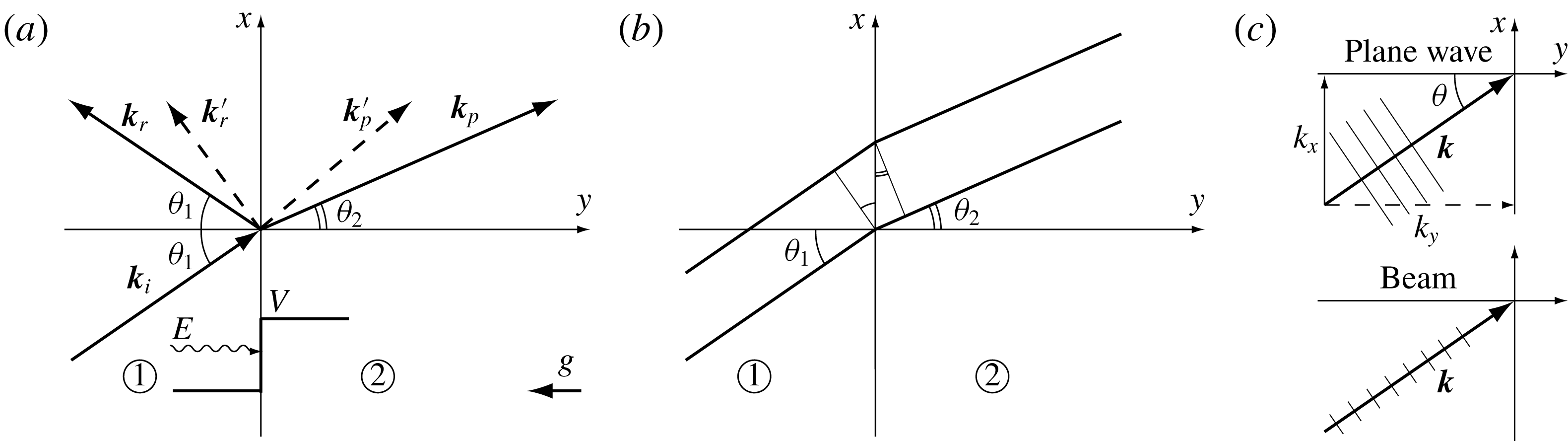
(a) Setting: incident (
 $i$
), reflected (
 $r$
) and refracted (
 $p$
) waves. (b) The change of an acoustic beam cross-section
 ${\mathcal{A}}$
:
 ${\mathcal{A}}_{i}/{\mathcal{A}}_{p}=\cos \unicode[STIX]{x1D703}_{1}/\cos \unicode[STIX]{x1D703}_{2}$
. (c) Two types of sound waves: plane and a narrow beam (a ray).

In the classical case of media with different densities
 $\unicode[STIX]{x1D70C}$
and sound speeds
 $c$
(cf. figure 1
a), the solutions to the wave equations in each medium for the velocity potential
 $\unicode[STIX]{x1D719}$
defined via
 $\unicode[STIX]{x1D735}\unicode[STIX]{x1D719}=\boldsymbol{v}$
,
 $$\begin{eqnarray}\unicode[STIX]{x1D719}_{tt}^{n}-c_{n}^{2}[\unicode[STIX]{x1D719}_{xx}^{n}+\unicode[STIX]{x1D719}_{yy}^{n}]=0,\quad \text{for}~x\in \mathbb{R},~y\in (-1)^{n}\mathbb{R}^{+},~n=1,2,\end{eqnarray}$$
satisfy the kinematic and dynamic conditions at the interface, linearized about its undisturbed position and with the notation
 $[\cdots ]_{1}^{2}$
for the jump of a quantity between two media represented as
 $$\begin{eqnarray}y=0:\quad [\unicode[STIX]{x1D719}_{y}]_{1}^{2}=0,\quad [p]_{1}^{2}=-[\unicode[STIX]{x1D70C}\unicode[STIX]{x1D719}_{t}]_{1}^{2}=0,\end{eqnarray}$$
accounting for the continuity (across the interface) of the vertical velocity component
 $v=\unicode[STIX]{x1D719}_{y}$
and the pressure
 $p$
, respectively. Representing the incident, reflected and transmitted waves as
 $\unicode[STIX]{x1D719}_{i}^{1}=A_{i}\text{e}^{\text{i}\unicode[STIX]{x1D713}_{i}}$
,
 $\unicode[STIX]{x1D719}_{r}^{1}=A_{r}\text{e}^{\text{i}\unicode[STIX]{x1D713}_{r}}$
and
 $\unicode[STIX]{x1D719}_{p}^{2}=A_{p}\text{e}^{\text{i}\unicode[STIX]{x1D713}_{p}}$
, correspondingly, with
 $\unicode[STIX]{x1D713}_{m}=\boldsymbol{k}_{m}\boldsymbol{\cdot }\boldsymbol{x}-\unicode[STIX]{x1D714}_{m}t$
(entailing that
 $\boldsymbol{v}\equiv (u,v)$
is parallel to
 $\boldsymbol{k}$
), where we have kept the frequencies
 $\unicode[STIX]{x1D714}_{m}$
and wavenumbers
 $\boldsymbol{k}_{m}=(k_{x}^{m},k_{y}^{m})$
independent, from (1.1) we find the corresponding dispersion relations:
 $$\begin{eqnarray}\unicode[STIX]{x1D714}_{i}^{2}=c_{1}^{2}|\boldsymbol{k}_{i}|^{2},\quad \unicode[STIX]{x1D714}_{r}^{2}=c_{1}^{2}|\boldsymbol{k}_{r}|^{2},\quad \unicode[STIX]{x1D714}_{p}^{2}=c_{2}^{2}|\boldsymbol{k}_{p}|^{2}.\end{eqnarray}$$
Substituting the velocity potentials into the boundary conditions (1.2) we conclude that the only way for the latter to hold is if
 $k_{x}^{i}=k_{x}^{r}=k_{x}^{p}\equiv k_{x}$
and
 $\unicode[STIX]{x1D714}_{i}=\unicode[STIX]{x1D714}_{r}=\unicode[STIX]{x1D714}_{p}\equiv \unicode[STIX]{x1D714}$
, i.e. the
 $x$
-component of the wavenumber remains unchanged and all three waves oscillate at the same frequency
 $\unicode[STIX]{x1D714}$
.
With these observations and the linear independence of the harmonics, equations (1.2) reduce to an algebraic system, i.e.
 $k_{y}^{i}A_{i}+k_{y}^{r}A_{r}=k_{y}^{p}A_{p}$
and
 $\unicode[STIX]{x1D70C}_{1}(A_{i}+A_{r})=\unicode[STIX]{x1D70C}_{2}A_{p}$
, the solution of which is
 $$\begin{eqnarray}\unicode[STIX]{x1D6E4}\equiv \frac{A_{r}}{A_{i}}=\frac{\unicode[STIX]{x1D70C}_{2}k_{y}-\unicode[STIX]{x1D70C}_{1}\unicode[STIX]{x1D705}_{y}}{\unicode[STIX]{x1D70C}_{2}k_{y}+\unicode[STIX]{x1D70C}_{1}\unicode[STIX]{x1D705}_{y}}\left(=\frac{\widehat{u}_{r}}{\widehat{u}_{i}}\right),\quad \frac{A_{p}}{A_{i}}=\frac{2\unicode[STIX]{x1D70C}_{1}k_{y}}{\unicode[STIX]{x1D70C}_{2}k_{y}+\unicode[STIX]{x1D70C}_{1}\unicode[STIX]{x1D705}_{y}}.\end{eqnarray}$$
Here the
 $y$
-components of
 $\boldsymbol{k}_{m}$
are determined from (1.3), i.e.
 $k_{y}^{m2}=\unicode[STIX]{x1D714}_{m}^{2}-k_{x}^{m2}$
and
 $$\begin{eqnarray}-k_{y}^{r}=k_{y}^{i}\equiv k_{y}=k_{x}/\tan \unicode[STIX]{x1D703}_{1},\quad k_{y}^{p}\equiv \unicode[STIX]{x1D705}_{y}=k_{x}/\tan \unicode[STIX]{x1D703}_{2},\end{eqnarray}$$
after we have used the above established facts that
 $k_{x}$
and
 $\unicode[STIX]{x1D714}$
are the same in both media. From the equality
 $k_{y}^{r}=-k_{y}^{i}$
it follows that the angle of incidence is equal to the angle of reflection,
 $\unicode[STIX]{x1D703}_{i}=\unicode[STIX]{x1D703}_{r}\equiv \unicode[STIX]{x1D703}_{1}$
, measured with respect to the normal to the boundary (cf. figure 1
a). With further geometric considerations we arrive at Snell’s (also known as Snell–Descartes’) law of refraction relating angles
 $\unicode[STIX]{x1D703}_{1}$
and
 $\unicode[STIX]{x1D703}_{2}$
:
 $$\begin{eqnarray}\frac{k_{x}^{i}}{k_{x}^{p}}=1=\frac{|\boldsymbol{k}_{i}|}{|\boldsymbol{k}_{p}|}\frac{\sin \unicode[STIX]{x1D703}_{1}}{\sin \unicode[STIX]{x1D703}_{2}}=\frac{\unicode[STIX]{x1D714}/c_{1}}{\unicode[STIX]{x1D714}/c_{2}}\frac{\sin \unicode[STIX]{x1D703}_{1}}{\sin \unicode[STIX]{x1D703}_{2}}\quad \Rightarrow \quad \frac{\sin \unicode[STIX]{x1D703}_{1}}{\sin \unicode[STIX]{x1D703}_{2}}=\frac{c_{1}}{c_{2}},\end{eqnarray}$$
with well-known properties (Kinsler et al.
Reference Kinsler, Frey, Coppens and Sanders1999). As follows from (1.4a), (1.5) and (1.6), for
 $\unicode[STIX]{x1D703}_{1}>\unicode[STIX]{x1D703}_{c}$
, where the critical angle
 $\unicode[STIX]{x1D703}_{c}$
is found from
 $\sin \unicode[STIX]{x1D703}_{1}=c_{1}/c_{2}$
for
 $c_{1}<c_{2}$
,
 $\unicode[STIX]{x1D705}_{y}$
becomes imaginary and hence the transmitted wave evanescent (though the transmitted wave energy is still non-zero), so that the Rayleigh reflection coefficient
 $\unicode[STIX]{x1D6E4}$
in (1.4a
) is no longer real. In fact,
 $\unicode[STIX]{x1D6E4}$
has complex conjugate numerator and denominator, meaning that its amplitude
 $|\unicode[STIX]{x1D6E4}|=1$
corresponds to total reflection, but since
 $\unicode[STIX]{x1D6E4}$
is complex there is a phase shift between the incident and reflected waves.
The energy conservation states that the averaged
 $\langle \,\cdot \,\rangle$
energy flux density
 $\boldsymbol{q}=p^{\prime }\boldsymbol{v}=\unicode[STIX]{x1D70C}c|\boldsymbol{v}|^{2}\boldsymbol{n}$
over the period
 $2\unicode[STIX]{x03C0}/\unicode[STIX]{x1D714}$
(here
 $\boldsymbol{n}=\boldsymbol{k}/k$
and
 $p^{\prime }$
is the pressure of the acoustic wave) in the reflected and transmitted waves should add up to that of the incident wave,
 $\langle {\mathcal{R}}_{0}\rangle +\langle {\mathcal{T}}_{0}\rangle =1$
, where the reflection and transmission coefficients are
 $\langle {\mathcal{R}}_{0}\rangle =\langle \boldsymbol{q}_{r}\boldsymbol{\cdot }\boldsymbol{n}_{r}\rangle /\langle \boldsymbol{q}_{i}\boldsymbol{\cdot }\boldsymbol{n}_{i}\rangle$
and
 $\langle {\mathcal{T}}_{0}\rangle =({\mathcal{A}}_{p}/{\mathcal{A}}_{i})\langle \boldsymbol{q}_{r}\boldsymbol{\cdot }\boldsymbol{n}_{r}\rangle /\langle \boldsymbol{q}_{i}\boldsymbol{\cdot }\boldsymbol{n}_{i}\rangle$
, respectively. Here we have taken into account the change in the beam cross-section between the transmitted
 ${\mathcal{A}}_{p}$
and incident
 ${\mathcal{A}}_{i}$
waves (with no change between incident and reflected waves); cf. figure 1(b). When
 $\unicode[STIX]{x1D703}_{1}>\unicode[STIX]{x1D703}_{c}$
,
 $\langle {\mathcal{R}}_{0}\rangle =1$
, but the instantaneous
 ${\mathcal{R}}_{0}$
is different from unity and, in fact, depends on
 $\unicode[STIX]{x1D714}$
. The sum of the instantaneous incident and reflected energy fluxes is non-zero, thus explaining the penetration of the acoustic signal into medium 2. The existence of the critical angle
 $\unicode[STIX]{x1D703}_{c}$
can be understood by rewriting (1.1) with
 $\unicode[STIX]{x1D719}^{n}(t,x,y)=\unicode[STIX]{x1D6F7}^{n}(y)\text{e}^{\text{i}(k_{x}x-\unicode[STIX]{x1D714}t)}$
, leading to the stationary one-dimensional (1D) Schrödinger equation
 $\unicode[STIX]{x1D6F7}_{yy}^{n}+(\unicode[STIX]{x1D714}^{2}/c_{n}^{2}-k_{x}^{2})\unicode[STIX]{x1D6F7}^{n}=0$
, where the expression in brackets has the meaning of the difference between the phonon energy
 $E$
and potential barrier size
 $V$
(cf. figure 1
a):
 $E-V\sim \unicode[STIX]{x1D714}^{2}/c_{n}^{2}-k_{x}^{2}$
with
 $V\sim \unicode[STIX]{x1D714}^{2}(1/c_{1}^{2}-1/c_{2}^{2})=[\unicode[STIX]{x1D714}^{2}/c^{2}]_{2}^{1}$
. For
 $c_{2}>c_{1}$
and
 $\unicode[STIX]{x1D703}_{1}>\unicode[STIX]{x1D703}_{c}$
, the energy of the incident phonon is below
 $V$
and hence it totally reflects from the interface.
2 Surface tension effects
Proceeding in the order of increasing complexity, we first account for surface (interfacial) tension
 $\unicode[STIX]{x1D70E}$
between two fluids. The wave equations (1.1) and hence the dispersion relation for sound propagation (1.3) stay intact as surface tension affects only the boundary conditions: (1.2a
) is appended with
 $h_{t}=\unicode[STIX]{x1D719}_{y}$
and (1.2b
) generalizes to
 $[\unicode[STIX]{x1D70C}\unicode[STIX]{x1D719}_{t}]_{1}^{2}=-\unicode[STIX]{x1D70E}h_{xx}$
. With the argument of § 1 and with an extra harmonic representation for the interfacial perturbation
 $h=A_{h}\text{e}^{\text{i}(k_{x}^{h}x-\unicode[STIX]{x1D714}_{h}t)}$
, we get three equations for unknown amplitudes
 $A_{r}$
,
 $A_{p}$
and
 $A_{h}$
with the resulting solutions:
 $$\begin{eqnarray}\{A_{r},A_{p},A_{h}\}/A_{i}=\unicode[STIX]{x1D6E5}^{-1}\{\unicode[STIX]{x1D70C}_{2}k_{y}-\unicode[STIX]{x1D70C}_{1}\unicode[STIX]{x1D705}_{y}+\text{i}\unicode[STIX]{x1D70E}k_{x}^{2}\unicode[STIX]{x1D705}_{y}k_{y}/\unicode[STIX]{x1D714}^{2},~2\unicode[STIX]{x1D70C}_{1}k_{y},~-2\unicode[STIX]{x1D70C}_{1}k_{y}\unicode[STIX]{x1D705}_{y}/\unicode[STIX]{x1D714}\},\end{eqnarray}$$
where
 $\unicode[STIX]{x1D6E5}=\unicode[STIX]{x1D70C}_{2}k_{y}+\unicode[STIX]{x1D70C}_{1}\unicode[STIX]{x1D705}_{y}+\text{i}\unicode[STIX]{x1D70E}k_{x}^{2}\unicode[STIX]{x1D705}_{y}k_{y}/\unicode[STIX]{x1D714}^{2}$
with the notation from (1.5). Notably, the amplitude of the interfacial wave
 $A_{h}$
does not vanish with
 $\unicode[STIX]{x1D70E}$
, which is due to the kinematic condition. The energy balance
 $\langle {\mathcal{R}}\rangle +\langle {\mathcal{T}}\rangle =1$
stays intact, i.e. in the steady state the surface waves do not withdraw energy from the incident wave due to the conservative nature of surface tension.
(a) Surface tension case:
 $\unicode[STIX]{x1D714}/\unicode[STIX]{x1D714}_{\unicode[STIX]{x1D70E}}^{(1)}=5$
. (b) Gravity case:
 $\unicode[STIX]{x1D714}/\unicode[STIX]{x1D714}_{g}^{(2)}=0.55$
. (c,d) Viscous cases:
 $\unicode[STIX]{x1D714}/\unicode[STIX]{x1D714}_{\unicode[STIX]{x1D708}}^{(2)}=1.0$
,
 $\unicode[STIX]{x1D70E}=0$
, with
 $\unicode[STIX]{x1D707}_{1}/\unicode[STIX]{x1D707}_{2}=0.5$
(c) and 3.5 (d). In all plots
 $c_{1}/c_{2}=1.5$
and
 $\unicode[STIX]{x1D70C}_{1}/\unicode[STIX]{x1D70C}_{2}=1.25$
. Ticks and lower/upper limits of the ordinate are the same in (a–d). Solid lines correspond to
 $\langle {\mathcal{R}}\rangle$
and dashed to
 $\langle {\mathcal{T}}\rangle$
, while thin ones to the classical
 $\langle {\mathcal{R}}_{0}\rangle$
and
 $\langle {\mathcal{T}}_{0}\rangle$
.

The complexity of the amplitudes, in particular
 $A_{r}$
, implies that there is a phase
 $\unicode[STIX]{x1D711}$
associated with it so that the corresponding reflected wave behaves as
 $\unicode[STIX]{x1D719}_{r}^{1}\sim \text{e}^{\text{i}(\unicode[STIX]{x1D713}_{r}+\unicode[STIX]{x1D711})}$
, i.e. the phase constant
 $\unicode[STIX]{x1D711}$
tells us how much a signal is shifted in time and how efficiently energy is transferred from the driver (incident wave) to the oscillator system (reflected wave). Exploiting a simple relation between time averaging and multiplication of complex amplitudes,
 $$\begin{eqnarray}\langle (A\text{e}^{+}+A^{\ast }\text{e}^{-})(B\text{e}^{+}+B^{\ast }\text{e}^{-})\rangle =2(A_{\text{r}}B_{\text{r}}+A_{\text{i}}B_{\text{i}}),\end{eqnarray}$$
e.g. when
 $B\equiv A$
,
 $\langle (A\text{e}^{+}+A^{\ast }\text{e}^{-})^{2}\rangle =2|A|^{2}$
, in the case of regular reflection,
 $\unicode[STIX]{x1D703}_{1}<\unicode[STIX]{x1D703}_{c}$
, we find
 $$\begin{eqnarray}\hspace{-8.0pt}\langle {\mathcal{R}}\rangle =\frac{(k_{y}\unicode[STIX]{x1D70C}_{2}-\unicode[STIX]{x1D705}_{y}\unicode[STIX]{x1D70C}_{1})^{2}+\unicode[STIX]{x1D70E}^{2}k_{y}^{2}\unicode[STIX]{x1D705}_{y}^{2}k_{x}^{4}/\unicode[STIX]{x1D714}^{4}}{(k_{y}\unicode[STIX]{x1D70C}_{2}+\unicode[STIX]{x1D705}_{y}\unicode[STIX]{x1D70C}_{1})^{2}+\unicode[STIX]{x1D70E}^{2}k_{y}^{2}\unicode[STIX]{x1D705}_{y}^{2}k_{x}^{4}/\unicode[STIX]{x1D714}^{4}},\quad \tan \unicode[STIX]{x1D711}=\frac{2\unicode[STIX]{x1D70E}\unicode[STIX]{x1D70C}_{1}k_{y}\unicode[STIX]{x1D705}_{y}^{2}k_{x}^{2}/\unicode[STIX]{x1D714}^{2}}{k_{y}^{2}\unicode[STIX]{x1D70C}_{2}^{2}-\unicode[STIX]{x1D705}_{y}^{2}\unicode[STIX]{x1D70C}_{1}^{2}+\unicode[STIX]{x1D70E}^{2}k_{y}^{2}\unicode[STIX]{x1D705}_{y}^{2}k_{x}^{4}/\unicode[STIX]{x1D714}^{4}},\end{eqnarray}$$
where
 $\unicode[STIX]{x1D711}=\arg \unicode[STIX]{x1D6E4}$
. The latter expression (for
 $\unicode[STIX]{x1D711}$
) suggests that surface tension can be responsible for both leading and lagging effects depending on the sign of the denominator in the argument of
 $\tan ^{-1}$
. As follows from (2.3), the reflection phenomena are characterized by three non-dimensional parameters, i.e.
 $\unicode[STIX]{x1D70C}_{1}/\unicode[STIX]{x1D70C}_{2}$
,
 $c_{1}/c_{2}$
and
 $\unicode[STIX]{x1D714}/\unicode[STIX]{x1D714}_{\unicode[STIX]{x1D70E}}^{(1)}$
with
 $\unicode[STIX]{x1D714}_{\unicode[STIX]{x1D70E}}^{(1)}=c_{1}^{3}\unicode[STIX]{x1D70C}_{1}/\unicode[STIX]{x1D70E}$
evaluated in medium 1, and for particular values are illustrated in figure 2(a) exhibiting significant departures from the classical case when
 $\unicode[STIX]{x1D714}\sim \unicode[STIX]{x1D714}_{\unicode[STIX]{x1D70E}}$
. The value of
 $\langle {\mathcal{R}}\rangle$
is closer to unity than that of
 $\langle {\mathcal{R}}_{0}\rangle$
and, in fact, the reflection becomes stronger with increasing frequency
 $\unicode[STIX]{x1D714}$
, meaning that surface tension ‘rigidifies’ the interface, leading to enhanced reflection. While, as is obvious from (2.3), perfect refraction is no longer possible in the presence of surface tension, one can still find a minimum of reflection
 $$\begin{eqnarray}\langle {\mathcal{R}}\rangle _{min}=\frac{\unicode[STIX]{x1D70E}^{2}(c_{1}^{2}-c_{2}^{2})k_{x}^{6}}{\unicode[STIX]{x1D70E}^{2}k_{x}^{4}(c_{1}^{2}-c_{2}^{2})-4\unicode[STIX]{x1D714}^{4}(c_{1}^{2}\unicode[STIX]{x1D70C}_{1}^{2}-c_{2}^{2}\unicode[STIX]{x1D70C}_{2}^{2})},\end{eqnarray}$$
which occurs at the classical Brewster angle
 $\sin ^{2}\unicode[STIX]{x1D703}_{B}=[1-(\unicode[STIX]{x1D70C}_{1}c_{1}/\unicode[STIX]{x1D70C}_{2}c_{2})^{2}]/[1-(\unicode[STIX]{x1D70C}_{1}/\unicode[STIX]{x1D70C}_{2})^{2}]$
. In the case of total reflection, i.e. when
 $\unicode[STIX]{x1D703}_{1}>\unicode[STIX]{x1D703}_{c}$
with
 $\sin \unicode[STIX]{x1D703}_{c}=c_{1}/c_{2}$
, the averaging gives
 $\langle {\mathcal{R}}\rangle =1$
.
3 Gravity effects
Starting from the Euler system for compressible flow in the gravity field
 $\boldsymbol{g}$
and superimposing small perturbations of density
 $\unicode[STIX]{x1D70C}^{\prime }$
and pressure
 $p^{\prime }$
on the hydrostatic base state
 $(\unicode[STIX]{x1D70C}_{0},p_{0})$
governed by
 $p_{0}=\int \unicode[STIX]{x1D70C}_{0}\,\boldsymbol{g}\boldsymbol{\cdot }\text{d}\boldsymbol{x}$
, the linearized system for perturbation reads
 $$\begin{eqnarray}\frac{\unicode[STIX]{x2202}\unicode[STIX]{x1D70C}^{\prime }}{\unicode[STIX]{x2202}t}+\unicode[STIX]{x1D70C}_{0}\unicode[STIX]{x1D735}\boldsymbol{\cdot }\boldsymbol{v}+\unicode[STIX]{x1D735}\unicode[STIX]{x1D70C}_{0}\boldsymbol{\cdot }\boldsymbol{v}=0,\quad \frac{\unicode[STIX]{x2202}\boldsymbol{v}}{\unicode[STIX]{x2202}t}=-\frac{1}{\unicode[STIX]{x1D70C}_{0}}\unicode[STIX]{x1D735}p^{\prime }+\boldsymbol{g}\frac{\unicode[STIX]{x1D70C}^{\prime }}{\unicode[STIX]{x1D70C}_{0}},\end{eqnarray}$$
where the last term in (3.1a
) comes from the base state density stratification and the last term in (3.1b
) has the meaning of buoyancy. The perturbation for pressure
 $p^{\prime }$
is found from
 $$\begin{eqnarray}p=p_{0}+p^{\prime }=p_{0}+(\unicode[STIX]{x2202}p/\unicode[STIX]{x2202}\unicode[STIX]{x1D70C})_{s,\unicode[STIX]{x1D70C}_{0}}\unicode[STIX]{x1D70C}^{\prime }+\cdots \quad \Rightarrow \quad p^{\prime }=(\unicode[STIX]{x2202}p/\unicode[STIX]{x2202}\unicode[STIX]{x1D70C})_{s,\unicode[STIX]{x1D70C}_{0}}\unicode[STIX]{x1D70C}^{\prime }=c_{0}^{2}\unicode[STIX]{x1D70C}^{\prime },\end{eqnarray}$$
after using the adiabatic assumption (constant entropy
 $s$
) for sound wave propagation, to be revisited in § 4. The corresponding interfacial conditions are again the kinematic and dynamic
 $$\begin{eqnarray}y=0:\quad h_{t}=v^{1}=v^{2},\quad [p^{\prime }]_{1}^{2}=[c_{0}^{2}\unicode[STIX]{x1D70C}^{\prime }]_{1}^{2}=\unicode[STIX]{x1D70E}h_{xx}\quad \Rightarrow \quad [c_{0}^{2}\unicode[STIX]{x1D70C}_{t}^{\prime }]_{1}^{2}=\unicode[STIX]{x1D70E}h_{txx},\end{eqnarray}$$
where in the latter condition we exploited (3.2) and differentiated with respect to time as our goal is a closed system for velocity only. The time derivative of density is found from the continuity equation (3.1a
). In what follows we will consider the case when gravitational acceleration is directed along the negative
 $y$
-axis,
 $\boldsymbol{g}=(0,-g)$
with
 $g>0$
as per figure 1(a).
Eliminating
 $\unicode[STIX]{x1D70C}^{\prime }$
from (3.1), we get a vector wave-like equation for the velocity field:
 $$\begin{eqnarray}\frac{\unicode[STIX]{x2202}^{2}\boldsymbol{v}}{\unicode[STIX]{x2202}t^{2}}=\frac{c_{0}^{2}}{\unicode[STIX]{x1D70C}_{0}}[(\unicode[STIX]{x1D735}\unicode[STIX]{x1D70C}_{0}+\unicode[STIX]{x1D70C}_{0}\unicode[STIX]{x1D735})\unicode[STIX]{x1D735}\boldsymbol{\cdot }\boldsymbol{v}+\unicode[STIX]{x1D735}(\unicode[STIX]{x1D735}\unicode[STIX]{x1D70C}_{0}\boldsymbol{\cdot }\boldsymbol{v})]-\widetilde{\boldsymbol{g}}\left[\unicode[STIX]{x1D735}\boldsymbol{\cdot }\boldsymbol{v}+\frac{1}{\unicode[STIX]{x1D70C}_{0}}\unicode[STIX]{x1D735}\unicode[STIX]{x1D70C}_{0}\boldsymbol{\cdot }\boldsymbol{v}\right],\end{eqnarray}$$
where
 $\widetilde{\boldsymbol{g}}=\boldsymbol{g}-(\text{d}^{2}p_{0}/\text{d}\unicode[STIX]{x1D70C}_{0}^{2})\unicode[STIX]{x1D735}\unicode[STIX]{x1D70C}_{0}$
, and the term
 $\unicode[STIX]{x1D735}(\unicode[STIX]{x1D735}\unicode[STIX]{x1D70C}_{0}\boldsymbol{\cdot }\boldsymbol{v})$
clearly contains vorticity
 $\unicode[STIX]{x1D74E}=\unicode[STIX]{x1D735}\times \boldsymbol{v}$
, which means that in the presence of stratification the flow is in general no longer irrotational. Equation (3.4) illustrates how gravity enters under two guises: (i) pure gravity effect in the term
 $\boldsymbol{g}\unicode[STIX]{x1D735}\boldsymbol{\cdot }\boldsymbol{v}$
, and (ii) through explicit density stratification, i.e. the terms involving
 $\unicode[STIX]{x1D735}\unicode[STIX]{x1D70C}_{0}$
. Depending on the physical situation, one of these two effects is dominant. Since we are interested in the interaction of sound waves with the horizontal interface rather than propagation through media, which has been studied before (Tolstoy Reference Tolstoy1963, Reference Tolstoy1965), for transparency we will first elaborate on the case (i) when the explicit base state density stratification can be neglected,
 $\unicode[STIX]{x1D735}\unicode[STIX]{x1D70C}_{0}\simeq 0$
, and also assume
 $\unicode[STIX]{x1D70C}_{0}(\text{d}^{2}p_{0}/\text{d}\unicode[STIX]{x1D70C}_{0}^{2})/(\text{d}p_{0}/\text{d}\unicode[STIX]{x1D70C}_{0})\ll 1$
, which allows us to neglect the variation of the sound speed
 $c_{0}$
with altitude
 $y$
, for example, in the case of an ideal gas under isothermal conditions. The condition
 $\unicode[STIX]{x1D735}\unicode[STIX]{x1D70C}_{0}\simeq 0$
is equivalent to assuming that
 $\unicode[STIX]{x1D714}_{g}$
is disparate from (either much smaller or much larger than)
 $\unicode[STIX]{x1D714}_{g}^{\prime }$
. Then (3.4) for velocity
 $\boldsymbol{v}$
and the corresponding equation for density variation
 $\unicode[STIX]{x1D70C}^{\prime }$
reduce to
 $$\begin{eqnarray}\frac{\unicode[STIX]{x2202}^{2}\boldsymbol{v}}{\unicode[STIX]{x2202}t^{2}}=c_{0}^{2}\unicode[STIX]{x1D735}(\unicode[STIX]{x1D735}\boldsymbol{\cdot }\boldsymbol{v})-\boldsymbol{g}\unicode[STIX]{x1D735}\boldsymbol{\cdot }\boldsymbol{v},\quad \frac{\unicode[STIX]{x2202}^{2}\unicode[STIX]{x1D70C}^{\prime }}{\unicode[STIX]{x2202}t^{2}}=c_{0}^{2}\unicode[STIX]{x1D6FB}^{2}\unicode[STIX]{x1D70C}^{\prime }-\boldsymbol{g}\boldsymbol{\cdot }\unicode[STIX]{x1D735}\unicode[STIX]{x1D70C}^{\prime }.\end{eqnarray}$$
Plugging the solution of the form
 $(uv)^{\text{T}}=(\widehat{u}\,\widehat{v})^{\text{T}}\text{e}^{\text{i}\unicode[STIX]{x1D713}}$
in (3.5a
) leads to the dispersion relation
 $$\begin{eqnarray}\unicode[STIX]{x1D714}^{4}-[(\boldsymbol{k}\boldsymbol{\cdot }\boldsymbol{k})c_{0}^{2}-\text{i}gk_{y}]\unicode[STIX]{x1D714}^{2}=0,\end{eqnarray}$$
where we have used the notation
 $\boldsymbol{k}\boldsymbol{\cdot }\boldsymbol{k}$
to differentiate from
 $|\boldsymbol{k}|^{2}$
as the wavenumber vector
 $\boldsymbol{k}$
is now complex as opposed to the classical case (§ 1). The dispersion relation (3.6) is the deep water limit of that for acoustic gravity waves with a free surface (Dalrymple & Rogers Reference Dalrymple, Rogers and Smith2007; Kadri & Stiassnie Reference Kadri and Stiassnie2013). Equation (3.6) yields two solutions: the travelling
 $\unicode[STIX]{x1D714}_{1}^{2}=(\boldsymbol{k}\boldsymbol{\cdot }\boldsymbol{k})c_{0}^{2}-\text{i}gk_{y}$
and standing
 $\unicode[STIX]{x1D714}_{2}^{2}=0$
waves, which apply in every medium with an appropriate speed of sound. The corresponding eigenvectors provide a relation between the velocity components:
 $$\begin{eqnarray}\unicode[STIX]{x1D714}_{1}:\quad \widehat{v}=\widehat{u}(k_{y}-\text{i}g/c_{0}^{2})/k_{x},\quad \unicode[STIX]{x1D714}_{2}:\quad \widehat{v}=-\widehat{u}k_{x}/k_{y},\end{eqnarray}$$
i.e. the former is akin to the usual potential flow solution and the latter is a vorticity mode with the velocity vector
 $\boldsymbol{v}$
no longer parallel to that of the wavenumber
 $\boldsymbol{k}$
.
Given that these modes are decoupled and we are interested in sound waves of non-vanishing frequency, we will focus on the ‘potential flow’ case (though a velocity potential as such does not exist). The dispersion relation (3.6) requires further interpretation since the wavenumber
 $\boldsymbol{k}$
is always complex as opposed to the classical case (§ 1). As follows from (3.6), if the
 $y$
-component of the wavenumber is zero, then we arrive at the classical acoustic dispersion (1.3), i.e.
 $k_{x}c_{0}=\unicode[STIX]{x1D714}$
. This means that the gravity vector introduces an anisotropy: when
 $\boldsymbol{k}=(k_{x},0)$
, gravity does not have any effect on the sound wave (in the same way as gravity does not change the horizontal velocity of a thrown stone), while for
 $\boldsymbol{k}=(0,k_{y})$
the wavenumber becomes complex, with the imaginary part being responsible for decay/growth of the sound wave amplitude. In general, the direction of a plane sound wave, even in the presence of decay in a certain direction, is determined by the real part of the wavenumber vector, so that in our case
 $k_{x}\equiv k_{x}^{\text{r}}=k\sin \unicode[STIX]{x1D703}$
and
 $k_{y}^{\text{r}}=k\cos \unicode[STIX]{x1D703}$
are real, while
 $k_{y}=k_{y}^{\text{r}}+\text{i}k_{y}^{\text{i}}$
. Since
 $\boldsymbol{k}\boldsymbol{\cdot }\boldsymbol{k}=k_{x}^{2}+k_{y}^{2}$
, then (3.6) yields
 $$\begin{eqnarray}k_{x}=k\sin \unicode[STIX]{x1D703},\quad k_{y}=\frac{\text{i}g\pm \sqrt{-g^{2}+4c_{0}^{2}(\unicode[STIX]{x1D714}^{2}-k_{x}^{2}c_{0}^{2})}}{2c_{0}^{2}},\quad \text{where}~k^{2}=\frac{\unicode[STIX]{x1D714}^{2}}{c_{0}^{2}}-\frac{g^{2}}{4c_{0}^{4}}.\quad\end{eqnarray}$$
Note that
 $k^{2}\neq |\boldsymbol{k}|^{2}$
. An important conclusion from the above formula for
 $k_{y}$
and (3.7a
) is that the
 $x$
-component of the velocity experiences a jump across the interface since
 $k_{x}$
is the same for all waves in both media, but the vertical velocity component is continuous based on (3.3a
). Given the continuity of the
 $x$
-component of the wavenumber, we derive a modified Snell’s law:
 $$\begin{eqnarray}\frac{k_{x}^{i}}{k_{x}^{p}}=1=\frac{k_{i}}{k_{p}}\frac{\sin \unicode[STIX]{x1D703}_{1}}{\sin \unicode[STIX]{x1D703}_{2}}=\frac{\sqrt{\unicode[STIX]{x1D714}^{2}/c_{1}^{2}-g^{2}/4c_{1}^{4}}}{\sqrt{\unicode[STIX]{x1D714}^{2}/c_{2}^{2}-g^{2}/4c_{2}^{4}}}\frac{\sin \unicode[STIX]{x1D703}_{1}}{\sin \unicode[STIX]{x1D703}_{2}}\hspace{8.00003pt}\Rightarrow \hspace{8.00003pt}\frac{\sin \unicode[STIX]{x1D703}_{1}}{\sin \unicode[STIX]{x1D703}_{2}}=\frac{c_{1}}{c_{2}}\frac{\sqrt{\unicode[STIX]{x1D714}^{2}-g^{2}/4c_{2}^{2}}}{\sqrt{\unicode[STIX]{x1D714}^{2}-g^{2}/4c_{1}^{2}}},\quad\end{eqnarray}$$
which recovers the classical one (1.6) in the limit
 $g\rightarrow 0$
. The case of pure gravity effect without surface tension leads to a concise expression for the Rayleigh reflection coefficient:
 $$\begin{eqnarray}\frac{\widehat{u}_{r}}{\widehat{u}_{i}}=\frac{(g^{2}+4c_{2}^{4}k_{2}^{2})(\text{i}g-2c_{1}^{2}k_{1}\cos \unicode[STIX]{x1D703}_{1})\unicode[STIX]{x1D70C}_{2}-(g^{2}+4c_{1}^{4}k_{1}^{2})(\text{i}g-2c_{2}^{2}k_{2}\cos \unicode[STIX]{x1D703}_{2})\unicode[STIX]{x1D70C}_{1}}{(g^{2}+4c_{1}^{4}k_{1}^{2})(\text{i}g-2c_{2}^{2}k_{2}\cos \unicode[STIX]{x1D703}_{2})\unicode[STIX]{x1D70C}_{1}-(g^{2}+4c_{2}^{4}k_{2}^{2})(\text{i}g+2c_{1}^{2}k_{1}\cos \unicode[STIX]{x1D703}_{1})\unicode[STIX]{x1D70C}_{2}},\end{eqnarray}$$
where
 $k_{1,2}$
are given by (3.8) for the corresponding medium, and the angle
 $\unicode[STIX]{x1D703}_{2}$
is found from (3.9).
Let us consider energy balance in the case treated here, i.e. when the explicit gradient of the base state density can be neglected in (3.1). Taking the scalar product of the velocity vector
 $\boldsymbol{v}$
with the momentum equation (3.1b
) and using (3.2), we find
 $$\begin{eqnarray}\frac{\unicode[STIX]{x2202}}{\unicode[STIX]{x2202}t}\left[\frac{1}{2}\unicode[STIX]{x1D70C}_{0}\boldsymbol{v}\boldsymbol{\cdot }\boldsymbol{v}+\frac{1}{2}\frac{p^{\prime 2}}{\unicode[STIX]{x1D70C}_{0}c_{0}^{2}}\right]=-\unicode[STIX]{x1D735}\boldsymbol{\cdot }(p^{\prime }\boldsymbol{v})+\boldsymbol{v}\boldsymbol{\cdot }\boldsymbol{g}\frac{p^{\prime }}{c_{0}^{2}},\end{eqnarray}$$
which shows the dynamic energy balance for a sound wave in some control volume
 $D$
. The expression on the left is the sum of kinetic and potential compression energies, while the first term on the right is the energy flux
 $\boldsymbol{q}=p^{\prime }\boldsymbol{v}$
through the boundary
 $\unicode[STIX]{x2202}D$
and the second term is the production of energy inside the volume
 $D$
by the gravity force. Hence, the energy density flux is the same as in the classical case, though the expression for
 $p^{\prime }$
is different with the amplitude
 $\widehat{p}=\widehat{u}\unicode[STIX]{x1D714}\unicode[STIX]{x1D70C}_{0}/k_{x}$
. The behaviour of the reflection
 $\langle {\mathcal{R}}\rangle$
and transmission
 $\langle {\mathcal{T}}\rangle$
coefficients corresponding to (3.10) for averaged energy fluxes calculated with (2.2) is illustrated in figure 2(b) showing a significant shift in total reflection compared to the classical case if
 $\unicode[STIX]{x1D714}\sim \unicode[STIX]{x1D714}_{g}$
in accordance with (3.9), the physics of which is explained below. As we can also see from figure 2(b), the reflection coefficient increases and thus the transmission coefficient decreases due to the pure gravity effect, which should be contrasted to the recent observation (Godin Reference Godin2006; Godin & Fuks Reference Godin and Fuks2012) of increased sound transmission from a point source if it is located close to the interface within a fraction of the wavelength and the base state density variation is taken into account. A possibility of an analogous behaviour in the context of the present analysis will be pointed out below when the case of density stratification is addressed.
To proceed with the energy considerations, note that the wave equation for the density variation (3.5b
) is clearly not self-adjoint, thus having implications for energy balance. With the change of variable
 $\unicode[STIX]{x1D70C}^{\prime }=\text{e}^{-\widehat{\boldsymbol{g}}\boldsymbol{\cdot }\boldsymbol{x}/2}\widetilde{\unicode[STIX]{x1D70C}}^{\prime }$
, where
 $\widehat{\boldsymbol{g}}=-\boldsymbol{g}/c_{0}^{2}$
, (3.5b
) reduces to a self-adjoint Klein–Gordon equation for particles with a non-zero mass (Fermi Reference Fermi1951):
 $\unicode[STIX]{x2202}^{2}\widetilde{\unicode[STIX]{x1D70C}}^{\prime }/\unicode[STIX]{x2202}t^{2}=c_{0}^{2}\unicode[STIX]{x1D6FB}^{2}\widetilde{\unicode[STIX]{x1D70C}}^{\prime }-\widetilde{\unicode[STIX]{x1D70C}}^{\prime }|\boldsymbol{g}|^{2}/4c_{0}^{2}$
, as opposed to the massless D’Alembert equation (1.1). Letting
 $\widetilde{\unicode[STIX]{x1D70C}}^{\prime }\sim \text{e}^{\text{i}(\boldsymbol{k}\boldsymbol{\cdot }\boldsymbol{x}-\unicode[STIX]{x1D714}t)}$
, we recover the gravity-modified dispersion relation (3.8). Also, following the analysis of § 1, with
 $\widetilde{\unicode[STIX]{x1D70C}}^{\prime }=\widehat{\unicode[STIX]{x1D70C}}^{\prime }(y)\text{e}^{\text{i}(k_{x}x-\unicode[STIX]{x1D714}t)}$
we get another stationary 1D Schrödinger equation
 $\widehat{\unicode[STIX]{x1D70C}}_{yy}^{\prime }+(\unicode[STIX]{x1D714}^{2}/c^{2}-k_{x}^{2}-g^{2}/4c_{0}^{4})\widehat{\unicode[STIX]{x1D70C}}^{\prime }=0$
, from which it follows that the potential barrier size
 $$\begin{eqnarray}V\sim [\unicode[STIX]{x1D714}^{2}/c^{2}-g^{2}/4c^{4}]_{2}^{1}\end{eqnarray}$$
differs from the classical case (§ 1), affecting not only the total reflection angle
 $\unicode[STIX]{x1D703}_{c}$
, but also the reflection/transmission even when the phonon energy
 $E>V$
. Owing to the conservative nature of gravity, the total energy balance is still the same,
 $\langle {\mathcal{R}}\rangle +\langle {\mathcal{T}}\rangle =1$
. The mass-like effect of gravity explains the increased reflection in figure 2(b) for the configuration shown in figure 1(a).
It is important to remark that, in the presence of stratification,
 $\unicode[STIX]{x1D735}\unicode[STIX]{x1D70C}_{0}\neq 0$
, but when the sound speed variation is neglected, (3.4) admits the potential flow (
 $\boldsymbol{v}=\unicode[STIX]{x1D735}\unicode[STIX]{x1D719}$
) formulation (Bondi Reference Bondi1947; Abdolali & Kirby Reference Abdolali and Kirby2017)
 $$\begin{eqnarray}\frac{\unicode[STIX]{x2202}^{2}\unicode[STIX]{x1D719}}{\unicode[STIX]{x2202}t^{2}}=c_{0}^{2}\unicode[STIX]{x1D6FB}^{2}\unicode[STIX]{x1D719}+g\frac{\unicode[STIX]{x2202}\unicode[STIX]{x1D719}}{\unicode[STIX]{x2202}y},\end{eqnarray}$$
which leads to exactly the same travelling wave solution as the dispersion relation (3.6) in the above considered case (i) of the pure gravity effect and hence the same modified Snell’s law (3.9).
In the general case, however, when both density stratification and sound speed variation are taken into account (3.4), the initially plane wave neither stays plane nor preserves its direction due to refraction (Brekhovskikh Reference Brekhovskikh1960), which can be easily seen if one approximates the continuous stratification by discrete layers with different sound speeds and then applies (3.9). Hence, in this case the universality of a Snell’s type law is lost – the angle of incidence at a particular point of the interface depends not only on the initial direction of the plane wave, but also on the distance travelled and the particularities of the sound speed variation. Nevertheless, the dispersion relation corresponding to (3.4) provides leading-order corrections (expanded here for small
 $\dot{\unicode[STIX]{x1D70C}}_{0}$
,
 $\ddot{\unicode[STIX]{x1D70C}}_{0}$
and
 $g$
assuming slow variation of
 $\unicode[STIX]{x1D70C}_{0}$
with
 $y$
, so that
 $\unicode[STIX]{x1D714}_{1,2}$
and
 $k_{y}$
are slow functions of
 $y$
as well) to the frequencies
 $\unicode[STIX]{x1D714}_{1,2}$
determined above:
 $$\begin{eqnarray}\unicode[STIX]{x1D714}_{1}^{2}=(\boldsymbol{k}\boldsymbol{\cdot }\boldsymbol{k})c_{0}^{2}-\text{i}\widetilde{g}k_{y}-2\text{i}k_{y}c_{0}^{2}\frac{\dot{\unicode[STIX]{x1D70C}}_{0}}{\unicode[STIX]{x1D70C}_{0}}-\frac{c_{0}^{2}k_{y}^{2}}{(\boldsymbol{k}\boldsymbol{\cdot }\boldsymbol{k})}\frac{\ddot{\unicode[STIX]{x1D70C}}_{0}}{\unicode[STIX]{x1D70C}_{0}},\quad \unicode[STIX]{x1D714}_{2}^{2}=-\frac{c_{0}^{2}k_{x}^{2}}{(\boldsymbol{k}\boldsymbol{\cdot }\boldsymbol{k})}\frac{\ddot{\unicode[STIX]{x1D70C}}_{0}}{\unicode[STIX]{x1D70C}_{0}},\end{eqnarray}$$
where
 $k_{y}$
is general, not undisturbed wavenumber component, and
 $\widetilde{g}=g-(\text{d}^{2}p_{0}/\text{d}\unicode[STIX]{x1D70C}_{0}^{2})\dot{\unicode[STIX]{x1D70C}}_{0}$
. Thus, the standing wave solution for
 $\unicode[STIX]{x1D735}\unicode[STIX]{x1D70C}_{0}\simeq 0$
is no longer standing for
 $\unicode[STIX]{x1D735}\unicode[STIX]{x1D70C}_{0}\neq 0$
, with the corresponding eigenvectors again accounting for the potential and vorticity modes:
 $$\begin{eqnarray}\displaystyle & \displaystyle \unicode[STIX]{x1D714}_{1}:\quad \widehat{v}=\widehat{u}\frac{k_{y}}{k_{x}}\left(1-\frac{\unicode[STIX]{x1D6FE}}{k_{y}}-\text{i}\frac{\widetilde{g}}{c_{0}^{2}k_{y}}\right), & \displaystyle\end{eqnarray}$$
 $$\begin{eqnarray}\displaystyle & \displaystyle \unicode[STIX]{x1D714}_{2}:\quad \widehat{v}=-\widehat{u}\frac{k_{x}}{k_{y}}\left(1+\frac{\unicode[STIX]{x1D6FE}}{k_{y}}\right),\quad \text{where}~\unicode[STIX]{x1D6FE}=\text{i}\frac{\dot{\unicode[STIX]{x1D70C}}_{0}}{\unicode[STIX]{x1D70C}_{0}}+\frac{k_{y}}{(\boldsymbol{k}\boldsymbol{\cdot }\boldsymbol{k})}\frac{\ddot{\unicode[STIX]{x1D70C}}_{0}}{\unicode[STIX]{x1D70C}_{0}}. & \displaystyle\end{eqnarray}$$
 $x$
-component of the wavenumber
 $\boldsymbol{k}$
is real and given upon arrival at the interface, from (3.14a
) we can find the
 $y$
-component of the corresponding wavenumber expanded here for both small base state density variations and gravity:
 $$\begin{eqnarray}k_{y}=k_{0y}\left(\pm 1-\frac{c_{0}^{2}}{2\unicode[STIX]{x1D714}^{2}}\frac{\ddot{\unicode[STIX]{x1D70C}}_{0}}{\unicode[STIX]{x1D70C}_{0}}\right)+\text{i}\frac{\dot{\unicode[STIX]{x1D70C}}_{0}}{\unicode[STIX]{x1D70C}_{0}}+\text{i}\frac{g}{2c_{0}^{2}}+O(g^{2}),\quad k_{0y}=\sqrt{(\unicode[STIX]{x1D714}/c_{0})^{2}-k_{x}^{2}},\end{eqnarray}$$
where
 $k_{0y}$
is the undisturbed
 $y$
-component of the wavenumber in the absence of gravity (1.5). Given the relation between
 $\widehat{u}$
and
 $\widehat{v}$
, we can solve (3.3) perturbatively for the amplitudes of the reflected and refracted waves in the presence of surface tension, e.g. the correction
 $\unicode[STIX]{x1D6FF}\widehat{u}_{r}$
to
 $\widehat{u}_{r}$
given by (2.1), so that the total solution is
 $\widehat{u}_{r}+\unicode[STIX]{x1D6FF}\widehat{u}_{r}$
, with the singled out effect of density stratification reads
 $$\begin{eqnarray}\frac{\unicode[STIX]{x1D6FF}\widehat{u}_{r}}{\widehat{u}_{i}}=-k_{y}\unicode[STIX]{x1D705}_{y}\unicode[STIX]{x1D714}^{2}\frac{(\unicode[STIX]{x1D73F}\boldsymbol{\cdot }\unicode[STIX]{x1D73F})(\text{i}k_{x}\unicode[STIX]{x1D705}_{y}\unicode[STIX]{x1D70E}+\unicode[STIX]{x1D714}^{2}\unicode[STIX]{x1D70C}_{2})\ddot{\unicode[STIX]{x1D70C}}_{1}-(\boldsymbol{k}\boldsymbol{\cdot }\boldsymbol{k})\unicode[STIX]{x1D714}^{2}\unicode[STIX]{x1D70C}_{1}\ddot{\unicode[STIX]{x1D70C}}_{2}}{(\boldsymbol{k}\boldsymbol{\cdot }\boldsymbol{k})(\unicode[STIX]{x1D73F}\boldsymbol{\cdot }\unicode[STIX]{x1D73F})[\unicode[STIX]{x1D705}_{y}(\text{i}k_{x}^{2}k_{y}\unicode[STIX]{x1D70E}+\unicode[STIX]{x1D714}^{2}\unicode[STIX]{x1D70C}_{1})+k_{y}\unicode[STIX]{x1D714}^{2}\unicode[STIX]{x1D70C}_{2}]^{2}},\end{eqnarray}$$
which is real-valued for
 $\unicode[STIX]{x1D70E}=0$
, and with the pure gravity effect (no explicit stratification) reads
 $$\begin{eqnarray}\frac{\unicode[STIX]{x1D6FF}\widehat{u}_{r}}{\widehat{u}_{i}}=k_{y}\unicode[STIX]{x1D70C}_{1}\frac{\unicode[STIX]{x1D70E}[k_{x}^{4}\unicode[STIX]{x1D705}_{y}-(\boldsymbol{k}\boldsymbol{\cdot }\boldsymbol{k})k_{x}^{2}\unicode[STIX]{x1D705}_{y}+k_{x}^{2}k_{y}\unicode[STIX]{x1D705}_{y}^{2}]-\text{i}\unicode[STIX]{x1D714}^{2}[(\unicode[STIX]{x1D73F}\boldsymbol{\cdot }\unicode[STIX]{x1D73F})\unicode[STIX]{x1D70C}_{1}-(\boldsymbol{k}\boldsymbol{\cdot }\boldsymbol{k})\unicode[STIX]{x1D70C}_{2}]}{[\unicode[STIX]{x1D705}_{y}(\text{i}k_{x}^{2}k_{y}\unicode[STIX]{x1D70E}+\unicode[STIX]{x1D714}^{2}\unicode[STIX]{x1D70C}_{1})+k_{y}\unicode[STIX]{x1D714}^{2}\unicode[STIX]{x1D70C}_{2}]^{2}}g,\end{eqnarray}$$
which for
 $\unicode[STIX]{x1D70E}=0$
is imaginary and tends to zero with increasing frequency
 $\unicode[STIX]{x1D714}$
as opposed to (3.17). Both corrections may vanish depending on the incident
 $k_{y}$
and transmitted
 $\unicode[STIX]{x1D705}_{y}$
wavenumbers as well as the density distribution of both media. The buoyancy effects
 $\dot{\unicode[STIX]{x1D70C}}_{1,2}$
proved to be irrelevant in the leading-order correction to the reflection coefficient. As follows from (3.17), transmission may increase (and thus reflection decrease) depending on stratifications in both media similar to the observation by Godin (Reference Godin2006) and Godin & Fuks (Reference Godin and Fuks2012), though the problem formulation in the latter works differs from the present one as pointed out earlier. While the coefficients
 $\langle {\mathcal{R}}\rangle$
and
 $\langle {\mathcal{T}}\rangle$
corresponding to (3.17) are easy to compute, their interpretation can be done only in the context of a concrete choice of stratification, which is beyond the scope of the present study.
4 Viscosity effects
The decoupled acoustic equations with inclusion of viscous effects (in the absence of gravity) are
 $$\begin{eqnarray}\displaystyle & \displaystyle \frac{\unicode[STIX]{x2202}^{2}\unicode[STIX]{x1D70C}^{\prime }}{\unicode[STIX]{x2202}t^{2}}=\left[c_{0}^{2}+\frac{1}{\unicode[STIX]{x1D70C}_{0}}\left(\unicode[STIX]{x1D706}+\frac{4}{3}\unicode[STIX]{x1D707}\right)\frac{\unicode[STIX]{x2202}}{\unicode[STIX]{x2202}t}\right]\unicode[STIX]{x0394}\unicode[STIX]{x1D70C}^{\prime }, & \displaystyle\end{eqnarray}$$
 $$\begin{eqnarray}\displaystyle & \displaystyle \frac{\unicode[STIX]{x2202}^{2}\boldsymbol{v}}{\unicode[STIX]{x2202}t^{2}}=\left[c_{0}^{2}+\frac{1}{\unicode[STIX]{x1D70C}_{0}}\left(\unicode[STIX]{x1D706}+\frac{4}{3}\unicode[STIX]{x1D707}\right)\frac{\unicode[STIX]{x2202}}{\unicode[STIX]{x2202}t}\right]\unicode[STIX]{x0394}\boldsymbol{v}+\left[c_{0}^{2}+\frac{\unicode[STIX]{x1D707}}{\unicode[STIX]{x1D70C}_{0}}\frac{\unicode[STIX]{x2202}}{\unicode[STIX]{x2202}t}\right]\unicode[STIX]{x1D735}\times \unicode[STIX]{x1D74E}, & \displaystyle\end{eqnarray}$$
 $\unicode[STIX]{x1D707}$
and
 $\unicode[STIX]{x1D706}$
are shear and bulk viscosities, respectively. Plugging in (4.1b
) the anzatz
 $(uv)^{\text{T}}=(\widehat{u}\,\widehat{v})^{\text{T}}\text{e}^{\text{i}(\boldsymbol{k}\boldsymbol{\cdot }\boldsymbol{x}-\unicode[STIX]{x1D714}t)}$
furnishes the dispersion relation
 $$\begin{eqnarray}\left\{\unicode[STIX]{x1D714}^{2}-(\boldsymbol{k}\boldsymbol{\cdot }\boldsymbol{k})\left[c_{0}^{2}-\frac{\text{i}\unicode[STIX]{x1D714}}{\unicode[STIX]{x1D70C}_{0}}\left(\unicode[STIX]{x1D706}+\frac{4}{3}\unicode[STIX]{x1D707}\right)\right]\right\}\left\{\unicode[STIX]{x1D714}^{2}+(\boldsymbol{k}\boldsymbol{\cdot }\boldsymbol{k})\frac{\text{i}\unicode[STIX]{x1D714}}{\unicode[STIX]{x1D70C}_{0}}\left(\unicode[STIX]{x1D706}+\frac{1}{3}\unicode[STIX]{x1D707}\right)\right\}=0.\end{eqnarray}$$
In the case of a freely propagating sound wave, isotropy of the viscosity action naturally follows, i.e. we must assume that both
 $k_{x}=k_{x}^{\text{r}}+\text{i}k_{x}^{\text{i}}$
and
 $k_{y}=k_{y}^{\text{r}}+\text{i}k_{y}^{\text{i}}$
have real and imaginary components. The direction of the plane wave is determined by the real parts
 $k_{x}^{\text{r}}=k_{\text{r}}\sin \unicode[STIX]{x1D703}$
and
 $k_{y}^{\text{r}}=k_{\text{r}}\cos \unicode[STIX]{x1D703}$
and isotropy dictates that analogous expressions hold for the imaginary parts
 $k_{x}^{\text{i}}=k_{\text{i}}\sin \unicode[STIX]{x1D703}$
and
 $k_{y}^{\text{i}}=k_{\text{i}}\cos \unicode[STIX]{x1D703}$
responsible for the (homogeneous) decay of the sound wave due to viscosity. Therefore, the analysis of the dispersion relation reduces to a single dimension since
 $\boldsymbol{k}\boldsymbol{\cdot }\boldsymbol{k}=k_{x}^{2}+k_{y}^{2}=k_{\text{r}}^{2}-k_{\text{i}}^{2}+2\text{i}k_{\text{r}}k_{\text{i}}$
, i.e. only for one complex wavenumber
 $k=k_{\text{r}}+\text{i}k_{\text{i}}$
. Linearizing for small values of viscosities, we get a system of two equations for
 $k_{\text{r}}$
and
 $k_{\text{i}}$
:
 $$\begin{eqnarray}\unicode[STIX]{x1D714}^{2}/c_{0}^{2}=k_{\text{r}}^{2}-k_{\text{i}}^{2},\quad 2k_{\text{r}}k_{\text{i}}=(\unicode[STIX]{x1D706}+4/3\unicode[STIX]{x1D707})\unicode[STIX]{x1D714}^{3}/\unicode[STIX]{x1D70C}_{0}c_{0}^{4}\equiv b.\end{eqnarray}$$
From the latter equation it follows that either
 $k_{\text{r}}>0$
and
 $k_{\text{i}}>0$
or
 $k_{\text{r}}<0$
and
 $k_{\text{i}}<0$
, i.e. the direction of the wave propagation correlates with the direction of decay. Solving (4.3) we find
 $k_{\text{r}}^{2}=(\unicode[STIX]{x1D714}^{2}/2c_{0}^{2})[1\pm \sqrt{1+b^{2}c_{0}^{4}/\unicode[STIX]{x1D714}^{4}}]$
,
 $k_{\text{i}}^{2}=k_{\text{r}}^{2}-\unicode[STIX]{x1D714}^{2}/c_{0}^{2}$
, where we chose the plus sign since
 $k_{\text{r}}$
must be real; the corresponding
 $x$
- and
 $y$
-components of the real and imaginary parts of the two-dimensional wavenumber are then determined by multiplying
 $k$
with
 $\sin \unicode[STIX]{x1D703}$
and
 $\cos \unicode[STIX]{x1D703}$
, respectively. Obviously, in such a general setting the standard analysis (§ 1) does not apply due to the decay of the signal in the
 $x$
-direction: amplitudes now depend on
 $x$
and hence the problem should be treated back in physical space. The only two situations (cf. figure 1
c) when the standard analysis would be relevant are: (i) the plane wave emitted with varying amplitude along the phase
 $\unicode[STIX]{x1D713}=\boldsymbol{k}^{\text{r}}\boldsymbol{\cdot }\boldsymbol{x}-\unicode[STIX]{x1D714}t=\text{const.}$
(the closer to the interface, the lower the amplitude at the source location), so that the amplitude of the sound wave arriving at the interface is the same at all
 $x$
locations effectively meaning that
 $k_{x}^{\text{i}}=0$
; and (ii) a sufficiently narrow sound beam (a ray), so that the decay is negligible in the neighbourhood of its intersection with the interface (for angles of incidence away from grazing) as long as
 $d\ll c_{0}\unicode[STIX]{x1D706}^{2}/\unicode[STIX]{x1D708}$
, where
 $\unicode[STIX]{x1D706}$
is the sound wavelength and
 $d$
the beam diameter. Together with the condition of negligible divergence of the beam based on Huygens’ principle, we can quantify setting (ii):
 $$\begin{eqnarray}\sqrt{l\unicode[STIX]{x1D706}}\ll d\ll c_{0}\unicode[STIX]{x1D706}^{2}/\unicode[STIX]{x1D708},\end{eqnarray}$$
where
 $l$
is the beam length. Since
 $k_{x}^{\text{i}}=0$
and
 $k_{y}^{\text{i}}$
is small for low-viscosity fluids, we get
 $$\begin{eqnarray}k^{2}=\unicode[STIX]{x1D714}^{2}/c_{0}^{2},\quad k_{y}^{\text{i}}=b/(2k\cos \unicode[STIX]{x1D703}),\end{eqnarray}$$
where in the latter expression one must assume
 $b\ll k\cos \unicode[STIX]{x1D703}$
, which becomes impossible for
 $\unicode[STIX]{x1D703}\rightarrow \unicode[STIX]{x03C0}/2$
since the magnitude of
 $k$
is fixed. It is easy to show that this restriction is not related to linearization for small viscosity, but, in fact, is a property of the original system: as
 $\unicode[STIX]{x1D703}\rightarrow \unicode[STIX]{x03C0}/2$
it becomes impossible to deliver the same amplitude (not decaying in
 $x$
) signal to the interface over longer distance through the viscous dissipating fluid. The first bracket in (4.2) gives the standard potential flow result for
 $\unicode[STIX]{x1D714}_{1}$
with the corresponding
 $y$
-component of the wavenumber:
 $$\begin{eqnarray}\unicode[STIX]{x1D714}_{1}:\quad \widehat{v}=\widehat{u}\frac{k_{y}}{k_{x}},\quad k_{y}=\pm k_{0y}\left(1+\frac{\text{i}}{2}\frac{\unicode[STIX]{x1D714}^{3}\left(\unicode[STIX]{x1D706}+{\textstyle \frac{4}{3}}\unicode[STIX]{x1D707}\right)}{\unicode[STIX]{x1D70C}_{0}c_{0}^{4}k_{0y}^{2}}+\cdots \right),\end{eqnarray}$$
where the expression for
 $k_{y}$
is valid provided the condition
 $$\begin{eqnarray}\frac{\unicode[STIX]{x1D714}^{3}}{\unicode[STIX]{x1D70C}_{0}c_{0}^{4}}\left(\unicode[STIX]{x1D706}+\frac{4}{3}\unicode[STIX]{x1D707}\right)\ll k_{0y}^{2}\quad \Rightarrow \quad \unicode[STIX]{x1D706}_{0y}^{2}\equiv \left(\frac{2\unicode[STIX]{x03C0}}{k_{0y}}\right)^{2}\ll \frac{4\unicode[STIX]{x03C0}^{2}\unicode[STIX]{x1D70C}_{0}c_{0}^{4}}{\unicode[STIX]{x1D714}^{3}}\left(\unicode[STIX]{x1D706}+\frac{4}{3}\unicode[STIX]{x1D707}\right)^{-1}\end{eqnarray}$$
is satisfied. The second bracket in (4.2) gives the vorticity-type solution
 $\unicode[STIX]{x1D714}_{2}$
denoted by the wavenumbers
 $\boldsymbol{k}_{r}^{\prime }$
and
 $\boldsymbol{k}_{p}^{\prime }$
in figure 1(a) with the corresponding
 $y$
-component:
 $$\begin{eqnarray}\unicode[STIX]{x1D714}_{2}:\quad \widehat{v}=-\widehat{u}\frac{k_{x}}{k_{y}},\quad k_{y}=\pm \text{e}^{\text{i}(\unicode[STIX]{x03C0}/4)}\left(\frac{\unicode[STIX]{x1D70C}_{0}\unicode[STIX]{x1D714}}{\unicode[STIX]{x1D706}+\frac{1}{3}\unicode[STIX]{x1D707}}\right)^{1/2}\left[1+\text{i}\frac{k_{x}^{2}}{2}\frac{\unicode[STIX]{x1D706}+{\textstyle \frac{1}{3}}\unicode[STIX]{x1D707}}{\unicode[STIX]{x1D70C}_{0}\unicode[STIX]{x1D714}}+\cdots \right],\end{eqnarray}$$
which is a fast decaying (in space) mode for low-viscosity fluids, where we take the plus sign for medium 2 (transmitted mode) and minus sign for medium 1 (reflected mode). This last mode is instrumental in resolving the problem of acoustic reflection/refraction – without it, i.e. assuming that the acoustic field is potential
 $\boldsymbol{v}=\unicode[STIX]{x1D735}\unicode[STIX]{x1D719}$
, we get an overdetermined system, which physically means that interaction of an oblique acoustic field with the fluid interface generates vorticity in analogy to an acoustic boundary layer in the reflection from a solid wall as alluded to by Pierce (Reference Pierce1989). However, this mode vanishes for normal incidence,
 $\unicode[STIX]{x1D703}_{1}\rightarrow 0$
, as then
 $\unicode[STIX]{x1D74E}=0$
.
The corresponding linearized interfacial conditions, with
 $\unicode[STIX]{x1D749}$
being the viscous stress tensor, read
 $$\begin{eqnarray}\displaystyle y=0:\qquad [v]_{1}^{2} & = & \displaystyle 0,\quad h_{t}=v,\end{eqnarray}$$
 $$\begin{eqnarray}\displaystyle [p^{\prime }-\boldsymbol{n}\boldsymbol{\cdot }\unicode[STIX]{x1D749}\boldsymbol{\cdot }\boldsymbol{n}]_{1}^{2} & = & \displaystyle \unicode[STIX]{x1D70E}h_{xx},\quad \text{where}~\boldsymbol{n}\boldsymbol{\cdot }\unicode[STIX]{x1D749}\boldsymbol{\cdot }\boldsymbol{n}=(\unicode[STIX]{x1D706}-2\unicode[STIX]{x1D707}/3)(u_{x}+v_{y})+2\unicode[STIX]{x1D707}v_{y},\qquad\end{eqnarray}$$
 $$\begin{eqnarray}\displaystyle [\boldsymbol{t}\boldsymbol{\cdot }\unicode[STIX]{x1D749}\boldsymbol{\cdot }\boldsymbol{n}]_{1}^{2} & = & \displaystyle 0,\quad \text{where}~\boldsymbol{t}\boldsymbol{\cdot }\unicode[STIX]{x1D749}\boldsymbol{\cdot }\boldsymbol{n}=\unicode[STIX]{x1D707}(u_{y}+v_{x}),\end{eqnarray}$$
 $$\begin{eqnarray}\displaystyle [u]_{1}^{2} & = & \displaystyle 0,\end{eqnarray}$$
 $p^{\prime }$
in (4.9b
) is found from (3.2) and the linearized continuity equation (3.1a
), where
 $\unicode[STIX]{x1D70C}_{0}=\text{const.}$
With the ansatz
 $(uv)^{\text{T}}=(\widehat{u}\,\widehat{v})^{\text{T}}\text{e}^{\text{i}(\boldsymbol{k}\boldsymbol{\cdot }\boldsymbol{x}-\unicode[STIX]{x1D714}t)}$
we first arrive at
 $$\begin{eqnarray}\frac{\unicode[STIX]{x2202}\unicode[STIX]{x1D70C}^{\prime }}{\unicode[STIX]{x2202}t}=-\unicode[STIX]{x1D70C}_{0}\unicode[STIX]{x1D735}\boldsymbol{\cdot }\boldsymbol{v}=-\text{i}\unicode[STIX]{x1D70C}_{0}(k_{x}\widehat{u}+k_{y}\widehat{v})\text{e}^{\text{i}(\boldsymbol{k}\boldsymbol{\cdot }\boldsymbol{x}-\unicode[STIX]{x1D714}t)}\quad \Rightarrow \quad \unicode[STIX]{x1D70C}^{\prime }=-\text{i}\frac{\unicode[STIX]{x1D70C}_{0}}{\unicode[STIX]{x1D714}}\unicode[STIX]{x1D735}\boldsymbol{\cdot }\boldsymbol{v},\end{eqnarray}$$
so that
 $\widehat{\unicode[STIX]{x1D70C}}=(k_{x}\widehat{u}+k_{y}\widehat{v})\unicode[STIX]{x1D70C}_{0}/\unicode[STIX]{x1D714}$
and then
 $p^{\prime }=c_{0}^{2}\unicode[STIX]{x1D70C}^{\prime }$
with
 $\widehat{p}=(k_{x}\widehat{u}+k_{y}\widehat{v})\unicode[STIX]{x1D70C}_{0}c_{0}^{2}/\unicode[STIX]{x1D714}$
as per the adiabatic assumption (3.2). Altogether, we have five equations – two kinematic (4.9a
), dynamic normal (4.9b
), dynamic tangent (4.9c
) and no-slip (4.9d
) boundary conditions – for the interfacial amplitude
 $\widehat{h}$
, two reflected waves
 $(\widehat{u}_{r},\widehat{v}_{r})$
and
 $(\widehat{u}_{r}^{\prime },\widehat{v}_{r}^{\prime })$
, and two refracted waves
 $(\widehat{u}_{p},\widehat{v}_{p})$
and
 $(\widehat{u}_{p}^{\prime },\widehat{v}_{p}^{\prime })$
. Note that the components in each pair
 $(\widehat{u}_{m},\widehat{v}_{m})$
are related via either (4.6) or (4.8) depending on the nature of the acoustic wave. Finally, the energy density flux in the classical acoustic case
 $\boldsymbol{q}=p^{\prime }\boldsymbol{v}$
is modified to
 $\boldsymbol{q}=p^{\prime }\boldsymbol{v}-\boldsymbol{v}\boldsymbol{\cdot }\unicode[STIX]{x1D749}$
(Landau & Lifshitz Reference Landau and Lifshitz1987). Using the condition of velocity continuity across the interface (no slip), which dictates the continuity of the real part of
 $k_{x}$
, leads to the modification of Snell’s law (1.6) stated here along with the corresponding potential barrier
 $V$
as per the stationary 1D Schrodinger analysis (§ 1) applied to (4.1a
) with
 $\unicode[STIX]{x1D70C}^{\prime }=\widetilde{\unicode[STIX]{x1D70C}}^{\prime }(y)\text{e}^{\text{i}(k_{x}x-\unicode[STIX]{x1D714}t)}$
yielding
 $\widetilde{\unicode[STIX]{x1D70C}}_{yy}^{\prime }+[\unicode[STIX]{x1D714}^{2}\unicode[STIX]{x1D6FD}/c_{0}^{2}-k_{x}^{2}]\widetilde{\unicode[STIX]{x1D70C}}^{\prime }=0$
:
 $$\begin{eqnarray}\frac{\sin \unicode[STIX]{x1D703}_{1}}{\sin \unicode[STIX]{x1D703}_{2}}=\frac{c_{1}}{c_{2}}\frac{1+{\displaystyle \frac{\unicode[STIX]{x1D714}^{2}}{8\unicode[STIX]{x1D70C}_{2}^{2}c_{2}^{4}}}\left(\unicode[STIX]{x1D706}_{2}+{\displaystyle \frac{4}{3}}\unicode[STIX]{x1D707}_{2}\right)^{2}}{1+{\displaystyle \frac{\unicode[STIX]{x1D714}^{2}}{8\unicode[STIX]{x1D70C}_{1}^{2}c_{1}^{4}}}\left(\unicode[STIX]{x1D706}_{1}+{\displaystyle \frac{4}{3}}\unicode[STIX]{x1D707}_{1}\right)^{2}};\quad V\sim \left[\frac{\unicode[STIX]{x1D714}^{2}\unicode[STIX]{x1D6FD}}{c^{2}}\right]_{2}^{1},\quad \unicode[STIX]{x1D6FD}=\frac{c^{2}+{\displaystyle \frac{\text{i}\unicode[STIX]{x1D714}}{\unicode[STIX]{x1D70C}}}\left(\unicode[STIX]{x1D706}+{\displaystyle \frac{4}{3}}\unicode[STIX]{x1D707}\right)}{c^{2}+{\displaystyle \frac{\unicode[STIX]{x1D714}^{2}}{\unicode[STIX]{x1D70C}^{2}c^{2}}}\left(\unicode[STIX]{x1D706}+{\displaystyle \frac{4}{3}}\unicode[STIX]{x1D707}\right)^{2}},\end{eqnarray}$$
both exhibiting significant departures from the classical case (§ 1); notably,
 $V$
is complex now with the imaginary part being responsible for adsorption.
First, let us consider the case when both viscosities are small and of the same order,
 $\unicode[STIX]{x1D707}_{1}=O(\unicode[STIX]{x1D707}_{2})$
. In the case of one medium only (so that
 $\unicode[STIX]{x1D70C}_{2}$
and
 $\unicode[STIX]{x1D707}_{2}$
both vanish), the potential flow correction (4.6) of (2.1) due to viscosity reads
 $$\begin{eqnarray}\frac{\unicode[STIX]{x1D6FF}\widehat{u}_{r}}{\widehat{u}_{i}}=-\unicode[STIX]{x1D70E}\unicode[STIX]{x1D714}\left(\unicode[STIX]{x1D707}_{1}+\frac{4}{3}\unicode[STIX]{x1D706}_{1}\right)\frac{k_{x}^{2}(k_{x}^{2}-k_{y}^{2})^{2}}{k_{y}(\text{i}\unicode[STIX]{x1D70E}k_{y}k_{x}^{2}+\unicode[STIX]{x1D714}^{2}\unicode[STIX]{x1D70C}_{1})^{2}},\end{eqnarray}$$
where here and in the following expressions
 $k_{y}$
and
 $\unicode[STIX]{x1D705}_{y}$
are undisturbed wavenumbers. The interesting fact is that (4.12) vanishes in the absence of surface tension, that is, reflection is the same as if medium 1 is inviscid. However, retaining inertia of medium 2, as follows from the discussion below, leads to a non-zero correction. In the case of increasing incidence angle
 $\unicode[STIX]{x1D703}_{1}$
,
 $k_{y}$
decreases and thus the correction (4.12) grows, which is the consequence of increasing effect of viscosity due to enhanced friction/shear with the interface (especially when a sound wave propagates close to parallel to it), but
 $k_{y}$
is bound from below as per the restriction (4.7). When both media are present, without bulk viscosity, in the near-normal incidence case,
 $\unicode[STIX]{x1D703}_{1}\rightarrow 0$
and thus
 $k_{x}\rightarrow 0$
, we find
 $$\begin{eqnarray}\frac{\unicode[STIX]{x1D6FF}\widehat{u}_{r}}{\widehat{u}_{i}}=\frac{4\text{i}k_{y}\unicode[STIX]{x1D705}_{y}}{3\unicode[STIX]{x1D714}}\frac{\unicode[STIX]{x1D707}_{1}\unicode[STIX]{x1D70C}_{2}k_{y}^{2}-\unicode[STIX]{x1D707}_{2}\unicode[STIX]{x1D70C}_{1}\unicode[STIX]{x1D705}_{y}^{2}}{(\unicode[STIX]{x1D705}_{y}\unicode[STIX]{x1D70C}_{1}+k_{y}\unicode[STIX]{x1D70C}_{2})^{2}}+O(k_{x}^{2}),\end{eqnarray}$$
i.e. the leading-order term does not depend on surface tension. The limit of
 $\unicode[STIX]{x1D707}_{2}\rightarrow 0$
does not lead to vanishing
 $\unicode[STIX]{x1D6FF}\widehat{u}_{r}$
if one retains the inertia of the second medium,
 $\unicode[STIX]{x1D70C}_{2}\neq 0$
. In the near-normal incidence case the correction to the reflection coefficient
 $\langle {\mathcal{R}}\rangle -\langle {\mathcal{R}}_{0}\rangle$
corresponding to (4.13) then becomes
 $$\begin{eqnarray}-\frac{16\unicode[STIX]{x1D714}^{2}(\unicode[STIX]{x1D70C}_{1}c_{1}^{2}\unicode[STIX]{x1D707}_{2}-\unicode[STIX]{x1D70C}_{2}c_{2}^{2}\unicode[STIX]{x1D707}_{1})[2\unicode[STIX]{x1D70C}_{1}^{3}c_{1}^{4}\unicode[STIX]{x1D707}_{2}-2\unicode[STIX]{x1D70C}_{2}^{3}c_{2}^{4}\unicode[STIX]{x1D707}_{1}+3\unicode[STIX]{x1D70C}_{1}\unicode[STIX]{x1D70C}_{2}c_{1}^{2}c_{2}^{2}(\unicode[STIX]{x1D70C}_{1}\unicode[STIX]{x1D707}_{1}-\unicode[STIX]{x1D70C}_{2}\unicode[STIX]{x1D707}_{2})]}{9\unicode[STIX]{x1D70C}_{1}\unicode[STIX]{x1D70C}_{2}c_{1}^{3}c_{2}^{3}(\unicode[STIX]{x1D70C}_{1}c_{1}+\unicode[STIX]{x1D70C}_{2}c_{2})^{4}},\end{eqnarray}$$
which changes sign at
 $\unicode[STIX]{x1D707}_{1}/\unicode[STIX]{x1D707}_{2}=(2\unicode[STIX]{x1D70C}_{1}^{2}c_{1}^{2}-3\unicode[STIX]{x1D70C}_{2}^{2}c_{2}^{2})/(2\unicode[STIX]{x1D70C}_{2}^{2}c_{2}^{2}-3\unicode[STIX]{x1D70C}_{1}^{2}c_{1}^{2})$
and at
 $\unicode[STIX]{x1D707}_{1}/\unicode[STIX]{x1D707}_{2}=\unicode[STIX]{x1D70C}_{1}c_{1}^{2}/\unicode[STIX]{x1D70C}_{2}c_{2}^{2}$
. Figures 2(c) and 2(d) demonstrate both positive and negative cases of (4.14) confirming the trend suggested by (4.13) that viscosity may both enhance and suppress reflection/transmission due to the imaginary part of the potential barrier (4.11b
), which effectively makes it active. Therefore, even though an infinitesimally thin (Gibbs) interface cannot accumulate energy, the energy density flux of the reflected and transmitted modes is not conserved
 $\langle {\mathcal{R}}\rangle +\langle {\mathcal{T}}\rangle <1$
, cf. figure 2(c,d). These same plots indicate that transmission increases with the incidence angle
 $\unicode[STIX]{x1D703}_{1}$
– this behaviour is analogous to increasing adsorption with
 $\unicode[STIX]{x1D703}_{1}$
in the reflection of a plane acoustic wave from a solid wall (Pierce Reference Pierce1989). Without both surface tension and bulk viscosities and when there is viscous stratification,
 $\unicode[STIX]{x1D707}_{2}\ll \unicode[STIX]{x1D707}_{1}$
, the correction to (1.4a
) is of the form
 $$\begin{eqnarray}\displaystyle \frac{\unicode[STIX]{x1D6FF}\widehat{u}_{r}}{\widehat{u}_{i}} & = & \displaystyle \frac{(1+\text{i})\unicode[STIX]{x1D70C}_{2}}{3\unicode[STIX]{x1D714}k_{y}(k_{y}\unicode[STIX]{x1D70C}_{2}+\unicode[STIX]{x1D705}_{y}\unicode[STIX]{x1D70C}_{1})^{2}}\left\{\vphantom{(\sqrt{\unicode[STIX]{x1D70C}_{2}/\unicode[STIX]{x1D70C}_{1}})^{2}}2(1+\text{i})\unicode[STIX]{x1D705}_{y}\unicode[STIX]{x1D707}_{1}(k_{x}^{2}-k_{y}^{2})^{2}\right.\nonumber\\ \displaystyle & & \displaystyle +\left.\text{i}\sqrt{6}\unicode[STIX]{x1D714}^{1/2}k_{x}^{2}k_{y}^{2}\sqrt{\unicode[STIX]{x1D70C}_{2}\unicode[STIX]{x1D707}_{2}}(\sqrt{\unicode[STIX]{x1D70C}_{1}/\unicode[STIX]{x1D70C}_{2}}-\sqrt{\unicode[STIX]{x1D70C}_{2}/\unicode[STIX]{x1D70C}_{1}})^{2}\right\}+O[(\unicode[STIX]{x1D707}_{2}/\unicode[STIX]{x1D707}_{1})^{3/2}].\end{eqnarray}$$
The secondary reflected mode (4.8) amplitude, which is of rotational type, in the absence of surface tension and bulk viscosities and for
 $\unicode[STIX]{x1D707}_{1}=O(\unicode[STIX]{x1D707}_{2})$
, reads
 $$\begin{eqnarray}\frac{\widehat{u}_{r}^{\prime }}{\widehat{u}_{i}}=2k_{y}\frac{\unicode[STIX]{x1D70C}_{1}-\unicode[STIX]{x1D70C}_{2}}{(\unicode[STIX]{x1D705}_{y}\unicode[STIX]{x1D70C}_{1}+k_{y}\unicode[STIX]{x1D70C}_{2})(1+\sqrt{\unicode[STIX]{x1D70C}_{1}\unicode[STIX]{x1D707}_{1}/\unicode[STIX]{x1D70C}_{2}\unicode[STIX]{x1D707}_{2}})}+O(\unicode[STIX]{x1D707}_{1},\unicode[STIX]{x1D707}_{2}),\end{eqnarray}$$
and vanishes when
 $\unicode[STIX]{x1D70C}_{1}-\unicode[STIX]{x1D70C}_{2}=0$
. As follows from (4.16), lowering
 $\unicode[STIX]{x1D707}_{1}/\unicode[STIX]{x1D707}_{2}$
increases the amplitude of this vorticity mode, which (due to energy conservation) reduces the reflection of an acoustic wave as seen in figure 2(c). In the case of viscous stratification,
 $\unicode[STIX]{x1D707}_{2}\ll \unicode[STIX]{x1D707}_{1}$
, we get
 $$\begin{eqnarray}\frac{\widehat{u}_{r}^{\prime }}{\widehat{u}_{i}}=2k_{y}\frac{(\unicode[STIX]{x1D70C}_{1}-\unicode[STIX]{x1D70C}_{2})\sqrt{\unicode[STIX]{x1D70C}_{2}\unicode[STIX]{x1D707}_{2}/\unicode[STIX]{x1D70C}_{1}\unicode[STIX]{x1D707}_{1}}+\sqrt{2/3}(1-\text{i})\unicode[STIX]{x1D705}_{y}\sqrt{\unicode[STIX]{x1D70C}_{1}\unicode[STIX]{x1D707}_{1}/\unicode[STIX]{x1D714}}}{\unicode[STIX]{x1D705}_{y}\unicode[STIX]{x1D70C}_{1}+k_{y}\unicode[STIX]{x1D70C}_{2}}+O(\unicode[STIX]{x1D707}_{2}/\unicode[STIX]{x1D707}_{1}),\end{eqnarray}$$
which diverges at low frequencies
 $\unicode[STIX]{x1D714}\rightarrow 0$
. The frequency at which the effect of the vorticity mode (4.17) is
 $O(1)$
, i.e.
 $\widehat{u}_{r}^{\prime }\sim \widehat{u}_{i}$
, is found from
 $k\sqrt{\unicode[STIX]{x1D707}/\unicode[STIX]{x1D714}\unicode[STIX]{x1D70C}}\sim 1$
, which gives
 $\unicode[STIX]{x1D714}\sim c^{2}/\unicode[STIX]{x1D708}\equiv \unicode[STIX]{x1D714}_{\unicode[STIX]{x1D708}}$
; e.g. for water the frequency
 $f=\unicode[STIX]{x1D714}/2\unicode[STIX]{x03C0}$
is far in the ultrasound range
 $\simeq 10^{11}~\text{Hz}$
, for glycerol
 $\simeq 10^{9}~\text{Hz}$
, and for air
 $\simeq 10^{10}~\text{Hz}$
. For rarefied gases, we can estimate
 $\unicode[STIX]{x1D714}_{\unicode[STIX]{x1D708}}\sim c^{2}/\unicode[STIX]{x1D708}\sim {\mathcal{S}}\unicode[STIX]{x1D70C}_{N}c\sim {\mathcal{S}}\unicode[STIX]{x1D70C}_{N}\sqrt{k_{B}T}$
, where
 $\unicode[STIX]{x1D70C}_{N}$
is molecular density and
 ${\mathcal{S}}$
the effective collision cross-section. Thus, the critical frequency
 $\unicode[STIX]{x1D714}_{\unicode[STIX]{x1D708}}$
decreases when
 $\unicode[STIX]{x1D70C}_{N}$
is lowered, making the vorticity effect more pronounced and observable at common frequencies. Also, for rarefied gases, thermal conductivity is estimated as
 $\unicode[STIX]{x1D706}_{T}\sim c_{V}\unicode[STIX]{x1D707}$
and hence thermal diffusivity
 $\unicode[STIX]{x1D6FC}\sim \unicode[STIX]{x1D707}/\unicode[STIX]{x1D70C}=\unicode[STIX]{x1D708}$
, thus prompting us to revisit the adiabatic assumption (3.2). Because the equation of state is linear for waves of small amplitude, then both pressure and temperature vary as
 ${\sim}\text{sin}(kx-\unicode[STIX]{x1D714}t)$
. Given the sound wavelength
 $\unicode[STIX]{x1D706}$
, the regions of high and low pressure (and thus of temperature) are separated by a distance
 $\unicode[STIX]{x1D706}/2$
. Hence, the condition for validity of (3.2) is that negligible heat flow should occur between these two regions in the course of a half-period
 $\unicode[STIX]{x03C0}/\unicode[STIX]{x1D714}$
of the wave during which the temperature distribution is reversed. Since the distance over which heat diffuses in time
 $t$
is
 $(\unicode[STIX]{x1D6FC}t)^{1/2}$
, the assumption (3.2) is valid provided (Fletcher Reference Fletcher1974)
 $$\begin{eqnarray}(\unicode[STIX]{x1D6FC}\unicode[STIX]{x03C0}/\unicode[STIX]{x1D714})^{1/2}\ll \unicode[STIX]{x1D706}/2\quad \Rightarrow \quad \unicode[STIX]{x1D714}\ll \unicode[STIX]{x03C0}c^{2}/\unicode[STIX]{x1D6FC}\equiv \unicode[STIX]{x1D714}_{a}.\end{eqnarray}$$
For air we find
 $f=\unicode[STIX]{x1D714}/2\unicode[STIX]{x03C0}\ll c^{2}/\unicode[STIX]{x1D6FC}\simeq 10^{10}~\text{Hz}$
. Hence, for (rarefied) gases, the frequency
 $\unicode[STIX]{x1D714}_{a}$
at which the adiabatic assumption fails is of the same order as the frequency
 $\unicode[STIX]{x1D714}_{\unicode[STIX]{x1D708}}$
at which the vorticity mode becomes important. The condition under which the vorticity mode will appear while the assumption (3.2) remains valid, i.e. when
 $\unicode[STIX]{x1D714}_{\unicode[STIX]{x1D708}}\ll \unicode[STIX]{x1D714}_{a}$
, is for the Prandtl number to be
 $Pr=\unicode[STIX]{x1D708}/\unicode[STIX]{x1D6FC}\gg 1$
. While for gases
 $Pr=0.7{-}1$
, for water
 $Pr=1{-}10$
and for oils
 $Pr=50{-}2000$
, i.e. for the latter media no generalization of the sound propagation theory to the non-adiabatic case is needed as follows from (4.18).
5 Conclusions and further comments
Revisiting the classical Snell’s law (1.6) with the goal to include the ubiquitous physical effects – viscosity, surface tension and gravity – generalized the classical analysis (Landau & Lifshitz Reference Landau and Lifshitz1987) and revealed not only modified laws of refraction (3.9) and (4.11a
), which are now dispersive (frequency-dependent) and explained here with the help of the corresponding potential barriers (3.12) and (4.11b
), but also other phenomena, in particular surface tension enhancing reflection, acoustic field generating vorticity near the interface between fluids, and viscosity enhancing/suppressing reflection as well as giving rise to extra reflected and transmitted waves. The latter observation is analogous to the Klein paradox (Klein Reference Klein1929; Dombey & Calogeracos Reference Dombey and Calogeracos1999), in which the potential barrier emits electron–positron pairs when an electron of mass
 $m$
and energy
 $E$
is incident on the potential barrier
 $V>E+m$
. The complex nature of
 $V$
in the presence of viscosity (4.11b
) also explains energy losses,
 $\langle {\mathcal{R}}\rangle +\langle {\mathcal{T}}\rangle <1$
.
In summary, the effects of gravity, surface tension and viscosity can be considered separately provided the characteristic frequencies defined in § 1 are disparate:
 $$\begin{eqnarray}\unicode[STIX]{x1D714}_{g}\ll \unicode[STIX]{x1D714}_{\unicode[STIX]{x1D70E}}\ll \unicode[STIX]{x1D714}_{\unicode[STIX]{x1D708}},\end{eqnarray}$$
and therefore lead to separation of the corresponding time scales. Each effect becomes relevant when the acoustic wave frequency
 $\unicode[STIX]{x1D714}$
is comparable to the corresponding characteristic frequency in either medium. Surface tension proved not to affect the classical Snell’s law, but the reflection and transmission coefficients do change. The pure gravity effect
 $\unicode[STIX]{x1D714}\sim \unicode[STIX]{x1D714}_{g}$
, i.e. when the base state density stratification is neglected, can be considered in isolation provided
 $\unicode[STIX]{x1D714}_{g}$
is either much larger or much smaller than
 $\unicode[STIX]{x1D714}_{g}^{\prime }$
and
 $\unicode[STIX]{x1D714}_{g}^{\prime \prime }$
. The corresponding Snell’s law (3.9) remains valid, however, even when
 $\unicode[STIX]{x1D714}_{g}\sim \unicode[STIX]{x1D714}_{g}^{\prime }$
as long as the speed of sound does not vary appreciably. Viscosity also modifies the Snell’s law to (4.11a
) with the adiabatic approximation for sound propagation (3.2) justified in the viscous case
 $\unicode[STIX]{x1D714}\sim \unicode[STIX]{x1D714}_{\unicode[STIX]{x1D708}}$
provided
 $Pr\gg 1$
. In some particular situations, depending on the fluid properties the characteristic frequencies may becomes comparable, e.g.
 $\unicode[STIX]{x1D714}_{\unicode[STIX]{x1D70E}}\sim \unicode[STIX]{x1D714}_{\unicode[STIX]{x1D708}}$
requires
 $\unicode[STIX]{x1D707}\sim \unicode[STIX]{x1D70E}/c$
, which is conceivable for some liquids.
While here we focused on the phenomena admitting universal refraction laws in order to make the comparison to the classical Snell’s law (1.6) transparent, among the questions requiring further study are relaxing the conditions (3.2) and (4.7) in the viscous case and accounting for the effects of sound speed variation in continuously stratified fluids (Zhang & Swinney Reference Zhang and Swinney2017), for example, in the case of water as dictated by Tait’s equation of state. Relaxing the adiabatic assumption (3.2) in the viscous case should lead to the existence of entropy waves decaying fast similar to the vorticity waves near a solid boundary (Pierce Reference Pierce1989). Also, we naturally considered the systems homogeneous in the
 $x$
-direction (along the interface), which enabled conservation of the corresponding component of the momentum and hence that of the wavenumber (Landau & Lifshitz Reference Landau and Lifshitz1987). However, in the geophysical context the
 $x$
invariance is broken by the seabed topography such as a shelf break, which together with the finite depth of the ocean may lead to the generation of a countable infinity of reflected and transmitted modes (Kadri & Stiassnie Reference Kadri and Stiassnie2012).
Acknowledgements
This work was partially supported by the Natural Sciences and Engineering Research Council of Canada (NSERC) under grant no. 6186. The author would also like to thank A. Zelnikov for stimulating discussions and G. M. Homsy for feedback on the manuscript.