INTRODUCTION
One of the most important research-aims concerning climate change is an accurate understanding of the global carbon cycle, down to the process level. CO2 fluxes from northern forests show a strong seasonal cycle, acting as a net source during autumn and a net sink during spring and summer (Valentini et al. Reference Valentini, Matteucci, Dolman, Schulze, Rebmann, Moors and Granier2000; Kolari et al. Reference Kolari, Pumpanen, Rannik, Ilvesniemi, Hari and Berninger2004). The changes in carbon stocks are, however, not straightforward to determine from flux data only. It requires detailed knowledge of carbon dynamics between above-ground and below-ground compartments in these ecosystems.
Soil CO2 efflux is one of the most dominating components in the ecosystem carbon balance and it may constitute more than half of ecosystem respiration in boreal forests (Kolari et al. Reference Kolari, Kulmala, Pumpanen, Launiainen, Ilvesniemi, Hari and Nikinmaa2009). The two major processes contributing to soil CO2 efflux are the heterotrophic soil respiration originating from decomposition of soil organic matter (Rd) by soil fauna and decomposing microbes as well as autotrophic root and rhizosphere respiration (Rr) which consists of the respiration of root tissue and plant-symbiotic mycorrhizal fungi utilizing root exudates, and other root-associated microbes. The proportion of Rr from total soil CO2 efflux is highly variable and can range from 10 to 90% of total soil CO2 efflux (Hanson et al. Reference Hanson, Edwards, Garten and Andrews2000), mostly varying between 30 and 70%. The great variability of these estimates reflects both the diversity in ecosystems but also the difficulties in accurately partitioning the different sources throughout the growing season due to their close interaction in nature. The most common method to partition soil respiration into its components is trenching, where the access of roots into soil is prevented (Epron et al. Reference Epron, Farque, Lucot and Badot1999; Kuzyakov Reference Kuzyakov2006). Another method to restrain the flow of carbohydrates to the root system is to disrupt the phloem connection of the tree stems by girdling (Högberg et al. Reference Högberg, Nordgren, Buchmann, Taylor, Ekblad, Högberg, Nyberg, Ottosson-Löfvenius and Read2001). Both of these methods are destructive, have some potential biases, and cannot be repeated in the same measurement plot after the root system has been affected (Minkkinen et al. Reference Minkkinen, Laine, Shurpali, Mäkiranta, Alm and Penttilä2007).
Allocation of assimilated carbon are also studied using pulse labeling experiments with stable 13C or radioactive 14C isotopes (Epron et al. Reference Epron, Bahn, Derrien, Lattanzi, Pumpanen, Gessler and Högberg2012; JS Pumpanen et al. Reference Pumpanen, Heinonsalo, Rasilo, Hurme and Ilvesniemi2009; Heinonsalo et al. Reference Heinonsalo, Pumpanen, Rasilo, Hurme and Ilvesniemi2010) but these studies are most commonly used with seedlings outside field conditions because mature trees are difficult to label and their root systems are very extensive. In addition, these findings reveal only a momentary situation whereas in nature, the contribution of Rr is seasonally variable and depends on root growth and activity, the CO2 uptake of trees and ground vegetation and their below-ground carbon allocation patterns (Boone et al. Reference Boone, Nadelhoffer, Canary and Kaye1998; Pumpanen et al. Reference Pumpanen, Kulmala, Lindén, Kolari, Nikinmaa and Hari2015). In the spring, more carbon is allocated to above-ground parts than below-ground while the below-ground allocation becomes more dominating in late summer, mainly because most of the root growth occurs when shoot growth has ended (Konôpka et al. Reference Konôpka, Yuste, Janssens and Ceulemans2005). Since the soil CO2 efflux and its components are very variable in time and space reliable separation of Rd and Rr is needed to estimate changes in the contribution of different parts of ecosystem C fluxes to total net ecosystem exchange.
14C measurements on CO2 in canopy and soil air may help in deciphering the source of respiration within the ecosystem. The atmospheric bomb tests of the 1950s and 1960s have imprinted a strong artificial 14C signal in atmospheric CO2, which was subsequently transferred into the carbon pools in oceans and in the terrestrial biosphere (Levin and Hesshaimer Reference Levin and Hesshaimer2000; Naegler and Levin Reference Naegler and Levin2009b). The 14C bomb peak in the atmosphere can be used as an age tracer of carbon in other compartments (Trumbore Reference Trumbore1993; Gaudinski et al. Reference Gaudinski, Trumbore, Eric and Zheng2000). The terrestrial biosphere has been a net sink of bomb 14C until the 1980s, and it has stored this 14C in living and dead biomass, which is today slowly released back to the atmosphere (Naegler and Levin Reference Naegler and Levin2009a; He et al. Reference He, Trumbore, Torn, Harden, Vaughn, Allison and Randerson2016). The flux of bomb 14C from the biosphere to the atmosphere depends on season and on the age of the respiring biospheric reservoir. Levin et al. (Reference Levin, Naegler, Kromer, Diehl, Francey, Gomez-Pelaez, Steele, Wagenbach, Weller and Worthy2010) estimated the average contribution of this signal to the seasonal amplitude of atmospheric Δ14C-CO2 to 2‰ (peak-to-peak) at mid-latitudes of the Northern Hemisphere. However, it may be larger in particular settings, e.g., if the difference between tropospheric Δ14C-CO2 and 14C of respired CO2 are large.
The aim of this study was to determine the temporal variation in Δ14C-CO2 belowground, in the canopy, and in the atmosphere above the canopy in a boreal middle-aged Scots pine forest. Emphasis was placed on the seasonal and diurnal changes in the Δ14C-values. We compared the seasonal variation in atmospheric Δ14C measured in a boreal forest ecosystem to that observed in free atmospheric air Δ14C measured at a high altitude site at Jungfraujoch (Levin et al. Reference Levin, Kromer and Hammer2013). We also investigated whether changes in auto- and heterotrophic respiration could be observed in the Δ14C-values measured in the soil CO2 efflux and in air measured above the soil and at different depths in soil profile, as well as the potential influence of free tropospheric air. Finally, we describe briefly the CO2 sample collection method, present the measured data of atmosphere and soil 14CO2 in detail, and discuss the possible mechanisms underlying the temporal and spatial variation in the measured Δ14C-CO2 values.
MATERIALS AND METHODS
Molecular Sieve Sampling System
CO2 samples were collected with a portable molecular sieve collection system, described in detail in Palonen (Reference Palonen2015). A brief overview of the system is given here.
The target gas (ambient or soil air) is circulated through the collection system with an adjustable flowrate of 0.1 to 2 l/min. The gas is first taken through a Nafion dryer, which removes H2O (below 1‰). A CO2/H2O analyzer (Li-840A) is then used to measure the CO2 concentration in the gas in order to make sure enough CO2 is collected for 14C AMS analysis (1 mg of carbon). For the soil chambers, the CO2 measurement is also used to estimate the flux of CO2 from the soil to the chamber. After the CO2/H2O analyzer, the sample air is taken through the sample cartridge, which is a vacuum-tight quartz tube containing roughly one gram of molecular sieve material (13X), which traps all of the CO2 and H2O in the sample air. After CO2 collection, the target gas is circulated back to the chamber headspace or to the atmosphere. For 14C analysis in the laboratory, the collected CO2 is released from the sample cartridges by heating under vacuum (Palonen Reference Palonen2013). The method does not introduce significant under-pressure to the target system (i.e. chamber headspace) because CO2 is selectively removed from the target gas, while the sample air is returned to the chamber.
Site and Sampling
The CO2 samples were collected in a boreal forest at the SMEAR II measurement station (61°51′, 24°17′, 181 m asl) (Hari and Kulmala Reference Hari and Kulmala2005) that is dominated by ca. 50-yr-old Scots pine trees (Pinus sylvestris L.). Material and energy fluxes within the forest stand and between the forest and the atmosphere have been monitored intensively at the site since 1996 (Hari and Kulmala Reference Hari and Kulmala2005). The average annual precipitation at the SMEAR II station is 697 mm and annual mean temperature +2.9°C (Ilvesniemi et al. Reference Ilvesniemi, Pumpanen, Duursma, Hari, Keronen, Kolari and Kulmala2010). The stand had been clear-cut in 1962 and was treated with prescribed burning and sown with Scots pine seeds. The soil above the homogeneous bedrock is Haplic podzol formed on a glacial till (FAO 1990), with an average depth of 0.5–0.7 m. The C content of the organic soil layer in the top of the mineral soil is 300 mg g–1 and in the A-horizon it is 60 mg g–1 which decreases to 3 mg g–1 in the lower part of the B-horizon. The biomass inventory (Ilvesniemi and Liu Reference Ilvesniemi and Liu2001) indicated the total surface area of the roots <2 mm to be generally about 3.5 m2 m–2 in the organic soil layer, 1.8 m2 m–2 in the A-horizon and about 0.8 m2 m–2 in the B-horizon. The dominant species in the field-layer vegetation are Vaccinium myrtillus and Vaccinium vitis-idaea. The ground vegetation consists mainly of mosses Dicranum polysetum, Hylocomium splendens and Pleurozium schreberi, which overlie a 0.05 m layer of soil humus.
The atmospheric air CO2 samples were collected from April 2012 to April 2013 at two-week to monthly intervals. Samples were collected from a measurement mast at the heights of 1.0, 16.8, 67.2, and 125 m using a flow rate of 1 L/min. The sample integration time was 10 min. The collection took place always between 10:00 and 12:00 AM (local time) for the daytime sampling, and between 1:00 and 2:00 AM for the nighttime samples.
Soil air CO2 samples were collected from soil air collectors approximately monthly from April to late August 2012. The collectors were installed in the middle of the 5-cm organic layer (O-horizon on top of the mineral soil) and at 2 cm, 8 cm, 28 cm, 48 cm, and 69 cm depths in the mineral soil (PIT100 soil profile [Pihlatie et al. Reference Pihlatie, Pumpanen, Rinne, lvesniemi, Simojoki, Hari and Vesala2007]). The soil air collectors consisted of 10 cm long (outer diameter 12 mm) porous PTFE tubing (product code 110-05-1, International Polymer Engineering, Tempe, AZ) installed horizontally in the soil. Stainless steel tubes (10 mm outer diameter) were connected to both ends of the collector with Swagelok tube connectors, and directed to the soil surface and closed from both ends with rubber septa. During the air sampling, both steel tubes of the collector were connected to the portable CO2 sampling system. The collectors were installed in summer 2011. Soil was excavated from the soil pits layer by layer and repacked into the same volume, minimizing the disturbance of the soil. The roots cut in the excavation will grow back to the excavated soil in a relatively short time. In natural forest soil, the fine root turnover is also relatively short. Thus, we can assume that the living fine root biomass had recovered sufficiently. The ground vegetation had fully recovered based on visual observation. The CO2 was first scrubbed from the collector and then allowed to accumulate for 20–30 min. After accumulation, the CO2 sample was pumped through a molecular sieve cartridge at a constant flow rate of 0.3 L min–1. Soil air samplings were usually conducted in the afternoon, except for 31 August, when the sampling took place during night at 2:00 AM. Samples of soil air were also taken by syringes some hours before the CO2 collection for 14C analysis and taken to a gas chromatograph for CO2 concentration measurement.
Samples for 14C-determination from soil CO2 efflux were collected from a closed chamber (Pumpanen et al. Reference Pumpanen, Kulmala, Lindén, Kolari, Nikinmaa and Hari2015) placed over the soil. The chamber (8.1 L, 20 cm diameter, 30 cm height, made from polycarbonate) was equipped with a small fan and covered with aluminum foil to exclude sunlight. During the sample collection, the chamber was mounted on a collar made of high density polyethylene (20.5 cm diameter and 5 cm height). The collection started by placing the chamber on top of the collar, and immediate scrubbing the CO2 from the chamber headspace to remove the atmospheric CO2 from the chamber. We used a flow rate of 2 L min–1 and the scrubbing lasted for approximately 20 min, after which the contribution from atmospheric CO2 was deemed to be sufficiently low (less than 2%). The CO2 was then allowed to accumulate and the CO2 concentration was monitored for 15–30 min to guarantee sufficient amount of CO2 for further analysis. After this, the air in the chamber was circulated through the molecular sieve sampling cartridge, which traps all of the CO2 from the gas flow. A flow rate of 1 L min–1 was used during the CO2 collection. The CO2 fluxes were calculated from the CO2 concentration increase in the chamber following the CO2 removal with the HMR procedure (Pedersen et al. Reference Pedersen, Petersen and Schelde2010). The HMR fit was performed on the CO2 concentration values exceeding that of the free atmosphere.
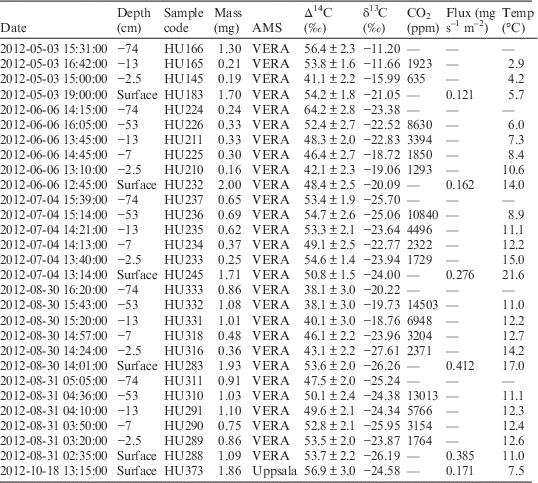
The collected samples were graphitized with Fe/Zn reduction (Slota et al. Reference Slota, Jull, Linick and Toolin1987) in the Laboratory of Chronology, University of Helsinki, and measured at three AMS laboratories to the precision of 1.3–3.0‰, depending on the laboratory and the mass of the sample. The laboratories were the Vienna Environmental Research Accelerator (VERA), the Tandem Laboratory at the University of Uppsala, and Helsinki Accelerator Mass Spectrometry Facility (HAMS) at the University of Helsinki. The δ13C values shown in the tables were measured with an Isotope Ratio Mass Spectrometer (ThermoQuest Finnigan) from CO2 prior to graphitization, as these best describe the original δ13C of the target (no effects from the AMS ion source). The fractionation correction for the radiocarbon results (see section below) were done with AMS-measured δ13C for the VERA results, and with the MS-measured for the HAMS and Uppsala results. The uncertainties of the δ13C values are 0.2‰ unless otherwise stated.
Units and Definitions
All 14C results are given as Δ14C values,
 $$\Delta ^{{14}} {\rm C}{\equals}\left[ {\rm F^{{14}} \rm C{\times}{\rm e}^{{{\minus}\lambda (y{\minus}1950)}} {\minus}1} \right]{\times}1000$$
where
 $$\rm F^{{14}} \rm C{\equals}A_{{{\rm sample}}} \,/\,\left( {0.95A_{{{\rm standard}}} } \right)$$
and denotes the ratio of measured and δ13C-corrected 14C/C ratios of a sample and oxalic acid standard (Reimer et al. Reference Reimer, Brown and Reimer2004), y is the year of measurement and
 $\lambda {\equals}1\,/\,8267\,{\rm y}^{{{\minus}1}} $
is the decay constant of radiocarbon. The δ13C-correction for the samples was performed in the standard way given by (Stuiver and Polach Reference Stuiver and Polach1977) to –25‰. It is used to correct for natural isotopic fractionation of the 14C/C ratios based on the measured 13C/12C ratios.
Quality Control
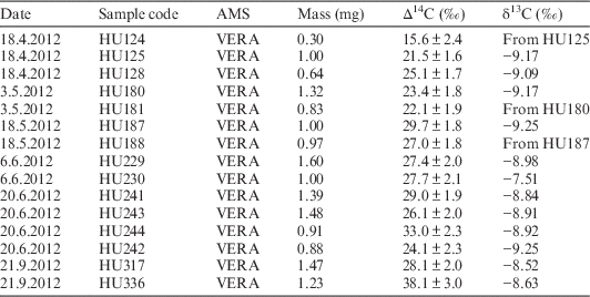
The reliability of the sieve collection for CO2 samples has been verified under laboratory conditions (Palonen Reference Palonen2013). The reliability of gas sample graphitization and AMS measurements was tested prior to sampling with several standards, the results of which were within 2 standard errors (1.9‰) from the reference value. To check the quality of the results for real field-collected samples, several 7-min sequential samples were taken from the same height (125 m) in the beginning of the measurement campaign. The results are given in Table 1. The duplicates give consistent Δ14C and δ13C values within their uncertainties. For the subsequent figures and tables, average values of individual measurements were used when sequentially sampled CO2 samples were done.
Results from multiple samples of the atmosphere on the same date. Some δ13C values have been measured only once for two samples.

For the later batches of samples, we noticed a slight carbon contribution (up to 0.4% of normal sample current, with 14C concentration of 0.12 fraction modern) coming from iron powder used in the graphitization step of sample preparation. Because the standard samples go through the same preparation process, the results from most samples are unaffected by the small amount of extra carbon. However, results from soil profile samples with small carbon mass had to be corrected for this extra carbon. Corrected values are shown in the figures, and both uncorrected and corrected values are given in Table 3. For the corrected values, the uncertainties are given as half of the difference between the original and corrected value.
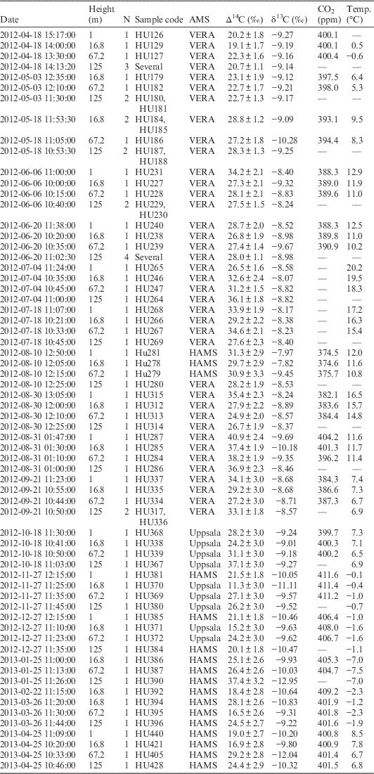
Atmospheric results for different dates and heights. Some values represent averages of N measurements. Samples were measured at three AMS facilities: VERA=Vienna Environmental Research Accelerator, HAMS=Helsinki Accelerator Mass Spectrometry Facility, Uppsala=Tandem Laboratory, University of Uppsala. CO2 concentrations were measured with Li-Cor LI-840 infrared light absorption analyzer and the air temperatures with Pt100 sensors at corresponding heights.

RESULTS
Δ14C-CO2 Values in the Atmosphere
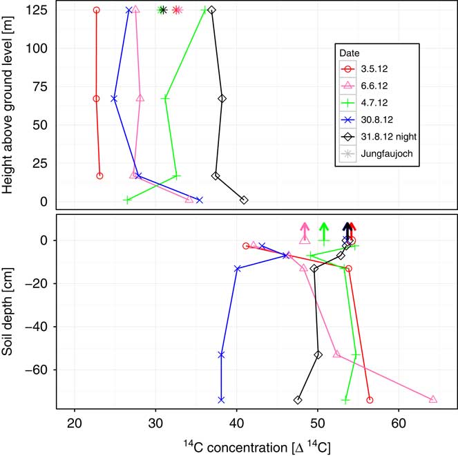
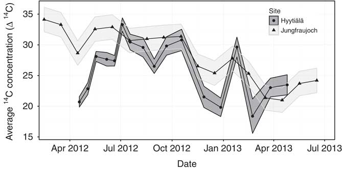
Δ14C-CO2 in the atmosphere varied between 20 to 38‰ (Figure 1 and Table 2). There was no vertical gradient observed in the Δ14C above the canopy (i.e. >16 m agl). The results from 16.8-, 67.2-, and 125-m heights were consistently within the uncertainty values of the measurements. The Δ14C values at 1-m height were close to the values observed higher in the atmosphere but in some cases the 1-m value was shifted towards the higher Δ14C values of soil-emitted CO2 (arrows in Figure 1). There was a significant difference between the nighttime and daytime measurements in August, with the nighttime values being roughly 11‰ higher compared to the daytime values. The average Δ14C calculated from the 16.8-, 67.2-, and 125-m heights showed a 10±0.5‰ seasonal variation with the highest Δ14C values observed during late summer and autumn and the lowest values in the winter and spring (Figure 2).
Δ14C-CO2 values of atmospheric (top) and soil air (bottom) as a function of height. Symbols with arrows represent the Δ14C values of soil emission. Asterisks represent corresponding Δ14C values at Jungfraujoch, Swiss Alps.

Average atmospheric 14C level in Finland compared to the measurements from the Swiss Alps (Levin and Hammer, unpublished data). While the present data are only one year long, they seem to point to larger seasonal variation in the northern latitudes.

Δ14C-CO2 Values in Soil Air and in Soil CO2 Emissions
The Δ14C values measured in soil CO2 ranged mostly from 37 to 65‰ (Figure 1 and Table 3). High soil water content prevented taking a representative sample in some of the tubes during late autumn and early spring. The Δ14C values were highest in spring and decreased significantly in autumn (Figure 1). This seasonal change was most notable in the deep soil. The difference between the nighttime and daytime Δ14C results (late August) was pronounced, the nighttime results having 10‰ larger values than the daytime ones.
Soil results for different dates and depths. For chamber-collected samples, the flux has been calculated with the HMR procedure for CO2 values exceeding 390 ppm. Soil temperature was measured with Philips KTY81-110 temperature sensors at corresponding depths.

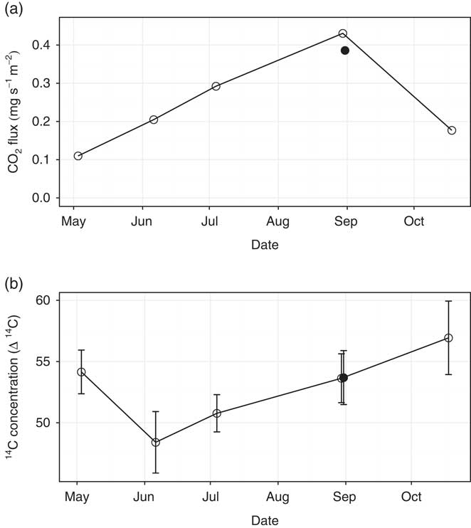
The chamber measurements showed an increase in the CO2 emissions from May to late August (Figure 3a), while a high Δ14C value in the emission was recorded in early May, followed by a drop and a steady increase up to October (Figure 3b). In August, the Δ14C in the CO2 emission during nighttime was almost equal to the daytime value (Figure 3b) while the total CO2 flux decreased (Figure 3a) and Δ14C values increased in humus and 1 m above the soil surface (Figure 1) during the night.
The CO2 flux (a) and Δ14C in it (b). Error bars depict one standard error. Solid circles represent the nighttime values.

DISCUSSION
Atmospheric Results
While the vertical gradient in the atmospheric Δ14C signal above the canopy was relatively constant from 16.7 m to 125 m height, the Δ14C value in air collected close to the ground (1 m) in the forest canopy was obviously affected by the 14C-elevated soil emission signal. This effect should be kept in mind when free tropospheric 14CO2 levels shall be derived from air samples that are collected close to the ground. Depending on atmospheric mixing conditions, they may deviate from a real representative 14C-CO2 level, in our case of air sampled more than 100 m above the canopy by up to +10‰. Consequently, as shrubs and other forest floor vegetation incorporate (via photosynthesis) the CO2 close to the soil surface, they likely incorporate a higher 14C value than from the free troposphere. This is important to keep in mind when dating recent materials with 14C.
The nighttime atmospheric Δ14C-CO2 profile in August 2012 was on average consistently 11‰ higher than the daytime profile. This result may have been caused by the diurnal changes in the atmospheric boundary layer (ABL) height (Garratt Reference Garratt1992). During the day, the atmosphere is heated from below by the absorption of sunlight, resulting in convective mixing of the air masses up to the height 1 or 2 km. During the night, the absence of sunlight and hence convection results in a shallow nocturnal boundary layer (NBL), in which mixing is mainly caused by wind friction. This layer is usually between 100 and 300 m thick. Within the NBL, CO2 from soil respiration with higher Δ14C values is mixed with atmospheric air. Indeed, effects of soil respiration are observed up to the 125 m height based on the Δ14C signature for the night. This is in line with similar results from other studies (Phillips et al. Reference Phillips, McFarlane, LaFranchi, Desai, Miller and Lehman2015; LaFranchi et al. Reference LaFranchi, McFarlane, Miller, Lehman, Phillips, Andrews and Tans2016).
However, a simple mass balance, calculating the amount of soil CO2 required explaining the observed Δ14C increase during night in an air column up to 125 m height yields approximately 100 g. Comparing this to the amount of CO2 from soil emission (Figure 3, i.e. 14 g over 10 hr), the direct contribution from soil emission cannot be solely responsible for the 14C shift. We therefore conclude that the system is more complex. Also, the present study has only one set of nighttime measurements, therefore, it would be premature to draw further conclusions. Indeed, a full quantitative explanation for the high atmospheric nighttime Δ14C values will likely require detailed micrometeorological and ecosystem-level modeling and further experimental work targeting this particular question.
The 10±0.5‰ seasonal variation in Δ14C in the present atmospheric data is significantly larger than the average 4‰ at Jungfraujoch (Levin et al. Reference Levin, Kromer and Hammer2013). The larger seasonal variation at this higher-latitude lower tropospheric site may be caused by the strong seasonality of soil respiration in higher latitudes, which has an elevated 14C signal (see Figure 1; LaFranchi et al. Reference LaFranchi, McFarlane, Miller, Lehman, Phillips, Andrews and Tans2016). Alternatively, it may reflect the fact that, due to the deflection of cosmic rays by the earth’s magnetic field, roughly four times more 14C is produced in the stratosphere and the troposphere near the geomagnetic poles compared to the equator (Lingenfelter Reference Lingenfelter1963).
Soil Results
Root and rhizosphere respiration arises from the growth and maintenance of plant roots and microbial utilization of labile root exudates. It can be assumed to have the Δ14C signature close to that of the atmosphere since it is mainly originating from the recently assimilated carbon (Högberg and Read Reference Högberg and Read2006) having an average Δ14C value of 27‰ in our study. The Δ14C of the Rd depends mainly on the age of soil organic matter (SOM), which is variable but can be hundreds or up to some thousands of years old especially in the lower mineral soil horizons (Liski et al. Reference Liski, Ilvesniemi, Mäkelä and Starr1998). In another project, Δ14C in the SOM collected from a similar site 5 km away from the site used in this study indicated that the C in the upper organic soil horizon was on average approximately 30 yr old (Lindén et al. Reference Lindén, Heinonsalo, Buchmann, Oinonen, Sonninen, Hilasvuori and Pumpanen2014). This means that SOM mainly originates from the post-bomb period of over-modern but with decreasing Δ14C in the atmosphere. Based on trenching experiments performed at the current site (unpublished data), we can estimate by a linear extrapolation from measurements carried out in 2013–2015 that the Δ14C value of Rd would be around (70±10)‰ in the year 2012.
We expected that the Δ14C values in soil air CO2 and soil CO2 efflux would be different in early summer compared to late summer. The Δ14C values especially in the deeper soil layers decreased towards the end of the autumn by up to 15‰ units relative to the values measured in spring i.e. they approached atmospheric values. This could be an indication of changes in the origin of CO2 suggesting an increase in tree root activity and a larger share of autotrophic respiration (including rhizosphere respiration) in total soil CO2 emissions. This is in line with (Pumpanen et al. Reference Pumpanen, Kulmala, Lindén, Kolari, Nikinmaa and Hari2015) who determined the autotrophic respiration at the same site to be highest in late July and early August when also the highest fine root biomass occurs. Also Phillips et al. (Reference Phillips, McFarlane, Risk and Desai2013) measured Δ14C-CO2 soil profiles in a hardwood forest in Wisconsin, USA, and found respired Δ14C-CO2 to decline throughout the summer in intact plots, shifting from an older C composition to younger one. At the same time, respired Δ14C-CO2 from plots excluding living tree roots remained comparatively higher than that in intact plots and thus, we can expect that the decline in the intact plots was caused by the increase in autotrophic respiration having Δ14C-CO2 levels close to ambient. In addition, microbes likely shift sources from older SOM in early summer and spring toward more recently fixed carbon in summer when plants and plant roots are more active. This would influence particularly the lower depths of the profile, where autotrophic respiration is not as large.
On the other hand, we observed an increase in the Δ14C values in the surface soil, i.e. in the measured soil emissions towards the end of the summer. This may be partly explained also by root zone and rhizosphere activity. Most of the biologically active organic matter in this forest stand is accumulated in the topsoil, organic soil layers and upper centimeters of the mineral soils, and a large part of the material in the organic layer has accumulated only after the forest stand was regenerated and exposed to prescribed burning in 1962. However, SOM also contains older carbon in recalcitrant fractions, which are resistant to decomposition. This material also contains large amounts of nitrogen, which is bound in SOM matrix and not easily available for the use of living vegetation (Korhonen et al. Reference Korhonen, Pihlatie, Pumpanen, Aaltonen, Hari, Levula, Kieloaho, Nikinmaa, Vesala and Ilvesniemi2013). In most boreal forests, nitrogen is a growth limiting factor and for acquiring nutrients, trees need to allocate large amounts of carbohydrates belowground to microbes e.g. ectomycorrhizal fungi, which are using it for producing extracellular enzymes to degrade SOM (Heinonsalo et al. Reference Heinonsalo, Sun, Santalahti, Bäcklund, Hari, Pumpanen and Post2015; Kieloaho et al. Reference Kieloaho, Pihlatie, Carrasco, Kanerva, Parshintsev, Riekkola, Pumpanen and Heinonsalo2016). In addition, we showed recently in a microcosm experiment that the mineralization of old SOM was significantly increased in the presence of living root system having active ectomycorrhizal fungi (Lindén et al. Reference Lindén, Heinonsalo, Buchmann, Oinonen, Sonninen, Hilasvuori and Pumpanen2014). This was observed as increasing age in soil respiration measured with Δ14C. Thus, it seems evident that the root activity induces decomposition of older SOM fraction in the topmost soil layers that is seen in this study as an increase in Δ14C in soil CO2 emissions even if the root activity in deep soil decreased Δ14C throughout the season.
The Δ14C values near the soil surface were closer to the atmospheric values than those measured in the chamber i.e. CO2 emissions. This remains unsolved but may be due to high spatial variation in root biomass and amount of SOM and its quality. Even if the chamber measured the emissions nearby the profile, the CO2 production rates and the origin might have differed. Another possibility is that atmospheric air entered the profile tube, although the δ13C values measured from the tubes (Table 3) do not seem to support this. In addition, the estimated sampling volume of soil air after the CO2 removal roughly corresponds to a cylinder with 3.3 cm radius around the profile tubes, thus the air collected from the tubes was mostly originating from the organic layer.
The difference in the Δ14C values in soil CO2 in August was significant between day and night. This is likely the result of changes in the shares of Rd and Rr. Savage et al. (Reference Savage, Davidson and Tang2013) showed that autotrophic respiration has a diurnal cycle in a middle aged hardwood forest in Massachusetts, USA, and Kodama et al. (Reference Kodama, Barnard, Salmon, Weston, Ferrio, Holst and Werner2008) found diurnal changes in the relative share of autotrophic and heterotrophic respiration in a temperate Scots pine forest in Germany. Also, in our study, the decrease in the amount of photosynthates entering the roots, root zone, and rhizosphere activity decreases during night more than the decomposition of SOM. The time delay between photosynthesis and soil CO2 efflux depends on the transfer time of carbohydrates in the phloem and most studies conducted by pulse labeling with isotopes have shown time lags from few hours to 5 days between photosynthesis and soil respiration (Mencuccini and Hölttä Reference Mencuccini and Hölttä2010). However, those results describe the transfer time of actually assimilated C molecules while the changes in photosynthesis rate may also be reflected to Rr through pressure propagation in the phloem with a much shorter time delay (Mencuccini and Hölttä Reference Mencuccini and Hölttä2010). Also, the size of carbohydrate pool within the plants may affect the magnitude and time delay of changes in soil CO2 efflux following changes in photosynthesis. Big plants such as trees having larger carbohydrate pools have longer time delay between photosynthesis and belowground respiration while shrub and herbaceous vegetation with smaller structural C pools have shorter time delay. In a recent study (Kulmala L, unpublished results) it was shown that for underground vegetation plants, mainly ericoid dwarf shrubs, the day-night difference in the autotrophic respiration was significant, even after some minutes in darkness the belowground respiration was significantly decreased. This could mean that in our case, ericoid plant species could have an influence on the observed differences in the Δ14C values in soil CO2 in August between day and night. There was also a notable difference in the soil temperature, which likely affects heterotrophic and autotrophic soil respiration differently (Ekblad et al. Reference Ekblad, Boström, Holm and Comstedt2005; Heinemeyer et al. Reference Heinemeyer, Hartley, Evans, Carreira De La Fuente and Ineson2007). However, the diurnal cycle of respiration components in boreal Scots pine forest soil still requires further study.
CONCLUSIONS
We collected CO2 from different parts of a forest ecosystem with a portable sampling system using molecular sieve cartridges to selectively trap the CO2 in the target gas. The results represent the first larger ecosystem-level Δ14C dataset from northern Europe.
The atmospheric samples of the present study show a large seasonality in the Δ14C-CO2 in northern Europe. The consistently higher Δ14C values at night suggest a significant contribution of 14C-enriched CO2 that could be observed up to 125 m height. A partial explanation for this is the increased proportion of CO2 from soil emission due to reduced vertical mixing of air during night, but this alone seems not to be able to explain the large difference compared to daytime values. Further research is needed to explain the observed large diurnal variation in detail.
With the soil air and soil CO2 efflux Δ14C-CO2 measurements, we observed an increase in the Δ14C values in the surface soil CO2 towards the end of the summer. We attribute this to increasing root activity, which then induces decomposition of older SOM fraction at the site, the conclusion being supported by other studies performed at the site. On the other hand, a decreasing seasonal trend was observed in Δ14C for the lower depths in the forest soil, likely caused by an increase in autotrophic respiration up to August.
We also observed a large diurnal variation in soil-air Δ14C-CO2. Here, the Δ14C values reflect the changes in the shares of autotrophic and heterotrophic respiration, with the root activity decreasing during the night more than the decomposition of soil organic matter. However, the proportions of Δ14C signals from autotrophic or heterotrophic CO2 sources at the different soil depths are presently unknown. This deserves further research as more knowledge on the priming of SOM and changes in boreal forest soil C pools is necessary for reliable soil C modeling.
ACKNOWLEDGMENTS
This work was mainly funded by the Academy of Finland project MIRA (139036). Support and funding also came from Academy of Finland projects 1292699, 277623, and 285630, and from the Academy of Finland Centre of Excellence (118780) and ICOS-Finland (281255). We wish to thank the personnel in the SMEAR II station for providing technical support for sample collection from the atmosphere and from the soil chambers. The staff at the Laboratory of Chronology, Finnish Museum of Natural History (LUOMUS) is gratefully acknowledged for significant help in sample treatment. P. Steier and R. Zorro are gratefully acknowledged for performing the AMS measurements at VERA and Uppsala AMS laboratories, respectively. The technical personnel at the Accelerator Laboratory, Department of Physics, University of Helsinki are greatly acknowledged for their technical support in the AMS measurements performed at HAMS during the project.