The scattering of electromagnetic waves from circular cylinders buried below a flat interface has been studied by many authors because of their important applications in the microwave and optical regimes [Reference D’Yakonov1–Reference Lawrence and Sarabandi24]. This study finds applications in the detection of hidden land mines, pipes, conduits, other intriguing buried things, skin tumors, vessels, and fibers immersed in biological tissues, etc. Diffraction of electromagnetic waves by a circular cylinder in a homogeneous half-space has been discussed by Yakonov [Reference D’Yakonov1]. The problem of electromagnetic scattering from cylinders of arbitrary cross-section in a conductive half-space has been solved by Parry and Ward [Reference Parry and Ward2]. The mode-matching technique has been used by Howard [Reference Howard3] to solve a two-dimensional integral equation for the scattered field. Ogunade [Reference Ogunade4] extended an early work of Yakonov [Reference D’Yakonov1] to obtain numerical results in an easy way. Mahmoud and co-workers [Reference Mahmoud, Ali and Wait5] have used a set of multipole-induced line sources of electric and magnetic type to find the scattered field from a buried circular cylinder inside a lossy earth. An approximate scattering solution of a buried low dielectric contrast cylinder based on the Born approximation has been discussed by Hill [Reference Hill6]. Hongo and Hamamura [Reference Hongo and Hamamura7] developed the asymptotic solutions for plane-wave scattering by a cylindrical obstacle buried in a dielectric half-space, which were later corrected by Naqvi and co-workers in [Reference Naqvi, Rizvi and Yaqoob8]. Scattering characteristics of a buried dielectric cylinder in a grounded dielectric layer and a deeply buried perfectly conducting cylinder have been investigated by Naqvi et al. [Reference Naqvi and Rizvi9, Reference Naqvi, Rizvi and Yaqoob10]. A spectral domain scattering from a single buried perfectly conducting cylinder [Reference Ciambra, Frezza, and and Schettini11], multiple buried perfectly conducting cylinders [Reference Di Vico, Frezza, Pajewski and Schettini12], and multiple buried dielectric cylinders [Reference Di Vico, Frezza, Pajewski and Schettini13] in a dielectric half-space have been studied. A scattering problem of three-dimensional source excitation of a buried circular cylinder in soil has been solved by Hansen and Meincke [Reference Hansen and Meincke14] using the fast Fourier transform technique. The cylindrical wave approach has been used by Frezza et al. to study the scattering from the buried isolated metallic cylinder [Reference Frezza, Pajewski, Ponti and Schettini15] and multiple buried metallic cylinders [Reference Frezza, Pajewski, Ponti, Schettini and Tedeschi16]. Nasr and co-workers [Reference Nasr, Eshrah and Hashish17] have adopted an exact and fast analytical method based on a multiple reflections approach to study the scattering from buried metallic or dielectric cylindrical objects. Scattering properties of various types of circular cylinders, including perfect electromagnetic conductor (PEMC) [Reference Ahmed and Naqvi18, Reference Hamid and Cooray19], topological insulator [Reference Akhtar, Naz, Fiaz and Naqvi20], topological insulator-coated PEMC [Reference Fiaz21], and buried below a flat interface, have been explored recently. The cylindrical wave approach in the time domain has been used to study the scattering from buried multiple dielectric cylinders in the microwave [Reference Ponti, Santarsiero and Schettini22] and optical [Reference Ponti, Santarsiero and Schettini23] regimes. Lawrence and Sarabandi [Reference Lawrence and Sarabandi24] have used the plane-wave representations of fields to study the scattering from a buried dielectric cylinder which is placed below a slightly rough or flat interface.
The concept of metamaterial (MM) originated from Veselago’s work [Reference Veselago25], which suggested a material with negative permittivity and permeability. These types of MMs do not exist in nature, but they can be realized artificially. Nowadays, the study of these MMs has gained attention because of their potential practical engineering applications [Reference Pendry, Holden, Stewart and Youngs26–Reference Raqeeb, Awan and Hussain56]. Based on Veselago’s work, Pendry and co-workers [Reference Pendry, Holden, Stewart and Youngs26] give the concept of realizing a negative permittivity material, or epsilon-negative (ENG) MM, based on the periodic arrangement of metallic wires. Likewise, the realization of a negative permeability material, or mu-negative (MNG) MM, based on metallic split-ring resonators has also been proposed by Pendry et al. [Reference Pendry, Holden, Robbins and Stewart27]. The design of an MM with simultaneous negative permittivity and negative permeability has been proposed by Smith et al. [Reference Smith, Padilla, Vier, Nemat-Nasser and Schultz28] and Shelby et al. [Reference Shelby, Smith and Schultz29], which is now called double negative (DNG) or left-handed MM in the literature. Later on, various studies on ENG, MNG, and DNG MMs have been conducted by many authors [Reference Alú and Engheta30–Reference Awan, ullah, ullah and Ashraf38]. Engheta et al. [Reference Engheta, Alu, Silveirinha, Salandrino and Li39] introduced the concept of epsilon-near-zero (ENZ), mu-near-zero (MNZ), and double-near-zero (DNZ) MMs. For an ENZ MM, its permittivity is nearly zero, and for an MNZ MM, its permeability is nearly equal to zero. The combination of ENZ and MNZ MMs gives the DNZ MM, which supports propagating modes at an extremely large wavelength. Such types of MMs with nearly zero electromagnetic parameters are useful in the design of energy tunneling [Reference Silveirinh and Engheta40–Reference Liu, Cheng, Hand, Mock, Cui, Cummer and Smith42], wavefront shaping [Reference Alù, Silveirinh and Engheta43, Reference Wang and Huang44], directive emission [Reference Gao, Sun, Deng, Mathai, Gangopadhyay and Yang45, Reference Pacheco-Pena, Torres, Beruete, Cia and Engheta46], and cloaking [Reference Guo, Jiang, Zhu, Sun, Li and Chen47]. Some interesting applications of these near-zero MMs have been discussed in [Reference Huang, Lai, Hang, Zheng and Chan48–Reference Raqeeb, Awan and Hussain56].
Recently, various types of cylindrical metasurfaces (MSs) have been considered due to their important microwave and optical engineering applications [Reference Sipus, Bosiljevac and Grbic57–Reference Krasnok and Alú67]. Scattering characteristics of various MS-covered circular cylinders have been investigated by some authors [Reference Sipus, Bosiljevac and Grbic57–Reference Awan, Ahmad, Khan and Hussain59]. Cylindrical MSs are often used as a coating layer for various types of circular cylinders and find applications in cloaking [Reference Padooru, Yakovlev, Chen and Alú60–Reference Jiang and Werner63], camouflage [Reference Vellucci, Monti, Toscano and Bilotti64], illusions [Reference Jiang and Werner65, Reference Safari, Kazemi, Abdolali, Albooyeh and Capolino66], and bound states in the continuum [Reference Krasnok and Alú67]. According to the authors, no one has studied the scattering characteristics of buried MM cylinders, including ENG, MNG, DNG, ENZ, MNZ, and DNZ MMs, and buried MS-covered MM cylinders below a flat interface under transverse magnetic (TM) and transverse electric (TE) incident polarizations. Likewise, the scattering properties of a buried MS-covered frequency-dispersive DNG MM cylinder and their comparisons with the scattering characteristics of a buried frequency-dispersive DNG MM cylinder without MS have not been reported previously in the literature by considering TM and TE incident polarizations. These scattering characteristics have been studied in the current paper.
In this paper, the scattering properties of an MM circular cylinder covered with a lossless MS and buried below a flat interface are explored. In order to study the complete scattering characteristics, both types of incident polarization, i.e., TM and TE, have been considered. By using the concept of double-sided impedance boundary conditions, the unknown scattering coefficients from the MS-covered MM circular cylinder have been derived, which have not been found previously in the literature. Later on, by taking into account the multiple interactions between the MS-covered circular cylinder and the interface, the total scattered-reflected field in the region above the flat interface is found based on the procedure as outlined by Lawrence and Sarabandi [Reference Lawrence and Sarabandi24]. Finally, the scattering width (SW) of the considered buried circular cylinder is calculated, which is a quantity of interest in the present study. The influences of various parameters, including the radius and depth of the considered MM circular cylinders and the surface impedance of the MS, upon the scattering characteristics have been investigated. As a general remark, it is argued that the SWs of buried MM circular cylinders can be enhanced or diminished by varying the surface reactance of the MS. During the study, it was found that the buried considered MM cylinders and specific capacitive MS-covered considered MM cylinders have enhanced SW as compared to the SW of a buried dielectric cylinder as adopted in [Reference Lawrence and Sarabandi24] under TM and TE incident polarization while keeping all geometrical parameters the same. It is shown that the SWs of the buried considered inductive MS-covered ENG and ENZ cylinders are greater than their corresponding SWs of buried ENG and ENZ cylinders without MS under TM incident polarization. It is argued that the considered inductive MS can be used to enhance the SW of a buried MS-covered MNZ cylinder as compared to the SW of a buried MNZ cylinder without MS under TE incident polarization. In the case of a buried MS-covered DNZ cylinder, it is further investigated that the considered capacitive MSs can be used to enhance the SW of a buried DNZ cylinder for both types of incident polarization. These enhanced scattering characteristics provide interesting results which are helpful in the design of electromagnetic or optical detection systems for buried objects. Likewise, specific MSs with surface reactances of  $\pm$0.01 and
 $\pm$0.1 k
 $\Omega$ can be used to reduce the SW of a buried MS-covered DNG cylinder as compared to the SW of a buried DNG cylinder without MS under TE wave incidence. These reduced scattering findings have applications in the design of stealth systems. Later on, backscattering characteristics have been explored. In the case of buried considered MM cylinders without MS, it is observed that the minimum backscattering is achieved for a buried DNZ cylinder under TM wave incidence, and the maximum backscattering is found for a buried DNG cylinder under TE wave incidence. It is shown that a specific MS with a surface reactance of
 $-$696
 $\Omega$ can be used to significantly enhance the backscattering from a buried DNZ cylinder. Likewise, it is shown that an MS with a surface reactance of
 $-$169
 $\Omega$ can significantly reduce the backscattering from a buried DNG cylinder. It is further shown that two different buried MM cylinders, i.e., ENG and ENZ cylinders having the same size with different values of MS reactances, have the same backscattering characteristics. These same backscattering characteristics with different MMs and MSs may find applications in electromagnetic or optical illusions. These above-mentioned findings have not been reported previously in the literature and signify the novelty of the present study.
Analytical formulation
An infinite-length circular cylindrical object with electromagnetic properties of  $\epsilon_{2} = \epsilon_{0}\epsilon_{r2}$ and
 $\mu_{2} = \mu_{0}\mu_{r2}$ is considered, where
 $\epsilon_{0}$ and
 $\mu_{0}$ are the permittivity and permeability of the free space, respectively. Likewise, the parameters
 $\epsilon_{r2}$ and
 $\mu_{r2}$ represent the relative permittivity and relative permeability of the material cylinder, respectively, which occupies region 2. It has a radius of
 $a$. This circular cylinder is covered with an infinitesimally thin cylindrical MS. This cylindrical MS is modeled by a complex surface impedance dyad
 $\overline{\overline{Z}}$ in the usual cylindrical coordinates
 $(\rho,\phi,z)$ as below,
 \begin{equation}
\overline{\overline{\textbf{Z}}}
= \begin{bmatrix}
Z_{\phi\phi} & 0\\
0 & Z_{zz}\\
\end{bmatrix}
= \begin{bmatrix}
Z_{e} & 0\\
0 & Z_{m}\\
\end{bmatrix}
\end{equation}
where  $Z_{m}$ =
 $Z_{\mathrm{TM}}$ =
 $R_{m}$ + j
 $\chi_{m}$ and
 $Z_{e}$ =
 $Z_{\mathrm{TE}}$ =
 $R_{e}$ + j
 $\chi_{e}$. Here,
 $Z_{m}$ corresponds to the equivalent surface impedance for the TM mode, whereas
 $Z_{e}$ represents the equivalent surface impedance for the TE mode. The real parts of
 $Z_{m}$ and
 $Z_{e}$, i.e.,
 $R_{m}$ and
 $R_{e}$, represent losses present in the MS. The imaginary parts of
 $Z_{m}$,
 $Z_{e}$, i.e.,
 $\chi_{m}$,
 $\chi_{e}$, represent the respective surface reactances of the MS. For inductive reactances, we have
 $\chi_{m}$,
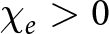 $\chi_{e} \gt 0$. Likewise, in the case of
 $\chi_{m}$,
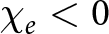 $\chi_{e} \lt 0$, we have capacitive reactances. A time convention of
 $e^{j\omega t}$ has been adopted in the present study. This MS-covered circular cylinder is buried below the flat interface. The depth of a circular cylinder below the flat interface is taken to be
 $d$. Region 0 is taken to be the region which is above the interface and assumed to be the free space. This region is characterized by the free-space wavenumber
 $k_{0}$ =
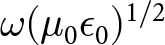 $\omega(\mu_{0}\epsilon_{0})^{1/2}$ and the free-space intrinsic impedance
 $\eta_{0}$ =
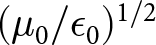 $(\mu_{0}/\epsilon_{0})^{1/2}$. Region 1 is the medium below the interface and has the electromagnetic parameters of
 $\epsilon_{1}$ =
 $\epsilon_{0}\epsilon_{r1}$ and
 $\mu_{1}$ =
 $\mu_{0}\mu_{r1}$, where
 $\epsilon_{r1}$ and
 $\mu_{r1}$ are the relative permittivity and relative permeability of region 1, respectively. Here
 $k_{1}$ =
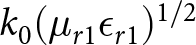 $k_{0}(\mu_{r1}\epsilon_{r1})^{1/2}$ and
 $\eta_{1}$ =
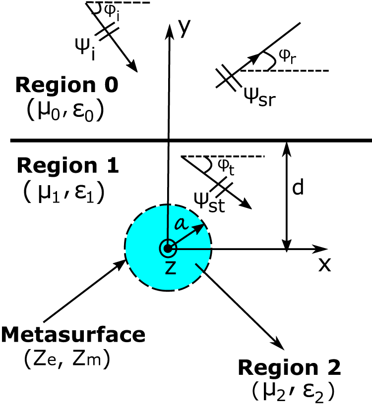
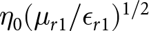 $\eta_{0}(\mu_{r1}/\epsilon_{r1})^{1/2}$. The geometrical configuration of the problem is shown in Figure 1.
The geometrical configuration of an MS-covered MM circular cylinder buried below a flat interface.

(1) Long description
A metasurface-covered circular cylinder buried below a flat interface. The interface separates Region 0, characterized by mu subscript 0 and epsilon subscript 0, from Region 1, characterized by mu subscript 1 and epsilon subscript 1. Region 0 is above the interface, while Region 1 is below it. The cylinder is located in Region 1, with its center marked by the letter z and radius labeled as a. The depth of the cylinder below the interface is indicated by the letter d. The metasurface is associated with electromagnetic parameters Z subscript e and Z subscript m. Region 2, characterized by mu subscript 2 and epsilon subscript 2, is shown below the cylinder. Arrows labeled psi subscript i, psi subscript sr and psi subscript st represent different electromagnetic fields, with corresponding angles phi subscript i, phi subscript r and phi subscript t. The x and y axes are marked, with the y-axis pointing upwards and the x-axis pointing to the right.
It is initially considered that there is no flat interface, and an MS-covered cylinder is placed in a background medium with electromagnetic parameters of  $\epsilon_{1}$ and
 $\mu_{1}$. To study the complete scattering properties, both types of incident wave polarizations, i.e., TM and TE, have been considered. This MS-covered cylinder is illuminated by a plane wave, which travels in a direction that makes an angle
 $\phi_{i}$ with the
 $+x$-axis. For the TM polarization, the
 $z$-components of the incident electric field
 $E^{i}_{z}$, the scattered electric field
 $E^{s}_{z}$, and the internal electric field
 $E^{in}_{z}$ inside the cylinder can be written in terms of cylindrical coordinates (
 $\rho$,
 $\phi$,
 $z$) as below [Reference Balanis68, Reference Awan, Raqeeb and Hussain69],
 \begin{align}
E^{i}_{z} & = E_{o}e^{-jk_{1}\rho\cos(\phi - \phi_{o})}=E_{o}\sum_{n = -\infty}^{n = +\infty}j^{-n}J_{n}(k_{1}\rho)\\ \nonumber &\quad \cdot e^{-jn(\phi-\phi_{i})}\end{align}
 \begin{equation}
E^{s}_{z} = E_{o}\sum_{n = -\infty}^{n = +\infty}j^{-n}C^{TM}_{n}H^{(2)}_{n}(k_{1}\rho)e^{-jn(\phi-\phi_{i})}
\end{equation}
 \begin{equation}
E^{in}_{z} = E_{o}\sum_{n = -\infty}^{n = +\infty}j^{-n}A^{TM}_{n}J_{n}(k_{2}\rho)e^{-jn(\phi-\phi_{i})}
\end{equation}
where  $E_{o}$ is a constant magnitude of the incident electric field. The functions
 $J_{n}(\cdot)$ and
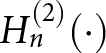 $H^{(2)}_{n}(\cdot)$ represent the
 $n$th order Bessel function of the first kind and
 $n$th order Hankel function of the second kind, respectively. It should be noted that
 $k_{2}$ =
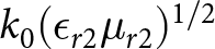 $k_{0}(\epsilon_{r2}\mu_{r2})^{1/2}$ and
 $\eta_{2}$ =
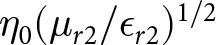 $\eta_{0}(\mu_{r2}/\epsilon_{r2})^{1/2}$. The coefficients
 $A^{TM}_{n}$ and
 $C^{TM}_{n}$ are unknowns and need to be determined. The
 $\phi$-components of the incident magnetic field
 $H^{i}_{\phi}$, the scattered magnetic field
 $H^{s}_{\phi}$, and the internal magnetic field
 $H^{in}_{\phi}$ can be found using Maxwell’s equations. The unknown coefficients
 $A_{n}$ and
 $C^{TM}_{n}$ can be found by applying the double-sided impedance boundary conditions [Reference Awan, Ahmad, Khan and Hussain59] at
 $\rho = a$ for
 $0\leq\phi\leq 2\pi$, which are given below,
 \begin{equation}
E_{z}^{in}= E_{z}^{i}+E_{z}^{s}
\end{equation}
 \begin{equation}
E_{z}^{in}=Z_{m}[H_{\phi}^{i}+H_{\phi}^{s}-H_{\phi}^{in}]
\end{equation}
By substituting the incident, scattered, and internal electric and magnetic field components into the boundary conditions given by Eqs. (5)–(6) and solving the resulting system of linear equations, we can find the unknown coefficients  $A^{TM}_{n}$ and
 $C^{TM}_{n}$. The unknown scattering coefficient
 $C_{n}^{TM}$, which is of interest to the scattered electric field, can be written as,
 \begin{align}
C_{n}^{TM}&=\Big[jJ_{n}(x_{1})J_{n}(x_{2})+Z_{m}\Big\{(\frac{1}{\eta_{2}})J_{n}(x_{1})J^{\prime}_{n}(x_{2}) \\ \nonumber &-(\frac{1}{\eta_{1}})J_{n}(x_{2})J^{\prime}_{n}(x_{1})\Big\}\Big]\Big/\Big[-jJ_{n}(x_{2})H^{(2)}_{n}(x_{1}) \\ \nonumber &+Z_{m}\Big\{(\frac{1}{\eta_{1}})J_{n}(x_{2})H^{(2)\prime}_{n}(x_{1})-(\frac{1}{\eta_{2}})J^{\prime}_{n}(x_{2}) \\\nonumber & \cdot H^{(2)}_{n}(x_{1})\Big\}\Big]\end{align}
where 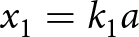 $x_{1}= k_{1}a$,
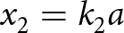 $x_{2}= k_{2}a$, and the prime
 $'$ shows the derivative with respect to the argument. In this case, if
 $Z_{m}$ = 0 and
 $k_2$ =
 $k_1$ =
 $k_0$, then this cylinder corresponds to a hollow perfect electric conductor (PEC) cylinder in the free-space background, and
 $C_{n}^{TM}$ becomes the same as that of the PEC cylinder [Reference Balanis68], which is given below,
 \begin{equation}
C_{n}^{TM}=\frac{-J_{n}(k_{0}a)}{H^{(2)}_{n}(k_{0}a)}
\end{equation}
On the other hand, if 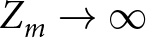 $Z_{m}\rightarrow\infty$, then no current is induced on the MS, and this special case is representative of a material cylinder without MS. In this case,
 $C_{n}^{TM}$ becomes the same as given in [Reference Lawrence and Sarabandi24], i.e.,
 \begin{equation}
C_{n}^{TM}=\frac{(1/\eta_{2})J_{n}(x_{1})J^{\prime}_{n}(x_{2})-(1/\eta_{1})J_{n}(x_{2})J^{\prime}_{n}(x_{1})}{(1/\eta_{1})J_{n}(x_{2})H^{(2)\prime}_{n}(x_{1})-(1/\eta_{2})J^{\prime}_{n}(x_{2})H^{(2)}_{n}(x_{1})}
\end{equation}
In the case of TE polarization, the  $z$-components of the incident magnetic field
 $H^{i}_{z}$, the scattered magnetic field
 $H^{s}_{z}$, and the internal magnetic field
 $H^{in}_{z}$ inside the cylinder can be written as,
 \begin{equation}
H^{i}_{z} = H_{o}\sum_{n = -\infty}^{n = +\infty}j^{-n}J_{n}(k_{1}\rho)e^{-jn(\phi-\phi_{i})}
\end{equation}
 \begin{equation}
H^{s}_{z} = H_{o}\sum_{n = -\infty}^{n = +\infty}j^{-n}C^{TE}_{n}H^{(2)}_{n}(k_{1}\rho)e^{-jn(\phi-\phi_{i})}
\end{equation}
 \begin{equation}
H^{1}_{z} = H_{o}\sum_{n = -\infty}^{n = +\infty}j^{-n}B^{TE}_{n}J_{n}(k_{2}\rho)e^{-jn(\phi-\phi_{i})}
\end{equation}
where  $H_{o}$ is a constant magnitude of the incident magnetic field. The
 $\phi$-components of the incident, scattered, and internal electric fields can be found using Maxwell’s equations. The unknown coefficients
 $B^{TE}_{n}$ and
 $C^{TE}_{n}$ can be found by applying the following double-sided impedance boundary conditions [Reference Awan, Ahmad, Khan and Hussain59] at
 $\rho = a$ for
 $0\leq\phi\leq 2\pi$,
 \begin{equation}
E_{\phi}^{in}=E_{\phi}^{i}+E_{\phi}^{s}\\
\end{equation}
 \begin{equation}
E_{\phi}^{in}=-Z_{e}[H_{z}^{i}+H_{z}^{s}-H_{z}^{in}]
\end{equation}
By substituting the required electric and magnetic field components in Eqs. (13)–(14) and following the same procedure as outlined for the TM case, the unknown scattering coefficient  $C_{n}^{TE}$ can be found, which is given as,
 \begin{align}
C_{n}^{TE}&=\Big[jJ^{\prime}_{n}(x_{1})J^{\prime}_{n}(x_{2})+Z_{e}\Big\{(\frac{1}{\eta_{1}})J_{n}(x_{1})J^{\prime}_{n}(x_{2}) \\ \nonumber &- (\frac{1}{\eta_{2}})J_{n}(x_{2})J^{\prime}_{n}(x_{1})\Big\}\Big]\Big/\Big[-jJ^{\prime}_{n}(x_{2})H^{{\prime}{(2)}}_{n}(x_{1}) \\ \nonumber &+ Z_{e}\Big\{(\frac{1}{\eta_{2}})J_{n}(x_{2})H^{{\prime}{(2)}}_{n}(x_{1})-(\frac{1}{\eta_{1}})J^{\prime}_{n}(x_{2}) \\ \nonumber & \cdot H^{(2)}_{n}(x_{1})\Big\}\Big]\end{align}
In the special case where  $Z_{e}$ = 0 and
 $k_2$ =
 $k_1$ =
 $k_0$, the MS-covered material cylinder becomes equivalent to a hollow PEC cylinder embedded in the free-space background. Using this information in Eq. (15), the scattering coefficient
 $C_{n}^{TE}$ becomes as,
 \begin{equation}
C_{n}^{TE}=\frac{-J_{n}^{\prime}(k_{0}a)}{H_{n}^{\prime}(k_{0}a)}
\end{equation}
which is the same as given by [Reference Balanis68, Reference Jin70]. Likewise, in the case where  $Z_{e}\rightarrow\infty$, then the MS-covered cylinder becomes equivalent to a material cylinder without MS. In this case,
 $C_{n}^{TE}$ becomes the same as given by Lawrence and Sarabandi [Reference Lawrence and Sarabandi24], i.e.,
 \begin{equation}
C_{n}^{TE}=\frac{(1/\eta_{1})J_{n}(x_{1})J^{\prime}_{n}(x_{2})-(1/\eta_{2})J_{n}(x_{2})J^{\prime}_{n}(x_{1})}{(1/\eta_{2})J_{n}(x_{2})H^{{\prime}{(2)}}_{n}(x_{1})-(1/\eta_{1})J^{\prime}_{n}(x_{2})H^{(2)}_{n}(x_{1})}
\end{equation}
Now we consider the geometry shown in Figure 1, where an MS-covered circular cylinder is buried below a flat interface. For this case, we consider both types of incident polarizations, i.e., TM and TE, and the incident field  $\psi_{0}^{i}$ is expressed as,
 \begin{equation}
\psi_{0}^{i}=e^{-j(k^{i}_{x}x-k^{i}_{0y}y)}
\end{equation}
where  $\psi$ is a scalar quantity, which corresponds to
 $E_{z}$ for the TM case and corresponds to
 $H_{z}$ for the TE case. For example,
 $\psi_{0}^{i}$ =
 $E_{z}^{i}$ for the TM case and
 $\psi_{0}^{i}$ =
 $H_{z}^{i}$ for the TE case for incident fields. Similar reasoning can be used for scattered and internal fields. Here
 $k_{0y}^{i}$=
 $[k_{0}^{2}-(k_{x}^{i})^{2}]^{1/2}$. The initial first-order reflected field
 $\psi_{0}^{r}$ from the interface boundary can be expressed in terms of a reflection coefficient
 $R_{01}^{L}$ as below,
 \begin{equation}
\psi_{0}^{r}= R_{01}^{L}(k_{x}^{i})e^{j2k_{0y}^{i}d}e^{-j(k^{i}_{{x}}x+k_{0y}^{i}y)}
\end{equation}
 \begin{equation}
R_{01}^{L}(k_{x}^{i}) = \left\{\begin{array}{ll}
\frac{k_{0y}^{i}-k_{1y}^{i}}{k_{0y}^{i}+k_{1y}^{i}}, & \textrm{TM polarization}\\
\frac{k_{1}^{2}k_{0y}^{i}-k_{0}^{2}k_{1y}^{i}}{k_{1}^{2}k_{0y}^{i}+k_{0}^{2}k_{1y}^{i}}, & \textrm{TE polarization}\\
\end{array} \right.
\end{equation}
with  $L$ = TM, TE and
 $k^{i}_{1y}$ =
 $[k_{1}^{2}-(k_{x}^{i})^{2}]^{1/2}$. Likewise, the first-order transmitted field
 $ \psi_{0}^{t}$ into region 1 can be expressed in terms of the transmission coefficient
 $T_{01}^{L}$ as below,
 \begin{equation}
\psi_{0}^{t}= T_{01}^{L}(k^{i}_{x})e^{j(k_{0y}^{i}-k_{1y}^{i})d}e^{-j(k_{x}^{i}x-k_{1y}^{i}y)}
\end{equation}
 \begin{equation}
T_{01}^{L}(k_{x}^{i}) = \left\{\begin{array}{ll}
\frac{2k_{0y}^{i}}{k_{0y}^{i}+k_{1y}^{i}}, & \textrm{TM polarization}\\
\frac{2k_{1}^{2}k_{0y}^{i}}{k_{1}^{2}k_{0y}^{i}+k_{0}^{2}k_{1y}^{i}}, & \textrm{TE polarization}\\
\end{array} \right.
\end{equation}
The transmitted field given by Eq. (21) interacts with the MS-covered cylinder and, in turn, produces the scattered field in region 1. Some part of this scattered field is transmitted into region 0 through a flat interface, and the remaining part reflects back to medium 1 due to the flat interface, which again interacts with the MS cylinder and causes scattering. This process continues and causes multiple interactions between the MS circular cylinder and the flat interface. Using the procedure as outlined by Lawrence and Sarabandi [Reference Lawrence and Sarabandi24] and taking into account the multiple interactions between the MS circular cylinder and the interface, the total scattered-transmitted field  $\psi_{st}$ in region 1, as shown in Figure 1, can be written as,
 \begin{equation}
\psi_{st}=\sum_{n=-\infty}^{\infty}j^{-n}C^{L}_{n}H_{n}^{(2)}(k_{1}\rho)e^{jn\phi}C_{n}
\end{equation}
 \begin{equation}
C_{n}=C_{n}^{(1)}+ \frac{1}{\pi}\sum_{q=1}^{\infty}\sum_{m=-\infty}^{\infty}C_{m}^{L}C_{m}^{(q)}I^{L}_{m,n}
\end{equation}
 \begin{equation}
C^{(1)}_{n} = T_{01}^{L}(k^{i}_{x})e^{j(k_{0y}^{i}-k_{1y}^{i})d}e^{-jn\tan^{-1}(-k^{i}_{1y}/k^{i}_{x})}
\end{equation}
 \begin{equation}
C^{(q)}_{n} = \frac{1}{\pi}\sum_{m=-\infty}^{\infty}C_{m}^{L}C_{m}^{(q-1)}I^{L}_{m,n}
\end{equation}
 \begin{align}
I_{m,n}^{L}&= \int_{-\infty}^{+\infty}\frac{1}{k_{1y}}R^{L}_{10}(k_{x})e^{-2jk_{1y}d}e^{jm\tan^{-1}(k_{1y}/k_{x})} \\ \nonumber & \cdot
e^{-jn\tan^{-1}(-k_{1y}/k_{x})}dk_{x}\end{align}
 \begin{equation}
R_{10}^{L}(k_{x}) = \left\{\begin{array}{ll}
\frac{k_{1y}-k_{0y}}{k_{1y}+k_{0y}}, & \textrm{TM polarization}\\
\frac{k_{0}^{2}k_{1y}-k_{1}^{2}k_{0y}}{k_{0}^{2}k_{1y}+k_{1}^{2}k_{0y}}, & \textrm{TE polarization}\\
\end{array} \right.
\end{equation}
where  $k_{0y}$ =
 $[k^{2}_{0}-k^{2}_{x}]^{1/2}$ and
 $k_{1y}$ =
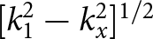 $[k^{2}_{1}-k^{2}_{x}]^{1/2}$. Here, the scattering coefficient
 $C^{L}_{n}$ =
 $C^{TM}_{n}$ for TM polarization and
 $C^{L}_{n}$ =
 $C^{TE}_{n}$ for TE polarization. The term
 $C_{n}$ given by Eq. (24) models all the multiple interactions between the MS-covered cylinder and the flat interface. Likewise, the scattered-reflected field
 $\psi^{s}_{sr}$ in region 0 can be expressed as follows,
 \begin{equation}
\psi^{s}_{sr} = \frac{1}{\pi}\sum_{n=-\infty}^{+\infty}C_{n}^{L}C_{n}I^{L}_{n}
\end{equation}
 \begin{align}
I_{n}^{L} &= \int_{-\infty}^{+\infty}\frac{1}{k_{1y}}T^{L}_{10}(k_{x})e^{j(k_{0y}-k_{1y})d}e^{-j(k_{x}x+k_{0y}y)} \\ \nonumber & \cdot e^{jn\tan^{-1}(k_{1y}/k_{x})}dk_{x}\end{align}
 \begin{equation}
T_{10}^{L}(k_{x}) = \left\{\begin{array}{ll}
\frac{2k_{1y}}{k_{1y}+k_{0y}}, & \textrm{TM polarization}\\
\frac{2k_{0}^{2}k_{1y}}{k_{0}^{2}k_{1y}+k_{1}^{2}k_{0y}}, & \textrm{TE polarization}\\
\end{array} \right.
\end{equation}
The scattered field  $\psi^{s}_{sr}$ in region 0, as given by Eq. (29), can be determined provided that the integral
 $I_{n}^{L}$ is known. We are interested in the SW of an MS-covered cylinder buried below a flat interface. For this, it is desired to find the far-zone scattered field in region 0. This far-zone scattered field in region 0 can be found by solving the integral
 $I_{n}^{L}$ asymptotically using very large values of
 $x$ and
 $y$. This integral
 $I_{n}^{L}$ can be solved using the saddle point integration method [Reference Felsen and Marcuvitz71]. For the saddle point integration method, we will substitute
 $k_{x}$ =
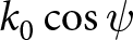 $k_{0}\cos\psi$,
 $x$ =
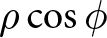 $\rho\cos\phi$,
 $y$ =
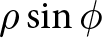 $\rho\sin\phi$ with
 $\rho$ =
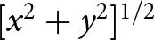 $[x^2+y^2]^{1/2}$ for the integral
 $I_{n}^{L}$. After this, the transformed integral is solved using the saddle point integration method with the saddle point of
 $\psi$ =
 $\phi$. Based on this far-zone scattered field in region 0, the SW can be found using the following definition [Reference Balanis68],
 \begin{equation}
\sigma=\lim_{\rho \rightarrow\infty }2\pi\rho\frac{\mid\psi_{sr}^{s}\mid^{2}}{\mid\psi_{0}^{i}\mid^{2}}
\end{equation}
It should be noted that the total scattered-reflected field  $\psi_{sr}$ in region 0 which is shown in Figure 1 is the sum of
 $\psi^{r}_{0}$ and
 $\psi^{s}_{sr}$ as given by Eqs. (19) and (20), respectively. For the numerical results, we have used normalized SW, i.e.,
 $\sigma_{n}$=
 $\sigma/\lambda_{0}$.
For the special case of a deeply buried MS-covered circular cylinder, we can assume 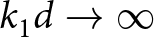 $k_{1}d\rightarrow\infty$ for a fixed value of
 $k_{1}$. In this case, we need to solve the integral
 $I_{m,n}^{L}$ as given by Eq. (27) for the large value of
 $k_{1}d$ asymptotically. Using the saddle point integration method, it can be shown that,
 \begin{equation}
I_{m,n}^{L} = -\sqrt{\frac{\pi}{k_{1}d}}(j)^{m+n}e^{-j(2k_{1}d+\pi/4)}R^{L}
\end{equation}
 \begin{equation}
R^{L} = \left\{\begin{array}{ll}
\frac{k_{1}-k_{0}}{k_{1}+k_{0}}, & \textrm{TM polarization}\\
\frac{k_{0}^{2}k_{1}-k_{1}^{2}k_{0}}{k_{0}^{2}k_{1}+k_{1}^{2}k_{0}}, & \textrm{TE polarization}\\
\end{array} \right.
\end{equation}
Numerical results and discussion
In order to validate the proposed theory, it is assumed that  $Z_{e}$ =
 $Z_{m}$ =
 $\infty$, which corresponds to a circular cylinder without MS. We also assume
 $\epsilon_{r1} = 4-$
 $j$0.01,
 $\epsilon_{r2}$ = 2.25,
 $d$ = 1.3
 $\lambda_{0}$, and
 $\phi_{i}$ = -
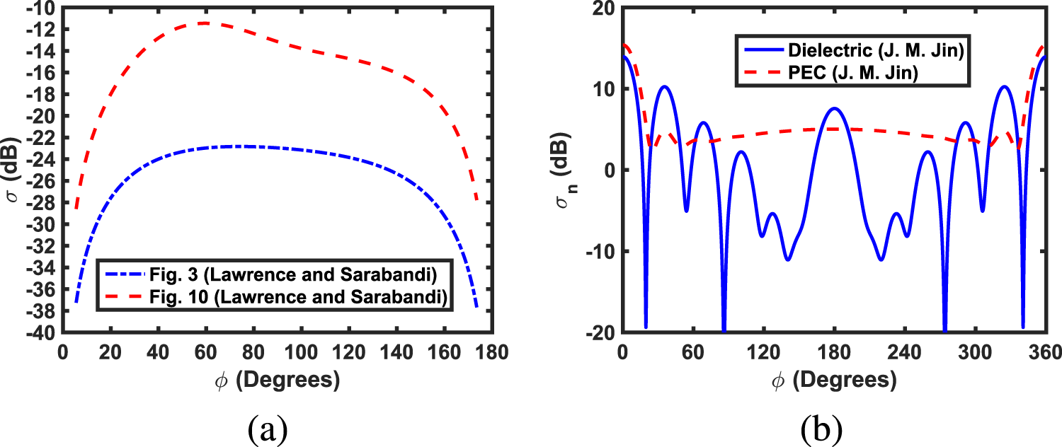
 $60^{\circ}$, as adopted by Lawrence and Sarabandi for TM polarization. It is shown in Figure 2(a) that the reproduced SW results are in excellent agreement with Fig. 3 and Fig. 10 of [Reference Lawrence and Sarabandi24] for
 $a$ = 0.16
 $\lambda_{0}$ and
 $a$ =
 $\lambda_{0}$, respectively. Likewise, if we take depth
 $d$ = 0,
 $a$ =
 $\lambda_{0}$ = 100 mm with
 $\epsilon_{r1}$ =
 $\mu_{r1}$ = 1, i.e., free-space background and
 $Z_{e}$ =
 $Z_{m}$ =
 $\infty$ in the proposed formulation, then this scattering scenario corresponds to a dielectric cylinder with permittivity
 $\epsilon_{r2}$ which is placed in the free-space background. The reproduced normalized SW of this dielectric cylinder with
 $\epsilon_{r2}$ = 4 becomes the same as given by Fig. 6.12(e) of Jin [Reference Jin70] under TM polarization. In the same case as mentioned above, if we take
 $\epsilon_{r2}$ = 1 and
 $Z_{e}$ =
 $Z_{m}$ = 0 instead of
 $\infty$, then this scattering scenario becomes equivalent to scattering from a hollow PEC cylinder placed in the free-space background. Based on the proposed theory, its normalized SW has been shown in Figure 2(b) with a red dashed curve, which is again in excellent agreement with Fig. 6.10(e) of Jin.
(a) Reproduced the SW of a buried dielectric cylinder based on the proposed formulation where all geometrical and electromagnetic parameters have been taken from Lawrence and Sarabandi [Reference Lawrence and Sarabandi24]. (b) Reproduced normalized SWs of dielectric and PEC cylinders based on the proposed theory by taking geometrical and electromagnetic parameters from Jin [Reference Jin70].

Figure 2 Long description
A line graph with the y-axis labeled, sigma, in decibel, ranging from minus 40 to minus 10. The x-axis is labeled, phi, in Degrees, ranging from 0 to 180. Two dashed curves are shown. One curve rises from about minus 30 at 0 degrees to about minus 12 near 60 degrees, then gradually decreases to about minus 16 near 150 degrees and to about minus 28 near 170 degrees. The other curve rises from about minus 40 at 0 degrees to about minus 23 near 60 degrees, stays near minus 23 to minus 24 from about 60 to 120 degrees, then decreases to about minus 28 near 150 degrees and to about minus 38 near 170 degrees. A legend box contains two entries with dashed line samples. The image B showing a line graph with the y-axis labeled, sigma subscript n, in decibel, ranging from minus 20 to 20. The x-axis is labeled, phi, in Degrees, ranging from 0 to 360. Two curves are shown. One curve is a smooth dashed curve that starts near 15 at 0 degrees, drops to about 3 near 30 degrees, stays between about 3 and 6 through most of the range and rises again to near 15 at 360 degrees. The other curve is a solid curve with repeated peaks and deep troughs across 0 to 360 degrees, including several troughs that reach about minus 20 and multiple peaks that reach about 10 to 15. A legend box lists two entries, Dielectric and PEC, each followed by parenthetical text.
To validate the scattering from MM and MS cylinders based on the proposed theory, which are not buried below a flat interface, we assume  $k_{1}$ =
 $k_0$,
 $\eta_{1}$ =
 $\eta_0$, and
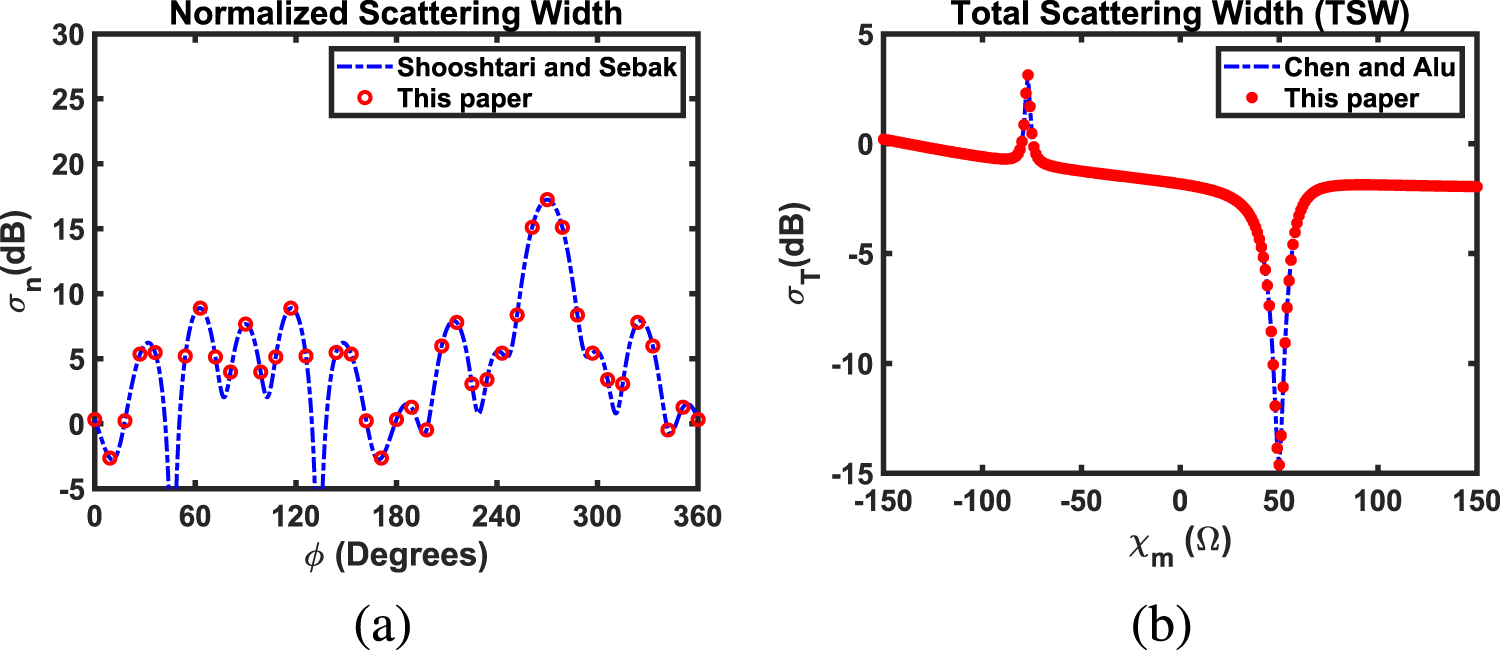
 $d$ = 0 in the proposed formulation. Using this information in the proposed formulation, the normalized SW of a single isolated DNG cylinder with a free-space background has been shown in Figure 3(a), which is in exact agreement with figure 10 of Shooshtari and Sebak [Reference Shooshtari and Sebak72]. In this case, all electromagnetic and geometrical parameters have been taken from [Reference Shooshtari and Sebak72]. To validate the scattering from an MS dielectric cylinder based on the proposed formulation, we have used the definition of total SW (TSW) as given by Chen and Alu [Reference Chen and Alù73]. Using this definition of TSW along with all electromagnetic and geometrical parameters as adopted in [Reference Chen and Alù73], the TSW has been shown in Figure 3(b), which is in excellent agreement with figure 4 of [Reference Chen and Alù73]. These above-mentioned agreements validate the proposed formulations. It should be noted that the operating free-space wavelength
 $\lambda_{0}$ is taken to be 100 mm for all figures except Figures 15 and 16. The truncation index criteria for all the summations appearing in the analytical formulation and the minimum number of interactions between the considered cylindrical object and the flat interface have been adopted from [Reference Akhtar, Naz, Fiaz and Naqvi20, Reference Fiaz21] and references therein.
(a) Normalized SW of an isolated DNG cylinder with the free-space background and (b) the TSW of an MS-covered dielectric cylinder with the free-space background using TM incident polarization.

Figure 3 Long description
Normalized Scattering Width in the image A. Legend entries: Shooshtari and Sebak; This paper. The horizontal axis label is phi, unit Degrees, with values from 0 to 360. The vertical axis label is sigma subscript n, unit decibel, with values from negative 5 to 30. A dashed curve and circular markers are plotted across the full phi range. Total Scattering Width left parenthesis TSW right parenthesis in the image B. Legend entries: Chen and Alu; This paper. The horizontal axis label is X subscript m, unit ohm, with values from negative 150 to 150. The vertical axis label is sigma subscript T, unit decibel, with values from negative 15 to 5. A dashed curve and circular markers are plotted, including a narrow peak near X subscript m around negative 70 and a deep narrow dip near X subscript m around 50.
For all buried MS-covered circular cylinders considered in this section, it is assumed that MS has surface impedance of  $Z^{TM}$ =
 $j\chi_{m}$ and
 $Z^{TE}$ =
 $j\chi_{e}$. Here
 $\chi_{m}$ and
 $\chi_{e}$ represent the surface reactance of an MS, and they can have positive or negative values. For MM circular cylinders, we have assumed
 $\epsilon_{r2} = -2.25$,
 $\mu_{r2}$ = 1 for ENG,
 $\epsilon_{r2}$ = 1,
 $\mu_{r2} = -2.25$ for MNG,
 $\epsilon_{r2}$ =
 $-$2.25,
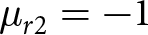 $\mu_{r2} = -1$ for DNG,
 $\epsilon_{r2}$ =
 $10^{-3}$,
 $\mu_{r2}$ = 1 for ENZ [Reference Raqeeb, Awan and Hussain56],
 $\epsilon_{r2}$ = 1,
 $\mu_{r2}$ =
 $10^{-3}$ for MNZ, and
 $\epsilon_{r2}$ =
 $10^{-3}$,
 $\mu_{r2}$ =
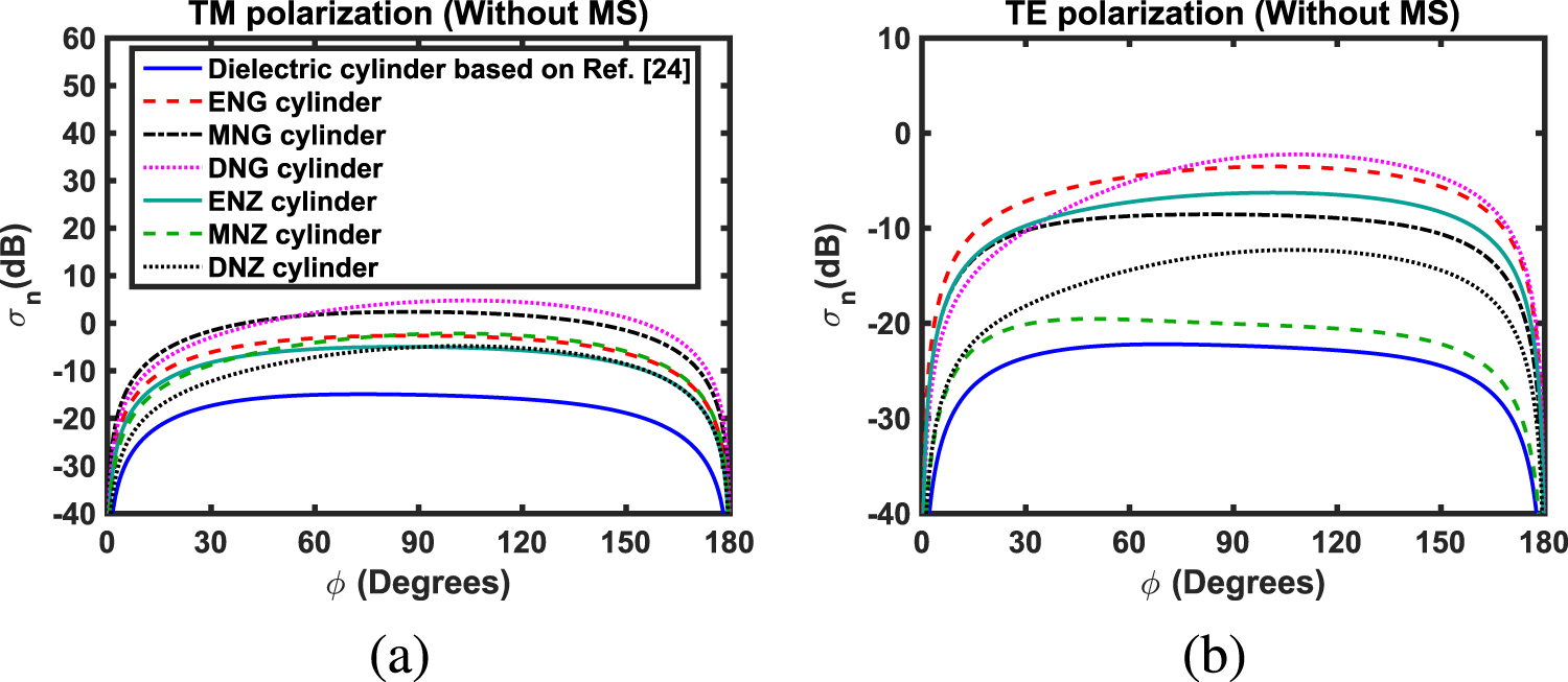
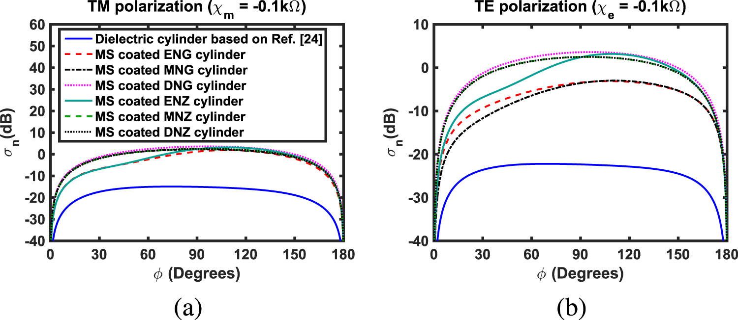
 $10^{-3}$ for DNZ MMs. In order to compare the scattering characteristics of the proposed MS-covered MM cylinders buried below a flat interface with previous work in the literature, we have considered the buried dielectric cylinder as a reference [Reference Lawrence and Sarabandi24]. It should be noted that all electromagnetic and geometrical parameters considered in Figures 4 and 5 are the same as given in [Reference Lawrence and Sarabandi24], except for the electromagnetic parameters of MM cylinders and MS reactances, which are taken to be different. In Figure 4, we have shown the normalized SWs of the considered buried MM cylinders without MS and their comparisons with the normalized SW of a buried dielectric cylinder based on [Reference Lawrence and Sarabandi24]. It is observed from Figure 4 that all the considered buried MM cylinders have enhanced scattering as compared to scattering from a buried dielectric cylinder under both types of incident polarization. Likewise, a comparison between the normalized SWs of buried MS-covered MM cylinders and the normalized SW of a buried dielectric cylinder based on [Reference Lawrence and Sarabandi24] under TM and TE incident polarizations has been shown in Figure 5. For MS, it is assumed that
 $\chi_{m}$ =
 $\chi_{e}$ =
 $-$0.1k
 $\Omega$. Once again, it is found that the considered buried MS-covered MM cylinders have enhanced scattering as compared to scattering from a buried dielectric cylinder. These enhanced scattering characteristics provide interesting results that have not been found in the literature. This study may be helpful in the design of detection systems for buried objects.
Normalized SWs of the buried considered MM cylinders and their comparisons with the normalized SW of a buried dielectric cylinder based on [Reference Lawrence and Sarabandi24] under (a) TM and (b) TE incident polarizations.

Figure 4 Long description
A line graph titled, TM polarization, open parenthesis Without MS close parenthesis. The x-axis label is, phi, open parenthesis Degrees close parenthesis, ranging from 0 to 180 with ticks at 0, 30, 60, 90, 120, 150, 180. The y-axis label is, sigma subscript n, open parenthesis dB close parenthesis, ranging from minus 40 to 60 with ticks at minus 40, minus 30, minus 20, minus 10, 0, 10, 20, 30, 40, 50, 60. The legend lists: Dielectric cylinder based on Ref. link, ENG cylinder, MNG cylinder, DNG cylinder, ENZ cylinder, MNZ cylinder, DNZ cylinder. All curves rise steeply from near minus 40 at phi equals 0, form a broad plateau, then fall steeply back toward minus 40 at phi equals 180. At phi equals 90, the approximate values are: Dielectric cylinder based on Ref. link about minus 15, ENG cylinder about minus 3, MNG cylinder about minus 4, DNG cylinder about plus 4, ENZ cylinder about minus 6, MNZ cylinder about minus 2, DNZ cylinder about minus 6. The image B showing a line graph titled, TE polarization, open parenthesis Without MS close parenthesis. The x-axis label is, phi, open parenthesis Degrees close parenthesis, ranging from 0 to 180 with ticks at 0, 30, 60, 90, 120, 150, 180. The y-axis label is, sigma subscript n, open parenthesis dB close parenthesis, ranging from minus 40 to 10 with ticks at minus 40, minus 30, minus 20, minus 10, 0, 10. The same legend categories are shown. All curves rise steeply from near minus 40 at phi equals 0, form a broad plateau, then fall steeply back toward minus 40 at phi equals 180. At phi equals 90, the approximate values are: Dielectric cylinder based on Ref. link about minus 22, ENG cylinder about minus 4, MNG cylinder about minus 9, DNG cylinder about minus 2, ENZ cylinder about minus 7, MNZ cylinder about minus 20, DNZ cylinder about minus 12.
A comparative study of the normalized SWs of buried MS-covered considered MM cylinders with  $\chi_{m}$ =
 $\chi_{e}$ =
 $-$0.1
 $k\Omega$ and their comparison with the normalized SW of a buried dielectric cylinder based on [Reference Lawrence and Sarabandi24] under (a) TM and (b) TE incident polarizations.

Figure 5 Long description
TM polarization, chi subscript m equals minus 0.1 kilo ohm. The x-axis label is phi, Degrees, ranging from 0 to 180 with ticks at 0, 30, 60, 90, 120, 150, 180. The y-axis label is sigma subscript n, decibel, ranging from minus 40 to 60 with ticks every 10. A legend lists seven curves: Dielectric cylinder based on Ref. [24], MS coated ENG cylinder, MS coated MNG cylinder, MS coated DNG cylinder, MS coated ENZ cylinder, MS coated MNZ cylinder, MS coated DNZ cylinder. The dielectric curve stays below the others, near minus 40 at 0 degrees and 180 degrees and around minus 15 to minus 20 between about 30 and 150 degrees. The six MS coated curves cluster together, near minus 40 at 0 degrees and 180 degrees, rising to around 0 to about 5 between about 60 and 140 degrees, then dropping toward minus 40 near 180 degrees. TE polarization, chi subscript e equals minus 0.1 kilo ohm. The x-axis label is phi, Degrees, ranging from 0 to 180 with ticks at 0, 30, 60, 90, 120, 150, 180. The y-axis label is sigma subscript n, decibel, ranging from minus 40 to 10 with ticks at minus 40, minus 30, minus 20, minus 10, 0, 10. The same seven legend entries appear. The dielectric curve is lowest, near minus 40 at 0 degrees and 180 degrees and around minus 25 to minus 28 between about 30 and 150 degrees. The MS coated curves rise from near minus 40 at 0 degrees to values between about minus 10 and plus 5 around 90 to 120 degrees, then decrease toward minus 40 near 180 degrees.
For Figures 6–16, region 1 is assumed to be a realistic dielectric background medium, which is a low-loss Teflon. This is because it acts as a low-loss material even at relatively higher frequencies. The electromagnetic parameters of the Teflon material are taken to be  $\epsilon_{r1}$ = 2.1
 $-j$0.0002 and
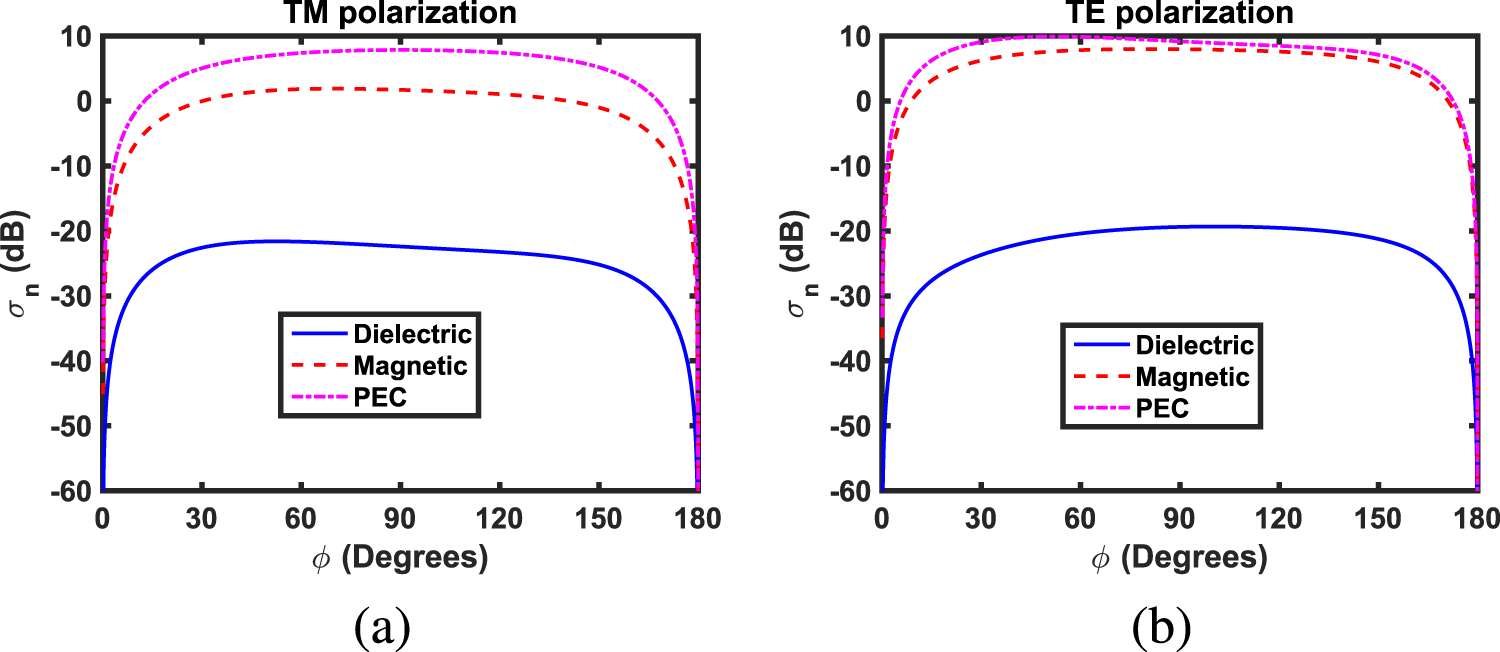
 $\mu_{r1}$ = 1. Likewise, this material is often used as a packaging material for MM circular cylinders. In Figure 6, the normalized SWs of buried dielectric, magnetic, and PEC cylinders without MS have been shown for completeness under both types of incident polarizations. Here
 $\phi_{i}$ =
 $-60^{\circ}$,
 $d$ = 1.5
 $\lambda_{0}$, and
 $a$ = 0.15
 $\lambda_{0}$. It is assumed that
 $\epsilon_{r2}$ = 2.25,
 $\mu_{r2}$ = 1 for a dielectric cylinder and
 $\epsilon_{r2}$ = 1,
 $\mu_{r2}$ = 2.25 for a magnetic cylinder. It is clear from Figure 6 that the SW of the buried PEC cylinder is relatively large as compared to buried dielectric and magnetic cylinders under TM incident polarization. Similar findings have also been observed for the TE polarization. This is because of the reflective nature of the PEC material.
A comparative study of the normalized SWs of buried dielectric, magnetic, and PEC circular cylinders under (a) TM and (b) TE incident polarizations.

The normalized SWs of MS-covered (a) ENG (b) MNG (c) DNG (d) ENZ (e) MNZ, and (f) DNZ circular cylinders buried below a flat interface for TM incident polarization.

Figure 7 Long description
The title, TM polarization, appears above each of six sub images. The image A showing TM polarization, ENG Cylinder. The x axis label is phi, Degrees, ranging from 0 to 180. The y axis label is sigma subscript n, decibel, ranging from minus 40 to 20. A legend lists, Without MS; chi subscript m equals 0.01 kilo ohm; chi subscript m equals 0.1 kilo ohm; chi subscript m equals 1 kilo ohm; chi subscript m equals minus 0.01 kilo ohm; chi subscript m equals minus 0.1 kilo ohm; chi subscript m equals minus 1 kilo ohm. All curves rise from about minus 40 decibel near 0 degrees to a near flat region between about 30 and 150 degrees, then drop back toward about minus 40 decibel near 180 degrees. In the flat region, the curves lie between about 4 and 10 decibel, with the highest curve near about 9 to 10 decibel around 40 to 60 degrees. The image B showing TM polarization, MNG Cylinder. The x axis label is phi, Degrees, ranging from 0 to 180. The y axis label is sigma subscript n, decibel, ranging from minus 20 to 20. The same legend entries appear. Curves rise from about minus 20 decibel near 0 degrees to values around 6 to 9 decibel by about 30 degrees. Between about 40 and 150 degrees, most curves stay between about 5 and 9 decibel, with one curve reaching about 11 to 12 decibel near about 110 to 130 degrees. All curves drop toward about minus 20 decibel near 180 degrees. The image C showing TM polarization, DNG Cylinder. The x axis label is phi, Degrees, ranging from 0 to 180. The y axis label is sigma subscript n, decibel, ranging from minus 20 to 20. The same legend entries appear. Curves rise from about minus 20 decibel near 0 degrees to a broad maximum between about 60 and 140 degrees. The highest curve reaches about 14 to 15 decibel near about 100 to 120 degrees. Several other curves peak around 10 to 13 decibel. All curves fall toward about minus 20 decibel near 180 degrees. The image D showing TM polarization, ENZ Cylinder. The x axis label is phi, Degrees, ranging from 0 to 180. The y axis label is sigma subscript n, decibel, ranging from minus 20 to 20. The same legend entries appear. Most curves rise from about minus 20 decibel near 0 degrees to a plateau around 5 to 8 decibel from about 40 to 150 degrees, then drop toward about minus 20 decibel near 180 degrees. One curve differs by rising to about 9 to 10 decibel near about 30 to 50 degrees, then decreasing to around 0 decibel near about 90 degrees and to about minus 5 decibel near about 150 degrees before dropping near 180 degrees. The image E showing TM polarization, MNZ Cylinder. The x axis label is phi, Degrees, ranging from 0 to 180. The y axis label is sigma subscript n, decibel, ranging from minus 20 to 20. The same legend entries appear. Curves rise from about minus 20 decibel near 0 degrees to a broad peak between about 60 and 140 degrees. The upper curves reach about 8 to 10 decibel near about 90 to 120 degrees. A lower curve peaks near about 0 to 2 decibel around the middle angles. All curves drop toward about minus 20 decibel near 180 degrees. The image F showing TM polarization, DNZ Cylinder. The x axis label is phi, Degrees, ranging from 0 to 180. The y axis label is sigma subscript n, decibel, ranging from minus 20 to 20. The same legend entries appear. Curves rise from about minus 20 decibel near 0 degrees to mid angle values that range from about minus 2 decibel up to about 9 to 10 decibel. The highest curve stays near about 9 to 10 decibel from about 60 to 140 degrees. Several curves lie around 4 to 8 decibel in the same region and one curve remains below 0 decibel for much of the mid angle range. All curves drop toward about minus 20 decibel near 180 degrees.
The normalized SWs of MS-covered (a) ENG (b) MNG (c) DNG (d) ENZ (e) MNZ, and (f) DNZ circular cylinders buried below a flat interface for TE incident polarization.

Figure 8 Long description
TE polarization (ENG Cylinder). The x-axis is labeled, phi (Degrees), with ticks at 0, 30, 60, 90, 120, 150, 180. The y-axis is labeled, sigma n (dB), ranging from minus 30 to 20 with ticks at minus 30, minus 20, minus 10, 0, 10, 20. A legend lists: Without MS; x e equals 0.01k ohm; x e equals 0.1k ohm; x e equals 1k ohm; x e equals minus 0.01k ohm; x e equals minus 0.1k ohm; x e equals minus 1k ohm. All curves rise steeply from near minus 30 at 0 degrees to positive values by about 10 degrees, stay between about 6 and 16 through most of 30 to 160 degrees, then drop sharply toward minus 30 near 180 degrees. TE polarization (MNG Cylinder). The x-axis is labeled, phi (Degrees), with ticks at 0, 30, 60, 90, 120, 150, 180. The y-axis is labeled, sigma n (dB), ranging from minus 20 to 20 with ticks at minus 20, minus 10, 0, 10, 20. Multiple curves closely overlap. They rise from near minus 20 at 0 degrees to around 8 to 10 by about 20 to 40 degrees, remain near about 7 to 10 from about 40 to 150 degrees, then fall steeply toward minus 20 near 180 degrees. TE polarization (DNG Cylinder). The x-axis is labeled, phi (Degrees), with ticks at 0, 30, 60, 90, 120, 150, 180. The y-axis is labeled, sigma n (dB), ranging from minus 20 to 20 with ticks at minus 20, minus 10, 0, 10, 20. Several curves separate widely. One curve reaches about 15 to 17 near 40 to 60 degrees and then declines to about 10 to 12 by about 160 degrees. Another curve rises from near minus 20 at 0 degrees to about 18 near 120 degrees. A dashed curve drops from about 9 near 30 degrees to about 2 to 4 near 120 degrees. All curves drop sharply toward minus 20 near 180 degrees. TE polarization (ENZ Cylinder). The x-axis is labeled, phi (Degrees), with ticks at 0, 30, 60, 90, 120, 150, 180. The y-axis is labeled, sigma n (dB), ranging from minus 20 to 20 with ticks at minus 20, minus 10, 0, 10, 20. Curves rise from near minus 20 at 0 degrees to around 8 to 12 by about 30 to 60 degrees, remain around 7 to 13 through about 60 to 160 degrees, then drop sharply toward minus 20 near 180 degrees. TE polarization (MNZ Cylinder). The x-axis is labeled, phi (Degrees), with ticks at 0, 30, 60, 90, 120, 150, 180. The y-axis is labeled, sigma n (dB), ranging from minus 20 to 20 with ticks at minus 20, minus 10, 0, 10, 20. Curves rise from near minus 20 at 0 degrees to values between about 0 and 12 by about 20 to 40 degrees. Several curves stay near about 7 to 10 from about 40 to 150 degrees. One lower curve stays near about 0 to minus 3 across much of 30 to 150 degrees. All curves drop sharply toward minus 20 near 180 degrees. TE polarization (DNZ Cylinder). The x-axis is labeled, phi (Degrees), with ticks at 0, 30, 60, 90, 120, 150, 180. The y-axis is labeled, sigma n (dB), ranging from minus 20 to 20 with ticks at minus 20, minus 10, 0, 10, 20. Curves rise from near minus 20 at 0 degrees to values between about 5 and 12 by about 20 to 40 degrees. One curve rises more slowly, reaching about 4 to 6 near 120 degrees. Another curve stays near about minus 5 to 0 across about 30 to 150 degrees. All curves drop sharply toward minus 20 near 180 degrees.
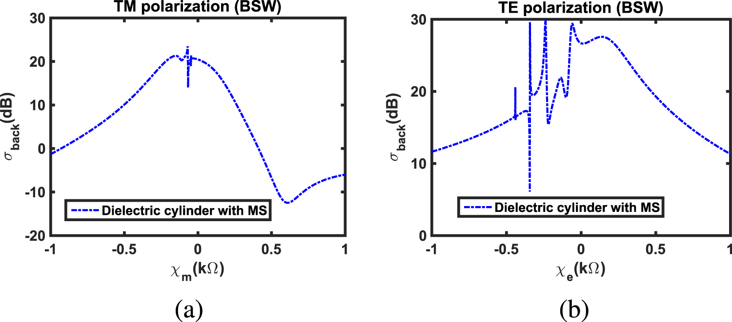
The BSW of a buried MS-covered dielectric cylinder as a function of (a)  $\chi_{m}$ for TM polarization and (b)
 $\chi_{e}$ for TE polarization.

Figure 9 Long description
TM polarization, open parenthesis BSW close parenthesis. The x-axis is labeled, chi subscript m, open parenthesis kilo ohm close parenthesis, with tick labels minus 1, minus 0.5, 0, 0.5, 1. The y-axis is labeled, sigma subscript back, open parenthesis decibel close parenthesis, with tick labels minus 20, minus 10, 0, 10, 20, 30. One dashed curve is shown with legend text, Dielectric cylinder with MS. The curve starts near 0 at chi subscript m equals minus 1, rises to about 10 at minus 0.5, reaches about 21 near chi subscript m around minus 0.1 to 0, then drops to about 20 at 0. It decreases through 10 near about 0.2, crosses 0 near about 0.35, reaches a minimum near minus 12 around chi subscript m about 0.6, then rises to about minus 6 at chi subscript m equals 1. The image B showing TE polarization, open parenthesis BSW close parenthesis. The x-axis is labeled, chi subscript e, open parenthesis kilo ohm close parenthesis, with tick labels minus 1, minus 0.5, 0, 0.5, 1. The y-axis is labeled, sigma subscript back, open parenthesis decibel close parenthesis, with tick labels 0, 10, 20, 30. One dashed curve is shown with legend text, Dielectric cylinder with MS. The curve is near 12 at chi subscript e equals minus 1 and rises to about 16 to 17 near minus 0.5. Between about minus 0.4 and 0, the curve shows several narrow spikes and dips, including a dip near about 6 around chi subscript e about minus 0.35 and peaks reaching about 30 around chi subscript e about minus 0.25 and near about minus 0.05. After 0, the curve stays near about 27 to 28 around chi subscript e about 0.1 to 0.3, then decreases to about 20 near 0.5 and to about 12 at chi subscript e equals 1.
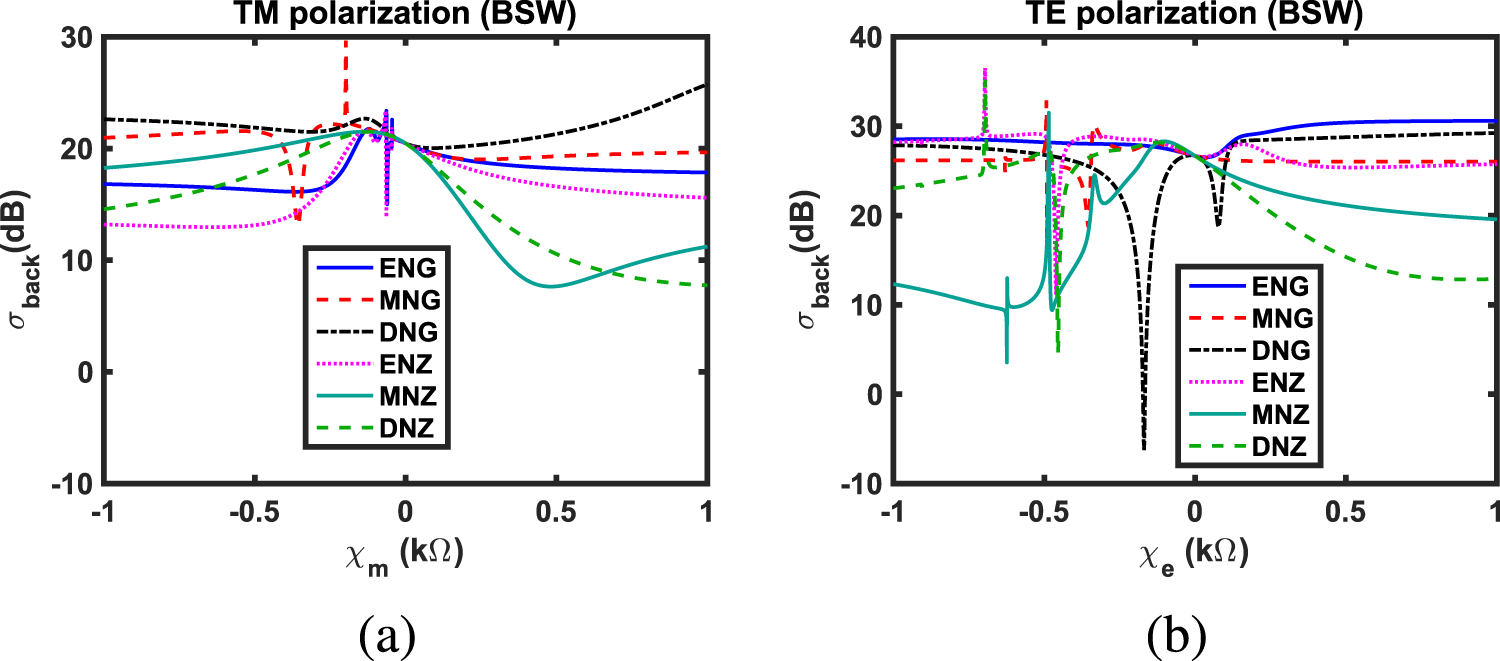
The BSWs of various buried MS-covered MM circular cylinders as a function of (a)  $\chi_{m}$ for TM polarization and (b)
 $\chi_{e}$ for TE polarization.

Figure 10 Long description
TM polarization, BSW. The y-axis label is sigma subscript back, in decibel, ranging from minus 10 to 30. The x-axis label is chi subscript m, in kilo ohm, ranging from minus 1 to 1 with ticks at minus 1, minus 0.5, 0, 0.5 and 1. A legend lists ENG, MNG, DNG, ENZ, MNZ and DNZ. ENG is a solid line that stays near the high teens to low 20s across the range, with a small rise near chi subscript m equals 0. MNG is a dashed line near about 20 to low 20s, with a narrow spike upward near chi subscript m slightly less than 0. DNG is a dash dot line near the low 20s, dipping slightly near chi subscript m around 0 and rising toward the right end. ENZ is a dotted line that rises toward a peak near chi subscript m around 0 and then slopes downward toward the right. MNZ is a solid line that rises toward about the low 20s near chi subscript m around 0, then drops to a trough near chi subscript m around 0.5 and rises again toward the right. DNZ is a dashed line that rises toward the low 20s near chi subscript m around 0, then decreases toward the right side. TE polarization, BSW. The y-axis label is sigma subscript back, in decibel, ranging from minus 10 to 40. The x-axis label is chi subscript e, in kilo ohm, ranging from minus 1 to 1 with ticks at minus 1, minus 0.5, 0, 0.5 and 1. A legend lists ENG, MNG, DNG, ENZ, MNZ and DNZ. ENG is a solid line near the upper 20s, dipping slightly near chi subscript e around 0 and then rising to about 30 toward the right. MNG is a dashed line near the upper 20s with a small dip near chi subscript e around 0 and then stays near the upper 20s. DNG is a dash dot line with a deep narrow dip below 0 near chi subscript e slightly less than 0, then returns to the mid to upper 20s. ENZ is a dotted line near the upper 20s with a small dip near chi subscript e around 0 and then trends slightly downward toward the right. MNZ is a solid line that starts near the low teens at chi subscript e equals minus 1, shows sharp narrow features near chi subscript e around minus 0.6 to minus 0.4, rises to the mid 20s near chi subscript e around 0, then decreases toward about 20 by chi subscript e equals 1. DNZ is a dashed line that is in the mid 20s on the left, then decreases after chi subscript e around 0 toward the low teens by chi subscript e equals 1.
Influences of various radii upon the BSWs of MS-covered (a) ENG (b) MNG (c) DNG (d) ENZ (e) MNZ, and (f) DNZ circular cylinders buried below a flat interface for TM incident polarization.

Figure 11 Long description
TM polarization (ENG cylinder). The x-axis is labeled, chi subscript m (k ohm), with ticks at minus 1, minus 0.5, 0, 0.5, 1. The y-axis is labeled, sigma subscript back (decibel), ranging from 5 to 30 with ticks at 5, 10, 15, 20, 25, 30. A legend lists a equals 0.15 lambda subscript 0, a equals 0.25 lambda subscript 0 and a equals 0.35 lambda subscript 0. The a equals 0.15 lambda subscript 0 curve is a solid line, near 17 at chi subscript m equals minus 1, rises to about 22 near chi subscript m equals 0, then decreases to about 18 by chi subscript m equals 1. The a equals 0.25 lambda subscript 0 curve is dashed, near 20 at chi subscript m equals minus 1, rises to about 23 near chi subscript m equals 0, then is near 21 at chi subscript m equals 1. The a equals 0.35 lambda subscript 0 curve is dash dot, near 22 at chi subscript m equals minus 1, rises to about 24 near chi subscript m equals 0, then is near 23 at chi subscript m equals 1. Narrow vertical spikes are drawn near chi subscript m close to 0. TM polarization (MNG cylinder). The x-axis is labeled, chi subscript m (k ohm), with ticks at minus 1, minus 0.5, 0, 0.5, 1. The y-axis is labeled, sigma subscript back (decibel), ranging from 10 to 30 with ticks at 10, 15, 20, 25, 30. Three curves are shown. One curve has a deep dip to about 13 near chi subscript m around minus 0.35, then rises to about 22 near chi subscript m around minus 0.2 and is near 20 at chi subscript m equals 1. Another curve shows a dip near chi subscript m around minus 0.6 to about 17, then rises to about 24 near chi subscript m around minus 0.3 and is near 24 at chi subscript m equals 1. A third curve is near 27 at chi subscript m equals minus 1, decreases toward about 22 by chi subscript m equals 1. Narrow vertical spikes are drawn near chi subscript m close to 0. TM polarization (DNG cylinder). The x-axis is labeled, chi subscript m (k ohm), with ticks at minus 1, minus 0.5, 0, 0.5, 1. The y-axis is labeled, sigma subscript back (decibel), ranging from 0 to 30 with ticks at 0, 5, 10, 15, 20, 25, 30. Three curves are shown. One curve is near 23 at chi subscript m equals minus 1, stays near 22 to 23 up to chi subscript m near 0, then increases to about 26 at chi subscript m equals 1. Another curve is near 16 at chi subscript m equals minus 1, rises to about 23 near chi subscript m around 0.2, dips to about 16 near chi subscript m around 0.8, then rises again near 21 at chi subscript m equals 1. A third curve is near 10 at chi subscript m equals minus 1, dips to about 5 near chi subscript m around minus 0.2, rises sharply to about 24 near chi subscript m around 0, then decreases toward about 15 by chi subscript m equals 1. Narrow vertical spikes are drawn near chi subscript m close to 0. TM polarization (ENZ cylinder). The x-axis is labeled, chi subscript m (k ohm), with ticks at minus 1, minus 0.5, 0, 0.5, 1. The y-axis is labeled, sigma subscript back (decibel), ranging from 5 to 30 with ticks at 5, 10, 15, 20, 25, 30. Three curves are shown. One curve is near 13 at chi subscript m equals minus 1, rises to about 22 near chi subscript m equals 0, then decreases to about 16 at chi subscript m equals 1. Another curve is near 17 at chi subscript m equals minus 1, rises to about 23 near chi subscript m equals 0, then decreases to about 19 at chi subscript m equals 1. A third curve is near 20 at chi subscript m equals minus 1, rises to about 24 near chi subscript m equals 0, then decreases to about 21 at chi subscript m equals 1. Narrow vertical spikes are drawn near chi subscript m close to 0. TM polarization (MNZ cylinder). The x-axis is labeled, chi subscript m (k ohm), with ticks at minus 1, minus 0.5, 0, 0.5, 1. The y-axis is labeled, sigma subscript back (decibel), ranging from 5 to 25 with ticks at 5, 10, 15, 20, 25. Three curves are shown. One curve is near 18 at chi subscript m equals minus 1, rises to about 21 near chi subscript m around minus 0.2, then drops to about 8 near chi subscript m around 0.5 and rises to about 11 at chi subscript m equals 1. Another curve is near 21 at chi subscript m equals minus 1, rises to about 23 near chi subscript m around minus 0.1, drops to about 13 near chi subscript m around 0.4, then rises to about 17 at chi subscript m equals 1. A third curve is near 22 at chi subscript m equals minus 1, rises to about 24 near chi subscript m around 0, drops to about 16 near chi subscript m around 0.3, then rises to about 20 at chi subscript m equals 1. TM polarization (DNZ cylinder). The x-axis is labeled, chi subscript m (k ohm), with ticks at minus 1, minus 0.5, 0, 0.5, 1. The y-axis is labeled, sigma subscript back (decibel), ranging from 5 to 25 with ticks at 5, 10, 15, 20, 25. Three curves are shown. One curve is near 14 at chi subscript m equals minus 1, rises to about 21 near chi subscript m around minus 0.1, then decreases to about 8 at chi subscript m equals 1. Another curve is near 17 at chi subscript m equals minus 1, rises to about 23 near chi subscript m around minus 0.1, then decreases to about 13 at chi subscript m equals 1. A third curve is near 18 at chi subscript m equals minus 1, rises to about 24 near chi subscript m around minus 0.1, then decreases to about 16 at chi subscript m equals 1.
Effects of various radii upon the BSWs of MS-covered (a) ENG (b) MNG (c) DNG (d) ENZ (e) MNZ, and (f) DNZ circular cylinders buried below a flat interface for TE incident polarization.

Figure 12 Long description
Title text, TE polarization open parenthesis ENG cylinder close parenthesis. The horizontal axis is labeled, chi subscript e open parenthesis k ohm close parenthesis, with tick labels minus 1, minus 0.5, 0, 0.5, 1. The vertical axis is labeled, sigma subscript back open parenthesis decibel close parenthesis, with tick labels 10, 20, 30, 40. A legend lists three curves: a equals 0.15 lambda subscript 0, a equals 0.25 lambda subscript 0 and a equals 0.35 lambda subscript 0. The a equals 0.15 lambda subscript 0 curve stays near 28 to 30, with a dip near chi subscript e around 0. The a equals 0.25 lambda subscript 0 curve is near the low to mid 30s on the left and trends toward about 31 to 32 on the right. The a equals 0.35 lambda subscript 0 curve rises to the high 30s near chi subscript e around minus 0.7, dips to around 29 near chi subscript e around minus 0.1, then increases toward the low 30s. Title text, TE polarization open parenthesis MNG cylinder close parenthesis. The horizontal axis is labeled, chi subscript e open parenthesis k ohm close parenthesis, with tick labels minus 1, minus 0.5, 0, 0.5, 1. The vertical axis is labeled, sigma subscript back open parenthesis decibel close parenthesis, with tick labels 15, 20, 25, 30, 35, 40. Three curves correspond to a equals 0.15 lambda subscript 0, a equals 0.25 lambda subscript 0 and a equals 0.35 lambda subscript 0. The a equals 0.15 lambda subscript 0 curve shows narrow spikes and a deep notch around chi subscript e near minus 0.4, then levels near 26 to 28 toward the right. The a equals 0.25 lambda subscript 0 curve has a sharp dip near chi subscript e around minus 0.3 and a peak near chi subscript e around minus 0.2 reaching the mid 30s, then trends near 29 to 30. The a equals 0.35 lambda subscript 0 curve peaks near chi subscript e around minus 0.2 reaching the high 30s, then settles near about 31. Title text, TE polarization open parenthesis DNG cylinder close parenthesis. The horizontal axis is labeled, chi subscript e open parenthesis k ohm close parenthesis, with tick labels minus 1, minus 0.5, 0, 0.5, 1. The vertical axis is labeled, sigma subscript back open parenthesis decibel close parenthesis, with tick labels minus 10, 0, 10, 20, 30, 40. Three curves correspond to a equals 0.15 lambda subscript 0, a equals 0.25 lambda subscript 0 and a equals 0.35 lambda subscript 0. The a equals 0.15 lambda subscript 0 curve has a very deep narrow minimum near chi subscript e around minus 0.2 reaching below 0, then rises to the high 20s by chi subscript e near 0.5 to 1. The a equals 0.25 lambda subscript 0 curve stays around the mid to high 20s, with a narrow dip near chi subscript e close to 0. The a equals 0.35 lambda subscript 0 curve drops to near the low teens around chi subscript e near minus 0.3, rises to around 30 near chi subscript e near 0, then dips near chi subscript e around 0.2 before trending upward toward the high 20s. Title text, TE polarization open parenthesis ENZ cylinder close parenthesis. The horizontal axis is labeled, chi subscript e open parenthesis k ohm close parenthesis, with tick labels minus 1, minus 0.5, 0, 0.5, 1. The vertical axis is labeled, sigma subscript back open parenthesis decibel close parenthesis, with tick labels 10, 15, 20, 25, 30, 35, 40. Three curves correspond to a equals 0.15 lambda subscript 0, a equals 0.25 lambda subscript 0 and a equals 0.35 lambda subscript 0. The a equals 0.15 lambda subscript 0 curve shows a deep narrow minimum near chi subscript e around minus 0.5 reaching near 10, then stays around the mid 20s to high 20s with a small hump near chi subscript e around 0.2. The a equals 0.25 lambda subscript 0 curve has narrow spikes and dips between chi subscript e around minus 0.6 and minus 0.3, then trends near about 29 to 30. The a equals 0.35 lambda subscript 0 curve peaks near chi subscript e around minus 0.2 reaching the high 30s, then settles near about 31. Title text, TE polarization open parenthesis MNZ cylinder close parenthesis. The horizontal axis is labeled, chi subscript e open parenthesis k ohm close parenthesis, with tick labels minus 1, minus 0.5, 0, 0.5, 1. The vertical axis is labeled, sigma subscript back open parenthesis decibel close parenthesis, with tick labels 0, 5, 10, 15, 20, 25, 30, 35. Three curves correspond to a equals 0.15 lambda subscript 0, a equals 0.25 lambda subscript 0 and a equals 0.35 lambda subscript 0. The a equals 0.15 lambda subscript 0 curve rises from near 10 at chi subscript e near minus 1, shows spikes near chi subscript e around minus 0.6 to minus 0.4, then reaches around the high 20s near chi subscript e around 0 and declines toward about 20 by chi subscript e near 1. The a equals 0.25 lambda subscript 0 curve increases from around 20 at chi subscript e near minus 1, shows sharp dips and peaks between chi subscript e around minus 0.4 and minus 0.2, then trends downward from around 30 near chi subscript e around 0 toward the mid 20s by chi subscript e near 1. The a equals 0.35 lambda subscript 0 curve stays near the mid 20s on the left, shows a sharp dip near chi subscript e around minus 0.2, then rises to around 30 near chi subscript e around 0 and trends near the high 20s. Title text, TE polarization open parenthesis DNZ cylinder close parenthesis. The horizontal axis is labeled, chi subscript e open parenthesis k ohm close parenthesis, with tick labels minus 1, minus 0.5, 0, 0.5, 1. The vertical axis is labeled, sigma subscript back open parenthesis decibel close parenthesis, with tick labels 0, 10, 20, 30, 40. Three curves correspond to a equals 0.15 lambda subscript 0, a equals 0.25 lambda subscript 0 and a equals 0.35 lambda subscript 0. The a equals 0.15 lambda subscript 0 curve has a deep narrow minimum near chi subscript e around minus 0.4 reaching near 5, rises to around the high 20s near chi subscript e around 0, then declines toward the low teens by chi subscript e near 1. The a equals 0.25 lambda subscript 0 curve shows sharp dips and peaks between chi subscript e around minus 0.4 and minus 0.2, then declines from around 30 near chi subscript e around 0 toward about 20 by chi subscript e near 1. The a equals 0.35 lambda subscript 0 curve peaks near chi subscript e around minus 0.2 reaching the high 30s, then declines toward the mid 20s by chi subscript e near 1.
The BSWs of MS-covered (a) ENG (b) MNG (c) DNG (d) ENZ (e) MNZ, and (f) DNZ circular cylinders buried below a flat interface for TM incident polarization for different depths  $d$ = 0.5
 $\lambda_{0}$, 3
 $\lambda_{0}$, and 5
 $\lambda_{0}$.

Figure 13 Long description
A line graph titled, TM polarization ENG cylinder. The x-axis label is chi subscript m, with unit k ohm, with ticks at minus 1, minus 0.5, 0, 0.5, 1. The y-axis label is sigma subscript back, with unit decibel, ranging from 12 to 24 with ticks every 2. A legend lists d equals 0.5 lambda subscript 0, d equals 3 lambda subscript 0 and d equals 5 lambda subscript 0. All three curves are near 17 decibel at chi subscript m equals minus 1, dip slightly near chi subscript m around minus 0.4, then rise to about 22 decibel just left of 0. A narrow vertical spike occurs at chi subscript m equals 0, with the lowest point near 13 decibel and the highest point near 23 decibel. From chi subscript m equals 0 to 1, the curves decrease and end near 18 to 19 decibel. The image B showing a line graph titled, TM polarization MNG cylinder. The x-axis label is chi subscript m, with unit k ohm, with ticks at minus 1, minus 0.5, 0, 0.5, 1. The y-axis label is sigma subscript back, with unit decibel, ranging from 5 to 30 with ticks every 5. The legend lists d equals 0.5 lambda subscript 0, d equals 3 lambda subscript 0 and d equals 5 lambda subscript 0. The curves are near 21 to 22 decibel at chi subscript m equals minus 1, then drop to a deep minimum near chi subscript m around minus 0.35, reaching about 10 decibel for d equals 0.5 lambda subscript 0 and about 7 decibel for d equals 3 lambda subscript 0. A narrow vertical spike is drawn near chi subscript m around minus 0.2, reaching close to 29 decibel. After the spike, the curves are near 22 decibel around chi subscript m equals minus 0.1, then decrease to about 19 to 20 decibel near chi subscript m around 0.2 and rise slightly toward about 20 to 21 decibel at chi subscript m equals 1. The image C showing a line graph titled, TM polarization DNG cylinder. The x-axis label is chi subscript m, with unit k ohm, with ticks at minus 1, minus 0.5, 0, 0.5, 1. The y-axis label is sigma subscript back, with unit decibel, ranging from 10 to 30 with ticks every 5. The legend lists d equals 0.5 lambda subscript 0, d equals 3 lambda subscript 0 and d equals 5 lambda subscript 0. The curves start near 24 decibel at chi subscript m equals minus 1 for d equals 0.5 lambda subscript 0 and near 22 to 23 decibel for the other two. They slope downward toward about 21 to 22 decibel near chi subscript m around minus 0.3, then show a small bump near chi subscript m around minus 0.1 at about 22 decibel. Near chi subscript m equals 0, the curves dip to about 19 to 20 decibel, then rise steadily, reaching about 26 decibel at chi subscript m equals 1. The image D showing a line graph titled, TM polarization ENZ cylinder. The x-axis label is chi subscript m, with unit k ohm, with ticks at minus 1, minus 0.5, 0, 0.5, 1. The y-axis label is sigma subscript back, with unit decibel, ranging from 12 to 24 with ticks every 2. The legend lists d equals 0.5 lambda subscript 0, d equals 3 lambda subscript 0 and d equals 5 lambda subscript 0. The d equals 0.5 lambda subscript 0 and d equals 3 lambda subscript 0 curves start near 13 to 14 decibel at chi subscript m equals minus 1, rise sharply to about 22 decibel just left of 0 and a narrow vertical spike occurs at chi subscript m equals 0 with a low point near 12 decibel and a high point near 23 decibel. The d equals 5 lambda subscript 0 curve is near 17 decibel at chi subscript m equals minus 1 and changes less sharply, staying near 17 to 18 decibel from chi subscript m equals 0 to 1. The other two curves decrease after 0 and end near 16 decibel at chi subscript m equals 1. The image E showing a line graph titled, TM polarization MNZ cylinder. The x-axis label is chi subscript m, with unit k ohm, with ticks at minus 1, minus 0.5, 0, 0.5, 1. The y-axis label is sigma subscript back, with unit decibel, ranging from 5 to 25 with ticks every 5. The legend lists d equals 0.5 lambda subscript 0, d equals 3 lambda subscript 0 and d equals 5 lambda subscript 0. The curves rise from about 18 decibel at chi subscript m equals minus 1 to a broad maximum near chi subscript m around minus 0.1 at about 21 to 22 decibel. They then drop steeply to a minimum near chi subscript m around 0.5 at about 7 to 8 decibel and rise again to about 11 decibel at chi subscript m equals 1. The image F showing a line graph titled, TM polarization DNZ cylinder. The x-axis label is chi subscript m, with unit k ohm, with ticks at minus 1, minus 0.5, 0, 0.5, 1. The y-axis label is sigma subscript back, with unit decibel, ranging from 5 to 25 with ticks every 5. The legend lists d equals 0.5 lambda subscript 0, d equals 3 lambda subscript 0 and d equals 5 lambda subscript 0. The curves rise from about 14 to 15 decibel at chi subscript m equals minus 1 to a peak near chi subscript m around minus 0.1 at about 21 to 22 decibel, then decrease steadily, reaching about 8 decibel at chi subscript m equals 1.
The BSWs of MS-covered (a) ENG (b) MNG (c) DNG (d) ENZ (e) MNZ, and (f) DNZ circular cylinders buried below a flat interface for TE incident polarization at various depths  $d$.

Figure 14 Long description
TE polarization ENG cylinder. The x-axis label is chi subscript e, k ohm, with ticks at minus 1, minus 0.5, 0, 0.5 and 1. The y-axis label is sigma subscript back, decibel, ranging from 5 to 40 with ticks every 5. A legend lists d equals 0.5 lambda subscript 0, d equals 3 lambda subscript 0 and d equals 5 lambda subscript 0. The d equals 0.5 lambda subscript 0 curve is near 28 to 29 from chi subscript e equals minus 1 to about minus 0.2, dips to about 26 to 27 near chi subscript e equals 0, then rises to about 31 to 32 by chi subscript e equals 1. The d equals 3 lambda subscript 0 curve follows a similar path, near 29 at chi subscript e equals minus 1, dipping to about 26 to 27 near 0 and reaching about 31 to 32 at 1. The d equals 5 lambda subscript 0 curve is near 23 to 25 at chi subscript e equals minus 1, shows a narrow peak near chi subscript e around minus 0.6 reaching about 35, then a narrow dip near around minus 0.45 reaching about 10, then rises to about 28 near around minus 0.2 and then decreases toward about 13 by chi subscript e equals 1. The image B showing TE polarization MNG cylinder. The x-axis label is chi subscript e, k ohm, with ticks at minus 1, minus 0.5, 0, 0.5 and 1. The y-axis label is sigma subscript back, decibel, ranging from 15 to 35 with ticks every 5. Three curves are shown. All three are near 26 at chi subscript e equals minus 1. Near chi subscript e around minus 0.5 there is a narrow spike reaching about 33 and a narrow dip reaching about 16. After this region, the curves rise to a broader peak near about 29 to 30 around chi subscript e near minus 0.3, then settle near about 26 by chi subscript e equals 1. The image C showing TE polarization DNG cylinder. The x-axis label is chi subscript e, k ohm, with ticks at minus 1, minus 0.5, 0, 0.5 and 1. The y-axis label is sigma subscript back, decibel, ranging from minus 10 to 30 with ticks every 10. Three curves are shown and largely overlap. Values are near 26 to 28 at chi subscript e equals minus 1. A deep narrow dip occurs slightly left of 0, reaching about minus 5. A second narrower dip occurs slightly right of 0, reaching about 18 to 20. The curves then rise to about 29 to 30 by chi subscript e equals 1. The image D showing TE polarization ENZ cylinder. The x-axis label is chi subscript e, k ohm, with ticks at minus 1, minus 0.5, 0, 0.5 and 1. The y-axis label is sigma subscript back, decibel, ranging from 15 to 40 with ticks every 5. Three curves are shown. Values are near 29 to 30 at chi subscript e equals minus 1. Near chi subscript e around minus 0.5 there is a narrow spike reaching about 37 and a narrow dip reaching about 16. After that, the curves are near 29 around chi subscript e near minus 0.2, then show a shallow dip near chi subscript e around 0.2 to 0.3 reaching about 26 to 27 and end near about 26 at chi subscript e equals 1. The image E showing TE polarization MNZ cylinder. The x-axis label is chi subscript e, k ohm, with ticks at minus 1, minus 0.5, 0, 0.5 and 1. The y-axis label is sigma subscript back, decibel, ranging from 0 to 35 with ticks every 5. Three curves are shown. Two curves start near about 12 at chi subscript e equals minus 1, dip to about 10 near minus 0.7, then show a narrow dip near around minus 0.55 reaching about 3, followed by a sharp rise to about 32 near around minus 0.45. They then drop to about 20 to 22 near around minus 0.3, rise again to about 28 near around minus 0.1 and then decrease gradually to about 19 to 20 by chi subscript e equals 1. The third curve is near about 26 across most of the range, with a narrow spike near around minus 0.45 reaching about 33 and a local rise near around minus 0.35 reaching about 30. The image F showing TE polarization DNZ cylinder. The x-axis label is chi subscript e, k ohm, with ticks at minus 1, minus 0.5, 0, 0.5 and 1. The y-axis label is sigma subscript back, decibel, ranging from minus 20 to 40 with ticks every 10. Three curves are shown and largely overlap. Values are near about 23 to 25 at chi subscript e equals minus 1. Near chi subscript e around minus 0.5 there is a narrow spike reaching about 35 and a deep narrow dip reaching about minus 18. The curves then rise to about 27 to 28 near chi subscript e around 0 and then decrease to about 12 to 13 by chi subscript e equals 1.
The BSWs of an MS-covered frequency-dispersive DNG circular cylinder buried below a flat interface for (a) TM polarization and (b) TE polarization for various values of cylinder radii  $a$ and MS reactances. Here, depth
 $d$ of the cylinder is fixed at 1.5
 $\lambda_{0}$.

Figure 15 Long description
The left heatmap is titled sigma back open parenthesis TM close parenthesis. The vertical axis is labeled Radius over wavelength, ranging from 0.15 to 0.35. The horizontal axis is labeled Xm open parenthesis k subscript 0 close parenthesis, ranging from minus 1.0 to 1.0. The color gradient from blue to red represents increasing sigma back values. The maximum value is marked near Xm equals minus 0.6 and Radius equals 0.30. The right heatmap is titled sigma back open parenthesis TE close parenthesis. The vertical axis is labeled Radius over wavelength, ranging from 0.15 to 0.35. The horizontal axis is labeled Xc open parenthesis k subscript 0 close parenthesis, ranging from minus 1.0 to 1.0. The color gradient from blue to red represents increasing sigma back values. The maximum value is marked near Xc equals minus 0.4 and Radius equals 0.25. The color bar on the right side of each heatmap indicates the sigma back values, with blue representing lower values and red representing higher values. The TM polarization shows a more dispersed maximum compared to the TE polarization, which has a concentrated maximum area.
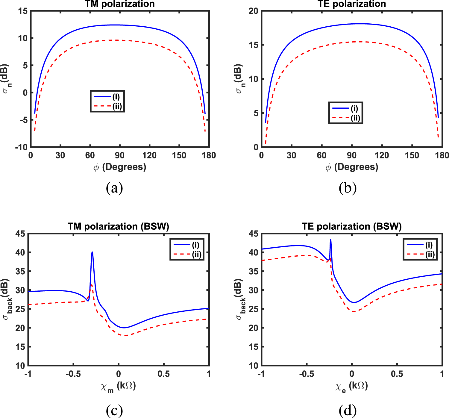
Here, case (i) corresponds to a case where  $d$ = 1.5
 $\lambda_{0}$, and case (ii) corresponds to a deeply buried MS-covered frequency-dispersive DNG circular cylinder. The normalized SW for cases (i) and (ii) for (a) TM polarization and (b) TE polarization with
 $\chi_{m}$ =
 $\chi_{e}$ = 1k
 $\Omega$. The BSWs for cases (i) and (ii) for (c) various values of
 $\chi_{m}$ with TM polarization and (d) various values of
 $\chi_{e}$ with TE polarization. Here,
 $a$ is fixed, i.e.,
 $a$ = 0.15
 $\lambda_{0}$.

Figure 16 Long description
The line graph titled, TM polarization. The horizontal axis is labeled, phi (Degrees), with tick labels 0, 30, 60, 90, 120, 150, 180. The vertical axis is labeled, sigma subscript n (dB), with tick labels minus 10, minus 5, 0, 5, 10, 15. A legend shows two series: (i) as a solid line and (ii) as a dashed line. The solid line rises from about minus 5 at phi equals 0 to about 12 near phi equals 90, then falls to about minus 5 at phi equals 180. The dashed line rises from about minus 7 at phi equals 0 to about 10 near phi equals 90, then falls to about minus 7 at phi equals 180. The line graph titled, TE polarization. The horizontal axis is labeled, phi (Degrees), with tick labels 0, 30, 60, 90, 120, 150, 180. The vertical axis is labeled, sigma subscript n (dB), with tick labels 0, 5, 10, 15, 20. A legend shows two series: (i) as a solid line and (ii) as a dashed line. The solid line rises from about 0 at phi equals 0 to about 18 near phi equals 90, then falls to about 0 at phi equals 180. The dashed line rises from about 0 at phi equals 0 to about 15 near phi equals 90, then falls to about 0 at phi equals 180. The line graph titled, TM polarization (BSW). The horizontal axis is labeled, chi subscript m (k ohm), with tick labels minus 1, minus 0.5, 0, 0.5, 1. The vertical axis is labeled, sigma subscript back (dB), with tick labels 10, 15, 20, 25, 30, 35, 40, 45. A legend shows two series: (i) as a solid line and (ii) as a dashed line. The solid line is near 30 at chi subscript m equals minus 1, stays near 30 up to around chi subscript m equals minus 0.4, then peaks near 40 around chi subscript m equals minus 0.3, drops to about 20 near chi subscript m equals 0 and rises to about 25 at chi subscript m equals 1. The dashed line is near 26 at chi subscript m equals minus 1, rises to about 27 near chi subscript m equals minus 0.4, peaks near 31 around chi subscript m equals minus 0.3, drops to about 18 near chi subscript m equals 0 and rises to about 22 at chi subscript m equals 1. The line graph titled, TE polarization (BSW). The horizontal axis is labeled, chi subscript e (k ohm), with tick labels minus 1, minus 0.5, 0, 0.5, 1. The vertical axis is labeled, sigma subscript back (dB), with tick labels 10, 15, 20, 25, 30, 35, 40, 45. A legend shows two series: (i) as a solid line and (ii) as a dashed line. The solid line is near 41 at chi subscript e equals minus 1, rises to about 42 near chi subscript e equals minus 0.6, shows a narrow peak near 43 around chi subscript e equals minus 0.3, drops to about 27 near chi subscript e equals 0 and rises to about 35 at chi subscript e equals 1. The dashed line is near 38 at chi subscript e equals minus 1, rises to about 39 near chi subscript e equals minus 0.6, drops to about 24 near chi subscript e equals 0 and rises to about 32 at chi subscript e equals 1.
In Figures 7 and 8, the influences of various surface reactances  $\chi_{m}$ and
 $\chi_{e}$ upon the normalized SWs of MS-covered buried MM cylinders have been shown. In these figures, both types of incident polarizations have been considered. For completeness, these SWs have also been compared with the SWs of buried MM circular cylinders without MS. Here
 $\phi_{i}$ = -
 $60^{\circ}$,
 $d$ = 1.5
 $\lambda_{0}$, and
 $a$ = 0.15
 $\lambda_{0}$. In the case of TM polarization, as shown in Figure 7, it is found that the SWs of inductive MS-covered ENG and ENZ circular cylinders are greater than their corresponding SWs of ENG and ENZ circular cylinders without MS, where for inductive MS, we have assumed
 $\chi_{m}$ = 0.01, 0.1, and 1 k
 $\Omega$. It is also observed that an ENZ cylinder covered with
 $\chi_{m}$ =
 $-$0.1k
 $\Omega$ gives asymmetrical scattering as compared to scattering from an ENZ cylinder without MS. It is further studied that the capacitive MS can be used to enhance the SW of a DNZ circular cylinder, where, for capacitive MS, we have adopted
 $\chi_{m}$ =
 $-$0.01,
 $-$0.1, and
 $-$1 k
 $\Omega$. For TE polarization, which is shown in Figure 8, it is found that all the SWs of MS-covered MNG circular cylinders are almost identical for the considered capacitive and inductive values of
 $\chi_{e}$, except
 $\chi_{e}$ =
 $-$0.1k
 $\Omega$. In the case of an MNZ circular cylinder, it is argued that the inductive MS with
 $\chi_{e}$ = 0.01, 0.1, and 1 k
 $\Omega$ can be used to enhance the SW as compared to the SW of an MNZ cylinder without MS. For the DNZ circular cylinder, it is argued that the use of capacitive MS with
 $\chi_{e}$ =
 $-$0.01,
 $-$0.1, and
 $-$1 k
 $\Omega$ can enhance the SW. In the case of an MS-covered DNG cylinder, specific MSs with
 $\chi_{e}$ =
 $\pm$0.01 k
 $\Omega$,
 $\chi_{e}$ =
 $\pm$0.1 k
 $\Omega$ can be used to reduce the SW as compared to the SW of a DNG cylinder without MS.
In the case of scattering from buried cylindrical targets, we are mainly interested in backscattering, which is the measure of how effectively a cylindrical target scatters incoming radiation towards its source. This study of backscattering is important in the design of optical and microwave detection systems, which play a vital role in military systems, civilian systems, avionics, navigation safety, and remote sensing [Reference Awan and Seetharamdoo74]. In the present work, for the backscattering width (BSW), i.e.,  $\sigma_{back}$, we take
 $\phi$ =
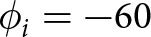 $\phi_{i} = -60$
 $^{\circ}$ in the definition of the normalized SW
 $\sigma_{n}$. These BSWs have been considered in Figures 9–15 and Figure 16(c) and (d). In Table 1, the BSWs of buried dielectric and all considered buried MM circular cylinders without MS have been tabulated for both types of incident polarization. Here
 $a$ = 0.15
 $\lambda_{0}$,
 $d$ = 1.5
 $\lambda_{0}$,
 $\epsilon_{r1}$ = 2.1
 $-j$0.0002,
 $\mu_{r1}$ = 1,
 $\phi$ =
 $\phi_{i}$ =
 $-$60
 $^{\circ}$. It should be noted that these considered geometrical and electromagnetic parameters are slightly different from those considered in [Reference Lawrence and Sarabandi24]. But for a buried dielectric cylinder, we have assumed
 $\epsilon_{r2}$ = 2.25,
 $\mu_{r2}$ = 1 as given in [Reference Lawrence and Sarabandi24]. It is found that a significant enhancement in the backscattering is observed in the case of all considered buried MM cylinders as compared to the backscattering from a buried dielectric cylinder. It is also observed that the minimum value of BSW is observed for a buried DNZ cylinder under TM incidence, and the maximum value of BSW is found for a buried DNG cylinder under TE incidence.
Comparative study of BSWs of dielectric and various MM circular cylinders without MS and buried below a flat interface. All the table entries of  $\sigma_{back}$ have been expressed in dBs

Table 1 Long description
Backscattering width values in decibels are listed for types of cylinders under two columns, TM polarization and TE polarization. Dielectric, Ref. 24, is minus 8.5927 for TM and minus 3.5810 for TE. ENG is 17.3755 for TM and 30.6772 for TE, and MNG is 20.0671 for TM and 26.0899 for TE. ENZ is 14.3293 for TM and 26.8715 for TE, DNZ is 10.0273 for TM and 17.8217 for TE, and MNZ is 15.4920 for TM and 17.0017 for TE. Across the metamaterial rows, TE values are higher than TM values for every type listed.
In order to highlight the impact of various surface reactances upon these considered dielectric and MM circular cylinders, the effects of various  $\chi_{m}$ and
 $\chi_{e}$ upon the BSWs of buried dielectric and considered buried MM cylinders have been shown in Figures 9 and 10. As a general remark, it can be seen from Figures 9 and 10 that by varying the reactances
 $\chi_{m}$ and
 $\chi_{e}$, the BSWs of MS-covered dielectric and MM cylinders can be enhanced or diminished as compared to their respective BSWs of dielectric and MM cylinders without MS under both types of incident polarizations. Various peaks associated with the BSW are apparent in these figures for the specific values of
 $\chi_{m}$ and
 $\chi_{e}$. These resonant peaks arise due to constructive interaction of the backscattered field of the outer cylindrical MS and the backscattered field of the considered dielectric or MM cylinders without MS. Similar reasoning exists for resonant peaks which appear in Figures 11–14. Two optimum cases can be highlighted based on Figure 10 and are relevant to TE incident polarization. In the first case, it is observed that a significant enhancement of 17.3 dB in BSW occurs for the MS-covered DNZ cylinder with
 $\chi_{e}$ =
 $-$696
 $\Omega$ as compared to the BSW of the same DNZ cylinder without MS. In the second case, it is shown that the MS with
 $\chi_{e}$ =
 $-$169
 $\Omega$ can be used to significantly reduce the BSW of a DNG cylinder. This reduction in the BSW is found to be 39.6 dB. Thus, it is concluded that the specific types of MSs can be used to significantly enhance and diminish the BSW of buried DNZ and DNG circular cylinders, respectively.
Influences of various MM circular cylinder radii on the BSWs of MS-covered MM circular cylinders buried below a flat interface have been shown in Figures 11–12 under TM and TE incident polarization. In this case, the depth of all cylinders is taken to be fixed, i.e.,  $d$ = 1.5
 $\lambda_{0}$. In the case of TM polarization, it is observed from Figure 11 that the maximum value of
 $\sigma_{back}\approx$ 29.75 dB is found for ENG and ENZ cylinders, both having the same radii of
 $a$ = 0.25
 $\lambda_{0}$ but different values of
 $\chi_{m}$. For an ENG cylinder, we have
 $\chi_{m} = -80$
 $\Omega$, and for an ENZ cylinder, we have
 $\chi_{m}$ =
 $-$87
 $\Omega$. Thus, it can be concluded that two different MM cylinders, i.e., ENG and ENZ cylinders having the same size with different values of
 $\chi_{m}$, can have the same backscattering characteristics. This type of similar backscattering characteristics with different MMs and MSs may find applications in optical or electromagnetic illusions. On the other hand, the minimum value of
 $\sigma_{back}$ = 4.26 dB is found for the DNG cylinder with a radius of 0.35
 $\lambda_{0}$ and covered with the MS having
 $\chi_{m}$ =
 $-$167
 $\Omega$. In the case of TE polarization, it is seen from Figure 12 that the maximum value of
 $\sigma_{back}$ = 38.41 dB, which is observed for the MS-covered ENZ cylinder with a radius of 0.35
 $\lambda_{0}$ having
 $\chi_{e}$ =
 $-$266
 $\Omega$. Likewise, the minimum value of backscattering is equal to
 $-$6.25 dB, which is found for the MS-covered DNG cylinder having radius
 $a$ = 0.15
 $\lambda_{0}$ with
 $\chi_{e}$ =
 $-$169
 $\Omega$.
In Figures 13–14, the BSWs of various considered MS-covered MM circular cylinders as a function of various MS surface reactances have been shown with different values of  $d$. In this case, we have assumed
 $a$ = 0.15
 $\lambda_{0}$ and
 $d$ = 0.5
 $\lambda_{0}$, 3
 $\lambda_{0}$, and 5
 $\lambda_{0}$. As the value of
 $d$ lies within a few wavelengths, there is no significant change in BSW of the various considered MS-covered MM circular cylinders due to the increasing value of
 $d$ except in some cases, which are shown in Figure 14(a) and (e). In these sub-figures, rapid fluctuations in BSWs are observed for
 $d$ = 5
 $\lambda_{0}$ as compared to their respective BSWs for
 $d$ = 0.5
 $\lambda_{0}$, 3
 $\lambda_{0}$.
In the previous analysis, all considered MM circular cylinders were assumed to be lossless, but in fact, these MMs are inherently lossy and frequency-dispersive [Reference Ziolkowski and Heyman75, Reference Smith, Schultz, Markos and Soukoulis76]. Therefore, in order to incorporate the effects of losses in these MM circular cylinders, we have considered only DNG cylinders. The frequency-dispersive relative permittivity  $\epsilon_{r2}(\omega)$ and relative permeability
 $\mu_{r2}(\omega)$ of such a DNG cylinder is described by the following equations,
 \begin{equation}
\epsilon_{r2}(\omega) = 1 - \frac{\omega^{2}_{pe}}{\omega^{2}-\omega^{2}_{oe}+i\Gamma_{e}\omega}
\end{equation}
 \begin{equation}
\mu_{r2}(\omega) = 1 - \frac{\omega^{2}_{pm}}{\omega^{2}-\omega^{2}_{om}+i\Gamma_{m}\omega}
\end{equation}
Here we have assumed 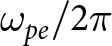 $\omega_{pe}/2\pi$ = 3.2 GHz,
 $\omega_{pm}/2\pi$ = 3.3 GHz,
 $\omega_{oe}/2\pi$ = 8.4 GHz,
 $\omega_{om}/2\pi$ = 8.5 GHz with
 $\Gamma_{e}$ =
 $\Gamma_{m}$ = 0.2 GHz [Reference Ziolkowski and Heyman75, Reference Smith, Schultz, Markos and Soukoulis76]. Using an operating frequency of
 $\omega/2\pi$ = 8.557 GHz, it is found that
 $\epsilon_{r2}$ =
 $-$1.72166
 $-j$1.74959 and
 $\mu_{r2}$ =
 $-$1.73293
 $- j$4.81063, which shows that the real parts of relative permittivity and relative permeability are almost equal. These above-mentioned values of
 $\epsilon_{r2}$ and
 $\mu_{r2}$ for the DNG circular cylinder have been used in Figures 15 and 16.
The influence of various values of surface reactances, i.e.,  $\chi_{m}$,
 $\chi_{e}$, and various radii of frequency-dispersive DNG circular cylinders upon the BSWs has been shown in Figure 15 for both types of incident polarization. In this figure, the region where the BSWs can be significantly enhanced for specific values of
 $\chi_{m}$,
 $\chi_{e}$, and radii
 $a$ is clearly pointed out. These types of buried circular cylinders may be used in the design of optical or microwave detection systems. In Figure 16, the radii of frequency-dispersive DNG circular cylinders are taken to be
 $a$ = 0.15
 $\lambda_{0}$. For case (i), the depth of the considered circular cylinder is fixed at
 $d$ = 1.5
 $\lambda_{0}$, whereas for case (ii), the considered circular cylinder is deeply buried with
 $d$ = 100
 $\lambda_{0}$. Figure 16(a) and (b) presents the normalized SW for cases (i) and (ii) under both types of incident polarization. It is observed that for deeply buried objects, the normalized SWs for both polarizations are reduced. This is because of the weak interaction of deeply buried objects with a flat interface, which in turn reduces the overall scattering. The BSWs as a function of
 $\chi_{m}$,
 $\chi_{e}$ have been shown in Figure 16(c) and (d) for both types of incident polarization. It is again shown that for a deeply buried case (ii), the BSWs are smaller for almost all the considered range of
 $\chi_{m}$,
 $\chi_{e}$ as compared to the corresponding BSWs of case (i).
Conclusions
The scattering properties of an MS-covered MM cylinder buried below a flat interface have been studied. The upper medium of a flat interface is taken to be free space, whereas the lower medium is a dielectric medium. The types of MMs considered for buried circular cylinders are ENG, MNG, double negative, ENZ, MNZ, and DNZ. Spectral plane-wave representation of fields has been used to study the multiple interactions between MS-covered circular cylinders and a flat interface. Analytical expressions of the scattering coefficients of an MS-covered circular cylinder have been derived by applying the double-sided impedance boundary conditions at the cylindrical surface of the considered circular cylinder. The influences of various lossless MS surface reactances, radii, and depths of MS-covered MM circular cylinders upon the normalized SW have been explored. It is shown that by varying surface reactances of the MS, the SW can be enhanced and diminished for the considered buried MM circular cylinders. Later on, we concentrated on backscattering characteristics. Two interesting results were observed during the study for TE incident polarization. In the first case, it is shown that a significant enhancement of nearly 17 dB occurs in the BSW of the buried MS-covered DNZ MM circular cylinder with a surface reactance of  $-$696
 $\Omega$ as compared to the BSW of the same buried DNZ circular cylinder without MS. In the second case, it is shown that the use of an MS with a surface reactance of
 $-$169
 $\Omega$ can significantly reduce the BSW of nearly 39 dB of a buried double-negative MM circular cylinder. It is also shown that the buried MS-covered ENG and ENZ MM circular cylinders of the same size but with different values of MS capacitive reactance have the same backscattering characteristics under the incident TM polarization. These above-mentioned findings may have practical applications in the design of microwave or optical detection systems, stealth systems, and illusion systems.
Funding Statement
This research received no specific grant from any funding agency, commercial or not-for-profit sectors.
Competing interests
The authors report no conflict of interest.

Zeeshan Akbar Awan received the Master of Philosophy from the Department of Electronics, Quaid-i-Azam University, Islamabad, Pakistan in 2002. He has completed his PhD degree in Electronics from the same university. He worked in the Instrumentation and Measurement Group (GIM), Institute of Telecommunications, Lisbon, Portugal, in 2009. He worked as a postdoctoral candidate within the LEOST Laboratory of the COSYS department in IFSTTAR, Lille, France, from January to July 2018. He is presently a professor at the Department of Electronics, Quaid-i-Azam University, Islamabad, Pakistan. He has authored or co-authored more than 40 research articles. His research interests include electromagnetic scattering, MMs, metasurfaces, and antenna theory.

Shahida Zeb received her Master’s degree in Electronics from Quaid-i-Azam University, Islamabad, Pakistan in 2014. She has also received her Master of Philosophy degree in Electronics from the same university in 2019. Currently, she is pursuing her PhD degree in the field of electromagnetic scattering from the same university. Her research interests include electromagnetic scattering from buried objects made up of MM and graphene.

Saba Rahim received her BS degree in Physics with her thesis in the field of nanotechnology from International Islamic University, Islamabad, Pakistan, in 2018. She received her Master of Philosophy degree in Electronics from the Quaid-i-Azam University, Islamabad, Pakistan in 2024. Her main areas of research include electromagnetic scattering from buried targets and MMs.

Arshad Hussain is an Associate Professor at the Department of Electronics, Quaid-i-Azam University (QAU), Islamabad, Pakistan. He is a member of IEEE and a registered engineer with the Pakistan Engineering Council (PEC). He has more than 20 years of experience in research and education at the international as well as national level. He also worked as a research assistant for one year before his PhD at the Austrian Academy of Sciences, Austria. He holds his doctorate in Microelectronics from the State Key Laboratory of Analog and Mixed-Signal VLSI Laboratory, University of Macau, Macau, China. He has worked as a postdoctoral candidate for one year at Chosun University, Gwangju, South Korea. His area of expertise is analog and mixed-signal IC design, with a special focus on circuit design techniques in nanometer CMOS for data conversion techniques. He has developed a System-on-Chip (SoC) Design Laboratory to facilitate IC design research. He has been actively contributing to academic development by introducing a new curriculum on IC design. He is serving as a reviewer for several international IEEE journals and conferences. He organized the International Annual Innovation Summit for Microelectronics and Artificial Intelligence (AI) three times in collaboration with IRP at the Department of Electronics, QAU.