1. Introduction
This paper explores the interesting question of how people’s behavioral attributes, in terms of their decisions regarding how much to consume in current and future periods (in other words, their rate of time preference—RTP hereafter—or their degree of impatience), along with environmental externalities, measured by the production damages associated with polluting emissions, jointly impact upon economic development and the growth prospects of a nation. Specifically, we analyze a stylized endogenous growth setting in which the production process takes place via an AK technology (Rebelo, Reference Rebelo1991; Bretschger and Smulders, Reference Bretschger and Smulders2007) but also generates emissions which pollute the environment (Stokey, Reference Stokey1998; Jouvet et al., Reference Jouvet, Michel and Rotillon2005), while public abatement aims at reducing such pollution (Smulders and Gradus, Reference Smulders and Gradus1996; Liddle, Reference Liddle2001). We characterize how the long-term developmental pattern, which may alternatively take the form of a stagnation or a growth regime, is affected by environmental externalities, exploring how public policy may purposefully be employed to improve the outcome.
Our paper thereby integrates two important issues, the impact of people’s behavioral attributes and the effects of environmental externalities, which together contribute to shaping the prospects of economic development. The first deals with the role of time preference in shaping a country’s path towards a particular developmental regime, while the second, with how the implications of cross-country heterogeneity in environmental damages could lead some countries to suffer more than others from the consequences of climate change. By analyzing how these issues are mutually related, we show that differences in environmental damages may explain why some countries may be doomed to stagnation with the unlikely possibility of emerging from it while others may experience growth and achieve sustained improvements in living standards. This suggests that the effects of climate change on economic development are more important than currently believed, as global warming could widen the gap between the rich and poor regions of the world even further (Dennig et al., Reference Dennig, Budolfson, Fleurbaey, Siebert and Socolow2015; Taconet et al., Reference Taconet, Mejean and Guivarch2020). Indeed, among the countries that are deemed as most vulnerable to climate change, there are some of the poorest countries in the world, such as sub-Saharan Africa, in which resources and possibly efforts to effectively implement damage mitigation measures might be insufficient or unsuccessfully wasted (UNEP, 2001; IPCC, 2022). In this context, our paper shows that if there is a commitment to increase spending on mitigation (in the form of emissions abatement) and taxes are levied optimally for that purpose, then an economy may escape stagnation and pursue a path of sustained growth, suggesting that policy actions may play an essential role in fighting the adverse effects of climate change.
A key feature of our work is that the RTP is not constant, although the constancy of RTP is often considered standard in the literature. However, several studies stress the need to relax this assumption due to empirical observations and growing sustainability considerations. Indeed, empirical evidence shows that the dynamics of savings and returns on savings as determined by financial markets are consistent with an RTP declining over time (Harvey, Reference Harvey1994; Laibson, Reference Laibson1997). Moreover, since climate mitigation policy varies over time so does the extent of environmental degradation and damages, yielding an endogenous change in the relative importance of present and future outcomes and so in the RTP (Weitzman, Reference Weitzman1994; Stern, Reference Stern2022).Footnote 1 Building on these considerations, we assume that the RTP varies with the stock of wealth, and in particular it is a decreasing function of capital, such that an increase in the latter leads to more patience, more capital accumulation and prosperity in a high-growth equilibrium (Strulik, Reference Strulik2012).Footnote 2 As economic activities generate polluting emissions which reduce production capabilities through a damage function, environmental externalities deter capital accumulation and thus reduce patience and prosperity. This tension between economic growth and environmental degradation drives the dynamic evolution of the RTP and the whole process of economic development.
The presence of such an environmental damage which generates a negative production externality implies that from a normative perspective it may be optimal to reduce pollution even if preferences are independent from environmental outcomes. Therefore, different from other studies in which environmental preferences drive policy interventions (John and Pecchenino, Reference John and Pecchenino1994; Chu et al., Reference Chu, Lai and Liao2016), in our setup the utility function depends only on consumption and thus environmental considerations justify the introduction of green policies only through their indirect effects on consumption (Nordhaus and Jorgenson, Reference Nordhaus2013; Ansuategi and Marsiglio, Reference Ansuategi and Marsiglio2017). Note that such indirect effects take place through two different channels related to the changes that abatement generates on production capabilities and the capital stock, determining the level of resource availability and the degree of impatience, respectively.
By balancing the short and long run economic-environmental trade off, a utilitarian government needs to choose an optimal income tax rate (in both a growth- and a welfare-maximizing sense) to finance publicly provided abatement (Ligthart and van der Ploeg, Reference Ligthart and van der Ploeg1994; Ghosh et al., Reference Ghosh, Ray Barman and Gupta2020). Although the environment does not directly affect either the utility function or the RTP, it is environmental parameters (i.e., the elasticity of damages and the elasticity of pollution with respect to unabated emissions) that drive the optimal tax rate, which in turn determines which of the two alternative regimes an economy ends up in: one leading to stagnation and another to sustained growth. Importantly, the existence of these two regimes is a consequence of the RTP being determined by the accumulated stock of capital, which in turn affects and is affected by environmental outcomes and thus by the optimal choice of the tax rate.
Our results show that an increase in the propensity of emissions to damage the environment (i.e., the elasticity of environmental damages) will reduce output and therefore encourage an optimizing government to raise the income tax rate to finance abatement spending. This in turn will have two contrasting effects on economic growth. On the one hand, the reduction in disposable income will reduce capital accumulation and growth, resulting in an increase in the degree of impatience and hence in consumption. On the other hand, the increased abatement will reduce pollution and thus increase production, favoring capital accumulation and growth, generating a decrease in the degree of impatience and hence in consumption. Therefore, the economic growth rate may be non-monotonically related to the elasticity of environmental damage. Moreover, for a given elasticity of environmental damages, the growth rate decreases with the efficiency of the abatement technology in tackling emissions, which implies that the RTP being endogenous makes the effects of environmental changes on growth more pronounced (in either direction) than would have been the case if it were exogenous.
Our work relates thus to different branches of the macroeconomics literature, focusing on the growth and environment relation and on the endogenous RTP, respectively. In the growth and environment literature, several studies discuss the conditions under which economic prosperity may turn out being compatible with environmental improvements (Byrne, Reference Byrne1997; Mohtadi, Reference Mohtadi1996) and several others analyze the role of the tax rate as an instrument to finance green policies (Economides and Philippopoulos, Reference Economides and Philippopoulos2008; Goulder, Reference Goulder2013). To the best of our knowledge, none has thus far explored how the optimal determination of the income tax rate interacts with economic and environmental dynamics through its effects on the degree of impatience. The drivers of the endogenous changes in the RTP instead have been discussed in a number of studies which stress how the evolution of economic (Strulik, Reference Strulik2012; Vella et al., Reference Vella, Dioikitopoulos and Kalyvitis2015) and environmental (Dioikitopoulos et al., Reference Dioikitopoulos, Ghosh, Karydas and Vella2020; Le Kama and Schubert, Reference Le Kama and Schubert2007) variables may alternatively impact on patience. Our work contributes to this literature by focusing on how income taxation by affecting economic and environmental variables shapes (directly and indirectly) the changes in the RTP.
The paper proceeds as follows. Section 2 briefly reviews related literature to better contextualize our analysis. Section 3 introduces our endogenous growth model with environmental interactions and endogenous RTP. Section 4 discusses our main results characterizing the balanced growth path (BGP) equilibrium and presents a simple calibration of our theoretical framework. Sections 5 and 6 develop two extensions of our baseline model to allow for the introduction of productive public expenditure and two alternative forms of capital—clean and dirty capital—respectively. Section 7 concludes and suggests directions for future research. Technicalities such as the analysis of the transitional dynamics are postponed to Appendix A.
2. Key issues and related literature
Before discussing the more specific aspects of our set-up, we now briefly review some relevant studies to clarify two points. First, although several factors can influence patience, considering the RTP to depend on the economy’s capital (wealth) stock is not conceptually much different from its dependence on those other factors as long as culture, institutions and the environment play the role of long-term assets that yield favorable returns, and thus encourage people to be patient and lower their RTP. Second, despite the well-known detrimental effects of environmental degradation on economic activity, recent studies show that the relation between growth and environmental variables is much more complex and environmental degradation may even result in beneficial growth effects, and in such a context our paper focuses on a specific channel (wealth affecting RTP) through which such effects may manifest themselves.
2.1 Capital as a proxy for a broad range of factors influencing the RTP
In our paper, the RTP is influenced by the economy’s capital stock. This follows from the literature on the effect of assets on people’s time preference following from the analysis of Becker and Mulligan (Reference Becker and Mulligan1997), which unambiguously implies that richer people, who have more assets (wealth) are more patient than those with fewer assets. The authors contend that mortality, addictions, uncertainty, and other variables affect the RTP, too. For instance, differences in health cause differences in time preference because greater health reduces mortality and raises future utility levels, which suggests that replacing wealth by health, which is a long-term asset, has similar implications on the RTP. Increased consumption of harmfully addictive substances, such as drugs, alcohol, and cigarettes, tends to raise present utility at the expense of lowering future utility, and hence raises the RTP. Here, social institutions evolve to decrease uncertainty, ease social cooperation and lower the RTP, while anti-social institutions do the opposite.
Culture is another important element determining RTP: Wang et al. (Reference Wang, Rieger and Hens2016) consider three important cultural dimensions related to time preferences, namely collectivism, uncertainty avoidance and long-term orientation. The social connection in a collectivistic culture may provide its citizens a safety net for potential losses (Weber and Hsee, Reference Weber and Hsee1998), which could allow people to wait longer and to be more patient—the point here is that culture providing a safety net is like an asset like wealth/capital in nature. However, insofar as the future is less predictable than the present, people from cultures with a higher uncertainty avoidance score would tend to prefer immediate rewards rather than future rewards (with the latter ceasing to be safe ‘assets’). Also, people from cultures that tend to put a higher value on the future (in terms of a long-term orientation Score á-la Hofstede, Reference Hofstede1991) are more likely to be patient: this is typically high in East Asia, which has to do with the concept of “rebirth” in the dominant religions (e.g., Buddhism and Hinduism). This ties in with Becker and Mulligan (Reference Becker and Mulligan1997) who argue that religiosity can be another determinant of RTP: If consumers expect positive (negative) utility after death—perhaps because they believe they will go to heaven (hell)—this raises (reduces) their investments in future-oriented capital because their future utilities are increased (decreased).
Environmental quality is yet another key determinant of the RTP. In Dioikitopoulos et al. (Reference Dioikitopoulos, Ghosh, Karydas and Vella2020), the environment impacts on the RTP negatively: this is motivated by a clear positive relationship between the Environmental Performance Index score and a measure of longer-term orientation using the contemporary RTP (see Falk et al., Reference Falk, Becker, Enke, Huffman and Sunde2018). Higher (lower) environmental quality (pollution) lowering individual impatience is a feature also in Yanase (Reference Yanase2011) and Vella et al. (Reference Vella, Dioikitopoulos and Kalyvitis2015): this is because lower emissions imply better health and thus higher life expectancy and lower mortality rates, making households more patient. So, good environmental outcomes are like long-term assets that yield favorable returns, and thus encourage people to be patient and lower their RTP.Footnote 3 Consistent with these works, in our setup environmental considerations do impact patience, but environment-driven RTP effects are only indirect, through the damage that pollution yields on capital accumulation.
2.2 Findings from the recent empirical literature
If we engage with the fairly recent empirical literature on the impact of environmental degradation on economic growth, we will discover that it is not that clear-cut. In single country and in panel studies, there is evidence of generally negative, but sometimes positive, effects; however, we can also find U-shaped and hump-shaped (i.e., inverse U-shaped) relationships as well. It is now universally acknowledged that carbon dioxide (CO2) emissions are the major contributor to climate change issues (Swiss Re Institute, Reference Institute2021; World Economic Forum, Reference Forum2021), and the outcome is often negative. For instance, Bozkurt and Akan (Reference Bozkurt and Akan2014) discovered via cointegration tests that CO2 emissions adversely affect the economic growth of Turkey over the period, 1960–2010. Leitao (Reference Leitao2014), however, found, using OLS, GMM and VEC models, that the impact of CO2 emissions on economic growth in Portugal was significantly positive over a similar period, 1970–2010. Aiyedogbon et al. (Reference Aiyedogbon, Ogwuche and Zuhumben2024), using an ARDL model, find a negative effect over the medium and long term of CO2 emissions on economic growth in Nigeria from 1990 to 2022. On the other hand, using the same (ARDL) method, Zhai and Song (Reference Zhai and Song2013) found CO2 emissions to positively influence economic growth in both the short- and long-run in China during the 1990–2011 period. By contrast, using data from 1971 to 2005, and employing the vector correction model framework, Tiwari (Reference Tiwari2011) found that CO2 emissions are negatively related to India’s economic growth. The study by Azam (Reference Azam2016) empirically investigates the impact of environmental degradation by CO2 emissions on the economic growth for a panel of 11 Asian countries between 1990 and 2011. His empirical (fixed effects) results exhibit that environmental degradation has a significantly negative impact on economic growth.
Acheampong et al. (Reference Acheampong, Opoku and Dzator2022) believe that although CO2 emissions have been the major proxy for environmental degradation in the literature, one should also consider methane and other greenhouse gas emissions for a more complete analysis. To this end, Acheampong and Opoku (Reference Acheampong and Opoku2023) employ ecological footprint (as a proxy for environmental degradation) as a robustness check. Deploying the two-step system-GMM method to tackle endogeneity, their nonlinear analysis reveals that environmental degradation has an inverted U-shaped relationship with economic growth. However, unlike the pollutant emissions, their ecological footprint variables have a U-shaped relationship with economic growth. As is clear from the above survey of empirical literature, the relationship between environmental degradation and economic growth is complex and encompasses many possibilities; our theoretical model uncovers a specific channel (wealth affecting RTP) through which degradation could influence growth, and this relationship is also not so straightforward.
3. The model
We consider a simple economic growth framework in which production activities generate polluting emissions which in turn negatively affect production capabilities, and public-funded abatement is pursued to mitigate such effects. Since the time preference is endogenously related to capital, abatement affects the size of the discount factor through its implications on capital accumulation, determining thus the long run pattern of economic development.
The social planner seeks to maximize social welfare subject to the dynamic evolution of capital
 $k_t\gt 0$
and of the time-preference rate
 $\rho _t\gt 0$
by choosing consumption,
 $c_t\gt 0$
and the tax rate
 $0\lt \tau _t\lt 1$
. Specifically,
 $\tau _t$
determines the share of output devoted to providing public services, which in our benchmark model is directed entirely towards abatement, as we shall see. Social welfare is the infinite discounted sum of utilities and the instantaneous utility function is given by:
 $u(c_t)=\frac {c_t^{1-\sigma }}{1-\sigma }$
, where
 $\sigma \gt 0$
with
 $\sigma \neq 1$
is the inverse of the intertemporal elasticity of substitution. The RTP endogenously changes with the capital stock according to the following equation
 $\rho _t= \bar \rho + \rho _0 k_t^{-\eta }$
, where
 $\eta \gt 0$
determines the speed at which time preference converges from its initial level
 $\rho _0$
towards its steady state value
 $\bar \rho$
as the economy grows (Strulik, Reference Strulik2012). Output is produced by a linear technology:
 $q_t=Ak_t$
, where
 $A\gt 0$
measures the total factor productivity. Production generates polluting emissions as follows:
 $e_t = \phi q_t$
where
 $\phi \gt 0$
measures the dirtiness of economic activities.Footnote
4
By maintaining a balanced budget at any point in time, the government relies upon income taxation to finance pollution abatement
 $a_t= \tau _t y_t$
, resulting in reducing emissions by the amount
 $\mu _t= \theta a_t$
, where
 $\theta \gt 0$
measures the environmental effectiveness of abatement. Pollution is a flow variableFootnote
5
and coincides with unabated emissions given by the following expression:
 $p_t =(\frac {e_t}{\mu _t})^\omega$
, where
 $0\lt \omega \lt 1$
represents the elasticity of pollution with respect to unabated emissions. Pollution reduces economic production capabilities through the following damage function
 $d_t=\xi p_t^\chi$
where
 $\xi \gt 0$
is a scale parameter and
 $\chi \gt 0$
represents the elasticity of the environmental damage with respect to pollution. Income equals production net of environmental damage as follows:
 $y_t= \frac {q_t}{d_t}$
. The resource constraint implies that income can be allocated to consumption, investment in capital accumulation
 $i_t=\dot k_t$
or government spending
 $g_t=a_t$
, as follows:
 $y_t=c_t+i_t+g_t$
, which implies that capital evolves according to the following equation:
 $\dot k_t = (1-\tau _t)y_t -c_t$
. The growth rate of capital determines an increase in patience since the endogenous RTP expression can be rearranged to show that the RTP decreases with capital accumulation as follows:
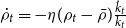 $\dot \rho _t= -\eta (\rho _t-\bar \rho ) \frac {\dot k_t}{k_t}$
.
Given the initial capital and RTP levels.
 $k_0\gt 0$
and
 $\rho _0\gt 0$
, respectively, the social planner’s maximization problem can be summarized as follows:
 \begin{eqnarray} \max _{c_t,\tau _t}\quad W = \int _0^\infty \frac {c_t^{1-\sigma }}{1-\sigma } {e^{-\int _0^t\rho _s ds}} dt \end{eqnarray}
 \begin{eqnarray}\quad\quad\,\quad s.t.\quad \dot k_t =(1-\tau _t)\left (\frac {\tau _t}{\lambda }\right )^{\frac {\chi \omega }{1-\chi \omega }}{\frac {A}{\xi }} k_t -c_t \end{eqnarray}
 \begin{eqnarray}\!\!\!\!\!\quad\, \dot \rho _t= -\eta (\rho _t-\bar \rho ) \frac {\dot k_t}{k_t}, \end{eqnarray}
where
 $\lambda =\frac {\phi \xi }{\theta }\gt 0$
quantifies the relative environmental inefficiency of production with respect to abatement. Note that our specification of emissions and abatement implies that pollution turns out to be equal to
 $p_t= (\frac {\lambda }{\tau _t})^{\frac {\omega }{1-\chi \omega }}$
, which intuitively increases with the degree of relative environmental inefficiency and decreases with the tax rate. The above problem clearly shows that the tax rate yields non-monotonic effects on disposable income and thus on capital accumulation: on the one hand, a higher tax rate diverts resources away from capital accumulation, while, on the other hand, a higher tax rate allows to finance more abatement which by reducing the environmental damage makes more income available for capital accumulation. The social planner needs to balance these two competing effects by determining the optimal size of the income tax rate.
4. BGP equilibrium
Solving the optimization problem above allows us to characterize the optimal tax rate
 $\tau _t^*$
and the BGP equilibrium, along which output, consumption and capital grow at the same common rate
 $\gamma =\gamma _y=\gamma _c=\gamma _k$
while the tax rate is constant. There results are summarized in the next two propositions.
Proposition 1.
Provided that
 $\chi \lt \frac {1}{\omega }$
, the optimal tax rate is constant and given by the following expression:
 \begin{equation} \tau _t=\tau ^*=\omega \chi \in [0,1]. \end{equation}
Proposition1 shows that whenever the elasticity of the environmental damage is not too large (i,e.,
 $\chi \lt \frac {1}{\omega }$
) then the (unique and constant) optimal tax rate increases with both the elasticity of pollution and the elasticity of the environmental damage. Specifically,
 $\omega$
characterizes the percentage change in environmental pollution that can result from a 1% change in emissions from productive activities which escape the benefits from abatement (or for which there is no abatement spending) while
 $\chi$
denotes the percentage change in potential damage to the environment that can be caused by a 1% change in environmental pollution. Intuitively, these two parameters drive the effectiveness of abatement in lowering pollution and thus in making more resources available for capital accumulation, determining the desirability of income taxation. The other economic and environmental parameters instead are irrelevant for the optimal tax rate. Note that, since the optimal tax rate is constant, also pollution turns out to be constant and equal to:
 $p_t=p^*= (\frac {\lambda }{\tau ^*})^{\frac {\omega }{1-\chi \omega }}$
.Footnote
6
Proposition 2.
Define
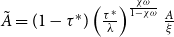 $\tilde A= (1-\tau ^*)\left (\frac {\tau ^*}{\lambda }\right )^{\frac {\chi \omega }{1-\chi \omega }}\frac {A}{\xi }$
and
 $\Theta =\frac {\eta \tilde A}{1-\sigma }$
. Then, there exists a stagnation regime in which the growth rate and the RTP are, respectively, given by
 \begin{eqnarray} \gamma _s=0 \quad \quad \quad \quad \mbox{and} \quad \quad \quad \quad \rho _s^*=\frac {\tilde A + \Theta +\sqrt {(\tilde A+\Theta )^2-4\Theta \bar \rho }}{2}. \end{eqnarray}
Whenever
 $\bar \rho \lt \tilde A \lt \frac {\bar \rho }{1-\sigma }$
, there exists also a growth regime in which the growth rate and the RTP are, respectively, given by
 \begin{eqnarray} \gamma _g=\frac {\tilde A-\bar \rho }{\sigma }\gt 0 \quad \quad \quad \quad \mbox{and} \quad \quad \quad \quad \rho _g^*=\bar \rho. \end{eqnarray}
Proposition2 states that the optimal tax rate determines which development regime will prevail over the long run by driving the effective productivity
 $\tilde A$
. If the condition
 $\bar \rho \lt \tilde A \lt \frac {\bar \rho }{1-\sigma }$
is not verified, then the economy will be trapped in a stagnation regime in which the growth rate is zero (
 $\gamma _s=0$
) such that economic activities remain at subsistence level and the RTP is constant at some level (
 $\rho _s^*$
) which depends on the optimal tax rate. If the condition is verified instead, then the economy will follow a growth regime in which the growth rate is strictly positive (
 $\gamma _g$
) and related to the optimal tax rate while the RTP is constant at a level (
 $\rho _s^*=\bar \rho$
) unrelated to the optimal tax rate. In this latter case, given the AK setting, the optimal tax turns out to be both the growth and welfare maximizing rate, perfectly balancing the beneficial and detrimental effects that income taxation generates on capital accumulation.
Along the growth regime, the growth rate crucially depends on the effective productivity which in turn is driven by the determinants of the optimal tax rate. In particular, it decreases with the relative environmental inefficiency of production with respect to abatement, it increases (decreases) with the elasticity of pollution if
 $\eta \gt \omega$
(if
 $\eta \lt \omega$
), while it is ambiguously related to the damage elasticity parameter. The last result deserves some explanation. On the one hand, an increase in the damage elasticity reduces output via damages, which in turn favors an increase in the tax rate to finance abatement, generating a negative effect on disposable income deterring capital accumulation and growth. On the other hand, a higher tax rate increases abatement reducing pollution and thus increasing the effective productivity, which in turns spurs capital accumulation and growth. The former effect dominates the latter when
 $\chi$
is small, suggesting that growth decreases (increases) for smaller (larger) values of the environmental damage elasticity.
Apart from driving the growth rate along the growth regime, the optimal tax rate plays also a crucial role in determining whether the condition
 $\bar \rho \gt (1-\sigma ) \tilde A$
is met, ultimately controlling which development regime will prevail. Indeed, since the effective productivity depends on the optimal tax rate, whether the growth condition
 $\bar \rho \gt (1-\sigma ) \tilde A$
is verified critically depends also on the elasticities of pollution and environmental damage determining
 $\tau ^*$
. While the effects of
 $\omega$
are intuitive, for the same argument earlier presented the growth regime is compatible only for values of the damage elasticity not too large or too small.
Such results clearly suggest that according to the size of the optimal tax rate a country may end up in a stagnation or growth regime, with diametrically opposite consequences for the standards of living of its population. It may be interesting thus to understand whether differences in the tax rate may explain the differences in development patterns between industrialized and developing countries. In order to shed some light on this, we present a simple parametrization of our model setting most parameters according to values traditionally employed in macroeconomics analysis, with the exception of those that can be calibrated from empirical studies in environmental economics (namely, the pollution elasticity). The steady state RTP in the case of long run growth and the total factor productivity are set as
 $\bar \rho = 0.0267$
and
 $A = 0.0667$
(Strulik, Reference Strulik2012), the elasticity of pollution with respect to unabated emissions as
 $\omega =0.77$
(Liddle, Reference Liddle2015), the inverse of the intertemporal elasticity of substitution as
 $\sigma =0.5$
(Barro, Reference Barro2009), the damage parameter is normalized to one without loss of generality that is
 $\xi =1$
, while the elasticity of the damage function is varied within the interval
 $[0, \frac {1}{\omega }]$
to understand how this parameter affects our results. Indeed, as extensively discussed in literature, the economic consequences of climate change are likely to be highly heterogeneous across countries (Dennig et al., Reference Dennig, Budolfson, Fleurbaey, Siebert and Socolow2015; IPCC, 2022), thus we capture this possibility by considering different values of the elasticity of the damage function. The relative environmental inefficiency of production with respect to abatement is assumed to take one of three values lower than unity to represent the fact that one unit of output allocated to abatement reduces pollution relatively less than the emissions it generates, and specifically we consider
 $\lambda =\{0.3,0.4,0.5\}$
.
Effects of the damage elasticity parameter
 $\chi$
on the optimal tax rate (left) and on the growth rate (right) for low (dotted), mid (dashed) and high (solid) values of
 $\lambda$
.

Figure 1 shows how the optimal tax rate
 $\tau ^*$
(left panel) and the growth rate
 $\gamma$
(right panel) change with the elasticity parameter, for
 $\lambda =0.3$
(dotted curve),
 $\lambda =0.4$
(dashed curve) and
 $\lambda =0.5$
(solid curve). Clearly, a higher damage elasticity increases the tax rate as it raises the environmental damage generated by pollution providing the planner with stronger incentives to abate. However, a higher damage elasticity generates non-monotonic effects on the growth rate and it determines whether the condition
 $\bar \rho \gt (1-\sigma )\tilde A$
holds true or not, and thus whether the economy develops along a growth or a stagnation regime (see Proposition2).
We can observe that for low and high elasticity values the economy follows a stagnation regime along which the growth rate is zero, while for intermediate values it follows a growth regime along which the growth rate and elasticity relation is U-shaped. Outside the parameter region in which the economy develops along a growth regime, the tax rate turns out to be too low or too high to start off an economic take off, consigning the economy to permanent stagnation. Along the growth regime, the growth rate is U-shaped related to the elasticity of the environmental damage, as at lower levels the growth-detrimental effect of income taxation through a subtraction of resource availability dominates while at higher levels its growth-enhancing effect through an improvement in production capabilities does. Moreover, we can observe that the more inefficient the abatement technology (i.e., the higher
 $\lambda$
) the higher are pollution and damages, which slow down capital accumulation and growth. Intuitively, this is related to the fact that a higher degree of environmental inefficiency increases pollution, generating larger damages and thus slowing down capital accumulation and growth. Also, it is interesting to notice that the more inefficient the capacity to abate, the higher the tax rate required for growth to pick up, explaining why the turning point of the growth rate shifts rightward when
 $\lambda$
increases.
In order to get a better understanding of the implications of the heterogeneous consequences of climate change across countries, we now specify our baseline parametrization to distinguish between developed and developing countries.Footnote
7
Indeed, our previous analysis is based on a world level estimate of the elasticity of pollution, while empirical studies demonstrate the existence of a broad variability. Therefore, by focusing on the
 $\lambda =0.4$
case, we now consider a parametrization based on OECD and non-OECD countries, in which
 $\omega =0.71$
and
 $\omega =0.83$
, respectively (Liddle, Reference Liddle2015). As this parameter captures the amount of pollution that escapes abatement, such a parametrization intuitively suggests that in industrialized countries abatement activities are more effective than in developing countries, that is either their abatement technology is more advanced or their allocation of resource to abatement is higher. This might be related to two sorts of issues: developing countries may find difficult to finance abatement spending because of inadequate tax revenues (due to tax evasion, poor tax administration, etc.), and they may face important challenges to pursue abatement activitiesFootnote
8
(such as significant upfront investment and operational expenses, lack of technical expertise and skilled workforce, lack of the necessary infrastructure for transportation and storage).
We report in Figure 2 the results of our analysis in which OECD and non-OECD countries are represented by the purple and light blue curves, respectively. From a qualitative perspective, all our previous conclusions still apply but we can also observe some important differences between the two groups of countries: (i) independent of the size of the damage elasticity, the optimal tax rate in non-OECD countries is larger than in OECD countries and (ii) the region in which the growth regime applies is smaller in non-OECD than in OECD countries. Intuitively, the larger elasticity of pollution in developing countries requires more effort than in developed economies to address its detrimental consequences on production capabilities, but this per se is a first factor of concern given the lack of resources for environmental protection that typically affects poorer countries. Even if the required resources to finance abatement are found, the effectiveness of environmental protection in promoting economic development is uncertain as this largely depends on the elasticity of the environmental damage: for middle-range values economic growth may turn out positive and even substantially higher than in richer countries, but for larger values economic growth may turn out to be zero while in richer countries it may continue to remain positive. Since the consequences of climate change are predicted to be more severe in developing than in developed countries, this brings a second factor of concern as the latter outcome is more likely to occur: developing countries may get stuck in a stagnation regime while industrialized economies continue to prosper, giving rise to growing income inequalities between richer and poorer countries. These results combined suggest that environmental outcomes may play a crucial role in driving economic development, and cross-country heterogeneity may be a source of long-run divergence.Footnote 9
Effects of the damage elasticity parameter
 $\chi$
on the optimal tax rate (left) and on the growth rate (right) in OECD (purple) and non-OECD (light blue) countries.

These results clearly show that the prospects of economic development at the national level may largely depend on the intensity of the environmental damages, which, by driving the optimal tax rate, ultimately determines whether an economy will experience stagnation or growth. Therefore, understanding the heterogeneous effects of climate change on national economic productivity is essential for international organizations to effectively plan and coordinate climate mitigation efforts.
5. Productive public spending
We now extend our baseline framework to account for the role of productive public spending and how the allocation of the tax revenue between abatement and spending affects our conclusions. By maintaining a balanced budget at any time, we now assume that the government uses the collected tax revenue partly to finance pollution abatement and partly to finance productive government spending. Specifically, a share
 $0\lt \varphi \lt 1$
is exogenously allocated to abatement,
 $a_t=\varphi \tau _t y_t$
and the remaining share
 $1-\varphi$
to spending
 $g_t = (1-\varphi ) \tau _t y_t$
. Government spending enters the production function as follows:
 $q_t=A_tk^\alpha g_t^{1-\alpha }$
, which implies that
 $g_t= [(1-\varphi )A]^{\frac {1}{\alpha }}\tau _t^{\frac {1}{\alpha }} k_t$
and thus
 $q_t=A^{\frac {1}{\alpha }} (1-\varphi )^{\frac {1-\alpha }{\alpha }}\tau _t^{\frac {1-\alpha }{\alpha }} k_t$
. Therefore, the social planner’s maximization problem can be written as follows:
 \begin{align} \max _{c_t,\tau _t}\quad W &= \int _0^\infty \frac {c_t^{1-\sigma }}{1-\sigma } {e^{-\int _0^t\rho _s ds}} dt \end{align}
 \begin{align} s.t.\quad \dot k_t &=(1-\tau _t) \left (\frac {\tau _t}{\lambda ^g}\right )^{\frac {\chi \omega }{1-\chi \omega }}\frac {A^{\frac {1}{\alpha }}}{\xi } (1-\varphi )^{\frac {1-\alpha }{\alpha }}\tau _t^{\frac {1-\alpha }{\alpha }} k_t -c_t \end{align}
 \begin{align} \dot \rho _t &= -\eta (\rho _t-\bar \rho ) \frac {\dot k_t}{k_t}, \end{align}
where
 $\lambda ^g=\frac {\lambda }{\varphi }\gt 0$
. As in our baseline model, pollution depends on time only through the tax rate and is equal to:
 $p_t= (\frac {\lambda ^g}{\tau _t})^{\frac {\omega }{1-\chi \omega }}$
. Note that whenever
 $\varphi =1$
and
 $\alpha =1$
the problem above reduces to our baseline formulation.
It is straightforward to observe that the introduction of public spending does not change the main structure of the model and thus most of our previous conclusions will still apply also in such an extended framework. In particular, it is possible to show that the optimal tax rate is still constant (see Proposition1) and that there may still exist a stagnation and a growth regime according to the value of the effective productivity (see Proposition2). Since the optimal tax rate is constant, also pollution turns out to be constant, exactly as before. The next proposition summarizes our conclusions in this context.
Proposition 3.
Provided that
 $\chi \lt \frac {1}{\omega }$
, the optimal tax rate is given by:
 \begin{equation} \tau _t=\tau ^*= \frac {(1-\alpha )(1-\chi \omega )+\alpha \chi \omega }{1-\chi \omega (1-\alpha )}\in [0,1]. \end{equation}
By defining
 $\widetilde A = (1-\tau ^*) \left (\frac {\tau ^*}{\lambda ^g}\right )^{\frac {\chi \omega }{1-\chi \omega }}\frac {A^{\frac {1}{\alpha }}}{\xi } (1-\varphi )^{\frac {1-\alpha }{\alpha }}(\tau ^*)^{\frac {1-\alpha }{\alpha }}$
and
 $\Theta =\frac {\eta \tilde A}{1-\sigma }$
, a stagnation regime where the growth rate and the RTP are given as in (5) always exists, while a growth regime where the growth rate and the RTP are given as in (6) exists only if
 $\bar \rho \lt \tilde A \lt \frac {\bar \rho }{1-\sigma }$
.
Proposition3 confirms that from a qualitative point of view the results earlier presented still apply, even if from a quantitative point of view there are some notable differences in the size of the optimal tax rate and the effective productivity. In particular, it is straightforward to show that in the presence of productive public spending the optimal tax rate is larger than in its absence: analytically, the difference between the optimal tax rates given by (10) and (4) is
 $(1-\alpha )(1-\omega \chi )^2 \gt 0$
, which is always positive as long as
 $\chi \lt \frac {1}{\omega }$
. Intuitively, this is due to the fact that the possibility to use taxes to finance not only abatement but also productive activities strengthens the planner’s motive to increase the tax rate.Footnote
10
How this in turn affects the effective productivity depends on the capital share: for realistic values of the capital share (i.e.,
 $\alpha \leq 0.5$
), the higher optimal tax rate reduces the effective productivity, meaning that it is more difficult for the growth regime to kick in. Therefore, everything else the same, a higher total factor productivity is required to allow for sustained growth.
In order to better understand the implications of productive public spending on the long run development patterns, it may be convenient to return to our (world-level) baseline calibration. By maintaining the parameter values as before with the exception of the total factor productivity which is set as
 $A=1$
(the previous value of
 $A = 0.0667$
is too low for sustained growth to occur) and considering the
 $\lambda =0.4$
case, we can set the capital share as
 $\alpha =0.4$
(Feenstra et al., Reference Feenstra, Inklaar and Timmer2015) in order to understand how different values of the share of taxes allocated to abatement affects our conclusions. Specifically, we consider the following values
 $\varphi =\{0.5,0.55,0.6\}$
.
Effects of the damage elasticity parameter
 $\chi$
on the optimal tax rate (left) and on the growth rate (right) for low (dotted), mid (dashed) and high (solid) values of
 $\varphi$
.

Figure 3 shows how the optimal tax rate
 $\tau ^*$
(left panel) and the growth rate
 $\gamma$
(right panel) change with the elasticity parameter
 $\chi$
, for
 $\varphi =0.5$
(dotted curve),
 $\varphi =0.55$
(dashed curve) and
 $\varphi =0.6$
(solid curve). Different from what we have discussed in the absence of productive public spending (see Figure 1), we can observe that the range of
 $\tau ^*$
is quite narrow suggesting that the optimal tax rate is less affected by the elasticity of the damage function; moreover, the value of
 $\tau ^*$
is substantially higher than in the absence of public spending. Making a comparison of the growth rates is difficult as the size of the total factor productivity is now different from our baseline framework. Nevertheless, we can conclude that the growth rate is still non-monotonically related to
 $\chi$
; thus most of our previous comments still apply with the only difference related to the fact that the detrimental effect of income taxation on capital accumulation is balanced by two different beneficial effects on production, one through effective productivity as in our baseline setup and the other through productive public spending. Note also the dual role of
 $\varphi$
: a higher share of taxes allocated to abatement reduces growth but increases the size of the growth regime region, making thus more likely for growth to occur.Footnote
11
Extending the analysis to account for productive public expenditure, we can conclude that the intensity of the environmental damages still plays a fundamental role in determining the prospects of economic development at national level, but also governments’ role in mitigating the heterogeneous effects of climate change across countries is important. Indeed, an effective productive use of tax revenues may help economies escaping the stagnation regime, completely changing their long run development patterns.
6. Clean and dirty capital
We now extend our analysis to understand how the presence of two forms of capital (dirty and clean capital) affects our conclusions. Since the presence of productive government spending does not qualitatively modify our results, we return to our baseline model for the sake of simplicity, and we now assume that there exist dirty
 $k_t$
and clean
 $h_t$
capital goods. Emissions are proportional to dirty capital, and clean capital does not contribute to emissions at all:
 $e_t=\phi k_t$
. Output is produced through a Cobb-Douglas production technology as follows:
 $q_t=Ak_t^\alpha h_t^{1-\alpha }$
, where
 $0\lt \alpha \lt 1$
is the dirty capital share of output. Income, which as in our baseline framework equals production net of environmental damage
 $y_t = \frac {q_t}{d_t}$
, can be allocated to consumption, investment in dirty capital accumulation
 $i_{k,t} = \dot k_t$
, investment in clean capital accumulation
 $i_{h,t} = \dot h_t$
, or government spending as follows:
 $y_t = c_t + i_{k,t} +i_{h,t} + g_t$
. Due to our formulation of abatement, pollution is now expressed as follows:
 $p_t= (\frac {\lambda }{\tau _t})^{\frac {\omega }{1-\chi \omega }} [A(\frac {h_t}{k_t})^{1-\alpha }]^{-\frac {\omega }{1-\chi \omega }}$
which, different from our baseline specification, does not depend only on the tax rate but also on the ratio between clean and dirty capital
 $\frac {h_t}{k_t}$
. It follows that income turns out to be given by the following expression:
 $y_t=\left (\frac {\tau _t}{\lambda }\right )^{\frac {\chi \omega }{1-\chi \omega }}\frac {A^{\frac {1}{1-\chi \omega }}}{\xi } k_t^{\widetilde \alpha } h_t^{1-\widetilde \alpha }$
where
 $\widetilde \alpha =\frac {\alpha -\chi \omega }{1-\chi \omega }\in (0,1)$
provided that
 $\alpha \gt \chi \omega$
. Straightforward algebra (see Barro and Sala-i-Martin, Reference Barro and Sala-i-Martin2004, section 5.1) allows us to show that at equilibrium the ratio between clean and dirty capital turns out to be constant and equal to:
 $\frac {h_t}{k_t}=\frac {1-\widetilde \alpha }{\widetilde \alpha }$
, which implies that income is proportional to dirty capital:
 $y_t=\left (\frac {\tau _t}{\lambda }\right )^{\frac {\chi \omega }{1-\chi \omega }}\frac {A^{\frac {1}{1-\chi \omega }}}{\xi } (\frac {1-\widetilde \alpha }{\widetilde \alpha })^{1-\widetilde \alpha } k_t$
. At equilibrium the social planner’s problem can thus be written as:
 \begin{align} \max _{c_t,\tau _t}\quad W &= \int _0^\infty \frac {c_t^{1-\sigma }}{1-\sigma } {e^{-\int _0^t\rho _s ds}} dt \end{align}
 \begin{align} s.t.\quad \dot k_t &=(1-\tau _t)\left (\frac {\tau _t}{\lambda }\right )^{\frac {\chi \omega }{1-\chi \omega }}\frac {A^{\frac {1}{1-\chi \omega }}}{\xi } \widetilde \alpha ^{\widetilde \alpha } (1-\widetilde \alpha )^{1-\widetilde \alpha }k_t -\widetilde \alpha c_t \end{align}
 \begin{align} \dot \rho _t &= -\eta (\rho _t-\bar \rho ) \frac {\dot k_t}{k_t}, \end{align}
Also in this case, we can observe that the introduction of an additional form of capital does not change the main structure of the model, and thus most of our previous conclusions will still apply. In particular, it is possible to show that the optimal tax rate is still constant and given by (4) (exactly as in Proposition1) and that there may still exist a stagnation and a growth regime according to the value of the effective productivity (see Proposition2). Since the optimal tax rate and the clean and dirty capital ratio are constant, also pollution turns out to be constant along the BGP equilibrium. The next proposition summarizes our conclusions.
Proposition 4.
Provided that
 $\chi \lt \frac {\alpha }{\omega }$
, and defining
 $\widetilde A = (1-\tau ^*)\left (\frac {\tau ^*}{\lambda }\right )^{\frac {\chi \omega }{1-\chi \omega }}\frac {A^{\frac {1}{1-\chi \omega }}}{\xi } \widetilde \alpha ^{\widetilde \alpha } (1-\widetilde \alpha )^{1-\widetilde \alpha }$
and
 $\Theta =\frac {\eta \tilde A}{1-\sigma }$
with
 $\tau ^*$
being given by (
4
), a stagnation regime where the growth rate and the RTP are given as in (5) always exists, while a growth regime where the growth rate and the RTP are given as in (6) exists only if
 $\bar \rho \lt \tilde A \lt \frac {\bar \rho }{1-\sigma }$
.
Proposition4 confirms from a qualitative point of view all the results we have presented in our baseline analysis. A relevant difference is related to the size of the damage elasticity which now is restricted to take smaller values than in our baseline setup. Another and more important difference concerns the effective productivity, which is affected by the dirty capital share of output through its effects on
 $\widetilde \alpha$
. This turns out to be larger or smaller than in our baseline framework according to the specific parametrization, and in particular the total factor productivity, the elasticity of pollution and the elasticity of the environmental damages play a critical role in this context and therefore in determining whether the growth or the stagnation regime will prevail.
Different from what we have discussed before, however, the fact that pollution is related to the ratio of the stocks of dirty and clean capital introduces a wedge between the growth rate in the centralized and decentralized economies. Indeed, in a competitive equilibrium the effective productivity would read as
 $\tilde A' = (1-\tau ^*)\left (\frac {\tau ^*}{\lambda }\right )^{\frac {\chi \omega }{1-\chi \omega }}\frac {A^{\frac {1}{1-\chi \omega }}}{\xi } \alpha ^{\widetilde \alpha } (1-\alpha )^{1-\widetilde \alpha }$
and the growth rate as
 $\gamma _g'=\frac {\tilde A'-\bar \rho }{\sigma }\gt 0$
. Since
 $\alpha \gt \widetilde \alpha$
, it follows that
 $\tilde A' \lt \tilde A$
which implies that the growth rate under a centralized economy exceeds the growth rate in a decentralized context (i.e.,
 $\gamma _g\gt \gamma _g '$
). This is due to the fact that, by internalizing the environmental externality, the social planner chooses to opt for a higher clean to dirty capital ratio than in a decentralized setting (under decentralization
 $(\frac {h_t}{k_t})'=\frac {1-\alpha }{\alpha }$
holds true), and this results in lower pollution, lower damages and thus higher production capability. Note that even if the level of emissions abatement is the same since the tax rate coincides under centralization and decentralization, the possibility to divert income from financing dirty to clean capital accumulation allows the social planner to achieve faster long run growth. In particular, the size of the inefficiency induced by agents’ failure to internalize the externality is equal to
 $\varpi = \widetilde \alpha ^{\widetilde \alpha } (1-\widetilde \alpha )^{1-\widetilde \alpha } - \alpha ^{\widetilde \alpha } (1-\alpha )^{1-\widetilde \alpha }$
, which intuitively increases with the pollution and damage elasticity parameters. The introduction of non-distortionary lump sum subsidies (taxes) of size
 $\varpi$
to favor (deter) the accumulation of clean (dirty) capital would allow to restore the first best by equating the equilibrium clean to dirty capital ratio in the decentralized economy to its socially optimal value.
Since, from a qualitative point of view, our results are robust even to the introduction of two alternative forms of capital, we can reiterate our conclusions about the importance of the magnitude of environmental damages in determining the prospects of economic development at a national level, along with the essential role that policymakers may play in mitigating the heterogeneous effects of climate change across countries. Indeed, an effective use of transfers may help the decentralized economy to internalize externalities to replicate the social optimum and promote faster long-run growth.
7. Conclusions
In this paper we have considered an endogenous growth model where production activities generate emissions and pollute the environment, and abatement spending is undertaken to reverse the pollution damages. A utilitarian government sets the income tax rate optimally to raise tax revenues, which are the only source for financing abatement. The RTP is not constant but varies negatively with the stock of capital, implying that environmental outcomes and thus income taxation indirectly affect the evolution of the RTP through their effects on production capabilities. We show that, despite the environment not affecting either utility or impatience directly, environmental parameters determine the optimal tax rate and thereby ascertain whether the economy will either be stuck in a stagnation regime or prosper in a growth regime, and the existence of those two regimes is ensured by the endogeneity of the RTP. In the growth regime, a higher elasticity of environmental damages leads to non-monotonic effects on economic growth, via their implications on the optimal tax rate and thus on both production capabilities and abatement. These findings suggest that cross-country heterogeneity in environmental damages may explain the different developmental patterns followed by industrialized and developing economies, through their implications for the optimal tax rate and thus on the prevalence of a stagnation or growth regime. We show that our conclusions are robust even to the introduction of productive public expenditure, and two alternative forms of capital (clean and dirty capital), confirming the importance of environmental damages in determining the long-run prospects of economic development along with the essential role of public policy in effectively guiding the economy towards a more prosperous regime.
It is important to stress that our analysis is based on some key modeling assumptions which may limit the generalizability of our conclusions. While most of our assumptions are rather standard and consistent with extant literature, the specification of pollution and of a closed economy setting deserve some comments. In fact, we have assumed that pollution is a flow (and not a stock) variable; thus we cannot account for pollutants with long-lasting effects such as CO2, and since CO2 is the major driver of climate change, our discussion about the role of climate change in determining heterogeneity between countries represents only a simplistic description of a much more complicated reality. Moreover, the absence of international resource flows between countries implies that we cannot account for the transboundary nature of pollution which gives rise to free riding and strategic interactions between countries, suggesting that our conclusions may fail to capture important issues underlying the problems associated with international cooperation. Despite such limitations, we believe that our framework represents a useful starting point to explore how environmental outcomes, capital accumulation and impatience are related to public policy,Footnote 12 and what such a relation may imply for the future prospects of economic development both in industrialized and developing countries.
In order to present our arguments in the most intuitive way we have developed a very stylized model abstracting from several important issues. In particular, we have not considered the role of human capital, which by improving the efficiency of abatement may allow the tax rate to decrease to reduce the production externality, favoring a faster capital accumulation and reduction in impatience, yielding more favorable prospects for long-run economic development. Moreover, one can think of environmental policy not being restricted to abatement only, in which case policymakers may favor economic prosperity also by promoting green innovations or the adoption of green behaviors, affecting the environment, capital accumulation and impatience. Extending the analysis along these directions is left for future research.
Acknowledgements
We wish to thank two anonymous reviewers for their constructive comments and valuable suggestions on earlier drafts. We are grateful to participants at the 18th Annual Conference on Economic Growth and Development at Indian Statistical Institute, New Delhi, in December 2023, at the Scottish Economic Society Annual Conference at University of Glasgow in April 2024, and at a departmental seminar at University of Graz, Austria, in April 2024, for insightful discussions. The usual disclaimer applies.
Appendix A. Equilibrium and Transitional Dynamics
By defining
 $\phi \equiv \int _0^t \rho _s ds$
and
 $\varphi _{it}$
with
 $i=\{k, \rho \}$
the costate variables for capital and RTP, respectively, the Hamiltonian function associated with the problem (11), (12) and (13) reads as follows:
 \begin{eqnarray*} \mathcal{H}(c_t, \tau _t, k_t, \rho _t)=\frac {c_t^{1-\sigma }}{1-\sigma } e^{-\phi } + \varphi _{kt}\left [(1-\tau _t)\left (\frac {\tau _t}{\lambda }\right )^{\frac {\chi \omega }{1-\chi \omega }}A k_t -c_t\right ] - \varphi _{\rho t} \rho _t \end{eqnarray*}
First order necessary and sufficient (it is possible to prove that the Hamiltonian is concave) conditions turn out to be:
 \begin{eqnarray*} & &c_t^{-\sigma }e^{-\phi }= \varphi _{kt}\\ & &\varphi _{kt} A k_t \left [\tau _t - \omega \chi \right ] = 0\\ & &-\dot {\varphi _{kt}}=\varphi _{kt} (1-\tau _t)\left (\frac {\tau _t}{\lambda }\right )^{\frac {\chi \omega }{1-\chi \omega }}A - \varphi _{\rho t} \rho _t'\\ & &-\dot {\varphi _{\rho t}}=-\frac {c_t^{1-\sigma }}{1-\sigma } e^{-\phi } \end{eqnarray*}
From the second equation above, straightforward algebra implies that
 $\tau _t^* = \tau ^* =\omega \chi$
(see Proposition1). The first equation can be rewritten as
 $c_t^{-\sigma }= \widetilde \varphi _{kt}$
where
 $\widetilde \varphi _{kt}\equiv \varphi _{kt} e^{\phi }$
, and taking logs of the former expression yields
 $-\sigma \ln c_t=\ln \widetilde \varphi _{kt}$
which after differentiating with respect to time results in
 $\frac {\dot {\widetilde \varphi _{kt}}}{\widetilde \varphi _{kt}}=-\sigma \frac {\dot c_t}{c_t}$
. After some manipulations, the transversality condition
 $\lim _{t\to \infty }\mathcal{H}=0$
leads to
 $\frac {\widetilde \varphi _{\rho t}}{\widetilde \varphi _{kt}}\rho = \frac { c_t}{1-\sigma }+\tilde A k_t -c_t$
, where
 $\tilde A= (1-\tau ^*)\left (\frac {\tau ^*}{\lambda }\right )^{\frac {\chi \omega }{1-\chi \omega }}\frac {A}{\xi }\gt 0$
and
 $\widetilde \varphi _{\rho t}=\varphi _{\rho t} e^{\phi }$
. Time-differentiating
 $\widetilde \varphi _{k t}$
and substituting into
 $\frac {\dot {\widetilde \varphi _{kt}}}{\widetilde \varphi _{kt}}=-\sigma \frac {\dot c_t}{c_t}$
(see Strulik, Reference Strulik2012), yields
 $\frac {\dot c_t}{c_t}= \frac {1}{\sigma } [\tilde A -\rho _t - \frac {\rho _t'}{\rho _t} \frac { c_t}{1-\sigma } - \frac {\rho _t'}{\rho _t} (\tilde A k_t -c_t)]$
. Next, using
 $\rho _t= \bar \rho + \rho _0 k_t^{-\eta }$
we obtain
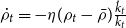 $\dot \rho _t= -\eta (\rho _t-\bar \rho )\frac {\dot k_t}{k_t}$
, and hence
 $\frac {\dot c_t}{c_t}= \frac {1}{\sigma } [\tilde A -\rho _t + \frac {\eta }{1-\sigma } (\frac {\rho _t-\bar \rho }{\rho _t} ) \frac {c_t}{k_t}+\eta (\frac {\rho _t-\bar \rho }{\rho _t} )\frac {\dot k_t}{k_t}]$
. Finally, the dynamics of the consumption to capital ratio
 $\psi _t=\frac {c_t}{k_t}$
and of the RTP can be written as in the following expressions:
 \begin{eqnarray*} \frac {\dot \psi _t}{\psi _t}&=& \frac {1-\sigma }{\sigma } \tilde A +\psi _t - \frac {\rho _t}{\sigma } + \frac {\eta }{\sigma } \left (\frac {\rho _t-\bar \rho }{\rho _t} \right ) \left ( \tilde A +\frac {\sigma }{1-\sigma }\psi _t\right )\\ \dot \rho _t&=& -\eta (\rho _t-\bar \rho )\left (\tilde A - \psi _t \right ) \end{eqnarray*}
By setting the LHS of the previous equations equal to zero, we can obtain the two steady state equilibria given by
 $E_s=(\psi _s^*,\rho _s^*)$
and
 $E_g=(\psi _g^*,\rho _g^*)$
, which are associated with the stagnation and growth regimes, respectively (see Proposition2), and where
 $\psi _s^*= \tilde A$
,
 $\rho _s^*=\frac {\tilde A + \Theta +\sqrt {(\tilde A+\Theta )^2-4\Theta \bar \rho }}{2}$
,
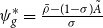 $\psi _g^*=\frac {\bar \rho - (1-\sigma )\tilde A}{\sigma }$
, and
 $\rho _g^*=\bar \rho$
, with
 $\Theta =\frac {\eta \tilde A}{1-\sigma }$
. While equilibrium
 $E_s$
exists and is well defined for all parameter values, equilibrium
 $E_g$
does only whenever
 $\bar \rho \gt (1-\sigma )\tilde A$
. Note that there exists another positive solution of the quadratic equation in
 $\rho _t$
, but this is infeasible since it implies a value of the RTP lower than
 $\bar \rho$
, which instead represents the minimal RTP associated with non-negative capital.
Linearization around the steady states shows that
 $E_s$
is locally unstable while
 $E_g$
is saddle point stable, suggesting that whenever
 $E_g$
exists in the long run the economy converges to the growth regime while when it does not the economy develops from time zero along the stagnation regime.
B. Sensitivity Analysis
We now perform some sensitivity analysis to show the extent to which the results of our calibration depend on the specific parametrization employed. We focus on the main parameters affecting the optimal tax rate and the growth rate in our benchmark model, which are the inverse of the intertemporal elasticity of substitution, the total factor productivity, and the pollution elasticity. We return to our baseline (world-level) parametrization showing how the results may differ from those presented in Figure 1.
Effects of the damage elasticity parameter
 $\chi$
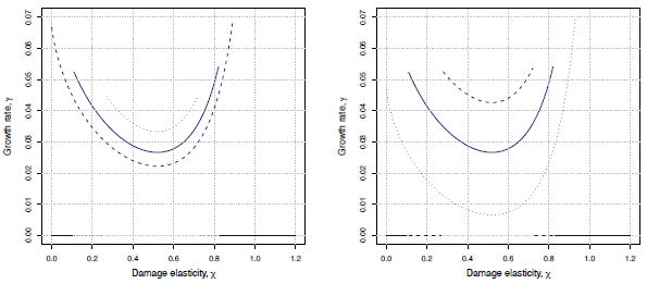
on the growth rate when the intertemporal elasticity of substitution (left) and the total factor productivity (right) change, among high values (dashed), middle values (solid) and low values (dotted).

Since the intertemporal elasticity of substitution and the total factor productivity do not affect the optimal tax rate, irrespective of their value the tax rate is still as in the left panel of Figure 1; thus we shall focus only on how these parameters affect the growth rate. We consider three values for each of these parameters, and specifically
 $\sigma =\{0.4,0.5,0.6\}$
and
 $A=\{0.05,0.0667, 0.08\}$
, where the low and high values are determined around the mid-value employed in our benchmark analysis. Figure B1 reports the results of our analysis in the case of variations in
 $\sigma$
(left panel) or
 $A$
(right panel), distinguishing high (dashed) from middle (solid) and low (dotted) values of the relevant parameter. We can observe that qualitatively the growth pattern is consistent with what we have discussed in the main text. What may be relevant to mention is that the two parameters have completely different effects on the growth rate: the intertemporal elasticity of substitution decreases the growth rate within the region that characterizes the growth regime but expands the size of the growth regime itself, while the total factor productivity increases the growth rate within the growth regime region but reduces the size of the region defining the growth regime. This result straightforwardly follows from the Proposition2 by noting the role of
 $\sigma$
and
 $A$
in determining the (positive) growth rate and the effective productivity.
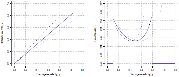
Effects of the damage elasticity parameter
 $\chi$
on the optimal tax rate (left) and on the growth rate (right) for
 $\omega =0.69$
(dashed),
 $\omega =0.81$
(solid) and
 $\omega =0.99$
(dotted).

Less obvious instead is the role of the pollution elasticity, since it affects both the optimal tax rate and the growth rate. As this is the main parameter which drives our analysis, in the following we shall rely on different empirical estimates to understand its role in affecting our conclusions. In our benchmark analysis we have set this parameter according to the world-level estimate of the emissions elasticity with respect to affluence based on the augmented mean group estimator (AMG) as in Liddle (Reference Liddle2015). Liddle (Reference Liddle2015) also estimates the same parameter by relying on the common correlated effects mean group estimator (CMG), and these different set-ups give rise to quite different estimates. For our analysis, since we have already employed the AMG point estimate in Figure 1, we rely on the CMG point estimate and the extremes (minimum and maximum) of the AMG and CMG interval estimates. Specifically, we set
 $\omega =\{0.69,0.81,0.99\}$
and Figure B2 reports the results of our analysis distinguishing the effects of high (dashed) from middle (solid) and low (dotted) values of the parameter on the optimal tax rate (left panel) and the growth rate (right panel). Also in this case qualitatively the results are consistent with those already discussed in the main text. Intuitively, the pollution elasticity increases the optimal tax rate (see Proposition1) but its effects on growth are not obvious. Within the region characterizing the growth regime (which reduces its size with the pollution elasticity), at low values of
 $\omega$
the pollution elasticity decreases the growth rate while at higher values of
 $\omega$
the pollution elasticity increases the growth rate. This is due to the non-monotonic effects of
 $\chi$
on
 $\gamma _g$
and how
 $\omega$
interacts with them, similar to what we have discussed in the text.
Overall, from a qualitative point of view, our sensitivity analysis confirms our main conclusions suggesting that the results of our benchmark analysis apply in a wide range of parameter values consistent with previous studies in macroeconomics and environmental economics.