3.1. Flow characteristics

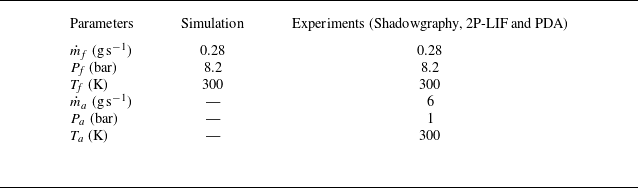
The CORIA Rouen spray burner (CRSB) was employed for both numerical simulations and experimental measurements conceived to capture the atomisation process of n-heptane. The burner configuration is schematically shown in figure 1(a). It consists of a fuel injection system and a plenum. The fuel injector is placed at the centre of the injection system and is surrounded by a co-flowing air stream guided through a convergent annular passage. The downstream end of the annular passage has an outer diameter of 20 mm and an inner diameter of 10 mm. Its upstream end is connected to the plenum, which houses 18 radial vanes set at zero degrees. The radial vanes serve to break up large-scale airflow structures. Additional details on the burner geometry are available from Verdier et al. (Reference Verdier, Santiago, Vandel, Godard, Cabot and Renou2018).

Figure 1.

(a) Schematic of the CRSB, highlighting key dimensions in millimetres. To enable optical access from the atomiser outlet, the injector is positioned 2.02 mm downstream. (b) Juxtaposition of instantaneous images of both numerically simulated and experimentally captured hollow-cone sprays generated by this injection system.

The industrial pressure-swirl atomiser (manufactured by Danfoss, model 030H8306) integrated with the CRSB is rated for a flow rate of 1.35 kg h $^{-1}$ , shaping an 80 $^{\circ }$ hollow-cone spray. The internal geometry of the injector ensures that part of the fuel pressure generates a rotating liquid film along the injector walls, which then leads to the orifice, while the remaining pressure forces the liquid through the orifice as a conical sheet into the co-flowing air. For all experiments, n-heptane was injected under operating conditions of injection pressure $P_{\!f}$ = 8.2 bar and mass flow rate $\dot {m}_{\!f}$ = 0.28 g s $^{-1}$ at room temperature. The air co-flow was $\dot {m}_a$ = 6 g s $^{-1}$ at atmospheric conditions. Please note this co-flow air was not used to atomise the fuel, but it was rather used as an air curtain to minimise surrounding effects on the atomising spray. It was checked experimentally that the influence of co-flow air in the near-injection region was negligible (Sun et al. Reference Sun, Vegad, Li, Renou, Nishad, Demoulin, Wang, Hasse and Sadiki2025) and, as such, it was not prescribed in the simulations. The essential features of the hollow-cone spray structures formed in both numerical simulation and experiments are shown in figure 1(b). For convenience, the common flow conditions and other relevant information are summarised in table 1.

Table 1.

Flow conditions of the hollow-cone spray for simulation and experiments.

Instantaneous images of microscopic shadowgraphy and snapshots of numerical simulations, shown in figure 1(b), capture the primary breakup of the continuous liquid phase into liquid parcels that begin to evolve into ligaments or droplets. Since the present study focuses on the early stage of the spray, where the liquid phase is not fully composed of spherical liquid parcels, the dilution zone, where all liquid parcels disintegrate into fine droplets, lies further downstream and is not included in the images. However, it is worth noting that direct measurements of droplet size up to the dilution zone were performed using phase Doppler anemometry (PDA). These measurements were carried out at different radial locations, from the spray central axis up to the edge of the spray cone, for each axial position in the range of $Z$ = 1–10 mm downstream of the injector outlet. The radial and axial measurement steps were 0.5 and 1 mm, respectively. Data acquisition was limited to 30 s or 120 000 droplets to ensure convergent statistics. The present study aims to compare the predicted spray characteristics obtained from the curvature analysis with PDA measurements. Details on the PDA measurements were reported by Vegad et al. (Reference Vegad, Idlahcen, Huang, Cabot, Renou, Duret, Reveillon and Demoulin2024). For analyses of reacting flows in this burner configuration, interested readers are referred to Verdier et al. (Reference Verdier, Santiago, Vandel, Godard, Cabot and Renou2018) and Mulla & Renou (Reference Mulla and Renou2019).

3.2. Numerical simulation

A volume of fluid (VOF) based LES approach is used to model the atomisation process of a simplex swirl atomiser. The numerical simulation can be considered a DNS-like approach for the liquid phase and the surrounding gas close to the liquid: in these regions, the cell size is small enough to avoid modelling turbulence. Far from the liquid phase, the gas is treated with a LES approach to reduce the computational cost, since modelling every droplet in a full DNS of a real injector would be currently prohibitive. For purely academic test cases, a full DNS could be performed, but for this realistic injector configuration, the hybrid approach provides a practical compromise. The methodology comprises the computation of both internal and external flows. The numerical work was thus performed in two stages: the first simulation addressed the internal flow domain, while the second simulation focused exclusively on a single sector of the 360 $^\circ$ external domain, computed at higher resolution. The data collected at the injector outlet from the first simulation were mapped as a boundary condition for the second simulation. For the internal flow, the dimensions of the internal geometry of the atomiser were obtained with the help of optical microscope visualisation, scanning electron microscopy (SEM) and computed tomography scan (CT-Scan). A detailed characterisation of the internal geometry of the atomiser and its numerical simulation has been reported by Ferrando et al. (Reference Ferrando, Carreres, Belmar-Gil, Cervelló-Sanz, Duret, Reveillon, Salvador and Demoulin2023).

The external flow was simulated by mapping the velocity vector $\boldsymbol{u}(t)$ and the liquid volume fraction $\alpha (t)$ from the internal simulation through a time-varying Dirichlet boundary condition. Figure 2(a) shows contours of the liquid volume fraction at the midplane for both the internal and external domains. Note that the left part of the panel presents the mean field, while the right part displays an instantaneous snapshot. The liquid flow inside the injector was displaced from the central axis throughout the simulation, indicating the presence of an air core, as seen in the mean contours. The instantaneous contours clearly reveal the fluctuations arising within the internal field, which are responsible for the spatiotemporal variations in sheet thickness. A red line in the contour marks the injector outlet, from which $\boldsymbol{u}(t)$ and $\alpha (t)$ were mapped to the external simulation.

Figure 2.

(a) Contours of liquid volume fraction at the midplane for both internal and external domains. The left part displays the averaged contour over a duration of 0.1 ms, while the right part shows the instantaneous fluctuations within both domains. The red line corresponds to the injector outlet from where $\boldsymbol{u}(t)$ and $\alpha (t)$ are extracted and used for the external domain simulation. (b) A 45 $^\circ$ sector of the external geometry domain, showcasing various boundary conditions. The inlet condition is time-dependent and mapped from the internal domain simulation, as indicated by the arrow. No-slip conditions are imposed at the wall, periodic conditions at the side patches and atmospheric pressure at the outlet. (c) A central cross-sectional view of the external domain numerical grid, where the black area features a hollow-cone refinement zone (axial coordinate up to $Z$ = 1.3 mm) designed to accurately capture atomisation processes and liquid–gas interfaces.

Figure 2(b) illustrates the 45 $^\circ$ sector of the external simulation domain, with a height and radius of 4 mm. The inlet surface of the domain has an arc radius equal to the orifice radius, shown in red. The boundary condition at the inlet is defined by $\boldsymbol{u}$ and $\alpha$ as time-varying fixed values (Dirichlet), with $\boldsymbol{\nabla \!}p=0$ (Neumann). Periodic boundary conditions are prescribed at both side patches, and a no-slip boundary condition is imposed at the wall. At the outlet, $\boldsymbol{\nabla \!}u=\boldsymbol{\nabla \!}\alpha =0$ (Neumann), while pressure is prescribed as a total pressure condition (Dirichlet).

Figure 2(c) also presents the computational grid representing the front face (perpendicular to the patches) of the sector domain. A Cartesian isotropic meshing approach is employed, as detailed by Ferrando et al. (Reference Ferrando, Carreres, Belmar-Gil, Cervelló-Sanz, Duret, Reveillon, Salvador and Demoulin2023). As in the internal simulation, second-order schemes are used in both time and space. To better capture the liquid–gas interface, a hollow-cone refinement zone (up to 1.3 mm axial coordinates, without further extension due to limitations in computational resources) is defined following the spray cone angle of approximately 82 $^\circ$ , consistent with the measurements reported by Verdier et al. (Reference Verdier, Santiago, Vandel, Godard, Cabot and Renou2018). This refined mesh zone appears as a dark area in figure 2(c). The cell size within the refinement zone is set to ${\rm d}x$ = 1.2 $\mu$ m (the maximum cell size outside the refinement zone is 50 $\unicode{x03BC}$ m), yielding approximately 8.8 $\times$ 10 $^7$ computational cells in the 45 $^\circ$ sector domain. The rest of the external domain is discretised with progressively coarser refinement levels to reduce the total computational cost. The smallest cell size of 1.2 $\unicode{x03BC}$ m allows resolving droplets down to approximately 4.8 $\mu$ m, while keeping the total number of cells manageable. The coarse mesh region was selected to recover approximately 80 $\,\%$ of the turbulent kinetic energy, as is typical in LES. A constant time step of 8 $\times$ 10 $^{-10}$ s is used, for a total simulated time of 0.1 ms.

The presented simulation is representative of the current state-of-the-art achievements attainable for such a complex configuration. Further details on the numerical set-up, including the determination of the internal flow geometry, the mesh transition strategy ensuring swirl conservation and the numerical schemes employed are reported by Ferrando et al. (Reference Ferrando, Carreres, Belmar-Gil, Cervelló-Sanz, Duret, Reveillon, Salvador and Demoulin2023). That work also provides a detailed comparison with available experimental data, validating the simulation against key macroscopic quantities such as spray angle, liquid film thickness and liquid sheet breakup length, as well as the overall primary breakup mechanism, which agrees with experimental observations (as shown in figure 1). This validated simulation serves as the basis for the surface curvature analysis developed in the present work. The objective here is to assess whether surface curvature analysis applied to such a simulation can effectively describe the atomisation process, by comparison with experiments using, on one hand, a well-established diagnostic technique (PDA) and, on the other, a first attempt to measure the curvature distribution directly by experimental means.

Numerical simulations were carried out using the incompressible VOF-based solver interFoam, available in the OpenFoam 6.0 library. The solver provides the liquid volume fraction $\alpha$ for each computational cell and captures sharp interfaces through the inclusion of sharpening terms in the interface capturing method (ICM). The spray field is described by the mass and momentum conservation equations, given by

(3.1) \begin{align} \frac {\partial \bar {u}_{\!j}}{\partial x_{\!j}} = 0, \end{align}

(3.2) \begin{align} \frac {\partial (\bar {\rho } \bar {u}_i)}{\partial t} + \frac {\partial (\bar {\rho } \bar {u}_{\!j} \bar {u}_i)}{\partial x_{\!j}} = -\frac {\partial \bar {P}}{\partial x_i} + \frac {\partial (\tau _\textit{ij}+\tau _\textit{tij})}{\partial x_{\!j}}+\bar {\rho } g_i + f_{\sigma i}, \end{align}

where, $\bar {u}$ , $\bar {P}$ and $\bar {\rho }$ denote the filtered velocity vector, pressure and density of the computational cell, defined as $\bar {\rho } = \bar {\alpha }\rho _l + (1-\bar {\alpha }) \rho _g$ . The viscous and turbulent stresses, including all sub-grid scale contributions, are represented by $\tau _\textit{ij}$ and $\tau _\textit{tij}$ , respectively. Additionally, $g_i$ is the gravitational acceleration and $f_{\sigma i}$ denotes the surface tension forces, calculated according to a continuum surface force (CSF) approach (Brackbill, Kothe & Zemach Reference Brackbill, Kothe and Zemach1992) as given by

(3.3) \begin{align} f_{\sigma i} = \sigma \kappa \frac {\partial \bar {\alpha }}{\partial x_{\!j}}, \end{align}

where $\sigma$ denotes the surface tension between the liquid and the gas, $\alpha$ represents the liquid volume fraction, and $\kappa$ is the curvature of the surface interface. To determine the interface position, the advection equation for the liquid volume fraction $\alpha$ is solved,

(3.4) \begin{align} \frac {\partial \bar {\alpha }}{\partial t} + \frac {\partial (\bar {\alpha } \bar {u}_{\!j})}{\partial x_{\!j}} = \frac {\partial (U_{j}^r \bar {\alpha })(\bar {\alpha } -1)}{\partial x_{\!j}}, \end{align}

where $U^r = C_{\alpha } |u|(\boldsymbol{\nabla \!}\alpha /|\boldsymbol{\nabla \!}\alpha |)$ denotes the relative velocity used to compress the interface region and maintain a sharp interface (Wardle & Weller Reference Wardle and Weller2013).

The present simulations employ an interface capturing method to track liquid–gas interfaces, together with a single-phase flow LES model to represent the sub-grid stress. The WALE sub-grid model is used to capture flow instabilities in wall boundary layers for liquid–gas flows with low mesh resolution. The liquid–gas interface is captured through a sharpening interface term in the right-hand side of the liquid volume fraction advection equation (3.4). The LES framework and the WALE sub-grid scale model are retained from the internal simulation (see Ferrando et al. Reference Ferrando, Palanti, Demoulin, Duret and Reveillon2021). A 45 $^\circ$ sector of the simulated spray after a 360 $^\circ$ swipe is illustrated in figure 2(b). It should be noted that no instantaneous snapshot is used for the curvature analysis of the simulated spray; the methodology proposed by Palanti et al. (Reference Palanti, Puggelli, Langone, Andreini, Reveillon, Duret and Demoulin2022) is instead applied, as explained in § 4.

3.3. Experimental diagnostics

3.3.1. Test bench

The schematic of the experimental setup developed to produce n-heptane atomisation is shown in figure 3(a). Fuel and air are supplied to the CRSB according to the conditions in table 1, using a Coriolis mass flow controller (Bronkhorst, CORI-FLOW, 0–2 g s $^{-1}$ ) and a thermal mass flow controller (Bronkhorst, EL-FLOW, 0–15 g s $^{-1}$ ), respectively. For all laser-based experiments, a regenerative amplified Ti:Sapphire (Coherent Inc.) laser system with an 800 nm wavelength, 3.5 mJ pulse $^{-1}$ energy, 1 kHz repetition rate and 100 fs pulse duration was used. An ${\sim}50$ $\unicode{x03BC}$ m thin laser sheet was produced with a combination of optical lens arrangements (see the schematic in figure 3). Since microscopic imaging is preferable for dense regions (Durst, Wensing & Berrocal Reference Durst, Wensing and Berrocal2018), a long-distance microscope (LDM, QM-100, Questar) equipped with an ICCD camera (PiMAX 4, 1024 $\times$ 1024 pixels $^2$ ) was used to record the atomisation process within a field of view of 2.5 $\times$ 2.5 mm $^{2}$ and 0.2 mm depth of field at the nozzle exit. 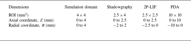An image resolution of ${\sim}2.44$ $\unicode{x03BC}$ m pixel^-1 is achieved with this optical arrangement, whereas the mesh cell size of the refinement zone in the external simulations is 1.2 $\unicode{x03BC}$ m. Further details on instrumentation and optical arrangement can be obtained from Vegad et al. (Reference Vegad2022). Table 2 summarises the regions of interest (ROIs) defined for the hollow-cone spray in the various measurement approaches.

Table 2.

Regions of interest (ROIs) defined for the hollow-cone spray in the different measurement approaches. The origin of coordinates is located at the injector outlet on the central axis, where $Z$ = $R$ = 0 mm.

Figure 3.

(a) Sketch of the test bench comprising the CRSB and the optical arrangement for 2P-LIF. LDM refers to a long-distance microscope, Z denotes the axial direction and R the radial direction. (b) A photograph of the hollow-cone spray highlights the region of interest with a rectangle corresponding to the field used for microscopic shadowgraphy. (c) The spray structure in this dense region is illustrated by an instantaneous shadowgraphy image. The red rectangle in the shadowgraphy image indicates the field of view for 2P-LIF imaging.

3.3.2. Laser-based detection techniques

Surface curvature analysis requires well-defined liquid–gas interfaces. This task becomes more challenging when optically dense regions need to be captured experimentally. Therefore, to identify the most suitable technique, different imaging approaches were evaluated based on the qualitative analysis of the images acquired by each method.

The objective was to image the dense spray in the close vicinity of the injector. The region of interest is marked by a rectangle in the photograph of the n-heptane hollow-cone spray in figure 3(b). In an initial attempt, this dense field was acquired using microscopic shadowgraphy, which provided an overall view of the spray topology near the injector, as illustrated by the instantaneous shadowgraphy image in figure 3(c). This approach allowed the definition of preliminary properties such as spray symmetry, cone angle and break-up distance (Vegad et al. Reference Vegad, Idlahcen, Huang, Cabot, Renou, Duret, Reveillon and Demoulin2024). Shadowgraphy successfully captured liquid–air interfaces at the outer surfaces; in contrast, the inner interfaces were not as clear because the front portion of the hollow-cone spray obstructed the rest. In addition, detached liquid parcels were accompanied by out-of-focus atomising regions. This outcome is expected with this technique, since the signals integrated across the line of sight are collected at each pixel location. As a consequence, post-processing may lead to misinterpretation of the spray structure and, consequently, of the interface curvature. Therefore, a laser-illuminated detection technique, specifically, laser-induced fluorescence (LIF), was selected as the next option. A detailed review of methods to image dense sprays is outside the scope of the present study, but interested readers are referred to the comprehensive review by Linne (Reference Linne2013).

Although Mie scattering is not a good option to illuminate dense sprays, for the sake of comparison with other techniques, planar imaging of the near-field was conducted using both Mie scattering and LIF detection. In the laser-based techniques, the near-field regime at the nozzle exit was captured with a long-distance microscope, achieving a 2.5 $\times$ 2.5 mm $^{2}$ field of view and a 0.2 mm depth of field. The field of view is marked by a red rectangle in the shadowgraph image in figure 3(c). To perform LIF, the first step was to identify a suitable tracer dye for n-heptane fuel. This was accomplished by performing solubility test of different dyes, followed by measurements of the fluorescence characteristics of those that passed the test. Surprisingly, studies on tracers for n-heptane fuel are scarce in the literature. The most familiar tracers of amines (e.g. for water) are fluorescein, eosin and Rhodamine 6G, but none of them is soluble in non-polar alkanes such as n-heptane (Storch et al. Reference Storch, Mishra, Koegl, Kristensson, Will, Zigan and Berrocal2016; Berrocal, Kristensson & Zigan Reference Berrocal, Kristensson and Zigan2018). To dissolve polar or slightly polar tracers (e.g. eosin, Nile red) in non-polar fuels (e.g. n-heptane), one possible approach is to add a small amount of an organic compound such as an alcohol. For example, Durst et al. (Reference Durst, Wensing and Berrocal2018) added 20 % propanol to dissolve eosin Y (60 mg l $^{-1}$ ) in n-heptane. Adding a small percentage of ethanol to a solution of n-heptane and Nile red can shift the maxima of the emission spectrum (Greenspan & Fowler Reference Greenspan and Fowler1985; Durst et al. Reference Durst, Wensing and Berrocal2018). It should be noted that the addition of an organic compound can increase tracer solubility and emission, but also alters fuel properties. However, no organic compound was added during the solubility test of various dyes with n-heptane as the solvent.

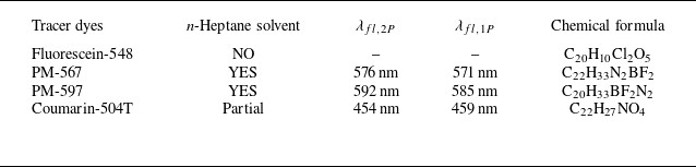
The test was performed for fluorescein-548 (F-548), pyrromethene-597 (PM-597), pyrromethene-567 (PM-567) and coumarin-504T (C-504T). All dyes tested in this study were in the solid phase. A dye concentration of 0.5 % by weight was prepared in n-heptane. Table 3 shows the results of the solubility test. As expected, due to its polar nature, fluorescein-548 was insoluble in n-heptane. Coumarin-504T did not completely dissolve, as some solid particles settled at the bottom of the solution. However, the other two dyes, PM-567 and PM-597, were found to be fully soluble in n-heptane.

Table 3.

Solubility tests and peak emission measurements of various tracer dyes in n-heptane fuel.

Two-photon and one-photon fluorescence characteristics were measured for the soluble dyes. The test was conducted by placing the solution in a quartz cuvette and exciting it with 800 nm and 400 nm laser beams for 2P-LIF and 1P-LIF, respectively. The 400 nm laser light was produced by placing a frequency-doubling crystal in the 800 nm laser light path. The peak fluorescence emissions ( $\lambda _{\!fl}$ ) at both excitations are tabulated in table 3. An emission spectrum of the PM-567 and n-heptane solution is shown in figure 4. To indicate the absorption wavelength in the spectrum, a small fraction of the laser light was directed towards the probe. The emission peaks ( $\lambda _{\!fl,2p}$ ) and ( $\lambda _{\!fl,1p}$ ) were located at ${\sim}576$ and ${\sim}571$ nm, respectively (see figure 4). The theory of two-photon absorption can be found from So et al. (Reference So, Dong, Masters and Berland2000) and Pawlicki et al. (Reference Pawlicki, Collins, Denning and Anderson2009). Based on the solubility test and emission characteristics, PM-567 was selected as the tracer dye for n-heptane fuel.

3.3.3. 2P-LIF

Figure 5 shows instantaneous images of the left half of the n-heptane hollow-cone spray captured using Mie scattering, one-photon laser-induced fluorescence (1P-LIF) and two-photon laser-induced fluorescence (2P-LIF) techniques. As expected, when Mie scattering is applied to a field of continuous liquid sheets and non-spherical liquid structures (as happens in the dense region), the resulting images often contained non-physical artefacts. The direct reflection of the incident laser light at the liquid–air interface of non-spherical structures generated signal intensities strong enough to saturate the camera sensor. However, this was not the case for a fully atomised dispersed phase in the dilute region.

In the case of 1P-LIF, the collected signals shown in figure 5 are a combination of single and multiple scattering events in the surrounding liquid. This occurred because the dye molecule, after excitation, enters a higher energy state in which it emits a photon with sufficient energy to excite nearby molecules. As a result, multiple scattering events propagated into regions outside the laser plane, where they emitted signals at wavelength close to the peak emission. As a consequence, the final images did not exhibit high contrast at the interfaces, as observed at the inner boundary of the liquid sheet in the 1P-LIF image in figure 5.

Figure 4.

Emission spectra of 1P-LIF (dotted line) and 2P-LIF (solid line) for n-heptane fuel with PM-567 tracer dye. The peak emissions of 1P- and 2P-LIF when excited at 400 nm and 800 nm are ${\sim}571$ nm and ${\sim}576$ nm, respectively.

To achieve a clear interface in such an optically dense zone, multiple scattering needed to be reduced by some means. This was accomplished through simultaneous two-photon excitation of dye molecules, whereby the molecules absorb two photons simultaneously. When photons were subsequently emitted after the first scattering, they did not carry sufficient energy to repeat the scattering event. As a result, multiple scattering events were reduced in the 2P-LIF technique, which was capable of delivering high-contrast images (Berrocal et al. Reference Berrocal, Conrad, Püls, Arnold, Wensing, Linne and Miranda2019; Vegad et al. Reference Vegad, Idlahcen, Huang, Cabot, Renou, Duret, Reveillon and Demoulin2024), as shown in figure 5. A total of 500 2P-LIF images, referred to as the image dataset, acquired at 4.4 frames per second were analysed to assess the curvature-based technique.

Figure 5.

Instantaneous images of the left part of the hollow-cone dense spray acquired using Mie scattering, 1P-LIF and 2P-LIF within a 2.5 $\times$ 2.5 mm $^{2}$ field of view, as marked by the red rectangle in the shadowgraphy image of figure 3(c).

4.1. 3-D spray of numerical simulations

In the numerical investigation of atomising sprays, three prevalent approaches exist: (i) deploying a surface plane to track liquid parcels as they traverse this plane within a specific time frame; (ii) using discrete coordinate lines to record the spatiotemporal evolution of liquid parcels (Palanti et al. Reference Palanti, Puggelli, Langone, Andreini, Reveillon, Duret and Demoulin2022); and (iii) extracting the relevant data from every breakup or coalescence event in the simulation (Christensen & Owkes Reference Christensen and Owkes2023). In this study, the first of these strategies is employed to characterise the spray numerically, calculating statistics from data stored at each time step during runtime. For the analysis of 2-D experimental images, it must be however noted that a series of fixed windows is used to sample the curvature of liquid parcels within the field of view. This approach serves as a practical analogue to the surface plane used in the 3-D simulations, allowing curvature-based statistics to be collected despite the dimensional limitation of the experimental images.

Figure 6.

Illustrative representation of the methodology employed to extract physical parameters of the simulated spray through a defined surface plane $S_i$ .

An illustrative overview of the entire procedure is provided in figure 6. A surface plane  $S_i$ is positioned perpendicularly to the streamwise direction, and multiple parameters are recorded on the cell faces of this plane at each discrete time step. As discussed in § 2, the liquid volume fraction $\alpha$ serves as a phase indicator, quantifying the liquid content within each discretised cell. Consequently, the interface normal vector $\boldsymbol{n}_i$ at a given cell face of the surface plane $S_i$ at time $t$ is defined according to

(4.1) \begin{align} \boldsymbol{n}_i = \frac {\boldsymbol{\nabla \!}\alpha }{|\boldsymbol{\nabla \!}\alpha |}. \end{align}

At the designated plane, the curvature $\kappa _i$ is calculated as the divergence of the interface normal vector, defined as

(4.2) \begin{align} \kappa _i^t =-\boldsymbol{\nabla }\boldsymbol{\cdot }\frac {\boldsymbol{\nabla \!}\alpha }{\mid \boldsymbol{\nabla \!}\alpha \mid } .\end{align}

The surface density of the liquid–gas interface, denoted as $\varSigma _i^t$ , is

(4.3) \begin{align} \varSigma _i^t = |\boldsymbol{\nabla \!}\alpha | \end{align}

and the surface interface flux as

(4.4) \begin{align} \varphi \varSigma _i^t = (\boldsymbol{u}_i^t \boldsymbol{\cdot }\boldsymbol{n}) \mid \boldsymbol{\nabla \!}\alpha \mid, \end{align}

where $\boldsymbol{u}_i^t \boldsymbol{\cdot }\boldsymbol{n}$ represents the component of the total gas–liquid mixture velocity that is normal to the plane $S_i$ . Likewise, the flux of the liquid volume fraction is computed according to

(4.5) \begin{align} \varphi \alpha = (\boldsymbol{u}_i^t \boldsymbol{\cdot }\boldsymbol{n}) \alpha. \end{align}

A multitude of parameters are stored at each cell face of the surface $S_i$ , represented as $S_i = f(x_i,y_i,z_i,p_i,\varphi \varSigma _i^t, \varphi \alpha , \kappa _i^t, \boldsymbol{u}_i^t)$ . The coordinates $x_i,y_i,z_i$ specify the cell position, while $p_i$ denotes the face surface area. These parameters collectively serve as the basis for the subsequent characterisation of the spray.

4.2. 2-D spray of experimental images

The details of how a curvature-based technique can be applied to analyse 2-D images of an atomising spray are provided here. High-contrast 2P-LIF image data representing the projected spray field (see § 3.3) are investigated to predict the spray characteristics. It is important to interpret 2P-LIF images from the viewpoint of intensity distribution, ensuring appropriate pre-processing prior to curvature analysis. As mentioned, the curvature-based methodology was originally developed and applied to the 3-D numerical fields, where the full surface geometry is available. In contrast, its application to 2-D spray images requires certain adaptations due to the inherent projection of three-dimensional interfaces onto a planar field of view. These adaptations are also detailed in this section.

The intensity distribution in dense sprays captured via 2P-LIF is analysed herein. Figure 7 shows an instantaneous 2P-LIF image illustrating the distribution of intensities $I_{2P}$ originating from spray structures, with $Z\text{-axial}$ and $R\text{-radial}$ coordinates given in millimetres. A line drawn 0.34 mm from the top intersects the continuous liquid sheet. Variations in $I_{2P}$ along this line are plotted in figure 7 (top-right), showing low intensity levels predominantly in the gaseous regions, which are considered as measurement noise for $I_{2P}\leqslant 10$ .

In the context of the continuous liquid sheet, the interaction between the laser light sheet and both the liquid and gas interfaces is illustrated in the magnified image shown in figure 7 (top-right). Let $A$ and $B$ denote the outer and inner liquid–gas interfaces, respectively, as indicated in the figure, with the laser light sheet propagating from left to right. A pronounced increase in $I_{2P}$ is observed at the outer interface $A$ , whereas a similar trend is not seen at the inner interface $B$ . This discrepancy could be attributed to the nonlinear extinction of laser energy when transitioning from $A$ to $B$ , a phenomenon reported in 2P-LIF imaging by Berrocal et al. (Reference Berrocal, Conrad, Püls, Arnold, Wensing, Linne and Miranda2019). In hollow-cone sprays, the conical liquid sheet obscures the inner interfaces when imaged orthogonally. This portion of the cone, proximal to the laser light sheet plane, undergoes internal reflections and occasional multiple scattering events, emitting signals within the fluorescence band. As a result, $I_{2P}$ gradually transitions from $B$ to $C$ in figure 7. Consequently, intensities in the range $10\lt I_{2P} \leqslant 35$ are attributed to minor multiple scattering events. It is important to note that 2P-LIF significantly reduces multiple scattering, but it cannot entirely eliminate it. Intensities with $I_{2P} \gt 35$ originate from the liquid phase within the laser sheet excitation plane.

Regarding the spray following primary breakup, the variation in intensity along the line located at 1.36 mm from the top is illustrated in the bottom-right graph of figure 7. The liquid–gas interfaces of the liquid parcels exhibit a rapid transition, which can be attributed to the absence of a conical sheet acting as an obstruction. Please note that intensities of the order of $I_{2P} \sim 10$ are considered noise artefacts. Elevated $I_{2P}$ values, including peak emissions, indicate the presence of liquid structures within the illumination plane. Analysis of this intensity distribution informed the selection of appropriate threshold values for subsequent data processing, as detailed in the following sections.

Figure 7.

Analysis of the intensity distribution in a 2P-LIF image of a spray field. Radial intensity profiles ( $I_{2P}$ ) are presented for two axial locations: one at 0.34 mm from the top, intersecting a continuous liquid sheet, and another at 1.36 mm, intersecting detached liquid parcels. A magnified inset illustrates the outer ( $A$ ) and inner ( $B$ ) liquid–gas interfaces, highlighting the effects of internal reflections and minor multiple scattering up to point $C$ within the conical liquid sheet.

Figure 8.

Examination of the 2P-LIF image displayed in figure 7, using varying threshold intensities ( $I_\textit{TR}$ ) for contour mapping.

The primary aim is to filter out noise and intensities arising from multiple scattering events within the proximal liquid sheet near the injector. This is achieved by establishing a threshold intensity ( $I_\textit{TR}$ ) for a given image. To visualise the impact of threshold intensity on the interface, contours of an instantaneous 2P-LIF image (in figure 7) at various threshold values are depicted in figure 8. The Otsu method is recommended for determining $I_\textit{TR}$ , as it effectively distinguishes between the two predominant peaks in the intensity spectrum: noise and peak emission. For this image, the threshold intensity calculated using the Otsu method is $I_\textit{TR}$ = 37, which produces contours closely resembling those of the liquid–gas interface of the original image, as observed in figure 8. Lower threshold values, approximating noise levels (0.5 $\times$ $I_\textit{TR}$ ), tend to overestimate the original structures, whereas higher values approaching peak emission (2 $\times$ $I_\textit{TR}$ ) lead to underestimation. Figure 8 reveals that $I_\textit{TR}$ primarily affects the continuous liquid sheet from the injector rather than isolated structures, mainly due to contributions from internal scattering in the continuous region. Therefore, the influence of threshold intensity on the continuous spray increases with increasing sheet breakup distance, an effect that becomes more pronounced at lower flow rates. However, under the optimal operating pressure and mass flow conditions considered for the atomiser in the present work, liquid sheet breakup occurs very close to the injector. Consequently, the threshold intensity $I_\textit{TR}$ determined under these operating conditions is employed in the subsequent data analysis, as detailed in the following sections.

5.1. Equivalent Sauter mean diameter

The spray evolution from the injector outlet to the formation of liquid parcels in the external domain of numerical simulations is analysed by computing the equivalent Sauter mean diameter (eSMD or $l_{32}$ ) at successive stages. It should now be noted that the derivation of $l_{32}$ is carried out from the analysis of the initial spray, where most non-spherical liquid structures are present. However, this requires a precise definition of the Sauter mean diameter (SMD) as it pertains to spherical droplets in dispersed sprays. In this context, the PDA technique was employed in previous work (Vegad et al. Reference Vegad, Idlahcen, Huang, Cabot, Renou, Duret, Reveillon and Demoulin2024) to size droplets in such dispersed regions. The Sauter mean diameter $D_{32}$ is defined as the ratio of the total droplet volume ( $V_l$ ) to the total droplet surface area ( $A_l$ ), as (Lefebvre & McDonell Reference Lefebvre and McDonell2017)

(5.1) \begin{align} D_{32}^{\textit{PDA}} = \frac {\sum _i N_i D_i^3}{\sum _i N_i D_i^2} \approx 6\frac {V_l}{A_l}, \end{align}

where $i$ denotes the drop-size class, $N_i$ is the number of droplets within this class and $D_i$ is the midpoint diameter of the class.

The liquid volume fraction $\alpha$ is employed to define the equivalent Sauter mean diameter ( $l_{32}$ ) for all structures present in the initial spray obtained from numerical simulations. We recall that $\alpha$ ranges from $0$ (for gas) to $1$ (for liquid). This concept, together with (5.1), yields an expression for $l_{32}(V)$ applicable to any given control volume, as given by

(5.2) \begin{align} l_{32}(V) = 6 \frac {\iiint _{V}\alpha \,{\rm d}v}{\iiint _{V} \mid \boldsymbol{\nabla \!}\alpha \mid \,{\rm d}v}, \end{align}

where ${\rm d}v$ is an elemental volume. Equation (5.2) gives a preliminary estimation of $l_{32}(V)$ by integrating the liquid content within each cell of the considered spray in numerical simulations. This formulation is more general than (5.1), as it can determine the equivalent Sauter mean diameter $l_{32}(V)$ for non-spherical liquid structures, while also recovering the conventional SMD for sprays composed solely of spherical droplets. The constant 6 in (5.1) and (5.2) originates from the geometric relation between the volume and surface area of a sphere, $V_i/A_i = D_i/6$ , ensuring that the equivalent Sauter mean diameter $l_{32}$ is dimensionally consistent with the classical definition of $D_{32}$ . Accordingly, $l_{32}$ would recover the conventional $D_{32}$ if the droplets were perfectly spherical.

An alternative approach to calculate $l_{32}$ is through the concept of surface flux. If the variables of liquid structures crossing a surface plane $S$ (as illustrated in figure 6) are recorded over a time interval $T$ in numerical simulations, then $l_{32}(S)$ can be evaluated using

(5.3) \begin{align} l_{32}(S) = 6\frac {\int _{T} \iint _{S}(\alpha \boldsymbol{u} \boldsymbol{\cdot }\boldsymbol{n} \,{\rm d}s) \,{\rm d}t}{\int _{T} \iint _{S}(\varSigma \boldsymbol{u} \boldsymbol{\cdot }\boldsymbol{n}\, {\rm d}s) \,{\rm d}t}. \end{align}

Following this approach, the evolution of the atomisation process is examined by evaluating $l_{32}(S)$ at different streamwise locations within the external simulation domain. Several horizontal measurement planes are positioned in the refinement zone (up to 1.3 mm) of the numerical domain to compute the volume fraction flux $\varphi \alpha = (\boldsymbol{u} \boldsymbol{\cdot }\boldsymbol{n})\alpha$ and the surface interface flux $\varphi \varSigma = (\boldsymbol{u} \boldsymbol{\cdot }\boldsymbol{n})|\boldsymbol{\nabla \!}\alpha |$ of the liquid crossing them. Surface integration of these fluxes over the total computation time provides the total liquid volume and total liquid surface area across each plane. These quantities are then used to evaluate $l_{32}(S)$ according to (5.3).

Figure 9.

Evolution of $l_{32}(S)$ along the axial coordinate $Z$ in the simulation domain, with the dotted horizontal line marking the value of $l_{32}(S)$ calculated for the stable zone.

The resulting $l_{32}(S)$ values at the axially located measurement planes in the simulation domain are plotted in figure 9. The highest value is observed at the injector outlet, corresponding to the flat liquid sheet. The sharp reduction of $l_{32}(S)$ up to $Z = 0.2$ mm cannot be unequivocally attributed to the preliminary breakup of the film, as it may instead reflect an increase in the interfacial surface area caused by the wrinkling and stretching of the liquid–gas interface. This behaviour denotes the onset of liquid sheet destabilisation, associated with the growth of interfacial corrugations and the formation of surface protrusions. At this stage, the liquid core remains essentially continuous, consistent with the experimental observations from 2P-LIF imaging. Beyond this point, however, $l_{32}(S)$ progressively increases along the streamwise direction within the refinement zone. This trend may be linked to the formation and convective transport of small droplets that deviate from the nominal spray cone angle, leading to a partial loss of liquid structures outside the refined region. As a consequence, the liquid volume fraction diffuses in such a way that the liquid–gas interface cannot be fully captured in the non-refined region.

From $Z = 1$ mm onwards, the magnitude of $l_{32}(S)$ converges towards a stable value, which is maintained up to the end of the refinement zone ( $Z = 1.3$ mm). The increase in $l_{32}(S)$ of the two last points in figure 9 is attributed to the end of the refined region, with a significantly larger cell size. The asymptotic value within the refined region, $l_{32}(S)\sim 27.48$ $\unicode{x03BC}$ m, is represented by a horizontal dotted line in figure 9. This value is in close agreement with the droplet Sauter mean diameter measured by PDA, $D_{32}^{\textit{PDA}} = 28$ $\unicode{x03BC}$ m, at an axial distance of $Z = 3$ mm. At this location, the PDA measurements exhibit a Doppler burst validation of ${\geqslant }90\,\%$ , ensuring reliable experimental statistics. This comparison is intended to demonstrate that the curvature-based methodology can capture the equivalent Sauter mean diameter $l_{32}(S)$ of spray structures within the stable zone ( $Z\geq 1$ mm), even though the PDA measurement is taken further downstream.

Therefore, it is appropriate to define the measurement plane downstream of the primary breakup ( $Z \gt 0.2$ mm) and within the stable region of the refinement zone. The selected measurement plane is then set at the axial location $Z = 1.2$ where the different variables discussed in § 4.1 are stored. This location is chosen as it is sufficiently far from the initial breakup region, while still lying within the refined zone, ensuring reliable characterisation of the spray.

5.2. Equivalent surface mean diameter from images

In the 2P-LIF technique, a hollow-cone spray illuminated by a laser light sheet is captured with the camera placed orthogonally, yielding 2-D projected images of the spray. Extracting parameters from such 2-D images is inherently more challenging than from a 3-D numerical field, as not all information required for the calculation of spray characteristics is accessible. Consequently, methods suitable for 3-D simulations, such as the surface plane approach (refer to § 4.1), cannot be directly applied, since liquid structures in the images do not exhibit three-dimensional surfaces. Instead, a level-set-based approach is employed, as explained next.

The position of liquid structures (or more specifically, their interfaces) within the gaseous medium is obtained by defining a distance function ( $\phi$ ). This function is computed using an algorithm based on k-dimensional trees (Maneewongvatana & Mount Reference Maneewongvatana and Mount2002), employing the sliding midpoint rule for nearest-neighbour searches. The sign of the distance (i.e. the level-set) between a point in the domain and the nearest point on the interface is positive if the point lies in the liquid phase or negative if it lies in the gaseous phase. The distance function for the 2P-LIF image (figure 7) is illustrated in figure 10(a). It is further used to define the projected phase indicator ( $\textit{ppi}$ ), as shown in figure 10(b), with $\textit{ppi}$ calculated as $ppi = (1+\tanh {(2\phi ))}/2$ . In this definition, $ppi = 1$ corresponds to the liquid phase, $ppi = 0$ to the gaseous phase and intermediate values indicate the transition across interfaces. In addition, to avoid sharp edges at the perimeters of some liquid structures, a tangential interpolation is applied to smooth the interface. This operation prevents the curvature from becoming infinite at sharp edges, effectively neglecting very small droplets in the subsequent predictions. In particular, the present study considers the smallest diameter that can be reliably captured in 2P-LIF as 2 $\times$ 2 pixel $^2$ , corresponding to 4.8 $\unicode{x03BC}$ m.

It should be noted that the $\textit{ppi}$ field is introduced primarily to smooth the liquid–gas interface and to enable the evaluation of curvature-related quantities in a continuous and differentiable manner. The thresholded 2P-LIF images present sharp discontinuities at the liquid boundaries, which can lead to infinite or numerically unstable curvature estimates. By applying the $\textit{ppi}$ field, these discontinuities are removed, resulting in smoother interfaces suitable for subsequent geometrical analysis. Nevertheless, for integral quantities such as the surface mean diameter ( $l_{21}$ ), the thresholded binary images can also be directly employed, since curvature information is not required for their computation. Further discussion on this aspect in the context of size distribution is provided in § 7.

Figure 10.

(a) Instantaneous level-set 2-D field (distance function) calculated from the 2P-LIF image and (b) projected phase indicator ( $\textit{ppi}$ ) derived from this function. The regions used for evaluation are highlighted with boxes.

Figure 11.

Equivalent surface mean droplet diameter $l_{21}(S)$ obtained from a time-averaged 2P-LIF dataset of 500 images applying (5.4) to 0.12 $\times$ 2.5 mm $^2$ windows at consecutive axial locations from the injector outlet. The dashed line at $l_{21}$ = 30.5 $\rm \unicode{x03BC} m$ represents the value calculated over the complete stable zone.

The $\textit{ppi}$ field of 2P-LIF images is analogous to the $\alpha$ field of a 3-D simulated spray. A key is that a 3-D cell in the numerical domain represents a control volume containing a certain liquid volume fraction ( $\alpha$ ), whereas a 2-D pixel in an image indicates the projected liquid flux. Consequently, unlike the equivalent Sauter mean diameter ( $l_{32}$ ) calculated from 3-D simulations, we computed the equivalent surface mean diameter ( $l_{21}$ ) from the 2P-LIF images. One could argue that, if signals collected in LIF were integrated over the liquid volume within the laser plane and combined with surface area measurements from Mie scattering, the resulting LIF/Mie ratio could be used to estimate $l_{32}$ . However, for such a complex and dense spray, this ratio is difficult to obtain, and simultaneous Mie figures were not captured in the present study. Therefore, the evolution of the spray is characterised through $l_{21}(S)$ , as

(5.4) \begin{align} l_{21}(S)=4 \frac {\iint _{S} ppi \,{\rm d}s}{\iint _{S} \mid \boldsymbol{\nabla \!}ppi\mid\, {\rm d}s}, \end{align}

where ${\rm d}s$ is the elemental area. Equation (5.4) is derived based on the definition of the area mean diameter ( $D_{21}$ ) for spherical droplets, given by

(5.5) \begin{align} D_{21}^{\textit{PDA}} = \frac {\sum _i N_i D_i^2}{\sum _i N_i D_i} \approx 4\frac {A_l}{P_l}, \end{align}

where $P_l$ denotes the perimeter of the droplets.

Equation (5.4) is applied to 0.12 $\times$ 2.5 mm $^2$ (or 50 $\times$ 1024 pixels $^2$ ) consecutive windows along the axial direction. The resulting $l_{21}(S)$ for each window is time-averaged over a dataset of 500 2P-LIF images, which ensures statistical convergence in the stable zone. The time-averaged values are plotted in figure 11. For simplicity, an early stage of atomisation process considered in the present study is divided into four regions: region 1, where the continuous liquid sheet is always present; region 2, in which detached liquid parcels experience interfacial instabilities and break up into ligaments; region 3, an evolving zone; and region 4, where non-spherical structures undergo further morphological change and momentum breakup. These four regions are marked in figure 10(b).

Note that the injector outlet is located about 0.058 mm (or 24 pixels) from the top. Therefore, the initial part of the first window contains no liquid and the first point in figure 11 appears lower before reaching the peak value of $l_{21}(S)$ . However, as expected, $l_{21}(S)$ is higher in region 1 due to the continuous liquid stream. A steep decrease in $l_{21}(S)$ in region 2 corresponds to the primary breakup into large liquid filaments, which continue to break up into ligaments. In region 3, ligament-like structures do not undergo multiple breakup events, resulting in a gradual decrease of $l_{21}(S)$ . From region 3 onwards, the $l_{21}(S)$ becomes almost stable (region 4), which is therefore referred to as the stable zone.

The horizontal line in figure 11 marks $l_{21}$ = 30.5 $\unicode{x03BC}$ m, calculated for the entire stable zone. In this near-field regime, the Doppler bust validation is recorded as approximately 70 % at $Z$ = $R$ = 2 mm in PDA measurements.

It is worth noting that the onset of the stable region appears slightly earlier in the numerical simulations (around 1.0 mm, recall figure 9) than in the experiments (around 1.5 mm, as seen in figure 11). This difference arises mainly from the distinct nature and resolution of both datasets. In the simulations, several axial planes separated by 0.05 mm were analysed, providing high spatial resolution in the evaluation of $l_{32}$ . In contrast, the experimental 2P-LIF images were processed using 0.12 $\times$ 2.5 mm $^2$ axial boxes to ensure statistical convergence, which leads to a smoother and slightly delayed evolution of $l_{21}$ . Furthermore, while the numerical data are fully three-dimensional, the experimental data represent pseudo-2-D projections of the liquid structures, which can also contribute to a downstream shift of the stable region.

Figure 12.

(a) Surface curvature distribution (SCD) at the 1.2 mm axial location in the refinement zone. The dashed line is the lower cut-off value of the curvature ( $\kappa _{\textit{Num,min}}$ ). (b) Iso-contours with curvature values ranging from negative to positive in the numerical simulation.

6.1. Surface curvature distribution of 3-D simulated spray

A relationship between surface ( $S$ ) and curvature of simulated spray ( $\kappa _{\textit{Num}}$ ) is described through the surface curvature distribution (SCD) shown in figure 12(a). The measurement plane is located at $Z$ = 1.2 mm within the refinement zone of the numerical domain. The curvature is defined as the divergence of the normal vector at the interface, and computed using (4.2) as $\kappa _{\textit{Num}} = -\boldsymbol{\nabla }\boldsymbol{\cdot }\boldsymbol{n}$ , where $\boldsymbol{n}$ is the normal vector at the given cell face of the surface plane. Note that negative curvatures in the plot physically correspond to bubbles and concave liquid structures. Therefore, a fundamental step of this approach is to eliminate surfaces with negative curvatures, as they do not contribute to the final drop size distribution. The iso-contours of negative curvature ( $\kappa _{\textit{Num}}\lt 0$ ) of concave shape are displayed in figure 12(b). Most of these surfaces eventually evolve into positive curvatures ( $\kappa _{\textit{Num}}\gt 0$ ) of convex shapes as they develop to near-spherical shapes downstream.

Once the curvature values are obtained in the stable zone (region 4), near-zero (very small) curvatures are still present in the SCD (figure 12 a). These originate from nearly flat elements. Such small curvatures would generate unrealistically large droplets if the SCD were converted directly into a droplet size distribution. These large drops are non-physical, as they correspond to flat surfaces, and should thus be excluded from the droplet size distribution. However, the question arises: up to what extent? To resolve this, (5.2) is referenced, which is used to compute the equivalent ‘flux-based’ SMD, $l_{32}(S)$ , for a stable zone (i.e. when $l_{32}(S)$ has converged). Then, $D_{32}^{Num}$ is calculated from the droplet size distribution by disregarding large droplets until $D_{32}^{Num} \approx l_{32}(S)$ . The lower cutoff value ( $\kappa _{\textit{Num,min}}$ ) of the curvature distribution in figure 12(a) is set using this maximum diameter, $\kappa _{\textit{Num,min}}=4/l_{32}(S)$ , and is indicated by a dashed line in the figure. Therefore, curvatures below this threshold are not considered in the final size distribution either.

6.2. Length curvature distribution of 2-D experimental spray

The evolution of curvatures in an atomising spray captured by 2P-LIF imaging can be characterised using the perimeter length ( $P_{l,L}$ ) of the liquid structures and their corresponding curvatures ( $\kappa _{2P\text{-}\textit{LIF}}$ ). Recall that the curvatures of projected liquid structures in 2-D images are calculated as the divergence of the normal vector at the interface, given by $\kappa _{2P\text{-}\textit{LIF}}$ $=$ $-\boldsymbol{\nabla }\boldsymbol{\cdot}$ $(\boldsymbol{\nabla }\phi /|\boldsymbol{\nabla }\phi |)$ , where the normal vector is obtained from the gradient of the distance function ( $\phi$ ) across the interface. The perimeter length is defined as the norm of the gradient of the $\textit{ppi}$ field. Figure 13 presents the $P_{l,L}{-}\kappa _{2P\text{-}\textit{LIF}}$ distribution, or length curvature distribution (LCD) collected over 500 2P-LIF images for regions 1–4 at different axial locations (as defined in § 5.2). The LCD is obtained by weighting the curvature distribution with the corresponding perimeter length. The vertical line in figure 13 denotes zero curvature. Region 1 is physically expected to display the highest number of perimeter lengths with near-zero curvature because the continuous liquid stream is largely flat. In addition, initial disturbances originating from the internal geometry of the atomiser create an alternating crest- and trough-like wavy pattern in the continuous liquid sheet of region 1. These periodic concave and convex shapes yield an approximately equal number of negative and positive curvatures, as evidenced by the near symmetry of the LCD plot for region 1 compared with the other regions in figure 13. It must be noted that the distorted shape of the LCD plot for this region is likely due to the limited number of curvatures away from zero caused by the predominance of large, flat, wavy liquid structures in the continuous film, reflecting the local morphology of the spray.

Region 2 shows the LCD peak shifted towards positive curvatures, indicating that most detached liquid parcels exhibit convex surfaces (figure 13). The near-zero peak in this region reflects the presence of relatively large, almost flat liquid parcels. Additionally, the total perimeter length associated to negative curvatures is higher in region 2 than in regions 3 and 4. This could be attributed to local instabilities of liquid parcels immediately after detachment from the continuous stream. These instabilities gradually diminish as larger liquid packages break up into ligaments. Most of these ligaments have positive curvatures and evolve towards spherical shapes, which is confirmed by the rightward-shifted LCD peaks in regions 3 and 4 (figure 13). This shift also reflects the breakup of ligaments into smaller liquid structures. Overall, figure 13 demonstrates that as we move from region 1 to region 4, liquid structures increasingly adopt positive curvatures and tend towards spherical droplets. This evolution can be further analysed by examining the percentage of positive-curvature structures along the streamwise direction.

Figure 13.

Perimeter length curvature distribution (LCD) collected over 500 images of the atomising spray in regions 1–4, as marked in figure 10(b).

An atomising spray continuously changes its morphology before reaching the final stage, where the aim is to form the final droplets. This morphological evolution of the spray is tracked through curvature distribution and thus helps identify the stages of the atomisation process. Figure 14 shows the percentage of positive-curvature perimeter length ( $P_{l,L}$ ) of liquid structures at successive stages, which increases along the axial distance as atomisation progresses. Here, $P_{l,L}$ is the ratio of perimeter lengths with positive curvatures to the total of positive and negative curvatures. At the injector outlet, approximately 50 $\,\%$ of the length corresponds to positive curvature, indicating that the continuous liquid sheet is not completely flat, but exhibits some wavy shape. After the first detachment of liquid parcels into large structures, some surface morphologies still have negative curvature. However, approximately $80 \,\%$ of positive-curvature perimeter lengths are observed in the ligament zone (region 3), occurring within an axial distance of 0.5–1.5 mm. In the stable zone (region 4), these surfaces retain their curvature and slightly more positive curvatures are collected as the spray advances in the streamwise direction. Consequently, the majority of these curvatures are expected to produce spherical droplets. At this stage, since the positive-curvature perimeter length is more than $80 \,\%$ , the atomisation process is considered nearly complete.

Figure 14.

Percentage of positive-curvature perimeter length ( $P_{l,L}$ ), extracted during the evolution of liquid structures along the streamwise direction within the marked regions 1–4 of the 2P-LIF image data.

7.1. DSD of 3-D simulated spray

In numerical simulations, the curvature $\kappa _{\textit{Num}} = -\boldsymbol{\nabla }\boldsymbol{\cdot }(\boldsymbol{\nabla \!}\alpha /|\boldsymbol{\nabla \!}\alpha | )$ is stored at the cell faces on the measurement plane ( $Z$ = 1.2 mm) at each computational time step (8 $\times$ 10 $^{-10}$ s) and used to calculate the droplet diameter, $D_\kappa ^{Num}=4/\kappa _{\textit{Num}}$ . It is to be noted that the entire surface accumulated during the computation time is considered for extracting the curvature statistics. The total integrated time of 0.1 ms is considered to minimise statistical error in the curvature-based droplet size estimation. The number of droplets that could be produced from the surfaces passing through the measurement plane is given by the ratio $n_\kappa ^{Num} = S_\kappa /\pi (D_k^{Num})^2$ . Hence, the drop size distribution in numerical simulations ( $\textit{DSD}^{Num}$ ) characterised at the measurement plane is presented in figure 15. The contribution of negative and zero curvatures is not taken into account in the distribution. Likewise, near-zero curvatures (from almost flat elements) are also discarded with reference to $l_{32}(S)$ considering data belong to regions 3 and 4, as explained in § 6. In figure 15, the peak of the $\textit{DSD}^{Num}$ curve is 17 $\unicode{x03BC}$ m and the Sauter mean diameter calculated using droplet size and number information in (5.1) is $D_{32}^{Num}$ = 27.5 mm.

The simulated $\textit{DSD}^{Num}$ is compared with $\textit{DSD}^{\textit{PDA}}$ obtained from PDA measurements at different axial ( $Z$ ) and radial ( $R$ ) locations. Since the simulated spray cone angle is similar to that of hollow-cone spray of the given atomiser, the PDA measurements taken along the spray cone angle (at equal $Z$ and $R$ locations) are considered for comparison. Furthermore, the Doppler bust validation in PDA measurements near the spray injection at $Z$ = $R$ = 1 and 2 mm is approximately 50 % and 70 %, respectively (Vegad et al. Reference Vegad, Idlahcen, Huang, Cabot, Renou, Duret, Reveillon and Demoulin2024; Sun et al. Reference Sun, Vegad, Li, Dreßler, Renou, Nishad, Demoulin, Hasse and Sadiki2024), while the validation is $\geqslant 90\,\%$ at $Z$ = $R$ = 3 mm onwards.

In figure 15 (left), although the Doppler bust validation in the PDA measurements at $Z = R = 2$ mm is relatively low, the simulated $\textit{DSD}^{Num}$ is still compared with the measured $\textit{DSD}^{\textit{PDA}}$ at this location. The size distributions show poor agreement in this case. However, a favourable agreement is obtained when the predicted $\textit{DSD}^{Num}$ at $Z = R = 1.2$ mm in the simulation domain is contrasted with the measurements at $Z = R = 3$ mm, as shown in figure 15 (middle). In this case, the peak of the prediction curve is shifted towards larger diameters, indicating a higher presence of large drops compared with those observed in the PDA data, while the number of tiny droplets is underpredicted in $\textit{DSD}^{Num}$ . This discrepancy can be understood by recalling that the eSMD or $l_{32}(S)$ , calculated in successive measurement planes starting from the injector outlet (figure 9), increases from 0.2 mm up to 1.2 mm. This behaviour arises because tiny droplets move away from the spray cone. As a result, their contribution is underestimated at the measurement plane located in the stable zone, further downstream of the injector. Consequently, when comparing SMD values (figure 15), the simulation tends to predict slightly larger sizes, i.e. $D_{32}^{Num} \gt D_{32}^{\textit{PDA}}$ . At $Z$ = $R$ = 4 mm, $D_{32}^{Num}$ remains of the same order of magnitude as $D_{32}^{\textit{PDA}}$ , although the measured $\textit{DSD}^{\textit{PDA}}$ exhibits a comparatively broader span. Similarly, when $\textit{DSD}^{Num}$ is compared with PDA measurements at further downstream locations, both the span of $\textit{DSD}^{\textit{PDA}}$ and the measured $D_{32}^{\textit{PDA}}$ remain consistently larger than the estimated values from the simulations.

Figure 15.

Drop size distribution from numerical simulations ( $\textit{DSD}^{Num}$ ) estimated at $Z$ = $R$ = 1.2 mm in the numerical domain is compared with the distributions obtained from PDA measurements ( $\textit{DSD}^{\textit{PDA}}$ ) at $Z$ = $R$ = 2, 3 and 4 mm. The Sauter mean diameters calculated from these distributions using (5.1) are also shown.

In summary, the surface curvature information collected at $Z$ = $R$ = 1.2 mm in the simulation domain is able to provide a good average approximation, based on the $D_{32}$ comparison, of the drop size distribution observed in experimental PDA measurements at $Z$ = $R$ = 3 mm. This suggests that, when properly located, the surface curvature distribution obtained at an early stage of atomisation (defined in § 1) can provide valuable insight into the downstream drop size distribution.

7.2. DSD of 2-D experimental spray

It is now appropriate to describe the final results of the 2P-LIF image data analysis. The curvature of the liquid structures in the 2-D images is defined as $\kappa _{2P\text{-}\textit{LIF}} = -\boldsymbol{\nabla }\boldsymbol{\cdot }(\boldsymbol{\nabla }\phi /|\boldsymbol{\nabla }\phi |)$ , and the corresponding droplet diameter is given by $D_{k}^{2P\text{-}\textit{LIF}}=2/\kappa _{2P\text{-}\textit{LIF}}$ . Accordingly, the number of droplets that can be derived from the local perimeter length is calculated as $n_{\kappa }^{2P\text{-}\textit{LIF}}=|\boldsymbol{\nabla \!}ppi|/\pi D_{k}^{2P\text{-}\textit{LIF}}$ . To provide an overall idea of the contribution of all types of early spray curvatures (negative, zero and positive), a raw drop size distribution reconstructed from the curvatures and their perimeters is plotted in figure 16. In region 1, a large number of both positive and negative ‘diameters’ is observed, owing to the numerous positive and negative curvatures (convex and concave shapes) associated with the wavy liquid sheet. After the primary breakup of this continuous sheet into large liquid parcels in region 2, the occurrence of concave surfaces (negative curvature) is higher than further downstream due to the persistence of local interfacial instabilities. Consequently, figure 16 shows larger negative diameters in region 2 compared with regions 3 and 4. These negative curvatures arise from stretching and contraction after the primary breakup. The negative diameters shown in figure 16 are included only for demonstration purposes and are entirely excluded from the size distribution comparison. A considerable amount of small positive diameters is also detected in region 2, which could mainly originate from experimental artefacts, although some contribution from satellite droplets generated by pinching mechanisms cannot be ruled out.

Figure 16.

Droplet size distribution ( $\textit{DSD}^{2P\text{-}\textit{LIF}}$ ) reconstructed from positive and negative curvatures (see $P_{l,L}{-}\kappa _{2P\text{-}\textit{LIF}}$ distribution in figure 13) for the continuous spray as well as for detached ligaments and droplets structures in the image dataset.

Figure 17.

Comparison between drop size distribution ( $\textit{DSD}^{2P\text{-}\textit{LIF}}$ ) obtained from the 2P-LIF analysis in region 4 (within a 1 $\times$ 2.5 mm $^2$ window at $Z$ = 1.5 mm) and that measured with the PDA technique ( $\textit{DSD}^{\textit{PDA}}$ ). The area mean diameter calculated using (5.5) for each distribution is marked with vertical lines.

Region 3 and region 4 consist mainly of ligaments with maximum curvature recovery, leading to a typical size distribution. Moreover, most of the curvatures remained positive while travelling from region 3 to region 4 (figure 14). This trend is reflected in the size distributions, where the peaks of $\textit{DSD}^{2P\text{-}\textit{LIF}}$ are comparable for both cases (see the curves of region 3 and region 4 for positive diameters in figure 16). The slightly broader distribution in region 3, which narrows in region 4, provides further insight into how ligaments evolve towards a stable spherical shape. For this reason, region 4 has been considered as an atomising stage, believed to be representative of the droplet sizes produced further downstream. A more detailed characterisation of this stage, including size prediction and comparison with experimental measurements, is now given.

The drop size approximated from the 2P-LIF analysis (specifically from region 4, i.e. the stable zone) is compared with direct PDA measurements in figure 17. The lower bound of the $\textit{DSD}^{2P\text{-}\textit{LIF}}$ in the stable zone starts at 4.8 $\unicode{x03BC}$ m, since 2 $\times$ 2 pixel $^{2}$ is assumed to be the smallest droplet captured in 2P-LIF. In contrast, the upper bound can, in principle, be infinite due to flat surfaces (zero curvature). Therefore, similar to the case of the simulated $\textit{DSD}^{Num}$ , the upper end of the estimated $\textit{DSD}^{2P\text{-}\textit{LIF}}$ from 2P-LIF is limited by defining a minimum curvature with the help of $l_{21}(S)$ , given as $\kappa _{2P\text{-}\textit{LIF,min}}=2/l_{32}(S)$ . The resulting distribution is then compared with $\textit{DSD}^{\textit{PDA}}$ measured at different spatial locations downstream of the atomiser.

In figure 17, the $\textit{DSD}^{2P\text{-}\textit{LIF}}$ obtained from the curvature distribution of the liquid spray in region 4 of 2P-LIF is compared with $\textit{DSD}^{\textit{PDA}}$ measured in PDA at $Z$ = $R$ = 2–6 mm, as well as with integrated measurements for $R$ = 3–5 mm at $Z$ = 4 mm. The plots clearly show that the estimated $\textit{DSD}^{2P\text{-}\textit{LIF}}$ becomes progressively more consistent with $\textit{DSD}^{\textit{PDA}}$ when moving from $Z = R = 2$ mm towards downstream locations. A reasonable agreement between the peaks of both distributions is observed at $Z$ = $R$ = 3 mm, though with a slight deviation in their $D_{21}$ . Interestingly, the closest match of the estimated size distribution is achieved with the PDA measurement at $Z$ = $R$ = 4 mm. A small fraction of large droplets is still predicted from the 2P-LIF analysis. One possible reason is the actual presence of a few large droplets that undergo secondary breakup further downstream. Another qualitative explanation, based on the physics of the atomisation process and the data acquisition methods, is that certain morphological changes create instantaneous local almost-flat surfaces. In these regions, the curvature values are small, which can lead to artificially large droplets in the reconstructed size distribution.

The discrepancies between $\textit{DSD}^{\textit{PDA}}$ and $\textit{DSD}^{2P\text{-}\textit{LIF}}$ can also be attributed to the intrinsic methodological differences between both diagnostics. While PDA measurements reliably detect nearly spherical droplets (validated above 90 % beyond a radial distance of 3 mm), the 2P-LIF curvature-based approach provides a two-dimensional curvature field that may include irregular or transient liquid structures. The comparison at $Z$ = 1.5 mm (2P-LIF) and $Z$ = $R$ = 4 mm (PDA) therefore reflects distinct but complementary regions of the atomisation process: the former still containing non-spherical liquid structures and the latter corresponding to a nearly spherical droplet field. This methodological distinction is considered when identifying the best matching location between both datasets, as discussed now.

To verify that $Z$ = $R$ = 4 mm is indeed the spatial location where the best agreement is achieved, further comparisons are made between the estimated $\textit{DSD}^{2P\text{-}\textit{LIF}}$ and $\textit{DSD}^{\textit{PDA}}$ measured at downstream locations, namely $Z$ = $R$ = 5 and 6 mm, as shown in figure 17. For both PDA measurements, the distribution peaks are shifted towards large diameters compared with the estimated one. Since the most favourable agreement is obtained at $Z$ = $R$ = 4 mm, an additional comparison was performed by integrating PDA measurements over radial locations of $\pm$ 1 mm around this point. This integration, corresponding to droplets measured at $R$ = 3–5 mm at $Z$ = 4 mm from the atomiser, is also presented in figure 17. However, the outcome of this comparison shows that the agreement of the estimated size distribution with the integrated PDA measurements remains unsatisfactory. A possible explanation is that, further downstream, the spray undergoes stronger radial dispersion of droplets, broadening the measured distribution. Such enhanced spreading in the PDA data may account for the deviation from the more localised drop size distribution obtained from 2P-LIF.

Figure 18.

Comparison of drop size distributions estimated from curvature analysis of the simulated spray ( $\textit{DSD}^{Num}$ ) and the 2P-LIF images ( $\textit{DSD}^{2P\text{-}\textit{LIF}}$ ), together with those measured by PDA ( $\textit{DSD}^{\textit{PDA}}$ ). The Sauter mean diameters ( $D_{32}$ ) are calculated from each distribution using (5.1).

Therefore, based on the previous discussion, the $\textit{DSD}^{2P\text{-}\textit{LIF}}$ estimated from the 2P-LIF curvature distribution at $Z$ = 1.5 mm downstream of the nozzle shows the closest agreement with $\textit{DSD}^{\textit{PDA}}$ measured at $Z$ = $R$ = 4 mm. This indicates that the spray is being characterised in terms of drop size distribution in region 4, which corresponds to a more advanced stage of the atomisation process: liquid structures are largely detached but not yet fully spherical. Most of the atomisation is completed in this stable zone, and the spray structures present are sufficiently representative to define the surface mean diameter and, on average, the overall spray characteristics. Although the present validation is limited to this specific operating condition, the methodology itself is applicable to other spray conditions and fragmentation scenarios, provided appropriate imaging or simulation data are available.

A global comparison among the drop size distributions estimated from the numerical simulation at $Z$ = 1.2 mm and from the 2P-LIF image analysis in region 4 at $Z$ = 1.5 mm is presented in figure 18. As expected, the $\textit{DSD}^{2P\text{-}\textit{LIF}}$ is broader than the $\textit{DSD}^{Num}$ because the curvature information extracted from the 2P-LIF images corresponds to a 1 mm-wide window (region 4), whereas in the simulation it is obtained at a single measurement plane. Moreover, the fraction of larger droplets is higher in the $\textit{DSD}^{2P\text{-}\textit{LIF}}$ , which can be attributed to the lower bound of curvatures captured experimentally, $\kappa _{2P\text{-}\textit{LIF,min}}\lt \kappa _{\textit{Num,min}}$ . This difference is reflected in the SMDs calculated from both distributions using (5.1), resulting in $D_{32}^{2P\text{-}\textit{LIF}}\gt D_{32}^{Num}$ , as shown in figure 18.

Both estimated distributions are also compared with the direct PDA measurements. The closest PDA measurement location where the Doppler bust validation exceeds 90 % ( $Z = 3$ mm) is used for this comparison. At this axial position, most of the liquid structures have evolved into nearly spherical droplets, resulting in smaller measured diameters. Consequently, the SMD obtained from PDA is the smallest, and the global relation established from the analysis presented in this study is $D_{32}^{2P\text{-}\textit{LIF}}\gt D_{32}^{Num}\gt D_{32}^{\textit{PDA}}$ .