


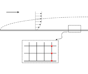



1. Introduction
The fast and accurate prediction of skin friction  $c_f$ and wall heat flux
 $q_w$ is a critical issue in the aerodynamic/aerothermal numerical simulation of hypersonic vehicles. The velocity and temperature in hypersonic boundary layers vary sharply near the wall, which brings great difficulties in predicting
 $c_f$ and
 $q_w$ accurately. Available studies (Hoffmann, Siddiqui & Chiang Reference Hoffmann, Siddiqui and Chiang2013; Thivet, Besbes & Knight Reference Thivet, Besbes and Knight2013) have shown that simulation results for
 $c_f$ and
 $q_w$ are highly sensitive to the distribution of grid points near the wall, especially the distance of the first grid point off the wall
 $\Delta y_1$. To calculate accurately
 $c_f$ and
 $q_w$ of a hypersonic vehicle,
 $\Delta y_1$ needs to be very small, generally
 $10^{-6}$ m or even smaller, which brings a huge computational consumption. For three-dimensional complicated configurations, the numerical integration time step is limited greatly by the dense mesh, resulting in even unacceptable computational consumption.
For compressible turbulent boundary layers (CTBLs), the effective wall function method has been developed to relax the restrictions on  $\Delta y_1$ in simulating
 $c_f$ and
 $q_w$ (Wilcox Reference Wilcox2006), which uses the laws of the wall to represent the distribution of velocity and temperature, and obtains
 $c_f$ and
 $q_w$ indirectly, instead of resolving the near-wall region of CTBLs. Based on the incompressible wall function, Nichols & Nelson (Reference Nichols and Nelson2004) first introduced the compressible velocity log law (White Reference White1991) and temperature–velocity relation (Walz Reference Walz1969), then proposed a compressible wall function, which is effective uniformly in the inner layer of CTBLs and involves a compressibility effect, thus making it possible to use the wall function method to obtain
 $c_f$ and
 $q_w$ in CTBLs. Subsequently, Gao, Jiang & Lee (Reference Gao, Jiang and Lee2013) revised the parameters in the laws of the wall used by Nichols according to theoretical analysis and numerical experiments, and achieved a more accurate coupling of wall function with computational fluid dynamics (CFD) codes. The simulation results of Gao et al. (Reference Gao, Jiang and Lee2013) for CTBLs show that the wall function can still predict
 $c_f$ and
 $q_w$ accurately with
 $\Delta y_1^+<400$, which greatly improves simulation efficiency.
However, the wall function method developed above can be applied only to CTBLs. When the hypersonic vehicle flies at an altitude of more than 40 km, most of the boundary layers on the surface of the vehicle are laminar, and the wall function developed for the CTBLs will no longer be applicable. In fact, the simulation of  $c_f$ and
 $q_w$ in hypersonic laminar boundary layers (HLBLs) also requires high-density grids near the wall. If there is a suitable wall function method for laminar boundary layers, then it can also effectively improve the simulation efficiency while ensuring accuracy. At present, there is no relevant research on the wall function method for HLBLs, and even whether the wall function for HLBLs can be constructed has not been explored. According to the construction method of the wall function for CTBLs, the analytic forms of the laws of the wall for HLBLs are required. For the velocity law of the wall, although self-similarity solutions exist in HLBLs at a flat plate (Anderson Reference Anderson2006), they cannot be used to construct the wall function due to the non-analytic form. For the temperature–velocity relation, the modified relation given by Walz based on the Crocco–Busemann relation can also be used for the compressible laminar boundary layers with a value of recovery factor different to that of CTBLs. However, it is reported that the Walz relation fails in CTBLs with cold wall boundary conditions (Duan, Beekman & Martín Reference Duan, Beekman and Martín2010; Duan & Martín Reference Duan and Martín2011). It can be predicted that when the Walz relation is applied to the HLBLs, it will also be invalid under the strong cold wall effect. To deal with this issue, Zhang et al. (Reference Zhang, Bi, Hussain and She2014) proposed the concept of a general recovery factor to introduce the cold wall effect, and obtained a general relation between the mean velocity and temperature in CTBLs. However, the turbulent-related quantities (like effective turbulent Prandtl number) used in the Zhang et al. (Reference Zhang, Bi, Hussain and She2014) derivation cannot be defined in the laminar boundary layers, indicating that there is no theoretical basis for extending this relation directly to HLBLs. Therefore, it is necessary to conduct a derivation for HLBLs. In conclusion, a series of detailed works need to be carried out to develop the wall function method for HLBLs.
This paper aims to propose a new wall function method for HLBLs, so as to reduce the near-wall grid dependence of the simulation for  $c_f$ and
 $q_w$, and then achieve fast and accurate prediction. First, the near-wall velocity law of the wall and the temperature–velocity relation of HLBLs are derived theoretically and verified by numerical simulation. Then a new wall function method for HLBLs is proposed based on the laminar laws of the wall, and the numerical applications are carried out based on the typical HLBL flows. Finally, the accuracy of
 $c_f$ and
 $q_w$ predicted by the new wall function, as well as the efficiency improvement in numerical simulation, are analysed and discussed.
2. Laws of the wall for HLBLs
The key to constructing the wall function method is the analytic form of laws of the wall within the boundary layers, especially the accurate laws near the wall. Therefore, this section derives theoretically the temperature–velocity relation and the near-wall velocity law of the wall in HLBLs, and their accuracy is examined by numerical simulations.
2.1. Temperature–velocity relation
For the compressible laminar boundary layers with zero-pressure gradient, Walz (Reference Walz1969) used to modify the Crocco–Busemann relation by introducing the recovery factor  $r \approx {Pr}^{0.5}$ to involve the
 $Pr \neq 1$ effect of air. This relation is known as the Walz relation,
 \begin{equation} T=T_w+(T_r-T_w)\,\frac{u}{u_e}+(T_e-T_r)\left(\frac{u}{u_e}\right)^2, \end{equation}
where  ${T_r=T_{e}+ru^2_e/(2c_p)}$, and subscript
 $e$ means the boundary layer edge. However, previous research (Duan et al. Reference Duan, Beekman and Martín2010; Duan & Martín Reference Duan and Martín2011) indicated that the Walz relation is valid only in CTBLs under adiabatic and quasi-adiabatic walls. In order to investigate the performance of the Walz relation in HLBLs, numerical simulation will be carried out next. The Navier–Stokes equations are solved using the finite-difference-based CFD code ACANS developed by the authors. The reliability of ACANS has been verified by numerous numerical simulation studies (Mo et al. Reference Mo, Su, Gao, Du, Jiang and Lee2022, Reference Mo, Li, Zhang and Gao2023). The boundary conditions for numerical simulation in this paper are shown in table 1, where the wall temperature ratio
 ${\varTheta }$ is defined as the ratio of the wall temperature to the adiabatic wall temperature, and
 ${\varTheta <1}$ implies a cold wall. In table 1, the notation
 ${\rm M}6{\varTheta }0.16$, for example, denotes
 $Ma_{\infty }=6$ and
 ${\varTheta }=0.16$, where the subscript
 ${\infty }$ denotes the freestream. The computational domain is 1 m in the streamwise direction and 0.5 m in the normal direction, with a two-dimensional orthogonal structured mesh, and the near-wall grids are encrypted to
 $\Delta y_1=10^{-6}\ {\rm m}$ to achieve grid independence.
Boundary conditions for numerical simulation.

Figure 1(a) provides the comparison between computational results and the Walz relation for the cases  ${\rm M6}\varTheta 0.16$,
 ${\rm M8}{\varTheta }0.09$ and
 ${\rm M10}\varTheta 0.06$. It can be seen that the Walz relation fails under the severe cold wall effect, and the deviation is more obvious as the cold wall effect enhances. To overcome this problem, Zhang et al. (Reference Zhang, Bi, Hussain and She2014) proposed a new mean temperature–velocity relation for CTBLs by introducing the general recovery factor concept to consider the cold wall effect. However, this relation is derived by assuming the effective turbulent Prandtl number to be unity, and cannot be extended directly to laminar boundary layers. Therefore, it is necessary to conduct a derivation for HLBLs. Inspired by the work of Zhang et al. (Reference Zhang, Bi, Hussain and She2014), this paper similarly introduces the general recovery factor into HLBLs and assumes
 \begin{equation} H_g-H_w=\frac{{Pr}\,q_w}{{\tau}_w}\,u, \end{equation}
where  $H_g=c_pT+r_gu^2/2$ is the general recovery enthalpy. However, unlike the derivation by Zhang et al. (Reference Zhang, Bi, Hussain and She2014), we differentiated (2.2) directly and obtained
 \begin{equation} r_gu+\frac{u^2}{2}\,\frac{{\rm d}r_g}{{\rm d}u} ={c_p}\left.\left(\frac{{\rm d}T}{{\rm d}u}\right|_w-\frac{{\rm d}T}{{\rm d}u}\right), \end{equation}
which could be rewritten as
 \begin{equation} T-\frac{u}{2}\left.\left(\frac{{\rm d}T}{{\rm d}u}\right|_w+\frac{{\rm d}T}{{\rm d}u}\right)= T_w + \frac{u^3}{4c_p}\,\frac{{\rm d}r_g}{{\rm d}u}. \end{equation}
Equation (2.4) exhibits a form different to the Zhang et al. (Reference Zhang, Bi, Hussain and She2014) derivation. To simplify this complex equation, we have investigated the distribution patterns of  $r_g$ in HLBLs, where
 $r_g$ is calculated from the CFD results according to (2.2). Figure 2 illustrates the distributions of
 $r_g$ in boundary layers of
 ${\rm M6}\varTheta 0.16$,
 ${\rm M8}\varTheta 0.09$ and
 ${\rm M10}\varTheta 0.06$, and the value of the original recovery factor
 $r$ is employed as a reference. It can be found that
 $r_g$ keeps constant throughout the boundary layer and smaller than r under all three conditions. Therefore, based on the conclusion that
 $r_g$ is approximately constant, we assume
 \begin{equation} \frac{{\rm d}r_g}{{\rm d}u}=0, \end{equation}
thus (2.4) could be simplified to
 \begin{equation} T-\frac{u}{2}\left.\left(\frac{{\rm d}T}{{\rm d}u}\right|_w+\frac{{\rm d}T}{{\rm d}u}\right)=T_w. \end{equation}
Equation (2.6) is a first-order linear non-homogeneous ordinary differential equation, which naturally satisfies the wall boundary condition  $u=0$,
 $T=T_w$. Then this differential equation can be solved under the outer boundary conditions
 $u=u_e$,
 $T=T_e$, and the solution is
 \begin{equation} T=T_w+\left(\left. u_e\,\frac{{\rm d}T}{{\rm d}u}\right|_w\right)\frac{u}{u_e}+\left(T_e-T_w-u_e\left.\frac{{\rm d}T}{{\rm d}u}\right|_w\right)\left(\frac{u}{u_e}\right)^2. \end{equation}
Taking the derivative of (2.7) with respect to  $u$, and combining with (2.3), we obtain
 \begin{equation} r_g=\frac{T_w-T_e}{u^2_e/(2c_p)}+\frac{2\,{Pr}}{u_e}\,\frac{q_w}{{\tau}_w}. \end{equation}
This equation yields the formula for calculating the general recovery factor under different flow conditions, which includes  $q_w$ and
 $\tau _w$ in addition to the boundary layer edge quantities and wall temperature. After that, employing the definition of the general total temperature
 $T_{rg}=T_e+r_gu^2_e/(2c_p)$, (2.7) can be rewritten as
 \begin{equation} T=T_w+(T_{rg}-T_w)\,\frac{u}{u_e}+(T_e-T_{rg})\left(\frac{u}{u_e}\right)^2. \end{equation}
It can be found that (2.9) and the Walz relation (2.1) are in similar form, with the difference that (2.9) introduces  $r_g$ to involve the
 $Pr \neq 1$ and cold wall effects simultaneously. For an adiabatic wall,
 $r_g$ reduces naturally to
 $r$, and (2.9) degenerates to the Walz relation.

Comparison between  $r_g$ and
 $r$ in laminar boundary layers of (a)
 ${\rm M6}\varTheta 0.16$, (b)
 ${\rm M8}\varTheta 0.09$ and (c)
 ${\rm M10}\varTheta 0.06$.

Figure 1(b) compares (2.9) with computational results for the cases  ${\rm M6}\varTheta 0.16$,
 ${\rm M8}\varTheta 0.09$ and
 ${\rm M10}\varTheta 0.06$. It can be found that the temperature–velocity relation predicted by (2.9) collapses well with CFD results except for the region near the boundary layer edge, which shows a great improvement over the Walz relation. The above results indicate that (2.9) proposed in this paper can describe accurately the temperature–velocity relation in the laminar boundary layers with different compressibility and cold wall effects.
2.2. Velocity law of the wall
The theoretical basis of the velocity law of the wall in the viscous sublayer of CTBLs is the constant shear stress assumption (Gatski & Bonnet Reference Gatski and Bonnet2009), which assumes that the mean viscous shear stress  $\tau _{xy}$ near the wall remains essentially unchanged along the wall-normal direction, and approximately equal to the wall shear stress
 ${\tau }_w$ (where the subscript
 $w$ represents the wall surface), i.e.
 ${\tau }_{xy}\approx \mu \,{\rm d}u/{\rm d}y \approx \tau _w$, where
 $\mu$ is the dynamic viscosity. Then is there a region with constant shear stress near the wall in HLBLs?
Here, the order-of-magnitude analysis is performed for the zero-pressure gradient compressible flat-plate laminar boundary layer equations. The dimensionless continuity equation and the  $x$-direction momentum equation can be expressed as
 \begin{equation} \begin{cases} \dfrac{\partial\rho^{{\ast}}u^{{\ast}}}{{\partial}x^{{\ast}}}+\dfrac{\partial\rho^{{\ast}}v^{{\ast}}}{{\partial}y^{{\ast}}}=0, \\[10pt] \rho^{{\ast}}u^{{\ast}}\,\dfrac{{\partial}u^{{\ast}}}{{\partial}x^{{\ast}}}+\rho^{{\ast}}v^{{\ast}}\, \dfrac{{\partial}u^{{\ast}}}{{\partial}y^{{\ast}}}=\dfrac{1}{Re_\infty}\, \dfrac{{\partial}}{{\partial}y^{{\ast}}}\left(\mu^{{\ast}}\,\dfrac{{\partial}u^{{\ast}}}{{\partial}y^{{\ast}}}\right), \end{cases}\end{equation}
where superscript  ${\ast }$ represents a dimensionless quantity, and
 ${{Re}_{\infty }}={\rho _\infty }{u_\infty }L/{{\mu }_\infty }$, where
 $L$ means the characteristic length of the flat plate. Here, we consider a certain thickness
 $\delta ^{-}$ near the wall, with
 $\delta ^{-}\ll \delta \ll {L}$, where
 $\delta$ is the boundary layer thickness. Obviously, there are
 $u^{\ast }\ll 1$,
 $x^{\ast }=O(1)$,
 $\mu ^{\ast }=O(1)$,
 $y=O(\delta ^{-}/L)$ within
 $\delta ^{-}$. Therefore, analysing the order of magnitude of the continuity equation yields
 $v^{\ast }/u^{\ast }=O(\delta ^{-}/L)$. Further analysis of the order of magnitude of the momentum equation shows that the left-hand side yields
 $O(\rho ^{\ast }u^{\ast 2})$, and right-hand side yields
 $O({u^{\ast }}/{{Re_\infty }(\delta ^{-}/L)^2})$. Therefore, when a certain thickness
 $\delta ^{-}$ near the wall is small enough that
 $({\delta ^{-}}/{L})^2\leqslant {1}/{Re_\infty }$, the ratio of the magnitudes of the left- and right-hand sides of the momentum equation is
 \begin{equation} \frac{\rho^{{\ast}}u^{\ast2}}{u^{{\ast}}}\,{Re_\infty}\left(\frac{\delta^{-}}{L}\right)^2<1\times u^{{\ast}}\, {Re_\infty}\left(\frac{\delta^{-}}{L}\right)^2\ll1. \end{equation}
This indicates that the convective term in the  $x$-direction momentum equation is sufficiently small compared to the viscous term and can be neglected within
 $\delta ^{-}$. Therefore, the momentum equation can be simplified to
 $\mu \,{\rm d}u/{\rm d}y\approx \tau _w$.
The above order of magnitude analysis proves that there is a ‘constant shear stress layer’ in compressible laminar flat-plate boundary layers near the wall, which has also been observed in the inner layer of CTBLs (Van Driest Reference Van Driest2003; Griffin, Fu & Moin Reference Griffin, Fu and Moin2021, Reference Griffin, Fu and Moin2023; Bai, Griffin & Fu Reference Bai, Griffin and Fu2022) . Next, numerical simulations for HLBLs will be carried out to verify the above conclusion. Figure 3 shows the distribution of shear stress  $\tau _{xy}$ in the boundary layers of
 ${\rm M6}\varTheta 0.16$,
 ${\rm M8}\varTheta 0.09$ and
 ${\rm M10}\varTheta 0.06$. It can be seen that for all cases,
 $\tau _{xy}$ remains essentially unchanged within
 $y/{\delta }<0.1$, i.e.
 ${\tau }_{xy}\approx \tau _w$. This indicates that there is indeed a ‘constant shear stress layer’ near the wall of HLBLs.
Shear stress  $\tau _{xy}$ in boundary layers of
 ${\rm M6}\varTheta 0.16$,
 ${\rm M8}\varTheta 0.09$ and
 ${\rm M10}\varTheta 0.06$.

Here, if we define the general friction velocity  $u_\tau =\sqrt {\tau _w/\rho _w}$, then, according to the constant shear stress assumption, we obtain
 \begin{equation} {\rm d}y^\ast{=}\frac{\mu}{\mu_w}\,{\rm d}u^\ast\quad {\rm or}\quad y^\ast{=}\int_{0}^{u^{{\ast}}} \frac{\mu}{\mu_w}\,{\rm d}{u^{{\ast}}}=U^{{\ast}}, \end{equation}
where  $y^{\ast }={\rho }_w{u}_{\tau }y/{\mu }_w$ and
 $u^{\ast }=u/u_{\tau }$ (to distinguish from
 $y^+$ and
 $u^+$ used in CTBLs). This velocity transformation is similar to that in CTBLs (Gatski & Bonnet Reference Gatski and Bonnet2009). Since the viscosity varies with temperature, the near-wall theoretical solution
 $y^{\ast }=u^{\ast }$ is obtained directly as the temperature remains basically constant near the wall (incompressible flows or adiabatic wall). However, for a cold wall boundary condition, the temperature changes sharply near the wall, and the variation of the viscosity should be considered. Here, the right-hand side of (2.12), which involves the viscosity variation, is denoted as
 $U^{\ast }$. The distributions of
 $y^{\ast }-u^{\ast }$ and
 $y^{\ast }-U^{\ast }$ in HLBLs are given in figure 4(a), and the incompressible theoretical solution
 $y^{\ast }=u^{\ast }$ is employed as a reference. It can be seen that
 $y^{\ast }-u^{\ast }$ deviates significantly from
 $y^{\ast }=u^{\ast }$ due to the cold wall effect, and the deviation becomes more obvious as the cold wall effect enhances and the Mach number increases. Here,
 $y^{\ast }-U^{\ast }$, which involves the cold wall effect, collapses well with
 $y^{\ast }=u^{\ast }$ in the range
 $y^{\ast }<20$ (
 $y/\delta <0.2$), indicating that (2.12) achieves a universal scaling for the velocity near the wall of the laminar boundary layers under different compressibility and cold wall effects.
Distributions of  $y^{\ast }-u^{\ast }$,
 $y^{\ast }-U^{\ast }$ and
 $y^{\ast }-u^{\ast }_{GM}$ in HLBLs.

However, it is not possible to use the integral form of (2.12) directly to construct the wall function. Therefore, the analytic velocity law of the wall will be derived next by using the new temperature–velocity relation. For air, the viscosity can be approximated by using the power law  $\mu /\mu _w=(T/T_w)^{\omega }$. Then the temperature–velocity relation (2.9) is introduced, and (2.12) can be rewritten as
 \begin{equation} y^{{\ast}}=\int_{0}^{u^{{\ast}}} \left[1+\frac{T_{rg}-T_w}{T_w}\,\frac{u}{u_e}+\frac{T_e-T_{rg}}{T_w}\left(\frac{u}{u_e}\right)^2\right]^{\omega} \,{\rm d}{u^{{\ast}}}. \end{equation}
To transform the integral form (2.13) into an analytic one, the above integrand is subjected to Taylor expansion, assuming that  $u/u_e$ is small in the near-wall region, and the small quantities of second and higher order are ignored. After integration, we obtain
 \begin{equation} y^{{\ast}}=u^{{\ast}}\left[1+{\omega}\,\frac{T_{rg}-T_w}{2T_w}\,\frac{u}{u_e}+{\omega}\,\frac{T_e-T_{rg}}{3T_w}\left(\frac{u}{u_e}\right)^2\right]=u^{{\ast}}_{GM}. \end{equation}
Equation (2.14) is the analytic form of the near-wall velocity law of the wall proposed in this paper. It can be observed from (2.14) that the terms in the brackets, except for unity, relate to the cold wall effect. Therefore, the right-hand side of (2.14), which involves the cold wall effect, is denoted as  $u^*_{GM}$. Then there is a linear form
 $y^{\ast }=u^{\ast }_{GM}$ similar to the incompressible one.
Figure 4(b) shows the distributions of  $y^{\ast }-u^{\ast }_{GM}$ in HLBLs, and
 $y^{\ast }=u^{\ast }$ is employed as a reference. Comparing figure 4(b) with figure 4(a), it can be observed that
 $y^{\ast }-u^{\ast }_{GM}$ still collapses very well with
 $y^{\ast }=u^{\ast }$ within the range
 $y^{\ast } < 5$ (
 $y < 0.05\delta$), while the error occurs gradually as
 $y^{\ast }$ increases (the error is introduced mainly by Taylor expansion), but the relative error remains less than
 $7\,\%$ in the range
 $y^{\ast } < 10$. Therefore, it can be concluded that (2.14) is valid near the wall.
3. Design and application of wall function method for laminar boundary layers
To design the new wall function method for HLBLs, numerical simulations are first conducted to analyse the variation pattern of the near-wall velocity and temperature with the change of  $\Delta y_1$. Then the theoretical form of the new wall function and methodology of coupling with CFD results are designed based on the laws of the wall derived above. Finally, the new wall function method is applied to the simulation of typical HLBL flows to assess its effectiveness.
3.1. Analysis of grid dependence of near-wall velocity and temperature
Two numerical cases are designed to analyse the grid dependence of near-wall velocity and temperature in HLBLs over the flat plate. The dense mesh ( $\Delta y_1=10^{-6}$) is used for the benchmark case, while the coarse one (
 $\Delta y_1=10^{-3}$) is employed for the comparative case. The freestream conditions of
 ${\rm M8}\varTheta 0.09$ in § 2.1 are adopted here, and the case of dense mesh is noted as
 ${\rm DM8}\varTheta 0.09$, while the other is
 ${\rm CM8}\varTheta 0.09$.
Figure 5 presents the velocity and temperature profiles in the boundary layers of  ${\rm DM8}\varTheta 0.09$ and
 ${\rm CM8}\varTheta 0.09$ at the same downstream position. It can be observed that the velocity and temperature obtained from the coarse mesh almost coincide with the results from the dense mesh at the corresponding height. However, the coarse mesh cannot capture accurately the near-wall velocity and temperature gradient due to the insufficient grid resolution. At
 $x = 0.8$ m (position
 $A$), the errors of
 $c_f$ and
 $q_w$ are 18.5 % and 24.2 %, respectively (as shown in figure 6). Therefore, the key to reducing the grid dependence of
 $c_f$ and
 $q_w$ is to provide a method to calculate the
 $c_f$ and
 $q_w$ independent of
 $\varDelta y_1$.
Comparisons between  ${\rm DM8}\varTheta 0.09$ and
 ${\rm CM8}\varTheta 0.09$: (a) velocity profiles; (b) temperature profiles.

Comparisons of (a)  $c_f$ and (b)
 $q_w$ between
 ${\rm DM8}\varTheta 0.09$ and
 ${\rm CM8}\varTheta 0.09$.

3.2. Design of a new wall function method for HLBLs
In the numerical simulation of CTBLs, the velocity and temperature at the first grid off the wall are deviated significantly from the accurate values when  $\Delta y_1$ is enlarged, so the wall function must be coupled with CFD as a boundary condition to correct the velocity and temperature at the first grid. However, for HLBLs, the above simulations show that the velocity and temperature at the first grid off the wall are still accurate after
 $\Delta y_1$ is enlarged in a certain range. Therefore, the wall function method for HLBLs does not need to be involved in the iteration of CFD as a boundary condition, and there is only a requirement of designing a method to calculate
 $c_f$ and
 $q_w$ independent of
 $\Delta y_1$, that is, to perform post-processing after the simulation is completed.
Next, (2.9) and (2.14) are utilized to design post-processing methods for  $c_f$ and
 $q_w$ to avoid the near-wall grid dependence. From (2.9) and (2.14), we can find that these equations contain multiple boundary layer edge quantities (such as
 $u_e$,
 $T_e$), which are difficult to obtain in simulations of practical complicated configurations. Therefore, the direct use of these equations to derive the wall function will inevitably introduce the boundary layer edge quantities, which will not facilitate the application of the wall function. To deal with this issue, a new prescription is proposed next. For the temperature–velocity relation, if the differential equation (2.6) is solved by supposing new outer boundary conditions
 $u=u_{e^-}$,
 $T=T_{e^-}$, where the subscript
 $e^-$ denotes a reference point inside the boundary layer instead of the real boundary layer edge, then the following extended temperature–velocity relation can be obtained:
 \begin{equation} T=T_w+(T_{rg}-T_w)\,\frac{u}{u_{e^-}}+(T_{e^-}-T_{rg})\left(\frac{u}{u_{e^-}}\right)^2, \end{equation}
where  $T_{rg}$ is similar to the definition in § 2.1, except that the quantities at the reference point are used to replace those at the boundary layer edge.
From (3.1), it can be found that the velocity–temperature relation does not have to relate to the boundary layer edge quantities, but requires only selecting a certain reference point  $e^-$ within the boundary layer. Figure 7 compares the temperature–velocity relation between (3.1) and CFD results in HLBLs of
 ${\rm M6}\varTheta 0.16$,
 ${\rm M8}\varTheta 0.09$ and
 ${\rm M10}\varTheta 0.06$. Here, (3.1) is calculated by selecting three typical positions within the HLBLs –
 $u_{e^-} = 0.1u_{\infty }$,
 $u_{e^-} = 0.4u_{\infty }$, and
 $u_{e^-} = 0.7u_{\infty }$ – as reference points, respectively. It can be seen that (3.1) collapses well with the CFD results, which indicates that it successfully avoids introducing the boundary layer edge quantities while still ensuring the accuracy of the results. Moreover, for the velocity law of the wall (2.14), it can be extended further as
 \begin{equation} y^{{\ast}}=u^{{\ast}}\left[1+{\omega}\,\frac{T_{rg}-T_w}{2T_w}\,\frac{u}{u_{e^-}}+{\omega}\,\frac{T_{e^-}-T_{rg}}{3T_w}\left(\frac{u}{u_{e^-}}\right)^2\right]. \end{equation}
Comparisons between (3.1) and CFD results: (a) M6 $\varTheta$0.16, (b)
 ${\rm M8}\varTheta 0.09$ and (c)
 ${\rm M10}\varTheta 0.06$.

Next, the laminar wall function is derived based on the extended laws of the wall. For convenience, the second grid point off the wall is taken as the reference point in the wall function, since the selection of the reference point is arbitrary in the wall-normal direction within the HLBLs. After reorganizing (3.1),  $q_w$ can be written directly as
 \begin{equation} q_w=\frac{T_1-T_w+(T_w-T_2)(u_1/u_2)^2}{{Pr}\,(u^2_1/u_2-u_1)}\,c_p{\tau}_w. \end{equation}
The union of (3.1) and (3.2) yields immediately
 \begin{align} \tau_w&=\frac{u_1\mu_w}{\Delta y_1}\left[1+\frac{\omega}{T_wu_2}\left(\frac{2u_1-3u_2}{6}\right) \frac{T_1-T_w+(T_w-T_2)(u_1/u_2)^2}{u_1/u_2-1}\right.\nonumber\\ &\quad \left.{}-\omega\,\frac{T_w-T_2}{3T_w}\left(\frac{u_1}{u_2}\right)^2\right]. \end{align}
Equations (3.3) and (3.4) are the theoretical forms of the laminar wall function proposed in this paper, and the subscripts 1 and 2 on the right-hand side denote the quantities at the first and second grid points off the wall, respectively. In this way, the power law could be used to provide an accurate  $\omega =\ln ({\mu }_1/{\mu }_w)/\ln (T_1/T_w)$. Therefore, the laminar wall function can calculate directly
 $c_f$ and
 $q_w$ based on the values at the wall as well as the values at the first and second grid points off the wall.
3.3. Applications of the new wall function method for HLBLs
Next, this subsection will conduct research on the applications of the laminar wall function for typical HLBL flows. On the one hand, the effectiveness of the laminar wall function method will be verified, and on the other hand, the maximum relaxation degree of  $\Delta y_1$, while ensuring the accuracy of the results of the laminar wall function, will be investigated.
3.3.1. Hypersonic flows over the flat plate
The first application of the new wall function method is carried out based on the  ${\rm CM8{\varTheta }0.09}$ case, which simulates an HLBL over a flat plate. Here,
 $\tau _w$ and
 $q_w$ are calculated by the laminar wall function proposed in § 3.2. It can be seen from figure 8 that the CFD results using the laminar wall function collapse well with the exact results, and the errors of
 $c_f$ and
 $q_w$ at
 $x = 0.8$ m (point
 $A$) are only 0.1 % and 0.5 %, respectively, indicating that the new wall function proposed in this paper can reduce effectively the grid dependence
 $(\Delta y_1)$ of
 $c_f$ and
 $q_w$.
Comparisons of (a)  $c_f$ and (b)
 $q_w$ between
 ${\rm DM8}\varTheta 0.09$ and
 ${\rm CM8}\varTheta 0.09$.

For computational efficiency, figure 9 compares the residuals of the  ${\rm CM8}\varTheta 0.09$ and
 ${\rm DM8}\varTheta 0.09$ cases under the same Courant–Friedrichs–Lewy (CFL) condition,
 ${\rm CFL} = 0.4$. Eventually, if the residuals drop by eight orders of magnitude is used as the convergence criterion, then the dense mesh needs to advance
 $5.5\times 10^5$ steps, while the coarse one needs only
 $1.1\times 10^4$ steps, and the efficiency is enhanced by 50 times. Obviously, the enlargement of
 $\Delta y_1$ relaxes the local time step, which accelerates the simulation convergence.
Comparison of residuals between  ${\rm DM8}\varTheta 0.09$ and
 ${\rm CM8}\varTheta 0.09$.

3.3.2. Hypersonic flows over the curved walls
The second application of the new wall function method is carried out based on the HLBL flows over the curved walls. A schematic diagram of the two-dimensional curved wall used in the numerical simulation is shown in figure 10. This configuration contains two parts: the first part is a flat plate with streamwise length  $L_1 = 1$ m, while the second part is a curved wall connected smoothly to the first one with a specific constant curvature radius
 $\varrho$. This curved wall shapes a circumference angle
 $\theta = 10^\circ$, and streamwise length
 $L_2 = 1$ m. In this subsubsection, two different types of curved walls will be employed, with curvature radii 5.76 m and
 $-5.76$ m, respectively. Obviously, the HLBLs undergo compression through the ‘upward’ curved wall with positive
 $\varrho$, while expansion through the ‘downward’ curved wall with negative
 $\varrho$.
A schematic diagram of the two-dimensional curved wall.

Figure 11 first illustrates the velocity and density contours of Mach 8 hypersonic flows over the two different types of curved walls. As we can see, beyond the boundary layer, the flow quantities of the mainstream are changing along the streamwise direction due to the compression or the expansion caused by the curved walls. In other words, the position of the boundary layer edge and the corresponding flow quantities will be difficult to determine. Therefore, it is essential to avoid introducing boundary layer edge quantities when applying the laminar wall function method to such flows, and the concept of a ‘reference point’ proposed in § 3.2 is precisely to deal with this issue.
Velocity and density contours of Mach 8 hypersonic flows over the curved walls.

However, if the wall function designed in § 3.2 is extended to HLBLs over the curved walls, then it is important to note that
 \begin{equation} U_j = \boldsymbol{V}_j\boldsymbol{\cdot}\boldsymbol{e}_{w,\tau}, \end{equation}
which is the local velocity vector  $\boldsymbol {V}_j$ projected onto the tangential direction of the wall surface, should be used rather than the local streamwise velocity
 $u_j$, where
 $j$ represents the
 $j$th grid over the wall, and
 $\boldsymbol {e}_{w,\tau }$ denotes the unit tangent vector of the wall.
Here, the cases of positive  $\varrho$ will be studied first. Due to the flow convergence caused by the ‘upward’ curved wall, the boundary layer thickness in the downstream part is thinner than the upstream one. Therefore, the coarse mesh with
 $\Delta y_1=5\times 10^{-4}$ m was selected, while the dense mesh is consistent with the previous study with
 $\Delta y_1=10^{-6}$ m. It should be noted that
 $\Delta y_1$ represents the distance from the wall to the first grid rather than the difference in the
 $y$-coordinate. Figures 12(a,b) show the comparisons of
 $c_f$ and
 $q_w$, respectively, between the dense mesh and the coarse mesh. It can be seen that the simulation results in the upstream part are similar to those in § 3.3.1; however, the
 $c_f$ and
 $q_w$ predicted by the dense mesh in the downstream part are increased gradually along the streamwise direction, which is due to the significant thinning of the boundary layer along the streamwise direction. Although the results of the coarse mesh without using wall functions also increase along the streamwise direction, the error increases gradually compared to the dense mesh. Fortunately, the laminar wall function method proposed in this paper predicts that the results agree well with those for the dense mesh; at
 $x=1.6$ m, the errors of
 $c_f$ and
 $q_w$ are 1.7 % and 1.9 %, respectively.
Comparisons of (a)  $c_f$ and (b)
 $q_w$ among the dense mesh, the coarse mesh with wall function, and the coarse mesh without wall function.

Next, the cases of negative  $\varrho$ have also been investigated. Due to the flow divergence caused by the ‘downward’ curved wall, the boundary layer thickness in the downstream part is thicker than in the upstream part. Therefore,
 $\Delta y_1$ of the coarse and the dense mesh are consistent with the previous studies. Figures 13(a,b) show the comparisons of
 $c_f$ and
 $q_w$, respectively, between the dense mesh and the coarse mesh. It can be seen that the simulation results in the upstream part are consistent with those in § 3.3.1; however,
 $c_f$ and
 $q_w$ decrease rapidly in the downstream part, which is due to the significant thickening of the boundary layer along the streamwise direction. Although the results of the coarse mesh without using wall functions also decrease along the streamwise direction, the errors of
 $c_f$ and
 $q_w$ at
 $x=1.6$ m are still 13.1 % and 17.4 %, respectively. However, the laminar wall function method proposed in this paper still predicts that the results agree well with those for the dense mesh; at
 $x=1.6$ m, the errors of
 $c_f$ and
 $q_w$ are 1.7 % and 1.9 %, respectively.
Comparisons of (a)  $c_f$ and (b)
 $q_w$ among the dense mesh, the coarse mesh with wall function, and the coarse mesh without wall function.

The above results indicate that the new wall function method can still effectively reduce the near-wall grid dependence of the simulation results for HLBL flows over the more complex curved walls. In fact, the new wall function can provide accurate  $c_f$ and
 $q_w$ as long as the mesh satisfies
 $\Delta y_1^{\ast }<5$. Figure 14 presents the distribution of
 $\Delta y_1^{\ast }$ along the streamwise direction, with a blue solid line denoting the coarse mesh of the ‘upward’ curved wall, and a red dashed line representing the coarse mesh of the ‘downward’ curved wall. As we can see, the maximum value of
 $\Delta y_1^{\ast }$ appears at
 $x = 0$ m in the case of negative
 $\varrho$ shape, while at
 $x = 2$ m in the case of positive
 $\varrho$ shape, it is worth noting that
 $\Delta y_1^{\ast }$ of two cases remains less than 5 throughout the entire simulation domain. From another perspective, in figure 4(b), the error caused by Taylor expansion in the analytic velocity law of the wall basically can be ignored as long as
 $\Delta y_1^{\ast }<5$. However, this error increases gradually and reaches 7 % when
 $\Delta y_1^{\ast }=10$, which will deteriorate the wall function results directly. Therefore, it can be concluded that the new wall function method can reduce
 $\Delta y_1$ significantly in the simulation of HLBL flows while keeping
 $\Delta y_1^{\ast }<5$ to acquire precise results.
Distributions of  $\Delta y_1^{\ast }$ along the streamwise direction. Blue solid line indicates the coarse mesh of curved wall with positive
 $\varrho$; red dashed line indicates the coarse mesh of curved wall with negative
 $\varrho$; black dash-dotted line indicates constant
 $\Delta y_1^{\ast }=5$ for reference.

4. Conclusions
In this paper, a new wall function method is proposed for hypersonic laminar boundary layers (HLBLs) to reduce the near-wall grid dependence of  $c_f$ and
 $q_w$ in numerical simulations, aiming for fast and accurate predictions. First, the near-wall ‘constant shear stress layer’ is verified in HLBLs through numerical simulation, and an analytic laminar velocity law of the wall is derived based on this truth, which achieves a universal scaling of the near-wall velocity of HLBLs under different compressibility and cold wall effects. Then a more accurate temperature–velocity relation is derived theoretically by introducing the general recovery factor concept in compressible turbulent boundary layers (CTBLs) to address the invalidation of the Walz relation in HLBLs under the cold wall effect.
Based on the above laminar laws of the wall, a new wall function method for HLBLs is proposed. In order to avoid introducing the boundary layer edge quantities that make it difficult to apply the wall function in the simulation of complicated configurations, the extended laminar laws of the wall are derived theoretically by modifying the outer boundary conditions of the differential equation in deriving the temperature–velocity relation. Moreover, unlike the wall function method used in CTBLs, the new wall function obtains directly the accurate  $c_f$ and
 $q_w$ by simply post-processing without being involved in the iteration of simulation. The numerical experiments of Mach 8 HLBLs over the flat plate show that effectively, the new wall function can enlarge the distance
 $\Delta y_1$ of the first grid point off the wall from
 $10^{-6}$ m to
 $10^{-3}$ m, and the simulation errors of
 $c_f$ and
 $q_w$ of the mesh with
 $\Delta y_1=10^{-3}$ m are reduced significantly, from 24.2 % and 18.5 % to 0.5 % and 0.1 %, respectively. This relaxes the restrictions on the integration time step, and a 50 times enhancement of the simulation efficiency is achieved. Due to the new wall function removing the boundary layer edge quantities, success is also achieved under the curved walls. Additionally, further analysis indicates that it is necessary to keep the non-dimensional
 $\Delta y_1^{\ast }<5$ in the simulation of HLBL flows to ensure the precision of the new wall function.
Funding
This research is supported by the National Natural Science Foundation of China through grant no. 12372283 and the Fundamental Research Funds for the Central Universities.
Declaration of interests
The authors report no conflict of interest.



