2.1. Governing equations

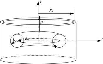
We consider an axisymmetric vortex ring of radius $R_{0}$ placed in an infinitely long rigid tube of radius $R_{w}$ (see figure 1), moving in an incompressible fluid with translational velocity $U$ along the axis of symmetry ( $x$ ). The governing equations for the vorticity ( ${\it\omega}$ ) and streamfunction ( ${\it\Psi}$ ) can be presented as (Batchelor Reference Batchelor1988)

where $x$ , $r$ are the axes of a cylindrical coordinate system and $t$ is time. Note that $\mathscr{L}$ is a linear, self-adjoint elliptic operator. We consider the following boundary conditions: symmetry at the axis,

vanishing vorticity and streamfunction in the far field of the vortex,

and no flow through the tube wall,

Our vortex ring model will be developed using (2.1) and (2.2) with boundary conditions (2.3)–(2.5). Note that boundary condition (2.5) can be used for vortex rings in a tube as long as the viscous interaction of the rings with the tube wall remains weak and can be ignored (see also Brasseur Reference Brasseur1979). For longer time instants, when this assumption is not valid, the boundary condition (2.5) should be replaced with a no-slip wall condition. Note also that DNS in § 3 will use a velocity–pressure formulation of the Navier–Stokes equations, with no-slip boundary conditions at the tube wall.

Figure 1.

Schematic of a vortex ring in a tube.

2.2. Brasseur’s approach to modelling a confined vortex ring

Brasseur (Reference Brasseur1979) modelled a confined vortex ring of circulation ${\it\Gamma}_{0}$ and radius $R_{0}$ (see figure 1) assuming that in the region $r>R_{0}$ the velocity potential ${\it\Phi}_{c}$ is equal to the sum ${\it\Phi}_{c}={\it\Phi}+{\it\Phi}_{0}$ , where ${\it\Phi}$ is the potential of a CVF in an unbounded flow,

and ${\it\Phi}_{0}$ is the velocity potential added to ${\it\Phi}$ to satisfy the boundary condition (2.5) of no flow through the tube wall. The velocity potential ${\it\Phi}$ for a CVF corresponds to the streamfunction (Lamb Reference Lamb1932)

where $\text{J}_{1}$ is the Bessel function of the first kind. Note that formula (2.7) is valid for $x>0$ and the sign of ${\it\Psi}$ is opposite to the one given in Lamb (Reference Lamb1932).

Potential (2.6) can be expanded into a series of harmonic poles at the origin (Brasseur Reference Brasseur1979):

where

The parameter $0<{\it\varepsilon}<1$ quantifies the confinement of the vortex ring. When ${\it\varepsilon}\rightarrow 0$ , the first harmonic can be simplified as

and (2.8) becomes

The first harmonic (2.10) shows that at infinity the vortex ring looks like a point dipole; the contributions of other terms in (2.11) are found as the derivatives with respect to $\tilde{x}$ .

Brasseur (Reference Brasseur1979) replaced the expression of the first harmonic (2.10) with a monopole at the origin in a tube and then derived the velocity potential ${\it\Phi}_{0}$ and the corresponding streamfunction ${\it\Psi}_{0}$ induced by the presence of the tube:

where $\text{K}_{1}$ is the modified Bessel function of the second kind.

Finally, the streamfunction corresponding to a confined vortex ring can be expressed as

where ${\it\Psi}$ is the streamfunction (2.7) of a CVF in an unbounded flow and ${\it\Psi}_{0}$ is the streamfunction (2.13) induced by the presence of the tube.

2.3. A new model for a confined vortex ring

Brasseur (Reference Brasseur1979) modelled a vortex ring as a CVF in a bounded flow. In a new model, described in this section, we apply Brasseur’s approach but replace the vortex filament with the more realistic vortex ring model suggested by Kaplanski & Rudi (Reference Kaplanski and Rudi2005).

We start by recalling the main features of the vortex ring model developed in Kaplanski & Rudi (Reference Kaplanski and Rudi1999, Reference Kaplanski and Rudi2005). Introducing local coordinates (see figure 1)

where $X_{c}$ is the axial coordinate of the vortex centre and $L$ is the diffusivity scale of the ring’s core, the following expressions were obtained: for vorticity,

circulation,

kinetic energy,

translational velocity,

and streamfunction,

where

$\text{J}_{1}$ is the Bessel function of the first kind, $\text{I}_{1}$ is the modified Bessel function of the first kind and $\text{}_{2}\text{F}_{2}$ is the generalised hypergeometric function.

Equations (2.16)–(2.19) were originally derived for $L=\sqrt{2{\it\nu}t}$ , i.e. a laminar vortex ring. Later it was shown that they remain valid in a more general case, when $L$ is approximated as $at^{b}$ , where $a$ and $b$ are constants $(1/4\leqslant b\leqslant 1/2)$ (Kaplanski et al. Reference Kaplanski, Sazhin, Fukumoto, Begg and Heikal2009). This generalised vortex ring model was successfully applied to the analysis of vortex rings observed in petrol internal combustion engines (Begg et al. Reference Begg, Kaplanski, Sazhin, Hindle and Heikal2009; Kaplanski et al. Reference Kaplanski, Sazhin, Begg, Fukumoto and Heikal2010).

At the initial stage when the core is very thin ${\it\nu}t\ll {R_{0}}^{2}({\it\theta}\gg 1)$ , the model describes Saffman’s early-time vortex ring with outer radius $R_{0}$ (Saffman Reference Saffman1970). At this stage the Gaussian form of the vorticity field is strongly compressed and the vorticity isocontours ${\it\omega}/{\it\omega}_{max}$ are circular (Kaplanski, Fukumoto & Rudi Reference Kaplanski, Fukumoto and Rudi2012). At the decaying stage ${\it\nu}t\gg {R_{0}}^{2}({\it\theta}\ll 1)$ , the model predicts the Stokes-dipole solution (Rott & Cantwell Reference Rott and Cantwell1993a ). For these cases, all characteristics of vortex rings, including kinetic energy (2.18) and translational velocity (2.19), at short and long times are given by the closed-form asymptotic expressions and are identical to the well-known Saffman and Rott–Cantwell formulae, respectively. The Gaussian distribution of vorticity predicted by (2.16) at short times agrees with experimental observations of vortex rings (Weigand & Gharib Reference Weigand and Gharib1997; Cater et al. Reference Cater, Soria and Lim2004), although this distribution does not follow from a rigorous solution to the nonlinear Navier–Stokes equation.

To apply the same approach as Brasseur (Reference Brasseur1979), we need to rescale the vortex ring model using the following variables instead of those in (2.15):

In this case the dimensionless vorticity and streamfunction are defined as

We recall that the Reynolds number of the flow was introduced as $\mathit{Re}={\it\Gamma}_{0}/{\it\nu}$ and the parameter ${\it\varepsilon}=R_{0}/R_{w}<1$ quantifies the confinement of the vortex ring. The wall is located at $r_{1w}=1/{\it\varepsilon}$ .

We restrict our analysis to the time interval in which a vortex ring has a well-defined maximum in its vorticity distribution, and is located far from the wall of the tube (small ${\it\varepsilon}$ ). The parameter ${\it\theta}$ (depending on the diffusivity length) is then defined by

Thus, the non-dimensional time can be expressed as

Having substituted (2.22) and (2.24) into (2.16), we obtain the following expression for the non-dimensional vorticity (see Fukumoto & Kaplanski Reference Fukumoto and Kaplanski2008):

The expression for the non-dimensional streamfunction follows from (2.20):

Using the leading term of the expansion for $z_{1}={\it\theta}\sqrt{x_{1}^{2}+r_{1}^{2}}\rightarrow \infty$ , we can obtain an approximation of the streamfunction (2.27) at a large distance from the ring’s core:

Note that the approximation of the streamfunction by (2.28) is valid for positive and negative values of $x_{1}$ and is identical to (2.7). Thus (2.28) describes the streamfunction of a circular filament of vorticity. Therefore, it is expected that the vortex structure, which diffuses with time and transforms into a ‘fat’ vortex ring, has the same large-distance asymptotics as a circular line vortex, identical to Brasseur’s CVF.

Based on this observation, we can find the streamfunction describing the flow generated by a vortex ring in a tube, following the approach suggested by Brasseur (Reference Brasseur1979) (see (2.14)). The dimensionless streamfunction satisfying the boundary conditions (2.3)–(2.5) is presented as

where ${\it\Psi}_{VR}^{\ast }$ is given by (2.27).

Expression (2.29) shows that at large distances, (2.27) transforms into Brasseur’s CVF. Thus at even larger distances this expression will have the same asymptotics as Brasseur’s CVF in the form of the first term of (2.8) (asymptotics for a dipole). Brasseur used this feature and changed asymptotics at large distances to satisfy boundary condition $(1/r)\partial {\it\Psi}/\partial x=0$ at $r=R_{w}$ . 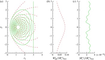As our solution at large distances is identical to Brasseur’s CVF, we expect that the additional streamfunction (2.13) induced by the presence of the tube will act on the combined streamfunction in the same way as described by Brasseur. To illustrate the deformation of the streamlines in the vicinity of the wall, in figure 2 we plot the contours of ${\it\Psi}_{c}^{\ast }$ given by (2.29) and compare them with the streamlines ${\it\Psi}_{VR}^{\ast }$ (given by (2.27)) for the vortex ring in an unbounded domain. Recalling that in the region $r_{1}<1/{\it\varepsilon}$ there are no discontinuities, (2.29) was calculated using the software package Mathematica, Version 6 (Mathematica 2007). It was assumed that ${\it\theta}=3$ and ${\it\varepsilon}=1/3$ . As one can clearly see from figure 2(b,c) displaying streamfunction profiles along the wall boundary ( $r_{1}=r_{1w}=1/{\it\varepsilon}$ ), ${\it\Psi}_{c}^{\ast }$ remains close to zero (and thus satisfies the boundary condition (2.5)) within machine-precision error. ${\it\Psi}_{VR}^{\ast }$ reaches the maximum value at $x_{1}=0$ , which is one order of magnitude below $({\it\Psi}_{c}^{\ast })_{max}$ ; consequently, the wall correction at this point takes its largest value to bring ${\it\Psi}_{c}^{\ast }$ to zero.

Figure 2.

(a) Isocontours of the normalised streamfunctions ${\it\Psi}_{c}^{\ast }/({\it\Psi}_{c}^{\ast })_{max}$ for a confined ring, predicted by (2.29) for ${\it\varepsilon}=1/3,{\it\theta}=3$ (solid curves), and ${\it\Psi}_{VR}^{\ast }/({\it\Psi}_{VR}^{\ast })_{max}$ for an unbounded ring with ${\it\theta}=3$ (see (2.27)) (dashed curves). Contours are shown for ${\it\Psi}_{c}^{\ast }/({\it\Psi}_{c}^{\ast })_{max}$ from 0.1 to 0.9 with an increment of 0.1. The vertical line at $r_{1}=3$ represents the tube wall for the confined ring. Profiles along the tube wall line ( $r_{1}=3$ ) for ${\it\Psi}_{VR}^{\ast }$ (b) and $|{\it\Psi}_{c}^{\ast }|$ (c).

To assess the range of applicability of our model, we estimate below the accuracy of the approximation (2.28) by computing the maximum error at the tube wall. Following figure 2(b,c), the most important correction occurs at $r=R_{w}~(r_{1}=1/{\it\varepsilon})$ for $x_{1}=0$ (corresponding to the vortex centre). This can be theoretically justified by using symmetry considerations (Esteban Reference Esteban1983) and the maximum principle (Fraenkel & Berger Reference Fraenkel and Berger1974). We therefore define the maximum relative error of the model as

where we have used the fact that the maximum value of the streamfunction occurs at the centre of the vortex $(x_{1}=0,r_{1}=1)$ .

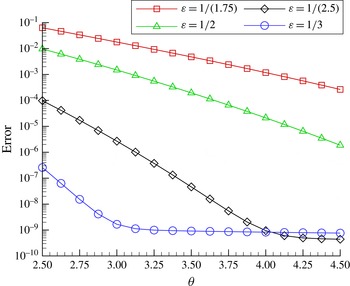
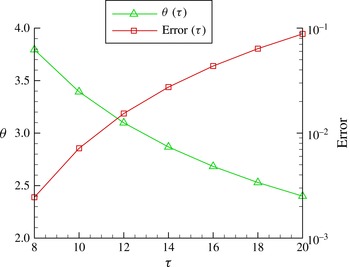
Figure 3 shows the maximum relative error of the model for various confinement parameters ${\it\varepsilon}$ and for a range of the parameter ${\it\theta}$ relative to the values obtained from DNS (see the next sections). We recall that parameter ${\it\theta}$ , defined by (2.24), is a measure of the thickness of the vortex ring (see figure 1). The considered values ( $2.5\leqslant {\it\theta}\leqslant 4.5$ ) correspond to thin vortex rings and are typical of experimentally or numerically generated vortex rings. The maximum error does not exceed 10 % for the strongest confinement ( ${\it\varepsilon}=1/(1.75)$ ) and the thickest vortex ring ( ${\it\theta}=2.5$ ). For ${\it\varepsilon}\geqslant 1/2$ , the errors are negligible for the whole range of parameter ${\it\theta}$ . For typical values most relevant to practical applications (Danaila & Helie Reference Danaila and Helie2008; Fukumoto Reference Fukumoto2010), $3\leqslant {\it\theta}\leqslant 4.5$ , and our confined vortex ring model can be applied with negligible errors for all confinement parameters.

Figure 3.

Maximum relative error of the model defined as the ratio ${\it\Psi}_{c}^{\ast }(x_{1}=0,r_{1}=1/{\it\varepsilon})/({\it\Psi}_{c}^{\ast })_{max}$ , as a function of the parameter ${\it\theta}$ characterising the vortex thickness (see (2.15)). The values of this error were computed for various confinement parameters ${\it\varepsilon}$ using the confined vortex ring model (2.29).

3.1. Numerical model for a vortex ring generator

Laminar vortex rings are usually produced in laboratories by pushing a column of fluid (by a piston/cylinder mechanism, e.g. Gharib, Rambod & Shariff Reference Gharib, Rambod and Shariff1998, or a piston gun, e.g. Sullivan et al. Reference Sullivan, Niemela, Hershberger, Bolster and Donnelly2008) through a long pipe of diameter $D$ . In what follows, all parameters are normalised using $D$ as the length scale and the maximum piston velocity $U_{0}$ as the velocity scale. The main physical parameter of the flow is the Reynolds number based on the pipe diameter:

Using the time scale $t_{0}=D/U_{0}$ , the non-dimensional time in simulations is defined by

where $t^{\ast }$ is the non-dimensional time defined by (2.25) (the same time was used in the theoretical model).

The vortex ring is generated numerically by prescribing an appropriate axial velocity profile at the outlet section of the pipe, corresponding to the inlet section of the computational domain. For this purpose, we used the specified discharge velocity (SDV) model suggested by Danaila et al. (Reference Danaila, Vadean and Danaila2009):

where $U_{p}({\it\tau})$ is the piston velocity program (normalised by its maximum value $U_{0}$ ), $U_{CL}({\it\tau})$ takes into account the time evolution of the centreline velocity, and $U_{b}(r,{\it\tau})$ describes the radial dependence of the profile.

The SDV model is based on the analysis of the Stokes flow evolution inside a long axisymmetric pipe with unitary constant velocity profile at the entry section. At the exit of the pipe, the centreline velocity evolves in time as

The time evolution of the momentum thickness ${\it\Theta}$ and discharge jet radius $R_{jet}$ are given by

where

To describe the radial dependence of the axial velocity profile, the hyperbolic tangent velocity profile (e.g. Michalke Reference Michalke1984) commonly used in jet-flow simulations, was modified to account for the time evolution of its main characteristics:

Note that in most numerical simulations (e.g. James & Madnia Reference James and Madnia1996; Zhao, Steven & Mongeau Reference Zhao, Steven and Mongeau2000), the parameters of the discharge velocity profile are assumed to be constant: $U_{CL}=1$ , $R_{jet}=0.5$ and ${\it\Theta}={\it\Theta}_{0}$ is specified (to prescribe a fixed vorticity layer thickness). This SDV model proved to be very accurate in simulating the laminar vortex ring evolution (see Danaila et al. Reference Danaila, Vadean and Danaila2009), when compared to the available experimental data.

For the piston velocity program we used the model suggested by Zhao et al. (Reference Zhao, Steven and Mongeau2000):

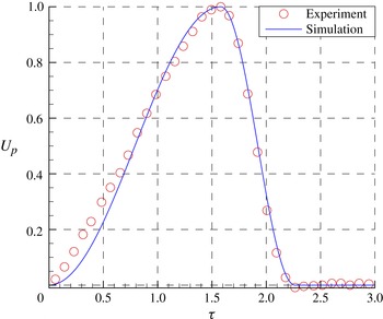
Using the results of recent experiments described by Stewart et al. (Reference Stewart, Niebel, Jung and Vlachos2012), the following fitting constants were obtained (see figure 4): ${\it\tau}_{1}=1.57$ and ${\it\tau}_{2}=2.26$ .

Figure 4.

Piston velocity $U_{p}({\it\tau})$ used for numerical simulations (solid curve) and experimentally observed piston velocity reported by Stewart et al. (Reference Stewart, Niebel, Jung and Vlachos2012) (symbols).

The main integral characteristics of the vortex generator can be approximately estimated by the so-called slug model (Shariff & Leonard Reference Shariff and Leonard1992; Lim & Nickels Reference Lim, Nickels and Green1995). This model assumes that at the exit plane of the vortex generator the flow is parallel to the axis and the rate of change of the circulation is determined by the vorticity flux across this plane. Thus, the stroke length ( $L_{p}$ ), circulation ( ${\it\Gamma}_{p}$ ), impulse ( $I_{p}$ ) and kinetic energy ( $E_{p}$ ) of the discharged fluid at the cylinder tip are calculated as

Taking $\mathit{Re}_{D}=1770$ and ${\it\tau}_{off}=2.26$ , as in the experiments by Stewart et al. (Reference Stewart, Niebel, Jung and Vlachos2012), we obtain from (3.4) and (3.10) the following values: $L_{p}=1.28$ , ${\it\Gamma}_{p}=0.55$ , $I_{p}=0.86$ , $E_{p}=0.41$ .

Note that the stroke ratio ( $L_{p}=1.28$ ) is lower than the so-called formation number of the vortex ring, reported to be in the range 3.6–4.5 (Gharib et al. Reference Gharib, Rambod and Shariff1998; Krueger & Gharib Reference Krueger and Gharib2003; Dabiri & Gharib Reference Dabiri and Gharib2005). This implies that all the vorticity produced by the vortex generator is expected to be engulfed by the vortex ring, i.e. the separation (pinch-off) between the vortex ring and its tail, observed for stroke ratios exceeding 4, is not expected to be present for this case.

3.2. Numerical results

We use the same computational setting as in Danaila & Helie (Reference Danaila and Helie2008) and in Danaila et al. (Reference Danaila, Vadean and Danaila2009), since the long time evolution of a laminar vortex ring was accurately captured in these studies. The length of the computational domain was taken as $L_{d}=10$ , which allowed us to avoid the vortex ring coming close to the downstream boundary, where we apply the convective boundary condition (Orlanski Reference Orlanski1976), enforced by the global mass conservation procedure suggested by Ruith et al. (Reference Ruith, Chen and Meiburg2004). At $r=R_{w}$ a no-slip boundary condition is imposed through a ghost-cell procedure. The grid was uniform in both the axial and radial directions with a refined grid size ${\it\delta}r={\it\delta}x=0.01$ , which ensures grid convergence of the results. Tests with a stretched grid in the radial direction, such that at least 30 grid points are clustered in the vorticity layer at the inflow, showed identical results. The timestep was set to ${\it\delta}{\it\tau}=0.001$ , which is largely below the admissible value imposed by the stability of the numerical scheme. Timestep refinement tests showed negligible differences in the results obtained for lower ${\it\delta}{\it\tau}$ .

To investigate the physics of a confined vortex ring, we first fix the confinement parameter and assume that $D_{w}/D=1.75$ , as inferred from the experiments by Stewart et al. (Reference Stewart, Niebel, Jung and Vlachos2012). Note that this confinement parameter is more appropriate for describing experiments or numerical simulations than the parameter ${\it\varepsilon}=D_{0}/D_{w}$ defined in the theoretical analysis. Indeed, the value of the diameter of the vortex ring $D_{0}$ (see figure 1) cannot be specified after prescribing the injection parameters. The two parameters are related by the formula $D_{w}/D=D_{0}/({\it\varepsilon}D)$ ; a very rough approximation of the latter relation leads to the following expression: $D_{w}/D\approx 1/{\it\varepsilon}$ .

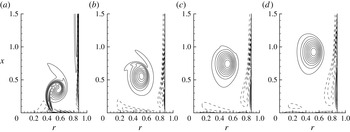
The early stages of the vortex ring formation are illustrated by contours of vorticity in figure 5. Due to a very small piston stroke ratio, a vortex forms rapidly near the inlet section. The vortex ring evolves near the lateral wall, generating a negative vorticity layer that interacts with the stopping vortex, which is produced at the inlet section after the injection stops ( ${\it\tau}>{\it\tau}_{off}=2.26$ ). Note that we did not model the termination of the injection process, since our analysis referred to the cases when injections stopped suddenly. The stopping vortex normally travels back into the vortex generator and does not interact with the vortex ring (see the discussion by Krueger Reference Krueger2008).

Figure 5.

Contours of vorticity ${\it\omega}$ at the early stage of formation of the vortex ring in a tube. Dashed curves show contours of negative vorticity. Times: (a)  ${\it\tau}=2$ , (b)  ${\it\tau}=3$ , (c)  ${\it\tau}=4$ , (d)  ${\it\tau}=5$ ; $\mathit{Re}_{D}=1700$ , $D_{w}/D=1.75$ .

Figure 6.

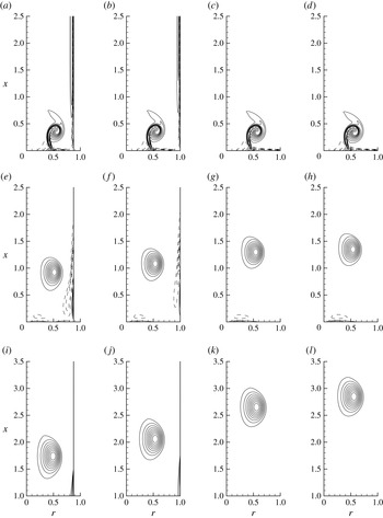
Contours of the normalised vorticity ${\it\omega}/{\it\omega}_{max}$ at various time instants and confinement parameters. Times: (a–d) ${\it\tau}=2$ , (e–h) ${\it\tau}=5$ , (i–l) ${\it\tau}=10$ . Parameters: (a,e,i) $D_{w}/D=1.75$ , (b,f,j) $D_{w}/D=2$ , (c,g,k) $D_{w}/D=3$ , (d,h,l) $D_{w}/D=8$ ; $\mathit{Re}_{D}=1700$ . The values of vorticity increase from $-0.3$ to 0.9 with increments of 0.1; dashed curves show contours of negative vorticity.

The influence of the confinement parameter $D_{w}/D$ on the vortex ring evolution is illustrated in figure 6. During the injection phase ( ${\it\tau}\leqslant {\it\tau}_{off}=2.26$ ) the formation of the vortex ring is not affected by the proximity of the wall. This was also observed in the experimental study by Stewart et al. (Reference Stewart, Niebel, Jung and Vlachos2012). After the injection stops, the vortex ring moves faster when $D_{w}/D$ increases, i.e. the confinement is reduced (see figure 6 for ${\it\tau}=5$ and ${\it\tau}=10$ ). This is attributed to the interaction of the vortex ring with the vorticity layer (of the opposite sign) induced at the wall (the details of the wall vorticity are visible in figure 5 for ${\it\tau}=5$ ). Also, one can observe from figure 6 that the influence of confinement becomes negligible for large $D_{w}/D$ . 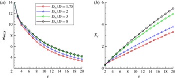Our simulations showed that for $D_{w}/D\geqslant 3$ , the lateral wall does not produce a significant impact on the vortex ring evolution. This observation is also supported by the analysis of the time evolution of the parameters characterising the vortex ring strength and trajectory: the maximum value of the vorticity ${\it\omega}_{max}$ (figure 7 a) and the streamwise position $X_{c}$ (figure 7 b) of the vortex centre corresponding to the maximum vorticity. As expected, the value of ${\it\omega}_{max}$ for the vortex ring becomes larger and the ring travels faster when the confinement is reduced ( $D_{w}/D$ is increased). For $D_{w}/D\geqslant 3$ the results are very close to the case $D_{w}/D=8$ , which can represent the asymptotic regime of an unconfined vortex ring. We can conclude that the influence of the lateral wall is negligible for $D_{w}/D\geqslant 3$ , which is consistent with previously reported experimental findings (Stewart et al. Reference Stewart, Niebel, Jung and Vlachos2012).

Figure 7.

Time evolution of maximum vorticity ${\it\omega}_{max}$ and streamwise position of the vorticity centre $X_{c}$ corresponding to the maximum vorticity; $\mathit{Re}_{D}=1700$ .

Figure 8.

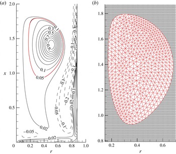
(a) Contours of the normalised vorticity ${\it\omega}/{\it\omega}_{max}$ for the vortex ring at ${\it\tau}=8$ ; $\mathit{Re}_{D}=1700,D_{w}/D=1.75$ . Dashed curves show contours of negative vorticity. (b) Illustration of the post-processing procedure using finite elements: the contour ${\it\omega}/{\it\omega}_{max}=0.05$ is identified and then the inside area is remeshed using triangular finite elements (this close-up of the finite element mesh using larger triangles is shown for clarity).

The main finding by Stewart et al. (Reference Stewart, Niebel, Jung and Vlachos2012) was that the circulation of the vortex ring during the post-formation phase rapidly decreases in the presence of the lateral wall. To compute vortex ring circulation, the vortex core must be properly separated from the background flow. Usually the centre $C$ of the vortex is first located as the point of the maximum vorticity ${\it\omega}_{max}$ ; the vortex core is then defined as the inner domain bounded by the vorticity contour ${\it\omega}/{\it\omega}_{max}=0.05$ that encircles the centre $C$ . The cutoff level is set based on trial and error, to the best satisfaction of the authors. Threshold values ranged from 2 % (Mohseni Reference Mohseni2001) and 5 % (Rosenfeld, Rambod & Gharib Reference Rosenfeld, Rambod and Gharib1998; Zhao et al. Reference Zhao, Steven and Mongeau2000; Sau & Mahesh Reference Sau and Mahesh2007) in numerical studies, to approximately 10 % (Dabiri & Gharib Reference Dabiri and Gharib2004) in experiments.

The presence of the lateral wall makes the separation of the vortex core rather delicate, since intense vorticity layers develop near this wall and at the inflow section after the injection stops. A special post-processing program, based on the free finite element solver FreeFem $++$ (Hecht et al. Reference Hecht, Pironneau, Hyaric and Ohtsuke2007; Hecht Reference Hecht2012), was designed to properly separate the vortex ring core and compute flow integrals. The program identifies all closed contours for the prescribed threshold of ${\it\omega}/{\it\omega}_{max}$ (see figure 8), selects the unique contour around the vortex ring centre and then meshes this domain with triangles. All flow characteristics are then represented on the finite element mesh using quadratic $P_{2}$ triangular elements. The interpolation between the finite difference grid (used for DNS computations) and the finite element mesh is also quadratic, which is consistent with the spatial accuracy of the Navier–Stokes solver. The advantage of this finite element post-processing is that it enables us to represent accurately and smoothly the boundary of the vortex core and, then, to use high-order (up to seventh-order) Gaussian methods to compute the integral characteristics (circulation, impulse, energy) presented in the following section. Also, this post-processing toolbox can be easily used to post-process experimental results (obtained from PIV measurements), since FreeFem $++$ is an integrated product with its own high-level programming language with a syntax close to mathematical formulations.

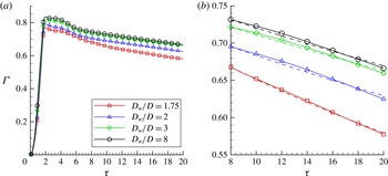
The time evolution of circulation corresponding to vortex ring cores separated using this method is shown in figure 9(a). After rapid increase during the injection phase ( ${\it\tau}\leqslant {\it\tau}_{off}=2.26$ ), the circulation attains a small plateau ( $2.26\leqslant {\it\tau}\leqslant 6$ ) and then starts to decrease in the post-formation phase. Assuming that the vortex ring is completely formed when the contour line ${\it\omega}/{\it\omega}_{max}=0.05$ defines a convex set (see figure 8), the post-formation phase starts at ${\it\tau}=8$ . A close-up of the time evolution of circulation during this phase is shown in figure 9(b). A higher rate of decrease of the circulation is observed when the confinement is increased (the ratio $D_{w}/D$ is decreased). This is consistent with experimental observations by Stewart et al. (Reference Stewart, Niebel, Jung and Vlachos2012), who suggested that the time evolution of the circulation ${\it\Gamma}({\it\tau})$ can be described by the ordinary differential equation $\text{d}{\it\Gamma}/\text{d}{\it\tau}=-{\it\beta}{\it\Gamma}^{2}$ with the solution

where ${\it\Gamma}_{f}$ refers to the (fitted) circulation at ${\it\tau}={\it\tau}_{f}$ ( ${\it\Gamma}_{f}$ was taken as the peak circulation in the experiments). The predictions of (3.11), taking ${\it\tau}_{f}=8$ , and shown in figure 9(b) are in good agreement with DNS results. The fitting coefficient ${\it\beta}$ , which is related to the production of vorticity at the confinement wall, decreases with increasing $D_{w}/D$ , although not exponentially, as reported by Stewart et al. (Reference Stewart, Niebel, Jung and Vlachos2012). This could be related to the fact that our fit refers to a long time evolution during the post-formation phase, while Stewart et al. (Reference Stewart, Niebel, Jung and Vlachos2012) considered a very short time interval after the injection stopped. We can conclude that the model equation (3.11) can be used to describe the decrease in circulation even during the post-formation phase.

Figure 9.

(a) Time evolution of the vortex ring circulation for four values of the confinement parameter $D_{w}/D$ . (b) Close-up corresponding to the post-formation phase of the vortex ring evolution. Dashed curves show the results inferred from (3.11) suggested by Stewart et al. (Reference Stewart, Niebel, Jung and Vlachos2012).  $\mathit{Re}_{D}=1700$ .

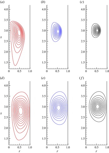
The influence of the viscous diffusion on the flow physics was investigated by performing the simulations for three Reynolds numbers. Figure 10 shows the vorticity and streamfunction distributions for the time instant ${\it\tau}=15$ , confinement parameter $D_{w}/D=2$ and 3 values of $\mathit{Re}_{D}$ . For $\mathit{Re}_{D}=500$ , the vortex ring diffuses rapidly and generates large regions of opposite vorticity at the confinement wall; the post-formation phase is not clearly defined in this case, since the vortex ring almost fills the tube. For larger Reynolds numbers ( $\mathit{Re}_{D}=3400$ ), the vorticity distribution looks more compact than for $\mathit{Re}_{D}=1700$ , used in previous plots and in experiments by Stewart et al. (Reference Stewart, Niebel, Jung and Vlachos2012). This suggests that to test our analytical model using DNS data we need to use not only the reference value $\mathit{Re}_{D}=1700$ , but also the more challenging case of higher Reynolds number $\mathit{Re}_{D}=3400$ .

Figure 10.

Contours of (a–c) normalised vorticity ${\it\omega}/{\it\omega}_{max}$ and (d–f) the corresponding normalised streamfunction ${\it\psi}/{\it\psi}_{max}$ , for the time instant ${\it\tau}=15$ and confinement parameter $D_{w}/D=2$ ; (a,d)  $\mathit{Re}_{D}=500$ , (b,e)  $\mathit{Re}_{D}=1700$ , (c,f)  $\mathit{Re}_{D}=3400$ . The values of ${\it\omega}/{\it\omega}_{max}$ and ${\it\psi}/{\it\psi}_{max}$ are shown from 0.1 to 0.9 with increments of 0.1.

4.1. Comparison algorithm

To enable us to compare the predictions of the model and DNS results, we assume that the pinch-off (Gharib et al. Reference Gharib, Rambod and Shariff1998; Mohseni Reference Mohseni2001), i.e. the separation between the vortex ring and the vorticity tail, has taken place and the vortex ring is completely formed. Thus, we consider the vortex ring evolution over large time intervals during the post-formation phase.

The comparison of the predictions of the model with DNS data starts with fitting the vortex rings, obtained by DNS and the model at a given time instant ${\it\tau}={\it\tau}_{f}$ . We use (2.16) for the vorticity distribution, with the approximation $\text{I}_{1}({\it\sigma}{\it\theta})\approx \exp ({\it\sigma}{\it\theta})/\sqrt{2{\rm\pi}{\it\sigma}{\it\theta}}$ , valid for large ${\it\theta}$ . For the cases shown below ${\it\theta}>4$ , which makes this approximation possible. Thus, we fit the DNS vorticity field with the expression

Parameters ${\it\Gamma}_{f},R_{0f},X_{cf},L_{f}$ are found using a nonlinear fit (BFGS minimisation method) integrated in the finite-element post-processing algorithm. We compute ${\it\theta}_{f}=R_{0f}/L_{f}$ to complete the definition of the corresponding theoretical vortex ring. Formula (2.16) is then used to reconstruct the theoretical vorticity field ${\it\omega}(r,x)$ and compute integral characteristics in the same way as in DNS (taking into account only the vorticity of the vortex core for which ${\it\omega}/{\it\omega}_{max}>0.05$ ).

After fitting the DNS vortex with the prediction of the model at ${\it\tau}={\it\tau}_{f}$ , we can predict the time evolution of integral characteristics assuming (see (2.25)) that

The non-dimensional circulation ( ${\it\Gamma}^{\ast }$ ), energy ( $E^{\ast }$ ) and translational velocity ( $U^{\ast }$ ) predicted by the model are then calculated using ${\it\omega}^{\ast }$ given by (2.26) and ${\it\Psi}_{c}^{\ast }$ by (2.29):

The links between non-dimensional characteristics used for the model (starred variables) and corresponding characteristics used in DNS computations (we recall that $t_{DNS}={\it\tau}$ ) are given by the following expressions:

In what follows, all the characteristics are referred to using DNS (non-starred) variables.

Finally, the translational velocity of the vortex ring is computed from DNS data as

where $X_{{\it\omega}c}$ is the streamwise coordinate of the vorticity centroid (Hill Reference Hill1894; Krieg & Mohseni Reference Krieg and Mohseni2013). This will be compared to that given by (4.5).

Figure 11.

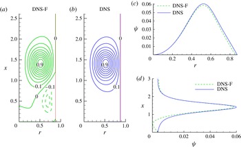
Contours of normalised streamfunction ${\it\psi}/{\it\psi}_{max}$ obtained by solving (2.2) numerically with the right-hand side term corresponding to the full DNS vorticity field (a, DNS-F) and to the vorticity inside the vortex ring core ( ${\it\omega}/{\it\omega}_{max}\geqslant 0.05$ ) (b, DNS). Streamfunction profiles through the centre of the vortex: (c) along the $r$ -axis ( $x=X_{c}$ ), (d) along the $x$ -axis ( $r=R_{0}$ ).  $\mathit{Re}_{D}=1700$ , $D_{w}/D=1.75$ , ${\it\tau}=8$ .

Figure 12.

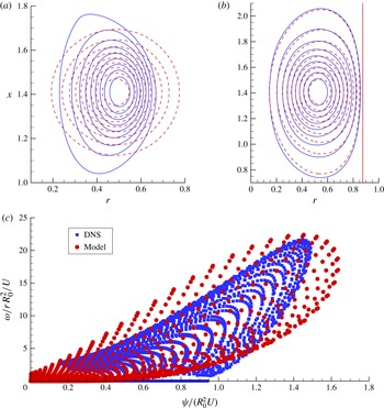
Comparison between the DNS data (blue solid curves or squares) and predictions of the vortex ring model (red dashed curves or circles). (a) Contours of normalised vorticity ${\it\omega}/{\it\omega}_{max}$ ; (b) corresponding contours of normalised streamfunction ${\it\psi}/{\it\psi}_{max}$ ; (c) scatter plot $\{{\it\psi}_{p},{\it\omega}_{p}/r_{p}\}$ (non-dimensional values) for points $p$ inside the vortex ring core. Values of ${\it\omega}/{\it\omega}_{max}$ and ${\it\psi}/{\it\psi}_{max}$ from 0.1 to 0.9 with increments of 0.1 are shown in (a) and (b). $\mathit{Re}_{D}=1700$ , $D_{w}/D=1.75$ , ${\it\tau}=8$ .

4.2. Streamfunction field of the confined vortex ring for $\mathit{Re}_{D}=1700$

First we consider the case $\mathit{Re}_{D}=1700$ , $D_{w}/D=1.75$ studied in the previous section and used in the experiments described by Stewart et al. (Reference Stewart, Niebel, Jung and Vlachos2012). We focus on the post-formation phase ( ${\it\tau}\geqslant 8$ ) characterised by a decay in circulation with time (see figure 9). We recall that for DNS data, streamfunction ${\it\psi}$ is computed by solving numerically (2.2) with the vorticity corresponding to the vortex ring core ( ${\it\omega}/{\it\omega}_{max}\geqslant 0.05$ ). The vorticity layer generated at the wall is thus ignored, to allow comparison with the theoretical model which does not take into account such effects. From figure 8 it can be seen that the negative vorticity at the lateral wall is rather small ( $|{\it\omega}/{\it\omega}_{max}|\leqslant 0.01$ ). Its influence on the spatial distribution of the streamfunction is thus expected to be limited to the downstream part of the vortex ring. Figure 11 illustrates this statement by displaying streamfunction fields calculated using the full vorticity field (DNS-F, figure 11 a) and the vorticity of the vortex ring core only (DNS, figure 11 b). Streamfunction profiles through the centre of the vortex, along the $r$ -axis (figure 11 c) and $x$ -axis (figure 11 d) show that differences between the two cases are negligible inside the vortex ring core. Therefore, we will use DNS streamfunction fields corresponding to the vorticity truncated to zero outside the vortex ring core.

In figure 12 the results of comparison of the DNS data with the predictions of the vortex ring model for ${\it\tau}=8$ are shown. As expected, the vortex ring model (see (2.16) and its approximation (4.1) with an isotropic two-dimensional Gaussian) predicts quasi-circular contours for vorticity, compared to the prolate shape contours for the DNS vortex. 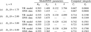Nevertheless, the nonlinear fit provides accurate localisation of the vortex centre $(R_{0f},X_{cf})$ , as indicated in table 1(a). Also, the circulation predicted by the vortex ring model is very close to that obtained for the DNS vortex. Note that the model for a confined vortex ring is based on the assumption that the space distribution of the vorticity is not very important in deriving (2.29) for the streamfunction. This is confirmed by the results shown in figure 12(b) demonstrating very good agreement between DNS data and predictions of the model for the normalised streamfunction contours. Streamlines predicted by the model are almost circular close to the vortex centre, but deform near the wall to accommodate the wall boundary condition, as in the case of DNS results. The lateral wall located at $R_{w}=0.875$ is captured as a streamline in both cases.

Table 1.

Parameters of the vortex ring model obtained by a nonlinear fit of (4.1) using DNS data and that computed from the original DNS for various confinement ratios $D_{w}/D$ . The results of comparison are presented for the vortex centre position ( $R_{0f},X_{cf}$ ), circulation ${\it\Gamma}_{f}$ and energy $E_{f}$ .  $\mathit{Re}_{D}=1700$ , ${\it\tau}_{f}=8$ .

Figure 12(a,b) also suggests that the DNS vortex ring could not be accurately described by models derived as steady solutions to Euler equations (e.g. the Norbury model). For inviscid and steady flows, the vorticity equation (2.1) reduces to ${\it\omega}/r=F({\it\Psi})$ , with $F$ being an arbitrary function, i.e. ${\it\omega}/r$ propagates without change of shape along streamlines. For such models, a good theoretical representation of the streamfunction field would also guarantee an accurate representation of the vorticity field, which is not the case in figure 12(a,b). In order to explore this feature, we present in figure 12(c) a scatter plot of ${\it\omega}/r$ as a function of ${\it\Psi}$ for points inside the vortex ring core. We have plotted normalised values of vorticity and streamfunction, as in Sullivan (Reference Sullivan1973), using the vortex ring radius $R_{0}$ and the translation velocity $U$ as reference scales. As one can see from this figure, ${\it\omega}/r$ cannot be represented as a simple function of ${\it\psi}$ , either for the model, or for the DNS vortex. Similar scatter plots were reported in experimental studies of unconfined vortex rings (Sullivan Reference Sullivan1973; Akhmetov Reference Akhmetov2009). The fact that our model is based on the Kaplanski–Rudi model, including viscous and unsteady effects (see § 2.3 and (2.24)), allows us to obtain a scatter plot which is very close to that obtained by DNS.

Figure 13.

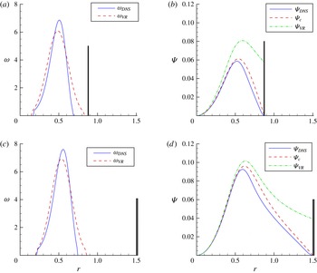
Comparison between the DNS data (blue solid curves) and predictions of the vortex ring model (red dashed curves). Profiles are shown along the $r$ -axis through the centre of the vortex (at $x=X_{c}$ ). Vorticity ${\it\omega}$ and streamfunction ${\it\psi}$ profiles are shown for two confinements $D_{w}/D=1.75$ (a,b) and $D_{w}/D=3$ (c,d). Streamfunction profiles ( ${\it\Psi}_{VR}$ ) of the unconfined vortex ring (2.20) are shown (green dash-dot curves) for reference in figures (b) and (d). Vertical lines indicate the lateral wall. $\mathit{Re}_{D}=1700$ , ${\it\tau}=8$ .

Figure 14.

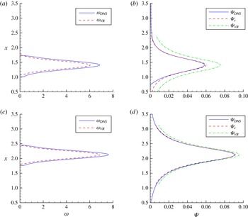
The same as in figure 13, but for the profiles along the $x$ -axis through the centre of the vortex (at $r=R_{0}$ ).  $D_{w}/D=1.75$ (a,b) and $D_{w}/D=3$ (c,d).

To explore the accuracy of our model, we showed in figures 13 and 14 vorticity and streamline profiles through the centre of the vortex. Profiles along the $r$ -axis are the most representative, since the presence of the wall at $r=R_{w}$ must be taken into account. Two confinement ratios are considered: $D_{w}/D=1.75$ and $D_{w}/D=3$ . Vorticity profiles (figure 13 a,c) are well approximated by the model, even though the theoretical vorticity (see (2.16) and its approximation (4.1) by an isotropic two-dimensional Gaussian) does not reproduce the asymmetry of the DNS vorticity profile with respect to the centre of the vortex. We recall that the Gaussian approximation (4.1) stands for relatively thin vortex rings, with small diffusive scales $L$ . The asymmetry of vorticity profiles is less important along the longitudinal $x$ -axis (figure 14 a,c), making the theoretical predictions very accurate. In figure 13(b,d), in addition to the streamline profile ( ${\it\Psi}_{c}$ ) of the confined vortex ring (see (2.29)) we also plot the streamline profile ( ${\it\Psi}_{VR}$ ) of the unconfined vortex ring (see (2.27)). It can be clearly seen from these figures that the correction ${\it\Psi}_{0}$ added in (2.29) plays an important role in bringing ${\it\Psi}_{c}$ to zero at the wall. We recall that $\mathscr{L}{\it\Psi}_{0}=0$ and thus it does not affect the vorticity distribution of the vortex ring. The correction is most visible in the vicinity of the wall ( $R_{0}<r<R_{w}$ ) and allows us to obtain a very good approximation of the DNS profiles. We also note that, as expected, the correction is most important for the low confinement ratio ( $D_{w}/D$ ) since in this case the wall is at its closest to the vortex centre. In the longitudinal $x$ -direction (figure 14 b,d), the correction due to the wall is less important since the unconfined vortex ring model already gives a good approximation ( ${\it\Psi}_{VR}\approx {\it\Psi}_{c}$ ).

Note that the quasi-superposition of streamlines implies that the DNS and theoretical vortex rings have similar signatures. The signature of a vortex ring without swirl is a topological invariant, defined by Moffatt (Reference Moffatt1988) as the volume inside the torus ${\it\psi}=\text{const.}$ (see also Danaila & Helie Reference Danaila and Helie2008).

Table 1 shows the comparison between the predictions of DNS and modelling for three other confinement parameters $D_{w}/D=2,3,8$ . For small confinements (large $D_{w}/D$ ) the model tends to overestimate the circulation of the vortex ring, but by no more than 3 %. The values of the energy $E_{f}$ , computed from (4.4) using the fitted vorticity distribution, are in very good agreement with the DNS results for all confinement ratios. This implies that the theoretical model for the streamfunction ${\it\Psi}_{c}$ is not only qualitatively accurate (as shown in figure 12), but can also be used for quantitative characteristics of vortex rings.

4.3. Evolution of integral characteristics for $\mathit{Re}_{D}=1700$

In the next step, the time evolutions of integral characteristics (circulation, energy and translational velocity), predicted by the model with viscous length given by (4.2), are compared with those obtained by DNS. The vorticity field was truncated so that only values ${\it\omega}/{\it\omega}_{max}\geqslant 0.05$ , representing the vortex core, were considered. Using the fitted vortex ring at ${\it\tau}=8$ (with parameters displayed in table 1) we computed model predictions corresponding to the time evolution of the viscous scale given by (2.24) for a long time interval $8\leqslant {\it\tau}\leqslant 20$ . To check whether this case lies inside the range of applicability of the model (see § 2.3 and figure 3), we plotted in figure 15 the time evolution of parameter ${\it\theta}$ and the corresponding maximum relative errors of the model (see (2.30)). As follows from figure 15, the model offers a very good approximation, despite the strong confinement (corresponding to ${\it\varepsilon}\approx 1/(1.75)$ in figure 3).

Figure 15.

Time evolution of parameter ${\it\theta}$ assumed in the model (see (2.24)) and corresponding maximum relative error intrinsic to the model (see (2.30)).  $\mathit{Re}_{D}=1700$ .

Figure 16.

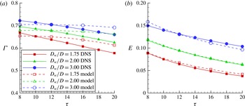
Time evolution of the circulation ${\it\Gamma}$ (a) and energy $E$ (b) of the vortex ring obtained by DNS and the model for three confinement parameters $D_{w}/D$ .  $\mathit{Re}_{D}=1700$ .

Figure 17.

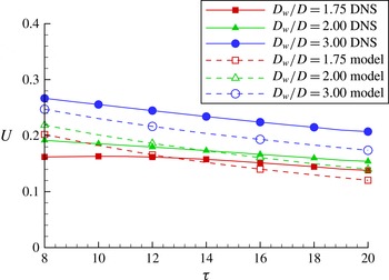
Time evolution of the translational velocity $U$ of the vortex ring. Comparison between DNS data and the model predictions (4.5) for three confinement parameters $D_{w}/D$ .  $\mathit{Re}_{D}=1700$ .

The time evolution of circulation and energy, predicted by the model and DNS for confinement parameters $D_{w}/D=1.75$ , 2 and 3, are shown in figure 16. For the sake of clarity, the plots for $D_{w}/D=8$ , which were very close to the plots for the case $D_{w}/D=3$ , are not shown in the figure. Remembering equation (2.17), one can expect that the circulation predicted by the model is close to ${\it\Gamma}_{f}$ considered at the fitting time ${\it\tau}={\it\tau}_{f}$ . Figure 16(a) shows that the rate of decrease of circulation inferred from DNS data is higher than the one predicted by the model. However, theoretical values of ${\it\Gamma}$ are very close to DNS values, especially if smaller time intervals are considered. This explains why the time evolutions of energies, inferred from DNS data and predicted by the model (see figure 16 b), are close. The idea behind this comparison was to challenge our model to predict the time evolution of integral characteristics for long time intervals. Strictly speaking, this is beyond the capabilities of the model, since the original Kaplanski–Rudi vortex ring model is valid for small time intervals when the Reynolds number is large (Fukumoto & Kaplanski Reference Fukumoto and Kaplanski2008). However, figure 16 shows that the model could also be applied for large time evolutions, with fairly good accuracy. This opens the way to using the model for realistic configurations of practical interest.

Finally, we compare the theoretical prediction (4.5) for the translational velocity of the vortex ring with the DNS values computed from the time evolution of the vorticity centroid (4.8) (see figure 17). We recover two of the characteristic features of the vortex ring motion discussed in § 2: the translational velocity $U$ is larger for low confinements (large $D_{w}/D$ ratios) and $U$ decreases faster when the confinement is low. These are two consequences of the interaction of the vortex ring with the vorticity created near the lateral wall (with the sign opposite to the vorticity of the vortex ring). Our model accounts for these features of the confined vortex ring motion, but the values of $U$ are underestimated compared to those obtained by DNS. The origin of these discrepancies is the role of the streamwise gradient $\partial {\it\Psi}_{c}^{\ast }/\partial x_{1}$ present in (4.5); theoretical streamfunction ${\it\Psi}_{c}^{\ast }$ displays larger gradients near the wall than those inferred from the DNS field, resulting in lower values of the translational velocity predicted by the model. The model, however, is able to predict well the main features of the variation of the translational velocity of the confined vortex ring.

4.4. Evolution of integral characteristics for higher Reynolds numbers

In an attempt to further challenge our model, we considered the case of a higher Reynolds number ( $\mathit{Re}_{D}=3400$ ) and long time evolution of the vortex ring during the post-formation phase. We kept the same injection program (see figure 4) with ${\it\tau}_{off}=2.26$ and focused on $15\leqslant {\it\tau}\leqslant 60$ . DNS computations were performed on a larger domain ( $L_{d}=20$ ) to account for the long time evolution. We used the same spatial resolution and the same timestep as for previous simulations to ensure mesh convergence of the results. Confinement parameters $D_{w}/D\geqslant 2$ were considered in order to avoid the situation where the vortex ring touches the lateral wall during long time evolutions. Figure 18 shows a comparison between the values of normalised vorticity and streamfunction predicted by the model and DNS at ${\it\tau}=15$ and $D_{w}/D=2$ . 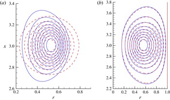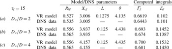As one can see in this figure, the time evolution trends for both parameters, predicted by the model and obtained by DNS, are rather similar. This means that the two vortex rings have the same signature, despite rather different spatial distributions of the vorticity. Table 2 summarises the predictions of the main parameters defining the vortex rings for various confinement parameters $D_{w}/D$ . 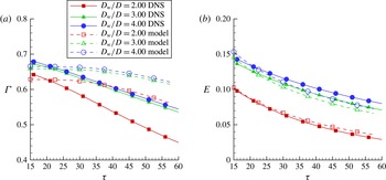The spatial positions of the vortex are accurately captured by the model, whilst it slightly overestimates the initial circulation. The time evolutions of the vortex ring circulation and energy are compared in figure 19. We notice in this figure the same trends as for $\mathit{Re}_{D}=1700$ : the theoretical rate of circulation decay is lower than inferred from DNS data, while the energy predictions made by the model are very close to numerical results.

Figure 18.

Contours of normalised vorticity ${\it\omega}/{\it\omega}_{max}$ (a) and corresponding normalised streamfunction ${\it\psi}/{\it\psi}_{max}$ (b), obtained by DNS (blue solid curves) and the vortex ring model (red dashed curves). The values of ${\it\omega}/{\it\omega}_{max}$ and ${\it\psi}/{\it\psi}_{max}$ are shown from 0.1 to 0.9 with increments of 0.1. $\mathit{Re}_{D}=3400$ , $D_{w}/D=2$ , ${\it\tau}=15$ .

Figure 19.

Time evolution of the circulation ${\it\Gamma}$ (a) and energy $E$ (b) of the vortex ring, as inferred from DNS data and predicted by the model for three confinement parameters $D_{w}/D$ .  $\mathit{Re}_{D}=3400$ .

Table 2.

Parameters of the vortex ring model obtained by a nonlinear fit of (4.1) using DNS data and that computed from the original DNS for various confinement ratios $D_{w}/D$ . The results of comparison are presented for the vortex centre position ( $R_{0f},X_{cf}$ ), circulation ${\it\Gamma}_{f}$ and energy $E_{f}$ .  $\mathit{Re}_{D}=3400$ , ${\it\tau}_{f}=15$ .