


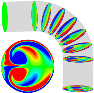



1. Introduction
Unsteady flows along circular pipes are among the most studied fluid mechanics problems, encompassing a type of geometry (the circular tube) and a type of flow driven by a heart (Rindt et al. Reference Rindt, Van Steenhoven, Janssen and Vossers1991; Najjari & Plesniak Reference Najjari and Plesniak2016) or a pump (Singh & Madavan Reference Singh and Madavan1987; Miller Reference Miller1987, Reference Miller1988; Vetter & Schweinfurther Reference Vetter and Schweinfurther1987; Manring Reference Manring2000) common in nature and industry, respectively. Unsteady pipe flows in this context are broadly distinguished based on whether the flow at some stage reverses (Sudo, Sumida & Yamane Reference Sudo, Sumida and Yamane1992) or remains positive (Singh & Madavan Reference Singh and Madavan1987; Miller Reference Miller1987, Reference Miller1988; Vetter & Schweinfurther Reference Vetter and Schweinfurther1987; Sumida, Sudou & Wada Reference Sumida, Sudou and Wada1989; Takeshi et al. Reference Takeshi, Yoshihiro, Sachiko and Kazuo1990; Komai & Tanishita Reference Komai and Tanishita1997; Manring Reference Manring2000; Krishna, Gundiah & Arakeri Reference Krishna, Gundiah and Arakeri2017). The combination of flow unsteadiness and piping geometrical discontinuity (curved pipes) leads to large unsteady forces, which is problematic with respect to the piping stress and vibration. In the energy sector (oil and gas industry), the consequence of excessive pipeline stresses and vibration is the loss in structural integrity (for example, fatigue failures, instrument distortion and process efficiency) and production downtime.
The purpose of this paper is to understand the influence of a pulsatile flow on pipe bend force and secondary flow when the Strouhal number ( $St$) is high and flow acceleration is important. This is illustrated with an example where the volume flux is
 $Q=U_b A |\sin \varOmega _p t|$, which is typical of the idealised flow generated by high-energy reciprocating pumps. This type of pulsatile flow has a root-mean-square (r.m.s.) comparable to the mean, and is characterised by a discontinuity in the flow acceleration, so both the mean (steady) and oscillatory components are essential for the secondary flow. The general analysis developed will be relevant to a broader range of high-
 $St$ inertially dominated pulsatile flows irrespective of the nature of volume flux.
We discuss the main contributions to the secondary flow analysis first. The motivation for examining steady flows in curved pipes has been driven mainly by observing a weak secondary flow that remains persistent after a pipe bend. The commonly observed meandering of rivers has its origin in the secondary flow, which causes sediment accumulation on the inside bend and erosion on the outer bend (Thomson Reference Thomson1877). Einstein (Reference Einstein1926) also noted the influence of secondary flows in the accumulation of tea leaves swept into the centre of a cup after stirring has ceased. The enhanced shear stress induced by a secondary flow also has implications for hemodynamics in cardiovascular systems (Siggers & Waters Reference Siggers and Waters2008; Cox, Najjari & Plesniak Reference Cox, Najjari and Plesniak2019), hence the vast body of research associated with this area. The mixing in the heat exchanger and particle erosion/deposition (Inthavong Reference Inthavong2019) in a curved pipe arising from secondary flow has a substantial impact on power loss in the industrial piping system.
There are a startlingly large number of papers on secondary flows owing to the wide parameter space spanned by different types of geometry (pipe cross-section and bend curvature), entrance flow (parabolic or top-hat entry-flow profile) and flow history (steady, oscillatory or pulsatile) (see figure 1 and table 1). The first theoretical analysis of secondary flows in curved pipes for a steady flow was formulated by Dean (Reference Dean1927, Reference Dean1928), who developed an asymptotic analysis for viscously-dominated secondary flow (which is unchanged in character along the pipe) around an infinitely long curved pipe ( $R_c/D \gg 1$). When
 $Re_b / \sqrt {R_c/D} \ll 1$, the secondary flow is characterised by a counter-rotating dipole vortical arrangement, called Dean vortices. This arises from diffraction and distortion of the primary mean flow (in the upstream pipe), where the imbalance in the centrifugal force and pressure gradient in the radial direction causes an outward centrifugation of the central core flow and an azimuthal motion of sidewall flow. Hawthorne (Reference Hawthorne1951) showed that a secondary flow could be established inviscidly and developed a theoretical analysis for the rotation of isobaric surfaces in bends. The secondary flow grew with angular displacement along the pipe bend, ultimately oscillating, and Hawthorne (Reference Hawthorne1951) confirmed his general predictions with a series of experiments. Hawthorne's (Reference Hawthorne1951) inviscid analysis of vorticity creation through stretching has been further developed and applied to considerable effect by Lighthill (Reference Lighthill1956) and Hunt (Reference Hunt1973). Hawthorne's (Reference Hawthorne1951) technique has formed the basis of many turbulence studies and is now usually referred to as rapid-distortion theory (RDT). In this paper, Hawthorne's (Reference Hawthorne1951) approach is further developed with the inclusion of viscous effects.
Regime diagram showing a summary of studies performed on unsteady pipe bend flow where the relative size of the pipe to oscillatory boundary layer thickness ( $D / \delta _s$) (2.4) is plotted against maximum bulk Reynolds number (
 $Re_b$) (2.3a,b). Isocontours of Strouhal number (
 $St$) (2.6) are plotted for
 $St = 10^{-3}$,
 $10^{-2}$,
 $10^{-1}$,
 $1$ and
 $10$. The empty and filled markers correspond to oscillatory and pulsatile flows, respectively (see table 1). The grey patch region shows the regime plot range of Sudo et al. (Reference Sudo, Sumida and Yamane1992). The approximate operating region for an industrial hyper compressor is shown by the red patch region. The red-dashed boundary encloses the computations performed in this paper.

Summary of studies on unsteady flows in curved pipes (see figure 1).

When the pipe flow is unsteady, the topology of vorticity and streamlines in secondary flow can dramatically change. The difference in the secondary flow patterns between steady flows (dipole vortical arrangement) and oscillatory flows (quadrupole vortical arrangement) was first analysed by Lyne (Reference Lyne1971) for a laminar flow with high  $D/\delta _s$ in a small-curvature pipe (
 $R_c/D \gg 1$). The asymptotic analysis of Lyne (Reference Lyne1971) showed a quadrupole vortical arrangement composed of a thin wall-bounded motion driving flow from the inner to the outer bend (and back along the sidewall) and a weak core motion driving a cross-stream flow from outside to the inside bend. Bertelsen (Reference Bertelsen1975) confirmed the quadrupole cross-stream flow structure from experimental observations of the streamline pattern and measurements of the velocity profiles in a
 $180^{\circ }$ curved pipe. Sudo et al. (Reference Sudo, Sumida and Yamane1992) undertook a parametric analysis of the influence of
 $Re_b$ and
 $D/\delta _s$ (see the range in figure 1) on the streamline patterns in a fixed geometry (
 $R_c/D = 3.8$). With the increase in
 $D/\delta _s$, the secondary flow patterns undergo a transition from Dean's dipole (at low driving frequency
 $D/\delta _s \gtrsim 1$) to Lyne's quadrupole (at high driving frequency
 $D/\delta_s \gg 1$) via deformed Dean, intermediate Dean–Lyne and deformed Lyne vortical arrangements (Sudo et al. Reference Sudo, Sumida and Yamane1992).
In general, pulsatile flows contain mean (steady) and oscillatory components, which together generate a secondary flow having the features of both Dean (Reference Dean1928) and Lyne (Reference Lyne1971). Two types of pulsatile flows extensively studied are smoothly varying mean sinusoidal and asymmetric mean flows. These types of flow around curved pipes were first studied by Smith (Reference Smith1975). For sinusoidal flow with mean pressure gradient in an arbitrary cross-section small-curvature pipe ( $R_c/D_c \gg 1$, where
 $D_c$ is the non-circular cross-sectional dimension), Smith (Reference Smith1975) showed the secondary flow patterns are similar to Lyne's quadrupole vortices under the oscillatory limit (
 $D/\delta _s \gg 1$) and Dean's dipole vortices under the quasi-steady limit (
 $D/\delta _s \ll 1$). Sumida et al. (Reference Sumida, Sudou and Wada1989) performed a parametric study of the influence of
 $Re_b$ and
 $D/\delta _s$ (in a fixed curved pipe of
 $R_c/D = 3.8$) on the secondary flow during the acceleration and deceleration phase of a flow cycle. At low driving frequencies (
 $D/\delta _s \gtrsim 1$), the secondary flow in the acceleration phase is similar to that observed for the steady condition, but the flow is quite different in the deceleration phase. At high driving frequencies (
 $D/\delta _s \gg 1$), the secondary flow pattern does not change throughout the cycle and is similar to the steady condition where the viscous region is concentrated towards the sidewall. This type of flow was further studied by Sumida (Reference Sumida2007) and Jarrahi, Castelain & Peerhossaini (Reference Jarrahi, Castelain and Peerhossaini2011).
The second important feature of unsteady pipe flow is the force that acts on the bend. Pipe forces can be generally interpreted from the change in the momentum flux  $\rho (\boldsymbol {u} \boldsymbol {\cdot } \hat {\boldsymbol {s}}) \boldsymbol {u} A$ along a pipe, where
 $\rho$ is the density,
 $\boldsymbol {u}$ is the velocity,
 $A$ is the pipe area and
 $\hat {\boldsymbol {s}}$ is the tangential unit vector. The curvature's influence leads to a net change in
 $\boldsymbol {u}$ or momentum that leads to a steady bend force. Other effects are the velocity magnitude change (
 $\boldsymbol {u} \boldsymbol {\cdot } \hat {\boldsymbol {s}}$) or fluid density change (
 $\rho A$) that causes unsteadiness in the pipe flow in the form of localised repeated bend loading. A major source of flow unsteadiness in the energy sector is either a change in the fluid density in multiphase flow (Hou, Tijsseling & Bozkus Reference Hou, Tijsseling and Bozkus2014; Tay & Thorpe Reference Tay and Thorpe2014; Xiao et al. Reference Xiao, Jing, Han, Yang and Wang2019) or a change in the volume flux from the reciprocating pump (EI 2008; API-688 2012). Tay & Thorpe (Reference Tay and Thorpe2014) and Xiao et al. (Reference Xiao, Jing, Han, Yang and Wang2019) developed a one-dimensional model based on an integral momentum approach to evaluate the unsteady forces on a pipe bend owing to gas slugs along pipes and around pipe bends, where the change in momentum flux arose from the change in fluid volume (
 $V$) during slug movement.
While research into flow in curved pipes is quite mature (see figure 1), there are two outstanding gaps in this area. The first concerns the pipe bend force, particularly the contribution from flow acceleration. The second gap concerns the separate and distinct contributions from steady and oscillatory components to the secondary flow, which is especially important when the r.m.s. velocity is comparable to the mean velocity. A tandem approach of analytical and numerical techniques is applied to analyse these two issues. For the bend force case, a momentum integral approach is applied, which can be used to derive closed-form expressions for high  $St$ and be tested numerically. The nonlinearity of inertially dominated flows complicates the secondary flow analysis, so we develop a linear model by extending Hawthorne's (Reference Hawthorne1951) inviscid analysis to include viscous effects and the no-slip condition. For the first time, this technique permits an understanding of the origin of vorticity associated with the secondary flow, which has contributions from a wall source (which comes from the viscous no-slip condition) and an internal source (which comes from an inviscid stretching process). This analysis is compared with the numerical simulations at finite pipe curvature.
The paper is structured as follows: in § 2, the mathematical model is defined, discussing the problem abstraction, methodology and boundary conditions. To understand the physics, a series of analytical models are discussed in § 3 for the boundary layer oscillation, secondary flow evolution and pipe bend forces. Drawn by the large parameter space to analyse, we describe in detail the case of  $Re_b = 2000, St=1$ and
 $R_c/D=1.5$ regarding the kinematic (§ 4) and dynamic (§ 5) aspects of the flow.
2. Mathematical model
2.1. Fluid mechanical model
The three-dimensional fluid flow  $\boldsymbol {u}$ is driven by the gradient of a pressure field
 $p$ and resisted by viscous stresses
 $\boldsymbol {\tau }$ (
 $=\mu ( \boldsymbol {\nabla } \boldsymbol {u} + (\boldsymbol {\nabla } \boldsymbol {u})^\textrm {T}$)). The dynamics of an incompressible Newtonian fluid are described by the differential forms of the conservation of momentum and mass:
 \begin{equation} \rho \left(\frac{ \partial \boldsymbol{u}}{\partial t} + (\boldsymbol{u} \boldsymbol{\cdot} \boldsymbol{\nabla}) \boldsymbol{u} \right) ={-} \boldsymbol{\nabla} p + \boldsymbol{\nabla} \boldsymbol{\cdot} \boldsymbol{\tau}, \quad \boldsymbol{\nabla} \boldsymbol{\cdot} \boldsymbol{u} = 0, \end{equation}
where  $\rho$ is the fluid density. The secondary flow depends on the presence of internal vorticity that comes from the form of the inlet flow and wall conditions. The velocity field is set on the pipe inlet through uniform or fully developed pipe flow analysis (see Appendix B) based on the actual pulsatile volume flux (see figure 2a),
 \begin{equation} Q(t) = \int u \,\mathrm{d}A = A U_b | \sin \varOmega_p t |, \end{equation}
and by imposing a kinematic constraint on the velocity at the pipe wall surface, where  $U_b$ is the maximum bulk velocity,
 $\varOmega _p$ is the angular frequency and
 $A$ is the pipe cross-sectional area. On the pipe outlet surface, the pressure is set at
 $p=0$.
(a) The variation of an inlet volume flux ( $Q/U_b A$) with dimensionless time (
 $\tilde {t} = \varOmega _p t/ {\rm \pi}$) for one cycle. The four phases of one pumping cycle are impulsively starting (
 $Re \ll 1, \dot {Q}> 0$), accelerating (
 $Re \gg 1, \dot {Q}>0$), decelerating (
 $Re \gg 1, \dot {Q}<0$) and impulsively stopping (
 $Re \ll 1, \dot {Q}<0$). (b) A schematic of the computational domain along with the geometrical length scales. (c) The radial (
 $r$), azimuthal (
 $\theta$) and streamwise (
 $\phi$) coordinates. The total pipe bend surface is
 $S_b(=S_{bw}+S_{bi}+S_{bo})$ and includes the curved wall (
 $S_{bw}$), inlet (
 $S_{bi}$) and outlet (
 $S_{bi}$) surfaces. (d) The structured non-uniform mesh, shown for a slice normal to the pipe axis, is extruded along the pipe length. The coordinate transformation and non-dimensionlisation are discussed in Appendix A.

2.2. Key parameters
The pipe flow is characterised by the instantaneous Reynolds number ( $Re$) and maximum bulk Reynolds number (
 $Re_b$), defined by
 \begin{equation} Re = \frac{|u_m| D}{\nu}, \quad Re_b = \frac{t_{\nu }}{t_a} = \frac{U_b D}{\nu}, \end{equation}
respectively, where  $t_{\nu }(=D^{2}/\nu )$ and
 $t_{a} (=D/U_b)$ are the viscous diffusion and advection time scales, respectively, and
 $\nu$ is the kinematic viscosity. The pulsatile flow (2.2) generates a velocity profile (see figure 13c), which has the contribution from both an oscillatory boundary layer, of approximate thickness
 \begin{equation} \delta_s = \sqrt \frac{2 \nu {\rm \pi}}{\varOmega_p}, \end{equation}
and steady core flow (characteristic thickness  $\delta \sim D$). The relative size of the oscillatory boundary layer compared with the pipe diameter (
 $D/\delta _s$) gives an appropriate measure of the grid resolution required next to the wall. The Strouhal number expresses the ratio of advective time scale
 $t_a$ to oscillatory time scale
 $t_p (=2 {\rm \pi}/ \varOmega _p)$
 \begin{equation} St = \frac{t_a}{t_p}; \end{equation}
and is linked to  $Re_b$ and
 $D/\delta _s$ through
 \begin{equation} \frac{D}{\delta_s} = \left(\frac{t_{\nu}}{t_p} \right)^{1/2} = St^{1/2} Re_b^{1/2} . \end{equation}
The steady to oscillatory boundary layer thickness scales approximate as  $\delta /\delta _s \sim St^{1/2} Re_b^{1/2}$, so that as
 $St$ increases, the oscillatory boundary becomes thinner. The regime plot in figure 1 shows the iso-contours of
 $St$ for most numerical studies fall in the range
 $10^{-2} < St<10^{-1}$. The analysis in this study is focused on high-
 $St$ inertially dominated flows with most attention paid to
 $Re_b=2000$ and
 $St=1$.
The pipe geometry (figure 2b,c) consists of a  $90^{\circ }$ bend connected with straight pipe sections. The curvature ratio
 $R_c/D$ is varied over the range of
 $1$ to
 $10$. The pipe bend is connected to the upstream and downstream pipes, whose lengths are
 $L_u/D (=3)$ and
 $L_d/D (=3)$, respectively. The total pipe length is
 $L_t = L_u + ({{\rm \pi} }/{2})R_c + L_d$.
2.3. Numerical implementation
Equations (2.1a,b) were solved on a well-resolved grid configuration using a well-validated finite-volume method within ANSYS FLUENT v19.0 (see supplementary material available at https://doi.org/10.1017/jfm.2021.553 for verification and validation). A time step  $\Delta t$ was chosen from the constraint (
 $U_b \Delta t / h = 0.2$, where
 $h$ is the minimum grid size) to satisfy the Courant–Friedrichs–Lewy criterion for global stability.
3. Analytical model
3.1. Boundary layer analysis in an upstream straight pipe section
The first stepping stone is to analyse the unsteady boundary layer structure in the absence of a bend. We start with the assumption of an incompressible one-dimensional Navier–Stokes equation in the cylindrical coordinate system ( $r,\theta , x$) along the axial direction
 $x$ (see figure 2b,c) in an infinitely long upstream pipe (uniform flow or axially invariant or fully developed pipe flow), with zero swirl (
 $u_\theta =0$,
 $u_r=0$,
 $u=u(r,t)$), cross-sectional spatially invariant pressure
 $p$ (
 ${\partial p}/{\partial r} = 0$. Hence the axial pressure gradient is
 $\mathrm {d}p(x,t)/\mathrm {d}\kern0.7pt x$), and the boundary conditions (Das & Arakeri Reference Das and Arakeri2000) are
 \begin{equation} \left.\begin{gathered} \frac{\partial u}{\partial t} ={-} \frac{1}{\rho} \frac{\partial p}{\partial x} + \nu \left(\frac{\partial^{2} u}{\partial r^{2}} + \frac{1}{r} \frac{\partial u}{\partial r} \right), \\ u(D/2, t) = 0 \quad \mathrm{and} \quad \frac{\partial u(0,t)}{\partial r} = 0. \end{gathered}\right\}\end{equation}
When the pipe inlet volume flow rate is known,
 \begin{equation} \int_0^{D/2} 2 {\rm \pi}r u(r,t) \,\mathrm{d}r = \frac{\rm \pi}{4} D^{2} u_m(t) = Q(t), \end{equation}
where  $r= r |_{\theta =0}=y-R_c$ for upstream straight pipe and
 $u_m(t)$ is the cross-sectional averaged velocity (or bulk velocity or flow rate). The streamwise boundary layer flow
 $u_\phi$ can be written as the sum of the steady and oscillatory components as
 \begin{equation} u_{\phi} = u_{\phi,s} + u_{\phi,o}. \end{equation}
Similarly, the azimuthal vorticity is composed of steady and oscillatory components:
 \begin{equation} \omega_{\theta} \left (={-} \frac{\partial u_\phi}{\partial r}\right) = \omega_{\theta,s} + \omega_{\theta,u} ={-} \frac{\partial u_{\phi,s}}{\partial r} - \frac{\partial u_{\phi,o}}{\partial r}. \end{equation}
For a pulsatile flow (2.2), the analytical boundary layer solution based on a given inlet volumetric flux is derived in Appendix B ((B9a,b), where  $u_{\phi ,s} = u_1(r,t), \ u_{\phi ,o} = u_2(r,t)$). As
 $t \to \infty$, the non-dimensional form of
 $u_\phi$ (3.3) and
 $\omega _\theta$ (3.4) tend to
 \begin{align} {\tilde{u}_\phi}&= 2 \frac{\bar{u}_m }{U_b}(1-4 \tilde{r}_c^{2}) - \frac{1}{2} \frac{U_m}{U_b} \sum_{n=1}^{\infty} a_n \left( \frac{\textrm{J}_0(\gamma_a) - \textrm{J}_0(2 \tilde{r}_c\gamma_a)}{\textrm{J}_2(\gamma_a)} \exp({\textrm{i}n 2 {\rm \pi}St \tilde{t}})\right.\nonumber\\ &\quad\left. + \frac{\textrm{J}_0(\gamma_b) - \textrm{J}_0(2 \tilde{r}_c\gamma_b)}{\textrm{J}_2(\gamma_b)} \exp({-\textrm{i}n2 {\rm \pi}St \tilde{t}}) \right), \end{align}
 \begin{align} &\tilde{\omega}_{\theta} \left(={-} \frac{D}{U_b} \frac{\partial u_\phi}{\partial r}\right) \nonumber\\ &\quad =\! 16 \frac{\bar{u}_m}{U_b} \tilde{r}_c -\! \frac{U_m}{U_b} \sum_{n=1}^{\infty} a_n \left ( \frac{ \gamma_a \textrm{J}_1(2 \tilde{r}_c\gamma_a) }{\textrm{J}_2(\gamma_a)} \exp({\textrm{i}n 2 {\rm \pi}St \tilde{t}}) +\! \frac{ \gamma_b \textrm{J}_1(2 \tilde{r}_c\gamma_b) }{\textrm{J}_2(\gamma_b)} \exp({-\textrm{i}n 2 {\rm \pi}St \tilde{t}})\right)\!,\end{align}
where
 \begin{equation} \tilde{r}_c = r/D, \quad\gamma_a = (n {\rm \pi}St Re_b)^{1/2} \frac{(1-i)}{\sqrt{2}}, \quad \gamma_b = (n {\rm \pi}St Re_b)^{1/2} \frac{(1+i)}{\sqrt{2}}. \end{equation}
3.2. Secondary flow in the pipe bend
Secondary flows can be analysed from a pressure–velocity  $p - \boldsymbol {u}$ (Singh Reference Singh1974; Yao & Berger Reference Yao and Berger1975; Smith Reference Smith1976) or a vorticity
 $\boldsymbol {\omega }$ (Hawthorne Reference Hawthorne1951; Olson & Snyder Reference Olson and Snyder1985) perspective. Several new studies have categorised the secondary flow pattern under asymmetric pulsatile pipe flows (Komai & Tanishita Reference Komai and Tanishita1997; Boiron et al. Reference Boiron, Deplano and Pelissier2007; Krishna et al. Reference Krishna, Gundiah and Arakeri2017) using both approaches. For a starting–waiting flow (single positive pulse followed by a waiting period), both Boiron et al. (Reference Boiron, Deplano and Pelissier2007) and Krishna et al. (Reference Krishna, Gundiah and Arakeri2017) have interpreted the generation of a secondary flow from a
 $p - \boldsymbol {u}$ perspective; they describe its generation, which arises from the imbalance in the centrifugal force and the radial pressure gradient, causes the flow to be driven from the inner to the outer bend and the azimuthal return flow from the outer to inner bend. The
 $p - \boldsymbol {u}$ approach has an appealing physical interpretation but is complicated to solve analytically.
On the other hand, a  $\boldsymbol {\omega }$ approach is generally more complicated to interpret but easier to solve analytically. Most recent studies have used vorticity or integral measures, such as circulation, as diagnostic tools to distinguish different types of secondary motions (Najjari et al. Reference Najjari, Cox and Plesniak2019). Kartik & Michael (Reference Kartik and Michael2018) used circulation to understand the morphological changes in large-scale coherent structures. Najjari et al. (Reference Najjari, Cox and Plesniak2019) looked at various terms in the vorticity equation to analyse Lyne-type vortex production and the influence of slip and no-slip wall conditions.
The generation of a secondary flow is associated with the streamwise component of vorticity ( $\omega _\phi$) whose evolution with time is described by
 \begin{equation} \frac{\partial {\omega_\phi}}{\partial t} + (\boldsymbol{u} \boldsymbol{\cdot} \boldsymbol{\nabla}) {\omega_\phi} = ({\boldsymbol{\omega} \boldsymbol{\cdot} \boldsymbol{\nabla}}) {u_\phi} + \nu {{\nabla}^{2} \omega_\phi}. \end{equation}
The first term on the right-hand side of (3.8) describes an inviscid stretching process, discussed by Hawthorne (Reference Hawthorne1951), Lighthill (Reference Lighthill1956) and Hunt (Reference Hunt1973), caused by the spatial gradients of  $u_\phi$. This provides the source for the production of
 $\omega _\phi$:
 \begin{equation} S = (\boldsymbol{\omega} \boldsymbol{\cdot} \boldsymbol{\nabla}) u_{\phi} = \frac{\omega_\theta}{r} \frac{\partial u_\phi}{\partial \theta} + \omega_r \frac{\partial u_\phi}{\partial r} + \frac{\omega_\phi}{R_c} \frac{\partial u_\phi}{\partial \phi}, \end{equation}
through the tilting of the azimuthal and radial vorticity ( $\omega _\theta$,
 $\omega _r$) by cross-stream variations of
 $u_{\phi }$ (first two terms of 3.9) and the compression of
 $\omega _\phi$ by a streamwise variation of
 $u_\phi$ (last term of (3.9)).
The analyses by Dean (Reference Dean1928) and Lyne (Reference Lyne1971) are based on small-curvature pipes ( $R_c/D \gg 1$) where the cross-stream strain is approximated by
 \begin{equation} \boldsymbol{\nabla} u_\phi = \frac{\gamma}{R_c} \frac{\partial u_\phi}{\partial y^{\prime}} \hat{\boldsymbol{c}}, \end{equation}
( $\gamma =2$ and
 $\boldsymbol {\hat {c}}$ is the cross-wise unit vector defined in figure 2c) and this leads to a simplification of the source term as
 \begin{equation} S = (\boldsymbol{\omega}\boldsymbol{\cdot} \boldsymbol{\nabla}) u_{\phi} = \frac{\gamma}{R_c} (\omega_\theta {u_\phi} \sin\theta + \omega_r {u_\phi} \cos\theta). \end{equation}
Dean (Reference Dean1928, (11)) and Lyne (Reference Lyne1971, (2.14)) studied the secondary flow generated in an infinitely long pipe, where both sources in (3.11) are important. For an infinitely long pipe, the self-induced motion of the secondary flow is taken into account in the advection term, but streamwise advection is neglected (because  $\partial / \partial \phi =0$). However, near the bend inlet (where
 $|\omega _r| \ll |\omega _\theta |$), the dominant source term arises from stretching of
 $\omega _\theta$,
 \begin{equation} S \simeq \frac{\gamma}{R_c} \omega_\theta u_\phi {\sin\theta}, \end{equation}
and  $\omega _\phi$ is primarily advected by the streamwise flow. This leads to a simplification and linearisation of (3.8):
 \begin{equation} \frac{\partial {\omega_\phi}}{\partial t} + u_\phi \frac{\partial \omega_\phi }{\partial s} = \frac{\gamma \omega_\theta u_\phi}{R_c} \sin \theta + \nu {{\nabla}^{2} \omega_\phi}. \end{equation}
The simplicity of this linear model allows the contributions from the inlet azimuthal vorticity, steady core and oscillatory boundary layers to  $\omega _\phi$ to be understood and quantified. As
 $\phi$ increases, the self-induced motion created by the secondary flow becomes more important, and its influence needs to be taken into account.
The steady inviscid result of Hawthorne (Reference Hawthorne1951, (12)) and Olson & Snyder (Reference Olson and Snyder1985, (3)) can be recovered from (3.13) by noting that the streamwise vorticity after a distance  $s$, along the pipe, is
 \begin{equation} \omega_\phi \simeq \int_0^{s} \frac{S}{u_\phi} \mathrm{ d}s \simeq \gamma \phi \omega_{\theta i} \sin\theta, \end{equation}
where  $\omega _{\theta i}$ is the inlet azimuthal vorticity field. For a pulsatile flow, the source term averaged over a period of
 $2{\rm \pi} /\varOmega$ is
 \begin{equation} \bar{S} = \frac{\gamma}{R_c} (P_{ss} + P_{oo}) \sin \theta, \end{equation}
(where the overbar represents a time average) which has separate contributions from the steady core and oscillatory components of the flow:
 \begin{equation} P_{ss}={\omega_{\theta ,s} u_{\phi ,s}}, \quad P_{oo}=\overline{\omega_{\theta ,o} u_{\phi ,o}}. \end{equation}
The numerical solution to (3.13) is discussed in Appendix C.
The linear model provides a framework to understand how the secondary flow grows in the near-bend inlet region and the distinct contributions from steady and oscillatory flow components to  $\omega _\phi$. The framework extends Hawthorne's (Reference Hawthorne1951) inviscid analysis to include viscous diffusion and distinguishes the distinct contributions from inviscid stretching and the no-slip condition to
 $\omega _\phi$. Because the model neglects nonlinear processes, such as self-induced motion and stretching of
 $\omega _r$, its validity is limited to the near-bend inlet region and small-curvature pipes.
3.3. Forces
The force on the pipe bend (A4) can be calculated directly from the integral of the pressure and viscous stresses over  $S_{bw}$. It is more insightful to re-express the force in terms of an integral over the pipe bend inlet and outlet surfaces (
 $S_{bi}$ and
 $S_{bo}$) (see figure 2c), and the pipe bend volume
 $V$ using the momentum integral approach (Tay & Thorpe Reference Tay and Thorpe2014; Potter, Wiggert & Ramadan Reference Potter, Wiggert and Ramadan2016; White Reference White2016; Yunus Reference Yunus2017), to give
 \begin{equation} \boldsymbol{F}_p ={-} \int_{S_{bi} + S_{bo}} p \hat{\boldsymbol{n}}\, \mathrm{d} S - \rho \left ( \int_V \frac{\partial \boldsymbol{u}}{\partial t} \mathrm{d} V + \int_V (\boldsymbol{u} \boldsymbol{\cdot} \boldsymbol{\nabla}) \boldsymbol{u} \,\mathrm{d} V \right) + \int _{S_{bi} + S_{bo}} \boldsymbol{\tau} \boldsymbol{\cdot} \hat{\boldsymbol{n}}\,\mathrm{d} S. \end{equation}
When the outlet surface ( $S_{bo}$) is at an angle
 $\phi$ with respect to the inlet surface (
 $S_{bi}$) the force integral can be written as
 \begin{align} \boldsymbol{F}_p \left (= (F_x, F_y) \right) &={-} \left ( p_{bi} A + \rho \int_{S_{bi}} u_\phi^{2} \,\mathrm{d}A + \rho \int _{S_{bo}} u_\phi v' \,\mathrm{d}A \right) \hat{\boldsymbol{n}}_i \nonumber\\ &\quad - \left ( p_{bo} A + \rho \int_{S_{bo}} {u_\phi}^{2} \,\mathrm{d}A + \rho \int _{S_{bi}} u_\phi v' \,\mathrm{d}A \right)\hat{\boldsymbol{n}}_o \nonumber\\ &\quad - \rho \int_V \frac{\partial \boldsymbol{u}}{\partial t} \mathrm{d}V - \int_{S_{bi} + S_{bo}} \boldsymbol{\tau} \boldsymbol{\cdot} \hat{\boldsymbol{n}} \,\mathrm{d}S, \end{align}
where  $p_{bi}$ and
 $p_{bo}$ are the bend inlet and outlet pressures, and
 $\hat {\boldsymbol {n}}_i (=(-1,0) )$,
 $\hat {\boldsymbol {n}}_o(=(\cos \phi ,-\sin \phi ) )$ are unit vectors normal to the pipe bend inlet and outlet. The
 $F_x$ is quite different from the
 $F_y$ expression. We anticipate, and indeed find, that
 $F_x$ and
 $F_y$ are different. Tay & Thorpe (Reference Tay and Thorpe2014) and Xiao et al. (Reference Xiao, Jing, Han, Yang and Wang2019) applied a momentum approach to evaluate the unsteady forces on a pipe bend arising from slugs passing, where the fluid volume (
 $V$) changed with time owing to the slug movement, but the volume flux (
 $Q$) was constant. In our example, the fluid volume (
 $V$) is constant, but volume flux (
 $Q$) changed with time.
The velocity field in a curved pipe can be written as the summation of three components – streamwise ( $\hat {\boldsymbol {s}}$), cross-wise (
 $\boldsymbol {\hat {c}}$) and spanwise (
 $\hat {\boldsymbol {a}}$) (defined in figure 2c), as
 \begin{equation} \boldsymbol{u} = u_{\phi} \hat{\boldsymbol{s}} + v^{\prime} \boldsymbol{\hat{c}} + w^{\prime} \hat{\boldsymbol{a}}, \quad \frac{\mathrm{d} \boldsymbol{u}}{\mathrm{d}t} = \frac{\mathrm{d} {u}_{\phi}}{\mathrm{d}t} \hat{\boldsymbol{s}} + \frac{\mathrm{d} {v^{\prime}}}{\mathrm{d}t} \boldsymbol{\hat{c}} + \frac{\mathrm{d} {w^{\prime}}}{\mathrm{d}t} \hat{\boldsymbol{a}}, \end{equation}
where the tangential unit vector is  $\hat {\boldsymbol {s}} (=(\cos \phi ,-\sin \phi ) )$. The velocity components scale as
 $u_{\phi } \sim u_m$ and
 $v^{\prime }, w^ \prime \sim \lambda u_m$. The typical values of
 $\lambda$ are
 $\lambda < 1$ and
 $\lambda \ll 1$ for
 $D/\delta _s \geqslant 0$ and
 $D/\delta _s \gg 0$, respectively. This means that the force arising from the secondary flow is small compared with the contribution from the streamwise components. Therefore,
 \begin{align} \boldsymbol{F}_p &=
\underbrace{- \left(\bar{p}_{bi} + \rho \overline{u_{\phi
i}^{2}} \right) A \hat{\boldsymbol{n}}_i - \left
(\bar{p}_{bo} + \rho \overline{u_{\phi o}^{2}} \right) A
\hat{\boldsymbol{n}}_o - \rho \frac{\mathrm{d}
u_m}{\mathrm{d}t} \int_V \hat{\boldsymbol{s}}
\,\mathrm{d}V}_{\textit{streamwise components}} \nonumber\\
&\quad - \underbrace{ \rho A \left ( \overline{{u_{\phi i}
v_i^{\prime}}} \hat{\boldsymbol{n}}_i + \overline{{u_{\phi
o} v_o^{\prime}}} \hat{\boldsymbol{n}}_o \right) - \rho
\int_V \frac{\mathrm{d} ( v^{\prime} \boldsymbol{\hat{c}} +
w^{\prime} \hat{\boldsymbol{a}})}{\mathrm{d}t} \mathrm{d}V}
_{\textit{cross-wise components}} - \int_{S_{bi} + S_{bo}}
\boldsymbol{\tau} \boldsymbol{\cdot} \hat{\boldsymbol{n}}
\,\mathrm{d}S, \end{align}
where the overbar represents the cross-sectional averaged quantities. The volume flux across the pipe is constant along the pipe length owing to incompressibility, and hence both  $\int u_{\phi } \,\mathrm {d}A$ and
 $({\mathrm {d}}/{\mathrm {d}t})\int u_{\phi } \,\mathrm {d}A$ are independent of
 $\hat {\boldsymbol {s}}$. So, we can set
 \begin{equation} \bar{u}_{\phi o} = \bar{u}_{\phi i} = u_m(t), \quad \frac{\mathrm{d} \bar{u}_{\phi o}}{\mathrm{d}t} = \frac{\mathrm{d} \bar{u}_{\phi i}}{\mathrm{d}t} = \frac{\mathrm{d} {u}_{m}}{\mathrm{d}t}. \end{equation}
Additionally,
 \begin{equation} \rho \overline{u_{\phi i}^{2}} = \gamma_i \rho u_m^{2}, \quad \rho \overline{u_{\phi o}^{2}} = \gamma_o \rho u_m^{2}, \end{equation}
where  $\gamma =\overline {u_{\phi }^{2}}/u_m^{2}(t)$ depends on the velocity profile across the pipe. The dominant terms in (3.20) are identified in the limit of high-
 $Re_b$. The secondary flow generates cross-wise momentum flux whose terms scale as
 $\rho \lambda u_m^{2} A$, and because
 $\lambda \ll 1$, their contribution to the total bend force is small. The contribution from the secondary flow acceleration is expected to scale as
 $\rho \lambda A R_c u_m \varOmega$, and again, is smaller than the contribution from the streamwise flow acceleration and can be negligible. The viscous contribution arises from the integration over the inlet and outlet planes and therefore scales as
 $\mu u_m D \sim \rho u_m^{2} A/Re_b$. As
 $Re_b$ is large, the viscous contribution term is negligible.
At high  $Re_b$, the main contributions to the bend force are from the deflection of the pipe flow arising from the change in
 $\hat {\boldsymbol {n}}$ and the integral along the bend (from
 $\int \hat {\boldsymbol {s}} \,\textrm {d} V$), with weaker contributions from the secondary flow and viscous effects. The pipe bend force is, to leading order,
 \begin{equation} \boldsymbol{F}_p \simeq{-}(\bar{p}_{bi} + \gamma_i \rho u_m^{2}) A \hat{\boldsymbol{n}}_i -(\bar{p}_{bo} + \gamma_o \rho u_m^{2}) A \hat{\boldsymbol{n}}_o - \rho \frac{\mathrm{d} u_m}{\mathrm{d}t} \int_V \hat{\boldsymbol{s}} \,\mathrm{d}V. \end{equation}
For a pipe with a bend angle of  $\phi _m$, the pipe bend forces in the
 $x$- and
 $y$-directions reduce to
 \begin{equation} \left.\begin{gathered} {F}_x = \left( \bar{p}_{bi} - \bar{p}_{bo} \cos\phi_m + \gamma_i \rho u_m^{2} (1 - \cos\phi_m) - \rho \frac{\mathrm{d} u_m}{\mathrm{d}t} R_c \sin\phi_m \right) A , \\ {F}_y = \left ( (\bar{p}_{bo} + \gamma_o \rho u_m^{2} ) \sin\phi_m - (\cos\phi_m -1) \rho \frac{\mathrm{d} u_m}{\mathrm{d}t} R_c \right) A. \end{gathered}\right\} \end{equation}
In the limit of high  $Re_b$ and high
 $St$, the bend force can be estimated by noting that the pressure variation along the whole pipe is dominated by the flow acceleration, and the pressure variation across the pipe is small (
 $\bar {p}_{bi} \simeq p_{bi},\bar {p}_{bo} \simeq p_{bo}$). When the exit pipe pressure is
 $p_e$, this shows that the pressure at a point in the pipe is proportional to the distance to the tube outlet
 $s_o$, i.e.
 \begin{equation} p = p_e+ \int_{L}^{s} \boldsymbol{\nabla} p \boldsymbol{\cdot} \mathrm{d}\hat{\boldsymbol{s}} = p_e - \rho \frac{\mathrm{d} u_m}{\mathrm{d} t} (s-L). \end{equation}
The distance from the pipe bend exit to the pipe exit is  $s_{o}=L_d$, so the distance from the pipe bend inlet to the pipe exit is
 $s_{i} = \phi _m R_c + L_d$. For a
 $90^{\circ }$ pipe bend (
 $\phi _m={\rm \pi} /2$), the difference between bend force in the
 $x$- and
 $y$-directions is
 \begin{align} F_x - F_y &= \left ( \bar{p}_{bi} - \bar{p}_{bo} + (\gamma_i - \gamma_o) \rho u_m^{2} - 2 \rho \frac{\mathrm{d}u_m}{\mathrm{d}t} R_c \right) A \nonumber\\ &= \left( - \rho R_c \left( \frac{\rm \pi}{2} + 2 \right) \frac{\mathrm{d}u_m}{\mathrm{d}t} + (\gamma_i - \gamma_o) \rho u_m^{2} \right ) A, \end{align}
and arises mainly from the pressure drop along the pipe and the acceleration force (because typically  $\gamma _0 \simeq \gamma _i$). For a pulsatile flow (2.2) driven around a
 $90^{\circ }$ bend (
 $\phi _m={\rm \pi} /2$), the
 $x$-component of the force over one cycle of the flow is
 \begin{equation} F_x = \rho A U_b^{2} \left (- St \frac{2 {\rm \pi}(L_d+R_c({\rm \pi}/2 + 1))}{D} \cos \varOmega_p t + \gamma_i \sin^{2} \varOmega_p t \right) + p_e A , \quad \mathrm{for} \ 0 \leqslant \varOmega_p t \leqslant {\rm \pi}. \end{equation}
From (3.27), the influence of the flow acceleration arises from the first term, which dominates over the force owing to the momentum flux when
 \begin{equation} St > \underbrace{\frac{D}{2{\rm \pi}(L_d + {\rm \pi}R_c/2 + R_c)}}_{St_{cr}}. \end{equation}
As the length of pipe after the bend increases, the pressure in the bend region increases in magnitude and makes a greater contribution to the total bend force. The impact of the pipe length  $L_d$ on the bend force simply arises from the pressure increasing linearly along the pipe and being proportional to the flow acceleration. The simple analysis shows that the force depends on the length of the outlet pipe for high-
 $St$ flows.
4. Kinematics of the flow field
The structures of the velocity and vorticity fields are discussed in detail for the case of  $Re_b =2000$,
 $St = 1$,
 $R_c/D=1.5$ and compared against simulations with a steady inlet flow (
 $Re_b = 2000$ and
 $St=0$). The inlet velocity distribution based on the analytical solution (B9a,b) was used, where both mean (steady) and oscillatory components have comparable contributions to the secondary flow formation. The numerical simulations are first run for 50 cycles (
 $t = 50 {\rm \pi}/\varOmega _p$), so the initial transient is diminished (see supplementary material for cycle convergence). The results are cast in terms of the dimensionless time after the 50th cycle, or
 $\tilde {t} = \varOmega _p t/ {\rm \pi}- 50$, where
 $\tilde {t}$ varies from
 $0$ and
 $1$.
4.1. Velocity field
The three-dimensional flow streamlines are shown in figure 3(a–d), and a colour map has been added to them, which indicates the flow speed. The accelerating ( $\tilde {t}=0.25$) and decelerating (
 $\tilde {t}=0.75$) phases show a similar streamline pattern as the steady flow simulation with the core flow skewed towards the outer bend region. A helical streamline pattern is seen after the bend, which is associated with the streamwise vorticity. This pattern becomes more pronounced for the pulsatile case when
 $\tilde {t}=0$ because the mean flow is smaller along the pipe.
Comparison of three-dimensional streamlines in (a) a steady inlet flow ( $Re_b = 2000$ and
 $St=0$) and (b–d) a pulsatile inlet flow (
 $Re_b =2000$ and
 $St = 1$) in a pipe bend (
 $R_c/D=1.5$) corresponding to (b)
 $\tilde {t}= 0$, (c)
 $0.25$ and (d) 0.75. (e) Shear stress patterns on the outer wall and inner wall for steady and pulsatile inlet flow conditions.

There is extensive literature on three-dimensional flow separation – centred around the topological shear stress pattern (Hunt et al. Reference Hunt, Abell, Peterka and Woo1978; Tobak & Peake Reference Tobak and Peake1982), distinguishing between flow reversal and separation (Das & Arakeri Reference Das and Arakeri1998), and spatial/temporal pressure gradients (Das, Srinivasan & Arakeri Reference Das, Srinivasan and Arakeri2016; Krishna et al. Reference Krishna, Gundiah and Arakeri2017). Here, the point of flow separation is discussed through viscous stress lines on the pipe surface, which obeys certain topological rules (see Hunt et al. Reference Hunt, Abell, Peterka and Woo1978). Figure 3(e) shows the shear stress lines (with  $|\tilde {\boldsymbol {\tau }}|$ mapping) on the pipe surface for steady and pulsatile inlet flow conditions and the locations of singular points (saddle and nodes) in the stress field are indicated. The surface of separation is evident for the steady inlet flow simulation by a saddle point in the near-bend outer wall region (upstream); it can also be identified from a detailed examination of the local streamlines. Flow separation is observed during the decelerating phase (
 $\tilde {t}=0.75$) and is identified by a saddle point after the bend (in the outer wall region). While no separation is observed at
 $\tilde {t}=0$, flow reversal occurs adjacent to the pipe wall owing to the velocity profile inflection at
 $\tilde {t}=0$ (see figure 13c). During the accelerating phase (
 $\tilde {t}=0.25$), the flow is accelerating everywhere, which suppresses the potential for separation.
For a steady inlet flow, the consequence of high  $Re_b$ and large curvature is that the flow impacts the bend outer wall generating a weak return flow (in the form of an upstream perturbation), which leads to a singular point and, as a consequence, flow separation upstream. These are evident as a node in the surface shear stress pattern in figure 3(e). Smith (Reference Smith1976) identified an anomalous pressure gradient upstream of the pipe bend and on the outer wall in a high-
 $Re_b$ (
 $Re_b \gg 1$) small-curvature (
 $R_c/D \gg 1$) pipe flow. This perturbation appears to be significant enough at large curvature to generate separation, as observed in figure 3(e). This effect weakens at low
 $Re_b$ and small curvature, where the saddle point (in the upstream) shifts to the bend region and becomes closer to the node. Weak flow reversal and the upstream perturbation seem to appear in Krishna et al. (Reference Krishna, Gundiah and Arakeri2017, figure 10c).
Figure 4 shows a comparison between the velocity profiles for steady and pulsatile flows. Upstream of the pipe bend, the streamwise velocity profiles are symmetric. In the near-bend region, the velocity profiles for the pulsatile flow case have a similar shape over time but are laterally displaced depending on the instantaneous volume flux. With increasing  $\phi$ (
 $\phi >30^{\circ }$), the flow is skewed towards the outer wall. For a steady inlet flow, the weak negative velocities near the bend inlet (outer wall region) arise from flow separation (see figure 4(a) that can be identified by the saddle point in figure 3e). It is worth noting that while the streamwise velocity is positive at the inlet, the effect of the viscous boundary layer leads to flow reversal and a strong gradient of velocity at the wall when
 $\tilde {t}= 0$ and
 $u_m = 0$. This is especially prominent in figure 4(b), with no evidence of flow separation seen in figure 3(e).
Profiles showing the instantaneous streamwise velocity in a plane  $z=0$ along
 $y^{\prime }$ at various bend (
 $\phi =0^{\circ }$ to
 $90^{\circ }$) and upstream locations. The results are for (a) a steady inlet flow (
 $Re_b = 2000$ and
 $St=0$) and (b,c) a pulsatile inlet flow (
 $Re_b =2000$ and
 $St = 1$) in a pipe bend (
 $R_c/D=1.5$) corresponding to (b)
 $\tilde {t}= 0$ and (c)
 $0.25$. Upstream data were captured at a distance of
 $1.5D$ from the bend inlet.

The time-averaged streamwise velocity  $\bar {\tilde {u}}_\phi$ along
 $\tilde {y}^{\prime }$ (the line extending from the inner to the outer wall) and
 $\tilde {z}^{\prime }$ (the line extending from the bottom to top sidewall) at bend locations are shown in figure 5(a,b), respectively. The variation of
 $\bar {\tilde {u}}_\phi$ along
 $\tilde {z}^{\prime }$ shows that the streamwise velocity is approximately parabolic in the near-bend inlet region (
 $\phi <30^{\circ }$).
Variation of time-averaged streamwise velocity  $\overline {\tilde {u}}_{\phi }$ along (a)
 $\tilde {y}^{\prime }$ and (b)
 $\tilde {z}^{\prime }$ at various bend locations (
 $\phi =0^{\circ }$,
 $15^{\circ }$,
 $30^{\circ }$,
 $60^{\circ }$ and
 $90^{\circ }$). The results are for a pulsatile inlet flow (
 $Re_b =2000$ and
 $St = 1$) in a pipe bend (
 $R_c/D=1.5$).

4.2. Vorticity field
4.2.1. Azimuthal vorticity
In a straight pipe section, the azimuthal vorticity for a pulsatile inlet flow condition has two distinct components (3.4) – a steady component ( $\tilde {\omega }_{\theta ,s}$) in the steady boundary layer (thickness,
 $\delta$) and an oscillatory component (
 $\tilde {\omega }_{\theta ,u}$) in the Stokes boundary layer (thickness,
 $\delta _s$). In figure 6(a), the linear model of
 $\tilde {\omega }_\theta$ (3.4) consists of a slow decay (negative) associated with the steady boundary vorticity (over distance
 $\delta$) and rapid oscillatory decay (over distance
 $\delta _s$). These analytical results capture quite well the numerical results at
 $1.5D$ upstream of the pipe inlet (see figure 6a). The effect of diffraction and distortion of
 $\tilde {\omega }_{\theta }$ can be seen in the bend region at
 $\phi =30^{\circ }$, where the profiles of
 $\tilde {\omega }_{\theta }$ change (see figure 6b).
The dimensionless azimuthal vorticity ( $\tilde {\omega }_\theta$) for a pulsatile inlet flow condition (
 $Re_b = 2000, St=1$ and
 $R_c/D= 1.5$) is plotted as a function of the distance from the sidewall along the line
 $\theta = 90^{\circ }$ for times
 $\tilde {t} = 0$, 0.25, 0.50 and
 $0.75$. In (a), the results are plotted in the straight upstream pipe – numerically (solid lines) at
 $1.5D$ upstream of the bend and analytically (circular markers) based on (3.4). In (b), the numerical results are shown for the pipe-bend region at
 $\phi = 30^{\circ }$.

4.2.2. Source of streamwise vorticity ( $\bar {S}$)

The time-averaged source of  $\omega _\phi$,
 $\bar {S}$, is proportional to the sum of
 $\tilde {P}_{ss}$ and
 $\tilde {P}_{oo}$, which are proportional to the production of the streamwise vorticity from the steady and oscillatory components of the flow, and these are discussed in relation to figure 7. Figure 7(a) shows a comparison of the average of
 $\tilde {P}={\tilde {\omega }_\theta \tilde {u}_\phi }$ over one period for a range of
 $St$ spanning steady and pulsatile flows. This shows that the source term (which is proportional to
 $\tilde {P}$) for steady and high-Strouhal-numbers are similar except within the thin Stokes layer.
Spatial distribution of dimensionless time-averaged production terms plotted against the distance from the sidewall along the line  $\theta = 90^{\circ }$. (a) A comparison of time-averaged
 $\bar {\tilde {P}}=\overline {\tilde {\omega }_\theta \tilde {u}_\phi }$ (3.16a,b) over one period for an inlet source is plotted for
 $St$ varying from steady inlet flow (
 $Re_b=2000$ and
 $St=0$) to high-
 $St$ limit (
 $Re_b=2000$ and
 $St=1$). (b) The numerical results (solid lines) upstream of the bend (captured at
 $1.5D$) are compared with the analytical results (circular markers). The numerical results are also shown in the bend region at (c)
 $\phi =15^{\circ }$ and (d)
 $\phi =30^{\circ }$. The results in (b–d) are for a pulsatile inlet flow (
 $Re_b =2000$ and
 $St = 1$) in a pipe bend (
 $R_c/D=1.5$).

Figure 7(b) shows a comparison between  $\tilde {P}$ evaluated from the numerical flow simulations and the analytical predictions. The observations confirm the slow variation of the single signed
 $\tilde {P}_{ss}$ over
 $\delta$, while
 $\tilde {P}_{oo}$ is larger in magnitude but decays rapidly over distance
 $\delta _s$ from the wall. The total production term (
 $\tilde {P}=\tilde {P}_{ss}+\tilde {P}_{oo}$) has a small negative dip beyond the maximum. The total production term is numerically evaluated (using (3.16a,b)) at
 $1.5D$ upstream of the bend (quite consistent with the analytical model; see figure 7b) and at bend locations
 $\phi =15^{\circ }$ (see figure 7c) and
 $\phi =30^{\circ }$ (see figure 7d). The decomposition of
 $\tilde {P}$ into
 $\tilde {P}_{ss}$ and
 $\tilde {P}_{oo}$ exploited the slow change in
 $\tilde {P}_{ss}$ and
 $\tilde {P}_{oo} (=\tilde {P}- \tilde {P}_{ss})$. The essential character of the analytical model is confirmed.
4.2.3. Streamwise vorticity
Figure 8 shows the variation of the streamwise vorticity  $\tilde {\omega }_\phi$ at various times (
 $\tilde {t}$) and bend positions (
 $\phi$). The
 $\tilde {\omega }_\phi$ profiles (see figure 8a) in the lower sidewall bend region are negative in the core region (consistent with (3.15)) because the source term is negative in the core and positive near the wall owing to production via the no-slip condition (see figure 7b–d). Owing to high
 $St$, the upstream pipe flow consists of a steady distribution of
 $\tilde {\omega }_\theta$ within the pipe core and an oscillatory boundary layer confined near the wall (see figure 6a). While
 $\tilde {u}_\phi$ is unsteady, its profile is unchanged in the core region and simply moves backwards and forwards (see figure 4b,c), quite different from the low-
 $St$ scenario. This results in the source term from stretching
 $S$ that has a smaller in-cycle variation. The first observation is that
 $\tilde {\omega }_\phi$ tends to be time-independent (steady) in the core region (see figure 8a). The second observation is that at high
 $St$,
 $\tilde {\omega }_\phi$ has a close correspondence (in the core region) with the case
 $St=0$ (see figure 8b). While Sumida et al. (Reference Sumida, Sudou and Wada1989) pointed out the similarity of the cross-flow streamlines, the range of
 $St$ was limited to identify the relationship between the low- and moderately-high-
 $St$ cases. The origin of the weak dependence of
 $\tilde {\omega }_\phi$ on time and the similarity between
 $St=0$ and
 $St=1$ become clear once the production terms are compared (see figure 7a).
Variation of  $\tilde {\omega }_\phi$ with distance from the sidewall along line
 $\theta = 90^{\circ }$. (a) Instantaneous
 ${\tilde {\omega }}_\phi$ profiles for pulsatile inlet flow case (
 $Re_b=2000$,
 $St=1$ and
 $R_c/D=1.5$) at a bend location
 $\phi = 15^{\circ }$ and various times (
 $\tilde {t} = 0$, 0.25, 0.5, and
 $0.75$). (b) Comparison of
 $\tilde {\omega }_\phi$ between steady (
 $Re_b=2000$ and
 $St=0$) and pulsatile (
 $Re_b=2000$ and
 $St=1$) inlet flow conditions. (c) Time-averaged
 $\bar {\tilde {\omega }}_\phi$ profiles at various bend locations (
 $\phi = 0^{\circ }$,
 $15^{\circ }$,
 $30^{\circ }$,
 $60^{\circ }$ and
 $90^{\circ }$) based on numerical simulation results. (d) The
 $\bar {\tilde {\omega }}_\phi$ generation (based on linear model (3.13) and (C1)) from stretching (
 $\tilde {\hat {\omega }}_I$) and no-slip conditions (
 $\tilde {\hat {\omega }}_H$) at
 $\phi =15^{\circ }$. The inset in (d) shows a comparison of
 $\bar {\tilde {\omega }}_\phi$ between steady (
 $Re_b=2000$ and
 $St=0$) and pulsatile (
 $Re_b=2000$ and
 $St=1$) inlet flow conditions.

Figure 8(c) shows a comparison of the  $\bar {\tilde {\omega }}_\phi$ profiles at various bend locations. Beyond
 $\phi =30^{\circ }$, the self-induced flow caused by the streamwise vorticity leads to the rearrangement of the streamwise vorticity (see figure 9a). Figure 8(d) shows the predictions by the linear model (3.13) highlighting the distinct contributions for the vorticity generated by stretching (
 $\tilde {\hat {\omega }}_{I}$) and from the no-slip (
 $\tilde {\hat {\omega }}_{H}$) condition on the wall. The critical element is that shear in the streamwise flow enhances cross-stream diffusion, which amplifies the streamwise vorticity (
 $\omega _{\phi }$). This diffusive process is absent from the analysis by Hawthorne (Reference Hawthorne1951). A comparison is shown between the
 $\bar {\tilde {\omega }}_\phi$ prediction based on
 $St=0$ and
 $St=1$ (see inset in figure 8d). The comparison shows that the core flow distribution is identical, and the differences only occur near the wall. The linear model, based on small-curvature (
 $R_c/D \gg 1$), provides a qualitative view of the numerical simulations, which are based on large-curvature (
 $R_c/D=1.5$).
(a) Evolution of streamwise vorticity ( $\bar {\tilde {\omega }}_\phi$) along pipe bend with various cut-slices of flow, along with a snapshot at
 $\phi = 90^{\circ }$. (b) Instantaneous vortical core structures using an iso-surface of the second invariant (A3) (
 $\widetilde {II} = 5.8 \times 10^{-3}$) with the velocity magnitude
 $|\tilde {\boldsymbol {u}}|$ plotted over iso-surfaces. The result is for a pulsatile flow with
 $Re_b =2000$ and
 $St = 1$ corresponding to
 $\tilde {t}= 0$.

Figure 9(a) shows the cross-stream distribution of  $\bar {\tilde {\omega }}_\phi$ in several planes along the bend length for a pulsatile inlet flow at
 $\tilde {t}=0$. (Note: vorticity distribution at all times
 $\tilde {t}=0$, 0.25, 0.5, 0.7 show similar characteristics as steady, and therefore only the results of
 $\tilde {t}=0$ are shown here.) An iso-surface of the second invariant is plotted (see figure 9b) to differentiate the contribution of secondary motion from the mean (steady) and an oscillatory boundary layer in the bend region. The transition from a pure sidewall secondary vortex pair (in the near-bend region at
 $\phi =0^{\circ }$ to
 $15^{\circ }$) to the deformed secondary vortex pair in the inner bend (at
 $\phi =90^{\circ }$) is observed in both a steady and pulsatile inlet flow. The Stokes region of a pulsatile inlet flow shows an additional near-wall coherent structure throughout the inner bend region, which is generated owing to the strong negative velocity gradient at the impulsively starting (
 $\tilde {t}=0$) and stopping phase (
 $\tilde {t}=1$).
5. Dynamics of the flow field
The bulk dynamics of the flow are driven by changes in pressure along the pipe and viscous stresses that act on the pipe wall; both elements are explored before we discuss the pipe bend forces.
5.1. Viscous shear stress
The viscous shear stress is proportional to the vorticity on the wall and provides an idea of the viscous component of the force. Figure 10 shows the variation of the shear stress ( $\tilde {\tau }_{\phi r}$) at a point in an inner (see figure 10a) and outer (see figure 10b) bend region over
 $\tilde {t}=0$ and
 $1$. These are captured for the first cycle (
 $\varOmega _p t/ {\rm \pi}$) and 51st cycle (
 $\varOmega _p t/ {\rm \pi}- 50$) when the initial transient is lost. A comparison is made with the analysis of Komai & Tanishita (Reference Komai and Tanishita1997), which uses a large-curvature pipe model to analyse flow adjustment over the initial cycle, and reasonably captures our observations of a strong wall shear stress at the inner bend. The maximum shear stress at the outer bend is
 $35\,\%$ (during the first cycle) and
 $40\,\%$ (during the 51st cycle) of that at the inner bend. Krishna et al. (Reference Krishna, Gundiah and Arakeri2017) also showed a similar difference in the wall shear stress of
 $50\,\%$ (ratio: outer to inner bend) during the first cycle for a square cross-sectional curved pipe.
Variation of the dimensionless wall shear stress ( $\tilde {\tau }_{\phi r}$) over one period, which contrasts the values on the (a) inner and (b) outer walls at a bend location
 $\phi = 45^{\circ }$. The pulsatile parameters are
 $Re_b = 2000$ and
 $St=1$, and
 $R_c/D = 1.5$. The shear stress in a strongly curved pipe calculated by Komai & Tanishita (Reference Komai and Tanishita1997) is plotted with circular markers.

5.2. Pressure
The pipe flow is alternately accelerated and decelerated along the pipe, and the pressure is expected to vary linearly with distance at high- $St$ (3.25). Figure 11(a) shows the pressure (
 $\tilde {p}_s$) variation over a pipe length along the inner surface, centreline, and outer surface, plotted against the centreline distance (
 $\tilde {s}$) from the pipe inlet, which confirms the proportionality of
 $p$ to
 $\partial u_m / \partial t$ and
 $s$ (3.25). The shaded region represents the extent of the bend region. The pressure gradient changes sign during one cycle, but the non-dimensional form in figure 11(a) is positive. The small deviation from the linear variation within the bend region during the accelerating (
 $\tilde {t}=0.25$) and decelerating (
 $\tilde {t}=0.75$) phases arises from viscous effects and flow curvature. The parametric variation of pressure distribution in a curved pipe at various
 $St$ is discussed in Appendix D (see figure 14). The cross-sectional averaged pressure
 $\bar {p}$ at a bend inlet is plotted over one cycle in figure 11(b) and is characterised by a discontinuity between
 $\tilde {t}=0$ and
 $1$ owing to the impulsive acceleration changing sign. The change in sign from positive to negative has an important implication in the potential for cavitation. This aspect was analysed by Wachel, Tison & Price (Reference Wachel, Tison and Price1989).
(a) Variation of the dimensionless centre, inner and outer wall pressure ( $\tilde {p}_s$) with distance (
 $\tilde {s}$) along the pipe from the inlet. The shaded region represents the bend region. (b) The variation of cross-sectional averaged pressure (
 $\tilde {\bar {p}}$) at a bend entry (
 $\phi = 0^{\circ }$) with time over one cycle. The pulsatile parameters are
 $Re_b = 2000$,
 $St=1$, and
 $R_c/D = 1.5$.

5.3. Forces
Figure 12(a,b) shows a decomposition of the bend force components ( $\tilde {F}_x$ and
 $\tilde {F}_y$) into the various terms shown in (3.18) and compared with the one-dimensional analytical model (3.24). This shows the relative calculation of pressure at the inlet/outlet of the bend (
 $\bar {p}_{bi}$ and
 $\bar {p}_{bo}$), flow acceleration (
 $\rho \int _{V} ({\partial \boldsymbol {u}}/{\partial t} )\,\mathrm {d}V$), streamwise momentum flux changes (
 $\rho \int _{S_{bi}} \overline {u_\phi ^{2}} \,\mathrm {d}A$ and
 $\rho \int _{S_{bo}} \overline {{v^{\prime }}^{2}} \,\mathrm {d}A$), cross-wise momentum flux changes (
 $\rho \int _{S_{bo}} \overline {u_\phi v^{\prime }} \,\mathrm {d}A$ and
 $\rho \int _{S_{bi}} \overline {u_\phi v^{\prime }} \,\mathrm {d}A$) of the total bend force. These bend loading components are dominated by the unsteady pressure field for
 $St \gg St_{cr}$. The agreement between predictions and computations give a strong justification that the key physics is encapsulated in the simple one-dimensional model (3.24). The analysis indicates that the force components depend on the bend length (
 $R_c {\rm \pi}/2$) and pipe exit length (
 $L_d$) because these largely determine the pressure in the vicinity of the bend. The model also predicts an asymmetry between
 $\tilde {F}_x$ and
 $\tilde {F}_y$ (see figure 12c), especially near
 $\tilde {t}=0$ and
 $\tilde {t}=1$. This difference arises from
 $R_c {\rm \pi}/2$ and
 $L_d$.
The dimensionless components of bend force  $\tilde {F}_x$ and
 $\tilde {F}_y$ plotted as a function of time. In panels (a,b),
 $\tilde {F}_x$ and
 $\tilde {F}_y$ are decomposed into integral components and evaluated numerically ((3.18); solid lines) and estimated analytically ((3.24); circular markers) for
 $L_u/D=L_d/D=3$. (Note: (i) the components
 $\rho \int _{S_{bi}} \overline {u_{\phi }^{2}} \,\mathrm {d}A$ and
 $\rho \int _{S_{bo}} \overline {u_{\phi } v^{\prime }} \,\mathrm {d}A$ coincide to the
 $\tilde {F}_x=0$ axis, and the components
 $\rho \int _{S_{bo}} \overline {v^{\prime } v^{\prime }} \,\mathrm {d}A$ and
 $\rho \int _{S_{bi}} \overline {u_{\phi } v^{\prime }} \,\mathrm {d}A$ coincide to the
 $\tilde {F}_y=0$ axis, (ii) the plots of
 $\tilde {F}_x$ (sum) and
 $\tilde {F}_y$ (sum) with red solid lines are the summation of all the components, and the plots of
 $\tilde {F}_x$ and
 $\tilde {F}_y$ with black solid lines are the total force computed directly from FLUENT (A4) – both red and black solid lines collapse, (iii) the results are for a pulsatile inlet flow with
 $Re_b = 2000$,
 $St=1$ and
 $R_c/D = 1.5$). (c) A comparison between force components calculated numerically (solid, dashed and dotted lines) and analytically (circular markers) (3.26). (d) Variation of
 $\tilde {F}_x$ at
 $Re_b = 2000$ and
 $St=1$ with respect to
 $R_c/D$ is highlighted for
 $L_u/D=L_d/D=10$. Inset in (d) describes the discrimination between flow-acceleration-controlled (
 $St \gg St_{cr}$) and momentum-flux-controlled force behaviour at
 $Re_b=2000$ and
 $R_c/D=1.5$ (for
 $L_u/D=L_d/D=10$), and the numerical results at
 $St=0.01$, 0.02, 0.1, and
 $1$ are compared with the analytical predictions (3.27).

The influence of the curvature ( $R_c/D$) on
 $\tilde {F}_x$ is shown in figure 12(d). The variation in
 $\tilde {F}_x$ arises from the enhancement or deterioration of the bend inlet pressure (
 $p_{bi} = \rho ({\partial {u_m}}/{\partial t}) (L_d + {\rm \pi}({R_c}/{2})$)) and bend volume flow acceleration (
 $\rho \int _{V} ({\partial \boldsymbol {u}}/{\partial t} )\,\mathrm {d}V = \rho ({\partial {u_m}}/{\partial t} ){\rm \pi} ({R_c}/{2}) A$). The sensitivity of
 $\tilde {F}_x$ to
 $St$ (with
 $Re_b=2000$ and
 $R_c/D=1.5$) is shown as an inset in figure 12(d). At high
 $St$ (flow-acceleration-controlled zone:
 $St \geqslant St_{cr}$ and
 $Re_b \gg 1$), there is a good agreement between the predictions (3.27) and numerical results because of the dominance of flow acceleration. While the slight disagreement at low
 $St$ (momentum-flux-controlled zone:
 $St \ll St_{cr}$ and
 $Re_b \gg 1$) is attributed to the viscous diffusion. These loading regimes (flow-acceleration- and momentum-flux-controlled zones) are highlighted in figure 1.
6. Conclusions
The main contribution of this study is a general analysis at high  $St$ of the force loading and secondary flow in a curved pipe. A detailed one-dimensional force analysis shows an asymmetry in the pipe bend force components. The total bend force component has three contributions: the pressure force at the inlet/outlet of the bend, flow acceleration and momentum flux changes (3.18). The essential character of the model has been successfully compared against numerical simulation over a range of
 $St$ and
 $R_c/D$, which spans the quasi-steady flow regime (
 $St\ll St_{cr}$) where the pressure force dominates the force arising from the change in momentum flux to the unsteady regime (
 $St\geqslant St_{cr}$), where the force is dominated by the pressure force owing to flow acceleration.
The study highlights that the spatial distribution of the streamwise vorticity (secondary flow) in the steady inlet flow case is similar to the high- $St$ limit. This occurs because the inlet flow upstream of the bend tends to a parabolic profile (with an oscillatory boundary layer and offset near the wall), which leads to a streamwise vorticity source, which is similar in both cases. The difference that occurs can be explained by a linear model.
Although an idealised volume flux has been assumed for the pulsatile inlet flow, which corresponds to one typical of reciprocating pumps, the analysis developed for the force and secondary flow are much more general. This is because all pulsatile flows ultimately tend to a similar asymptotic form (B2) adopted in this paper as an inlet condition for the numerical simulations. This means that the models are of general significance to a wide variety of pump profiles operating at high  $St$.
Finally, in practice, fluid compressibility is important, and this leads to additional physical processes not present in our analysis of an incompressible fluid. This will be dealt with in our future work.
Supplementary material
Supplementary material is available at https://doi.org/10.1017/jfm.2021.553.
Acknowledgements
The authors acknowledge the use of UCL High-Performance Computing Facilities (Myriad@UCL and Kathleen@UCL), and associated support services. A.A. acknowledges the support by G. Evans (British Petroleum) for this collaborative project. We thank the referees for their in-depth review and constructive comments.
Funding
This work was supported by the UK Engineering and Physical Science Research Council (EPSRC) and British Petroleum (BP) through Industrial Cooperative Awards in Science & Technology (iCASE) (grant number EP/S513726/1, PhD studentship project reference 2309782).
Declaration of interests
The authors report no conflict of interest.
Appendix A. Diagnostic tools
A.1. Coordinate transformation
The toroidal coordinate frame is a natural system to analyse data in the pipe bend region because it distinguishes between the flow perpendicular to the pipe cross-section ( $u_{\phi }$) and the secondary flow parallel to the pipe (
 $u_{r}, u_{\theta }$) (see figure 2c). The velocity and velocity gradient fields in the toroidal range of
 $0 \leqslant \phi \leqslant 90^{\circ }$ were mapped from the Cartesian coordinate system
 $\left (\boldsymbol {u} = (u,v,w)^\textrm {T}, \boldsymbol {\nabla }\boldsymbol {u}\right )$ to the toroidal coordinate system
 $\left (\boldsymbol {u}' = (u_r, u_\theta , u_\phi )^\textrm {T}, \boldsymbol {\nabla }\boldsymbol {u}'\right )$ by the rotation matrix
 $\boldsymbol {R}$ when
 \begin{align} \boldsymbol{u'} = \boldsymbol{R} \boldsymbol{\cdot} \boldsymbol{u}, \quad \boldsymbol{\nabla} \boldsymbol{u'} = \boldsymbol{R} \boldsymbol{\cdot} \boldsymbol{\nabla} \boldsymbol{u} \boldsymbol{\cdot} \boldsymbol{R^{T}}, \quad \boldsymbol{R}= \underbrace{\begin{bmatrix} 0 & \cos \theta & \sin \theta \\ 0 & - \sin \theta & \cos \theta \\ 1 & 0 & 0 \end{bmatrix}}_{\substack{\boldsymbol{R_{x^{\prime}}}}} \underbrace{\begin{bmatrix} \cos \phi & - \sin \phi & 0 \\ \sin \phi & \cos \phi & 0 \\ 0 & 0 & 1 \\ \end{bmatrix}}_{\substack{\boldsymbol{R_z}}}. \end{align}
where  $u_r, u_\phi$ and
 $u_\theta$ are the radial, streamwise and azimuthal velocity components, respectively. We use
 $\phi \ \mathrm {as} \ 90^{\circ }-\phi$ in (A1a–c) in ANSYS CFDPost, and use a gradient filter in Paraview to estimate the transformed velocity and velocity gradients.
A.2. Vortex identification
The vorticity at a point is defined as  $\boldsymbol {\omega } = \boldsymbol {\nabla }\boldsymbol {\times } \boldsymbol {u}$. Because the largest magnitude of
 $\boldsymbol {\omega }$ is on the pipe wall surface, it is difficult to use the magnitude
 $|\boldsymbol {\omega }|$ to discriminate vortical structures within the internal flows. Instead, the second invariant of velocity gradient tensor (Hunt, Wray & Moin Reference Hunt, Wray and Moin1988), defined as
 \begin{equation} II = \frac{1}{2} (\|\boldsymbol{\varOmega}\|^{2} - \|\boldsymbol{S}\|^{2}), \end{equation}
where  $\boldsymbol {\varOmega } = (\boldsymbol {\nabla }\boldsymbol {u} - (\boldsymbol {\nabla }\boldsymbol {u})^\textrm {T} )/{2}$ and
 $\boldsymbol {S} = (\boldsymbol {\nabla }\boldsymbol {u} + (\boldsymbol {\nabla }{\boldsymbol {u}})^\textrm {T})/{2}$ is a more useful measure to identify vortices. This measure can distinguish among linear shear (
 $II = 0$), which dominates the vorticity field, a vortical field (
 $II > 0$) and straining region (
 $II < 0$).
The pipe coordinates, streamwise velocity ( $u_\phi$), streamwise vorticity (
 $\omega _\phi$), azimuthal vorticity (
 $\omega _\theta$) and second invariant (
 $II$) are non-dimensionalised by internal scaling parameters as
 \begin{equation} \left.\begin{gathered} \tilde{s}=s/D, \quad \tilde{y}^{\prime} = \frac{y^{\prime}-R_c}{D}, \quad \tilde{z}^{\prime} = \frac{z^{\prime}}{D}, \quad \tilde{r} = \frac{D-2r}{2D}, \quad \tilde{u}_\phi = \frac{u_\phi}{U_b}, \\ \tilde{\omega}_\phi = \frac{\omega_\phi D}{U_b}, \quad \tilde{\omega}_\theta = \frac{\omega_\theta D}{U_b}, \quad \widetilde{II} = \frac{II D^{2}}{{U_b}^{2}}. \end{gathered}\right\} \end{equation}
A.3. Forces
The total force acting on the pipe bend surface  $S_{bw}$ (shown in figure 2c) is defined as
 \begin{equation} \boldsymbol{F}_p = \int_{S_{bw}}^{} ({-}p \boldsymbol{I} + \boldsymbol{\tau}) \boldsymbol{\cdot} \hat{\boldsymbol{n}} \,\mbox{d}S, \end{equation}
where  $\boldsymbol {{I}}$ is the identity tensor,
 $\hat {\boldsymbol {n}}$ is the unit normal to the surface pointing out of the fluid domain. The dimensionless form of the spatial pressure field, temporal pressure and shear stress field can be expressed as
 \begin{equation} \tilde{p}_s = \frac{p_i - p}{\rho L_t \dfrac{\partial u_m}{\partial t}}, \quad \tilde{\bar{p}} = \frac{\bar{p}}{\rho U_b \varOmega_p L_t}, \quad \tilde{\tau}_{\phi r} = \frac{\tau_{\phi r} \delta_s}{U_b}, \end{equation}
respectively, where  $p_i$ is the pressure at the pipe inlet and
 $\bar {p}$ is the cross-sectional averaged pressure. Additionally, the force components can be written in non-dimensionalised form as
 \begin{equation} \tilde{F}_x = \frac{F_x}{\rho A \varOmega_p U_b (L_{d}+R_c)}, \quad \tilde{F}_y = \frac{F_y}{\rho A \varOmega_p U_b (L_{d}+R_c)}. \end{equation}
Appendix B. Uniform pipe flow
With the given volumetric flux at the pipe inlet, Das & Arakeri (Reference Das and Arakeri2000) provides a series of analytical solution for various flow rate by solving one-dimensional Navier–Stokes equation using Laplace transform. We have adopted the similar approach and extended the solution to a general arbitrary piston flow (also done by Muntges & Majdalani (Reference Muntges and Majdalani2002) and Venudas & Manu (Reference Venudas and Manu2018)), written as
 \begin{equation} u_m(t) = u_0 + \sum_{n=1}^{\infty} u_{cn} \cos n \varOmega t + \sum_{n=1}^{\infty} u_{sn} \sin n \varOmega t, \end{equation}
where  $u_m(t)$ is the cross-sectional averaged velocity (or bulk velocity or flow rate),
 $u_0 = \bar {u}_m$ is the mean (steady) velocity component;
 $u_{cn} = a_n U_m$ and
 $u_{sn} = b_n U_m$ are the cosine and sine velocity components, respectively; and
 $U_m$ is the maximum of the cosine and sine velocity components. The bulk velocity of a specific case can be estimated by substituting the Fourier coefficients (
 $a_n$ and
 $b_n$) in (B1). On applying the Laplace transform to (3.1) and (3.2) and estimating the inverse Laplace transform using the Residue method, the solution for radial velocity becomes
 \begin{equation} u(r,t) = u_1(r,t) + u_2(r,t) + u_3(r,t), \end{equation}
where
 \begin{gather} u_1(r,t) = 2 \bar{u}_m (1-c^{2}), \end{gather}
 \begin{gather} u_2(r,t) = \sum_{n=1}^{\infty} \bigg[ \frac{ - u_{cn}}{2} \left (\frac{\textrm{J}_0(\gamma_a) - \textrm{J}_0(c\gamma_a)}{\textrm{J}_2(\gamma_a)} \exp({\textrm{i}n\varOmega t}) + \frac{\textrm{J}_0(\gamma_b) - \textrm{J}_0(c\gamma_b)}{\textrm{J}_2(\gamma_b)} \exp({-\textrm{i}n\varOmega t}) \right)\nonumber\\ \quad + \sum_{m=1}^{\infty} \frac{16 u_{cn} \nu^{2} }{16 \gamma_m^{4} \nu^{2} + D^{4} n^{2} \varOmega^{2}} \left (\frac{2 \gamma_m^{3} (\textrm{J}_0(\gamma_m) - \textrm{J}_0(c \gamma_m) ) }{\textrm{J}_1(\gamma_m)} \right) \exp({(-\gamma_m^{2} 4 \nu/D^{2})t}) \bigg], \end{gather}
 \begin{gather} u_3(r,t) = \sum_{n=1}^{\infty} \bigg[ \frac{\textrm{i} u_{sn}}{2} \left ( \frac{\textrm{J}_0(\gamma_a) - \textrm{J}_0(c\gamma_a)}{\textrm{J}_2(\gamma_a)} \exp({\textrm{i}n\varOmega t}) - \frac{\textrm{J}_0(\gamma_b) - \textrm{J}_0(c\gamma_b)}{\textrm{J}_2(\gamma_b)} \exp({-\textrm{i}n\varOmega t}) \right) \nonumber\\ \quad + \sum_{m=1}^{\infty} \frac{4 u_{sn} D^{2} \nu n \varOmega}{16 \gamma_m^{4} \nu^{2} + D^{4} n^{2} \varOmega^{2}} \left(\frac{2 \gamma_m (\textrm{J}_0(\gamma_m) - \textrm{J}_0(c \gamma_m) ) }{\textrm{J}_1(\gamma_m)} \right) \exp({(-\gamma_m^{2} 4 \nu/D^{2})t}) \bigg], \end{gather}
where  $c=2r/D$;
 $-\textrm {i} \gamma _a = {D}/{2} \sqrt {{\textrm {i} n \varOmega }/{\nu }}$;
 $-\textrm {i} \gamma _b = {D}/{2} \sqrt {{-\textrm {i} n \varOmega }/{\nu }}$;
 $\textrm {J}_0$,
 $\textrm {J}_1$ and
 $\textrm {J}_2$ are the Bessel function of the first kind for zero, first and second order, respectively; and
 $\gamma _m$ (where
 $m=1,2,3,\ldots ,\infty$) are zeros of
 $\textrm {J}_2$.
B.1. Special cases
The solution (B2) can be estimated for the bulk velocity of any specific flow rate by substituting the Fourier coefficients ( $a_n$ and
 $b_n$):
(i) for steady flow (
$u_0=\bar {u}_m, a_n = 0, u_{cn}=0, b_n = 0, u_{sn} = 0$ and $n=0$),
(B6a,b)\begin{equation} u_m(t) = \bar{u}_m, \quad u(r,t) = u_1(r,t), \end{equation}(ii) for zero-mean oscillatory flow (or pure sinusoidal flow,
$u_0=0, a_n = 0, u_{cn}=0, b_n = 1, u_{sn} = U_m$ and $n=1$),
(B7a,b)\begin{equation} u_m(t) = U_m \sin \varOmega t, \quad u(r,t) = u_3(r,t), \end{equation}(iii) for pulsatile flow of mean-oscillation (
$u_0=\bar {u}_m, a_n = 0, u_{cn}=0, b_n =1, u_{sn} = U_m$ and $n=1$),
(B8a,b)\begin{equation} u_m(t) = \bar{u}_m + U_m \sin \varOmega t, \quad u(r,t) = u_1(r,t)+u_3(t), \end{equation}(iv) for pulsatile flow of positive pulse (2.2) (
$u_0=\bar {u}_m, u_{cn} = a_n U_m, b_n = 0, u_{sn}=0$),
(B9a,b)where\begin{equation} u_m(t) = \bar{u}_m + U_m \sum_{n=1}^{\infty} a_n \cos n \varOmega t, \quad u(r,t) = u_1(r,t) + u_2(r,t), \end{equation}$\varOmega =2\varOmega _p$ and
(B10)for an impulsively accelerated pulsatile flow (2.2) (see figure 2a).\begin{equation} a_n = \frac{4}{{\rm \pi} (1-4n^{2})} \end{equation}


B.2. Comment on the nature of an inlet condition
It is worth understanding the nature of an inlet profile, which influences the secondary flow formation and forces in a curved pipe. In the case of impulsively accelerated pulsatile flow (non-zero oscillatory flow) (2.2), (B9a,b) (see figure 2a) at high Strouhal number ( $St=1$) and
 $D/\delta _s=45$, the r.m.s. is comparable to the mean. So, the effect of both steady (see figure 13a) and zero-mean oscillatory (see figure 13b) flows are present in the velocity profile (see figure 13c). This contrasts with the zero-mean oscillatory flow and non-zero oscillatory flow (when the r.m.s. is larger than the mean component), where the profiles are approximately parabolic at
 $D/\delta _s \ll 0$ and top-hat at
 $D/\delta _s \gg 0$. The phase difference between velocity and pressure gradient of a high pulsatile flow (
 $D/\delta _s\gg 0$) is
 $90^{\circ }$ owing to the dominance of flow acceleration over viscous diffusion (Uchida Reference Uchida1956; Haddad et al. Reference Haddad, Ertunç, Mishra and Delgado2010); which leads to jump discontinuities in the flow acceleration (see figure 11b) in an impulsively accelerated pulsatile pipe flow (2.2), (B9a,b) (see figure 2a).
Comparison of the nature of an inlet condition, generated analytically in an infinitely long pipe (B2) along  $\tilde {r} (= \tilde {r} |_{\theta =0}) = 1-2r/D$ in an upstream straight pipe, for a (a) steady flow (
 $Re_b=2000$) (B6a,b), (b) zero-mean oscillatory flow (
 $Re_b=2000, D/\delta _s=45$) (B7a,b), and (c) an impulsively-accelerated pulsatile flow (
 $Re_b = 2000, D/\delta _s=45$) (B9a,b) (see figure 2a). Comparison of the analytically-generated bulk velocity for steady, oscillatory and pulsatile flow conditions is shown in figure 1 of the supplementary material.

B.3. Numerical implementation of an inlet condition
A uniform flow analytical solution for the unsteady Navier–Stokes equation in terms of velocity profiles is prescribed at the upstream pipe inlet to simulate the physical condition (infinitely long upstream pipe). The execute-commands method in the FLUENT solver is used to read and interpolate the analytically obtained velocity profiles at the pipe inlet at each time step for transient simulations. Discontinuity in flow acceleration (owing to the flow being expressed as a Fourier series in time) (see figure 11b) for pulsatile flow (2.2), (B9a,b) (see figure 2a) leads to a small unphysical oscillation (Gibbs phenomenon, Ray et al. Reference Ray, Ünsal, Durst, Ertunc and Bayoumi2005). This is removed using Lanczos’ sigma factor (as used by Ray et al. Reference Ray, Ünsal, Durst, Ertunc and Bayoumi2005).
Appendix C. Secondary flow analysis
To analyse the cross-stream flow, we write  ${\tilde {\omega }}_\phi = {U_b}/{D}\tilde {\hat {\omega }}({r}, \phi ) \sin \theta .$ On substitution into (3.13), the non-dimensional form of (3.13) can be written as
 \begin{equation} \frac{\partial \tilde{\hat{\omega}}}{\partial \tilde{t}} + \tilde{u}_\phi \frac{\partial \tilde{\hat{\omega}} }{\partial \tilde{s}} = \frac{\gamma D}{R_c} \tilde{\omega}_\theta \tilde{u}_\phi+ \frac{1}{Re_b} \left( \frac{\partial ^{2}}{\partial s^{2}} + \frac{\partial ^{2}}{\partial r^{2}} + \frac{1}{r} \frac{\partial}{\partial r} - \frac{1}{r^{2}} \right)\tilde{\hat{\omega}}. \end{equation}
The streamwise vorticity ( $\tilde {\omega }_\phi$) generates a cross-stream flow which can be expressed in terms of stream function
 $f$ as
 $\tilde {u}_r = f \cos \theta /\tilde {r}$,
 $\tilde {u}_\theta = -f^{\prime } \sin \theta$, and satisfies
 \begin{equation} f^{\prime\prime} + \frac{1}{\hat{r}} f^{\prime} - \frac{1}{\hat{r}^{2}} f ={-} \tilde{\hat{\omega}}. \end{equation}
This is solved subject to a kinematic condition  $f(0)=f(1/2)=0$. The no-slip condition leads to the production of vorticity on the wall. This is imposed by writing
 $\tilde {\hat {\omega }} = \tilde {\hat {\omega }}_H + \tilde {\hat {\omega }}_I$ and solving separately the vorticity contribution arising from stretching (
 $\hat {\omega }_I$) and the part arising from the no-slip condition (
 $\hat {\omega }_H$). The no-slip condition is achieved by updating the wall value of
 $\hat {\omega }_H$. The boundary condition for
 $\hat {\omega }_I$ is zero on the centreline (
 $\tilde {r}_c=0$) with a zero gradient on the wall (
 $\tilde {r}_c=\pm 1/2$).
Equation (C1) is solved numerically with a finite volume formulation (a bespoke solver in C $++$) linked to OpenFOAM2.4. A rectangular domain is used with the forcing applied at the pipe bend (
 $\phi >0$). The boundary condition for
 $\hat {\omega }_H$ is adjusted every time step.
Appendix D. Pressure variation along the pipe length
The pressure varies along a straight pipe at high  $Re_b$ owing to viscous effects and flow acceleration, and varies along the pipe bend owing to (mainly) inertial effects. For steady inlet flows (
 $St=0$), the pressure variation within the pipe bend is large compared with the pressure difference between the pipe bend exit and inlet owing to the centrifugal effect (see figure 14a). The pressure characteristics in a steady pipe flow are similar to the experimental results described by Vester, Örlü & Alfredsson (Reference Vester, Örlü and Alfredsson2016, figure 10). As
 $St$ increases (
 $St=0.02, 0.1, 1$), the pressure gradient is dominated by flow acceleration and varies linearly with distance in the straight pipe sections (see figure 14(b,c) and 11(a), respectively).
Comparison of pressure variation  $p_s(=p_i-p$) along the length of pipe (
 $\tilde {s}$) between (a) steady and (b,c) unsteady pipe flows at
 $\tilde {t}=0.25$ for (b)
 $St=0.02$ and (c)
 $St=0.1$. The pressure characteristics in a steady pipe flow is also shown by Vester et al. (Reference Vester, Örlü and Alfredsson2016, figure 10).



