1. Introduction
The focus of this paper is the a priori characterisation of the long-term behaviour of a linear–quadratic differential equation system with energy preserving quadratic term. Such a dynamical system can be obtained by the spectral discretisation of the Navier–Stokes equation. More generally, many traditional Galerkin models with orthonormal basis functions fall into this category (Fletcher Reference Fletcher1984). Of particular interest is the long-term behaviour and attractor properties that can be ideally extracted analytically from the dynamical system. For instance, a meaningful model can be requested to have globally bounded solutions. Respective analytical methods for linear–quadratic Galerkin systems are still in their infancy. For a variety of related problems, for example, the properties of fixed points, efficient tools for dynamical system analyses (see e.g. Guckenheimer & Holmes Reference Guckenheimer and Holmes1986; Khalil Reference Khalil2002) and tensor structure analyses (see e.g. Kolda & Bader Reference Kolda and Bader2009) have been well elaborated.
In this study, focus will be placed on low-order Galerkin models of the coherent flow dynamics as a simple starting point. These models are of particular interest for the understanding of nonlinear dynamics (see e.g. Holmes et al. Reference Holmes, Lumley, Berkooz and Rowley2012) and are key enablers of closed-loop flow control applications (see e.g. Noack, Morzyński & Tadmor Reference Noack, Morzyński and Tadmor2011). Examples of low-order models include boundary layers (Rempfer & Fasel Reference Rempfer and Fasel1994), cylinder wakes (Deane et al. Reference Deane, Kevrekidis, Karniadakis and Orszag1991; Noack et al. Reference Noack, Afanasiev, Morzyński, Tadmor and Thiele2003), mixing layers (Noack, Papas & Monkewitz Reference Noack, Papas and Monkewitz2005; Wei & Rowley Reference Wei and Rowley2009), lid-driven cavities (Cazemier, Verstappen & Veldman Reference Cazemier, Verstappen and Veldman1998; Balajewicz, Dowell & Noack Reference Balajewicz, Dowell and Noack2013) and supersonic diffuser flows (Willcox & Megretski Reference Willcox and Megretski2005). However, these models tend to be fragile: small changes of system parameters may give rise to unphysical divergent solutions, at least for a subset of initial conditions. Thus, parameter identification is a delicate task and a priori knowledge about the long-term behaviour of Galerkin models for all initial conditions is highly desirable.
For a priori analyses of the long-term behaviour, the optimum is represented by analytical solutions. However, the explicit solution of a class of linear–quadratic differential equation systems in terms of elementary functions, including, for example, the Lorenz system, appears to be unrealisable within the frame of the current state of the art. In contrast, the simple analytical structure of a linear–quadratic Galerkin system provides a key enabler for the application of a rich kaleidoscope of the methodologies provided by the theory of nonlinear dynamics and control theory. One example is given by the utilisation of Lyapunov’s direct method (Lyapunov Reference Lyapunov1892). In fluid mechanics, this method is adopted mainly for two purposes. Firstly, it is employed for nonlinear stability analyses of fixed points and for model-based flow control design. The methodology is well established for linear systems (see e.g. Kim & Bewley Reference Kim and Bewley2007; Sipp et al. Reference Sipp, Marquet, Meliga and Barbagallo2010) and generalised for nonlinear systems (see e.g. Aamo & Krstić Reference Aamo and Krstić2002; Khalil Reference Khalil2002). Applications for Lyapunov-based flow control design are demonstrated in numerical and experimental investigations (see e.g. Gerhard et al. Reference Gerhard, Pastoor, King, Noack, Dillmann, Morzyński and Tadmor2003; Samimy et al. Reference Samimy, Debiasi, Caraballo, Serrani, Yuan, Little and Myatt2007; Schlegel et al. Reference Schlegel, Noack, Comte, Kolomenskiy, Schneider, Farge, Scouten, Luchtenburg, Tadmor, Brun, Juvé, Manhart and Munz2009, Reference Schlegel, Noack, Jordan, Dillmann, Gröschel, Schröder, Wei, Freund, Lehmann and Tadmor2012). A second purpose of the direct Lyapunov method is to ensure hydrodynamic stability via the sufficient condition for a monotonically decreasing fluctuation energy (see e.g. Joseph Reference Joseph1976; Drazin & Reid Reference Drazin and Reid1981). This leads to the identification of lower bounds for the critical Reynolds number of laminar–turbulent transition and the identification of flow structures of maximal energy growth.
However, the application range of Lyapunov’s direct method is restricted by the lack of a systematic approach for the construction of appropriate Lyapunov functions. The usage of conventional Lyapunov functions like the total kinetic energy might fail the desired purpose, e.g. to show stability for interior flows: the linear stability matrix is far from being normal over a large range of Reynolds numbers. Temporal energy growth is observed, which is traced back to interactions of non-orthogonal eigenvectors (Trefethen et al. Reference Trefethen, Trefethen, Reddy and Driscoll1993; Schmid & Henningson Reference Schmid and Henningson2001). The application range of Lyapunov’s direct method is enhanced for some configurations (Galdi & Padula Reference Galdi and Padula1990; Straughan Reference Straughan2004). However, the identification of strict lower bounds of flow stability is often far below the critical Reynolds number.
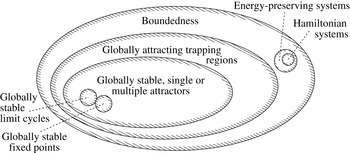
The difficulty of finding an appropriate Lyapunov function can partially be ascribed by the design goal, e.g. by ensuring the global stability of fixed points in the whole phase space. Instead, conditions for the existence of an arbitrary globally attractive solution are considered. In this paper, we focus on the existence of trapping regions employing Lyapunov’s direct method (Swinnerton-Dyer Reference Swinnerton-Dyer2000). Roughly stated, a trapping region is a domain in the state space such that each trajectory, once it has entered the trapping region, will remain inside the trapping region for all times (Meiss Reference Meiss2007). In the case of a (globally) attracting trapping region, all trajectories outside of the trapping region converge to the trapping region. The assumption of the existence of an attracting trapping region is connected with several other properties of dynamical systems (see figure 1). In the case that an attracting trapping region exists, the system dynamics is long-term bounded because the habitat of the long-term dynamics is represented by this trapping region. An existing (globally stable) single or multiple attractor must be embedded inside of an attracting trapping region.
Venn diagram of dynamical systems.

The existence of an attracting trapping region can be ensured via the existence of a function that is strictly of Lyapunov function type outside of a trapping region. As a well-known example, the existence of an attracting trapping region is shown for the Lorenz system (Swinnerton-Dyer Reference Swinnerton-Dyer2001). Further general findings can be traced back to Lorenz (Reference Lorenz1963), where the existence of monotonically attracting trapping regions is shown for linear–quadratic systems with negative definite linear term and energy-preserving quadratic term. We follow these hints to investigate long-term boundedness and to estimate the extent of existing attractors. In particular, we focus on the generality for the considered class of linear–quadratic dynamical systems and the simplicity of the construction of the respective Lyapunov functions.
This paper is structured as follows. In § 2, the class of the considered dynamical systems is defined. A criterion for long-term boundedness and existence of globally stable attractors is proposed in § 3. Analytical and numerical application results are given for the investigation of long-term boundedness of Galerkin systems for wall-bounded shear flows in § 4, and of Galerkin systems for the post-transient and transient dynamics of a two-dimensional cylinder wake flow in § 5. The Lorenz system is investigated in § 6. Algorithms and computational load associated with the criterion and alternatives are discussed in § 7. In § 8, the main findings are summarised and future directions are indicated. The proposed criterion is illustrated by a sample system fulfilling the criterion and examples for systems in which the criterion is violated in the first and third appendices A and C, respectively. The theorems of § 3 are proven in appendix B. In appendix D, potentials of the criterion for state stabilisation and for attractor control are illustrated.
2. Galerkin models of fluid flows
In this section, the considered class of dynamical systems is introduced. These systems naturally arise as Galerkin models of the incompressible Navier–Stokes equation in a steady domain
 ${\it\Omega}$
with stationary boundary conditions (see e.g. Holmes et al.
Reference Holmes, Lumley, Berkooz and Rowley2012). Galerkin models are typically extracted in two steps. First, a finite-dimensional Hilbert function subspace
 $\mathscr{H}$
is chosen. This subspace is spanned by space-dependent modes
 $\boldsymbol{u}_{i},~i=1,\dots ,N$
, which form an orthonormal basis in this Hilbert space. The flow
 $\boldsymbol{u}$
is modelled by a Galerkin approximation with a base flow
 $\boldsymbol{u}_{0}$
fulfilling stationary boundary conditions, and an expansion for the fluctuation
 $\boldsymbol{u}^{\prime }=\boldsymbol{u}-\boldsymbol{u}_{0}$
:
 $$\begin{eqnarray}\boldsymbol{u}({\bf\xi},t)=\boldsymbol{u}_{0}({\bf\xi})+\mathop{\sum }_{i=1}^{N}x_{i}(t)\,\boldsymbol{u}_{i}({\bf\xi}).\end{eqnarray}$$
The flow state is described by the time-dependent modal amplitudes
 $x_{i}$
. The spatial variables are denoted by
 ${\bf\xi}$
and the time by
 $t$
. The base flow
 $\boldsymbol{u}_{0}$
might represent a steady Navier–Stokes solution or mean flow. The main purpose for the introduction of the base flow is that (2.1) satisfies the boundary conditions for arbitrary choices of modal coefficients
 $x_{i}$
(Ladyz̆henskaya Reference Ladyz̆henskaya1963). The expansion modes
 $\boldsymbol{u}_{i},~i=1,\dots ,N$
, may arise from a proper orthogonal decomposition (POD) of snapshot data or from other mathematical considerations (Noack & Fasel Reference Noack and Fasel1994).
In the second step, a dynamical system is identified. At first, the Navier–Stokes equation is projected onto the Hilbert subspace
 $\mathscr{H}$
(see e.g. Noack et al.
Reference Noack, Morzyński and Tadmor2011). As result of the modelling process, a class of dynamical systems is considered, formulated in the vector space of the state variable
 $\boldsymbol{x}=[x_{1},\dots ,x_{N}]^{\text{T}}$
by
 $$\begin{eqnarray}\frac{\text{d}x_{i}}{\text{d}t}=c_{i}+\mathop{\sum }_{j=1}^{N}l_{ij}\,x_{j}+\mathop{\sum }_{j,k=1}^{N}q_{ijk}\,x_{j}\,x_{k},\end{eqnarray}$$
with the real numbers
 $c_{i}$
,
 $l_{ij}$
and
 $q_{ijk}$
, for
 $i,j,k=1,\dots ,N$
. Without loss of generality, the
 $q_{ijk}$
are assumed to be symmetric in the last two indices, i.e.
 $$\begin{eqnarray}q_{ijk}=q_{ikj},\quad i,j,k=1,\dots ,N.\end{eqnarray}$$
The quadratic term in (2.2) can be shown to be energy-preserving for a large class of boundary conditions. One example is stationary Dirichlet boundary conditions, because the no-slip condition for all modes
 $\boldsymbol{u}_{i}\equiv \mathbf{0}$
is implied for all modes at the boundary (see e.g. Rummler Reference Rummler2000). As well, the proof for periodic boundary conditions is straightforward (see e.g. McComb Reference McComb1991; Holmes et al.
Reference Holmes, Lumley, Berkooz and Rowley2012). The two boundary conditions may be combined, as in plane parallel Couette and Poiseuille channel flows (Rummler & Noske Reference Rummler and Noske1998) or in Hagen–Poiseuille flow (Boberg & Brosa Reference Boberg and Brosa1988). Moreover, by a fast decrease of the velocity magnitude for classes of open flows (two-dimensional cylinder wake flows and jets, three-dimensional round jets (Schlichting Reference Schlichting1968)), evidence of energy preservation of open flows is supported by vanishing surface integrals.
An energy-preserving quadratic term implies that the sums of the quadratic coefficients over index permutations are zero
 $$\begin{eqnarray}q_{ijk}+q_{ikj}+q_{jik}+q_{jki}+q_{kij}+q_{kji}=2q_{ijk}+2q_{jik}+2q_{kij}=0,\quad i,j,k=1,\dots ,N.\end{eqnarray}$$
This property is postulated for the class of dynamical systems discussed in this paper.
The energy-preserving quadratic term has an important effect on the evolution of the fluctuation energy
 $$\begin{eqnarray}K:=\frac{1}{2}\mathop{\sum }_{i=1}^{N}x_{i}^{2}\geqslant 0.\end{eqnarray}$$
If
 $\boldsymbol{u}_{0}$
is the mean flow, then
 $K$
denotes the standard turbulent kinetic energy (TKE) of statistical fluid mechanics. The time derivative of
 $K$
reads
 $$\begin{eqnarray}\frac{\text{d}K}{\text{d}t}=[\boldsymbol{{\rm\nabla}}_{\!\boldsymbol{x}}K]^{\text{T}}\,\frac{\text{d}\boldsymbol{x}}{\text{d}t}=\mathop{\sum }_{i=1}^{N}x_{i}\,f_{i}(\boldsymbol{x})=\mathop{\sum }_{i=1}^{N}c_{i}\,x_{i}+\mathop{\sum }_{i,j=1}^{N}l_{ij}\,x_{i}\,x_{j},\end{eqnarray}$$
i.e. the quadratic terms cancel each other out by (2.4).
Defining the vector
 $\boldsymbol{c}:=[c_{1},\dots ,c_{N}]^{\text{T}}$
and matrix
 $\unicode[STIX]{x1D647}:=[l_{ij}]_{i,j=1}^{N}$
, the evolution of
 $K$
is given in a simple vector–matrix notation via
 $$\begin{eqnarray}\frac{\text{d}K}{\text{d}t}=\boldsymbol{c}^{\text{T}}\boldsymbol{x}+\boldsymbol{x}^{\text{T}}\unicode[STIX]{x1D647}_{S}\,\boldsymbol{x},\end{eqnarray}$$
where the symmetric part
 $\unicode[STIX]{x1D647}_{S}:=\,(\unicode[STIX]{x1D647}+\unicode[STIX]{x1D647}^{\text{T}})/2$
of
 $\unicode[STIX]{x1D647}$
is introduced.
3. A sufficient criterion for long-term boundedness
In this section, a sufficient criterion for long-term boundedness of Galerkin systems is derived to exclude infinite blow-ups of the system state
 $\boldsymbol{x}(t)$
in finite or infinite periods of time. Via the criterion of theorem 1 below, the existence of monotonically attracting trapping regions is considered. For a generic class of Galerkin systems (2.2) with effective nonlinearity, it is shown that a globally stable attractor can exist only if there is a monotonically attracting trapping region. For further comprehension of the criterion, the reader might moreover consult the investigation of the sample system (A 1) for long-term boundedness, elaborated in appendix A.
For generalisation of Lyapunov’s direct method, we introduce monotonically attracting trapping regions. A trapping region
 $D\subseteq \mathbb{R}^{N}$
is a compact set, in which each trajectory remains once it has entered, i.e. from
 $\boldsymbol{x}(s)\in D$
it follows that
 $\boldsymbol{x}(t)\in D$
for all
 $t>s$
. A trapping region is termed (globally) monotonically attracting if an energy is strictly monotonically decreasing along all trajectories starting from an arbitrary state outside of
 $D$
. This implies that outside of the trapping region the energy possesses the mathematical properties of a strict Lyapunov function. For mathematical convenience and physical intuition, energy
 $K$
defined in (2.5) is generalised by
 $$\begin{eqnarray}K_{\boldsymbol{m}}:=\frac{1}{2}\Vert \boldsymbol{x}-\boldsymbol{m}\Vert ^{2}=\frac{1}{2}\mathop{\sum }_{i=1}^{N}(x_{i}-m_{i})^{2}.\end{eqnarray}$$
This is modulo factor
 $1/2$
the square of the Euclidean distance to an arbitrary but fixed state
 $\boldsymbol{m}$
measured in the Euclidean norm
 $\Vert \cdot \Vert =\sqrt{2K(\cdot )}$
. As candidates for trapping regions it is sufficient to consider closed balls
 $$\begin{eqnarray}B(\boldsymbol{m},R):=\{\boldsymbol{x}\in \mathbb{R}^{N}:\Vert \boldsymbol{x}-\boldsymbol{m}\Vert \leqslant R\}\end{eqnarray}$$
with centre
 $\boldsymbol{m}$
and radius
 $0<R<\infty$
. For later reference, these closed balls are also expressed in terms of translated coordinates
 $\boldsymbol{y}=\boldsymbol{x}-\boldsymbol{m}$
:
 $$\begin{eqnarray}B_{\boldsymbol{y}}(R):=\{\boldsymbol{y}\in \mathbb{R}^{N}:\Vert \boldsymbol{y}\Vert \leqslant R\}.\end{eqnarray}$$
Here, any closed ball containing
 $D$
as a subset is a monotonically attracting trapping region as well.
In Lorenz (Reference Lorenz1963), the existence of a monotonically attracting trapping region is shown for negative definiteness of the symmetric linear part
 $\unicode[STIX]{x1D647}_{S}$
of system (2.2). Then, the growth of
 $K=K_{\mathbf{0}}$
vanishes only on the surface of an ellipsoid
 $E$
, and is positive only in the interior of
 $E$
. After a finite time, the system state is trapped in the smallest closed ball
 $B$
with centre at the origin
 $\boldsymbol{y}=\mathbf{0}$
such that the ellipsoid
 $E$
is contained (only in the non-generic case, in which there is a stable fixed point at the intersection of the boundaries of
 $B$
and
 $E$
, it might take an infinite time to enter
 $B$
). Hence, the smallest monotonically attracting trapping ball is given by
 $B$
. The long-term behaviour of the system, represented, for example, by a globally stable attractor, is either part of the boundary without growth of
 $K_{\mathbf{0}}$
, or alternates between positive energy growth inside of
 $E$
and negative energy growth in
 $B\setminus E$
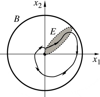
(see figure 2).
Principal sketch of boundedness of a solution of a Galerkin system (2.2) in a closed ball
 $B$
. The growth of energy to the origin is positive only inside of an ellipsoid
 $E$
.

To generalise this result, the origin is shifted to arbitrary
 $\boldsymbol{m}=[m_{1},\dots ,m_{N}]^{\text{T}}$
using the translation
 $$\begin{eqnarray}\boldsymbol{y}=\boldsymbol{x}-\boldsymbol{m},\end{eqnarray}$$
by which a transformation to new coordinates
 $\boldsymbol{y}$
is provided. To obtain a representation of the system in the new coordinates, the notation is kept simple, employing the following vector–matrix representation of (2.2),
 $$\begin{eqnarray}\frac{\text{d}\boldsymbol{x}}{\text{d}t}=\boldsymbol{c}+\unicode[STIX]{x1D647}\,\boldsymbol{x}+[\,\boldsymbol{x}^{\text{T}}\unicode[STIX]{x1D64C}^{(1)}\boldsymbol{x},\dots ,\,\boldsymbol{x}^{\text{T}}\unicode[STIX]{x1D64C}^{(N)}\boldsymbol{x}\,]^{\text{T}},\end{eqnarray}$$
using the symmetric matrices
 $\unicode[STIX]{x1D64C}^{({\it\alpha})}:=[q_{{\it\alpha}ij}]_{i,j=1}^{N}$
,
 ${\it\alpha}=1,\dots ,N$
. For the translated variable
 $\boldsymbol{y}=\boldsymbol{x}-\boldsymbol{m}$
, the dynamical system
 $$\begin{eqnarray}\frac{\text{d}\boldsymbol{y}}{\text{d}t}=\boldsymbol{d}+\unicode[STIX]{x1D63C}\,\boldsymbol{y}+[\,\boldsymbol{y}^{\text{T}}\unicode[STIX]{x1D64C}^{(1)}\boldsymbol{y},\dots ,\,\boldsymbol{y}^{\text{T}}\unicode[STIX]{x1D64C}^{(N)}\boldsymbol{y}\,]^{\text{T}}\end{eqnarray}$$
with
 $$\begin{eqnarray}\boldsymbol{d}:=\left(c_{i}+\mathop{\sum }_{j=1}^{N}l_{ij}m_{j}+\mathop{\sum }_{j,k=1}^{N}q_{ijk}m_{j}m_{k}\right)_{i=1}^{N}\end{eqnarray}$$
and
 $$\begin{eqnarray}\unicode[STIX]{x1D63C}:=\left(l_{ij}+\mathop{\sum }_{k=1}^{N}(q_{ijk}+q_{ikj})m_{k}\right)\end{eqnarray}$$
is obtained. Note that the symmetric part
 $\unicode[STIX]{x1D63C}_{S}$
of
 $\unicode[STIX]{x1D63C}$
can be represented as a linear combination of the symmetric part
 $\unicode[STIX]{x1D647}_{S}$
of
 $\unicode[STIX]{x1D647}$
and of the
 $\unicode[STIX]{x1D64C}^{(i)}$
,
 $$\begin{eqnarray}\unicode[STIX]{x1D63C}_{S}:=\frac{1}{2}(\unicode[STIX]{x1D63C}+\unicode[STIX]{x1D63C}^{\text{T}})=\unicode[STIX]{x1D647}_{S}-\mathop{\sum }_{i=1}^{N}m_{i}\,\unicode[STIX]{x1D64C}^{(i)},\end{eqnarray}$$
exploiting the symmetry properties (2.4) and (2.3). Invoking (2.6), the evolution of
 $K_{\boldsymbol{m}}=\sum _{i=1}^{N}y_{i}^{2}/2$
is given by
 $$\begin{eqnarray}\frac{\text{d}}{\text{d}t}K_{\boldsymbol{m}}=\boldsymbol{y}^{\text{T}}\unicode[STIX]{x1D63C}_{S}\,\boldsymbol{y}+\boldsymbol{d}^{\text{T}}\boldsymbol{y}=(\boldsymbol{x}-\boldsymbol{m})^{\text{T}}\unicode[STIX]{x1D63C}_{S}(\boldsymbol{x}-\boldsymbol{m})+\boldsymbol{d}^{\text{T}}(\boldsymbol{x}-\boldsymbol{m}),\end{eqnarray}$$
where
 $\boldsymbol{d}$
and
 $\unicode[STIX]{x1D63C}_{S}$
denote the constant and linear symmetric part of the transformed Galerkin system.
If all eigenvalues of
 $\unicode[STIX]{x1D63C}_{S}$
are negative after translation, i.e.
 $0>{\it\lambda}_{1}\geqslant \cdots \geqslant {\it\lambda}_{N}$
, then the observation of Lorenz (Reference Lorenz1963) is applicable. Every ball with origin
 $\boldsymbol{y}=\mathbf{0}$
at the centre, which contains the ellipsoid
 $E$
, is a monotonically attracting trapping region. This leads to the following theorem.
Theorem 1 (Monotonically attracting trapping regions).
Regarding the system (3.5), the following two statements are equivalent:
-
(a) There is a monotonically attracting trapping region.
-
(b) There is an
 $\boldsymbol{m}$
such that there are only negative eigenvalues
$0>{\it\lambda}_{1}\geqslant \cdots \geqslant {\it\lambda}_{N}$
of the symmetric linear part
$\unicode[STIX]{x1D63C}_{S}$
(3.9) of the shift-transformed system (3.6).



If these conditions are true, then
 $R_{m}=\sqrt{{\it\lambda}_{N}/{\it\lambda}_{1}}\,\Vert \boldsymbol{d}\Vert$
is a radius such that
 $B(\boldsymbol{m},R_{m})=B_{\boldsymbol{y}}(R_{m})$
is a monotonically attracting trapping region.
The theorem is proven in appendix B.
For a quantitative identification of the ellipsoid
 $E$
, invoke the diagonalisation
 $$\begin{eqnarray}\unicode[STIX]{x1D63C}_{S}=\unicode[STIX]{x1D64F}^{\text{T}}{\it\bf\Lambda}\unicode[STIX]{x1D64F}\end{eqnarray}$$
of the symmetric matrix
 $\unicode[STIX]{x1D63C}_{S}$
with the diagonal eigenvalue matrix
 ${\it\bf\Lambda}$
and the orthogonal matrix
 $\unicode[STIX]{x1D64F}$
comprising the eigenvectors; a transformation
 $$\begin{eqnarray}\boldsymbol{z}=\unicode[STIX]{x1D64F}\boldsymbol{y}\end{eqnarray}$$
is defined, preserving the energy
 $K_{\boldsymbol{m}}$
. Employing this coordinate transformation (rotation plus reflections) to the
 $\boldsymbol{y}$
formulation of (3.10), the energy growth is given by
 $$\begin{eqnarray}\frac{\text{d}}{\text{d}t}K_{\boldsymbol{m}}=\mathop{\sum }_{i=1}^{N}h_{i}\,z_{i}+{\it\lambda}_{i}\,z_{i}^{2}=\mathop{\sum }_{i=1}^{N}{\it\lambda}_{i}\,\left(z_{i}+\frac{h_{i}}{2{\it\lambda}_{i}}\right)^{2}-\mathop{\sum }_{i=1}^{N}\frac{h_{i}^{2}}{4{\it\lambda}_{i}},\end{eqnarray}$$
with the components
 $h_{i}$
of
 $\boldsymbol{h}\,:=\,\boldsymbol{d}\unicode[STIX]{x1D64F}^{\text{T}}$
.
For
 $\boldsymbol{d}=\mathbf{0}$
and hence
 $\boldsymbol{h}=\mathbf{0}$
, the energy is a strict Lyapunov function, because
 ${\it\lambda}_{i}<0$
,
 $i=1,\dots ,N$
, has been assumed. In addition, a globally stable fixed point is situated at the origin
 $\boldsymbol{y}=\boldsymbol{z}=\mathbf{0}$
. For
 $\boldsymbol{d}\neq \mathbf{0}$
and hence
 $\boldsymbol{h}\neq \mathbf{0}$
, the energy growth can be positive close to the origin. In more detail, the sign of the energy growth changes at the boundary of an ellipsoid
 $E$
, which is defined via
 $$\begin{eqnarray}\mathop{\sum }_{i=1}^{N}\frac{1}{{\it\alpha}_{i}^{2}}\left(z_{i}+\frac{h_{i}}{2{\it\lambda}_{i}}\right)^{2}=1\quad \text{with}~{\it\alpha}_{i}:=\frac{1}{2}\sqrt{\mathop{\sum }_{j=1}^{N}\frac{{\it\lambda}_{j}}{{\it\lambda}_{i}}\,h_{j}^{2}}.\end{eqnarray}$$
In the interior of the ellipsoid
 $E$
, the energy growth is positive. Outside of the ellipsoid the energy is decreasing. At the boundary, the energy stays constant. Note that the origin is situated at the boundary of the ellipsoid because it trivially solves (3.14). The half-axes
 ${\it\alpha}_{i}$
are directly proportional to the Euclidean norm of
 $\boldsymbol{h}$
and hence of
 $\boldsymbol{d}$
.
Revisiting theorem 1, at first a sufficient criterion for long-term boundedness is provided. The validity range of this criterion could be restricted by the nature of Lyapunov’s direct method or choice of the energy as Lyapunov function. From global stability analyses of stationary flows in pipes and channels, it is known that information loss may occur: employing the nonlinear stability based on Lyapunov’s direct method, the critical Reynolds numbers are underestimated by one order of magnitude (see e.g. Joseph Reference Joseph1976; Drazin & Reid Reference Drazin and Reid1981). For the criterion of theorem 1, it is at first only evidently known that, although long-term boundedness of a large class of systems is ensured, there might exist long-term bounded systems even with a globally stable fixed point that do not fit the condition of theorem 1. One class is given by Hamiltonian systems in which the energy
 $K_{\boldsymbol{m}}$
is preserved. Here,
 $\unicode[STIX]{x1D63C}_{S}=\mathbf{0}$
, because the distance to an
 $\boldsymbol{m}$
of the initial values remains constant for all times. All trajectories are embedded in invariant spaces, representing shells of constant distance around the centre. Hence the dynamics are bounded, but globally stable trapping regions or even a globally stable attractor do not exist. Another class is given from the linear system behaviour of (3.5) with vanishing nonlinear term
 $\unicode[STIX]{x1D64C}^{(i)}=\mathbf{0}$
,
 $i=1,\dots ,N$
,
 $\boldsymbol{c}=\mathbf{0}$
and a non-normal matrix
 $\unicode[STIX]{x1D647}$
. Here, an attracting behaviour can be accompanied with temporal energy growth as known from the theory of non-normal matrices (Trefethen & Embree Reference Trefethen and Embree2005). Even if there is a globally stable fixed point, the convergence of the trajectories can be non-monotonic with alternating increase and decrease of the distance to the fixed point.
To show the necessity implication of the criterion of theorem 1 for a large subclass of dynamical systems, a second theorem is derived. To define this subclass, the notion of an effective nonlinearity is introduced. The nonlinearity of system (3.5) is termed ‘effective’ if there is no non-trivial linear subspace in which the nonlinear term vanishes and where the trajectory given by the prevalent linear dynamics remains in this subspace for an infinite time horizon.
For systems with effective nonlinearity, the criterion of theorem 1 is equivalent to boundedness. This is formulated in the following theorem.
Theorem 2 (Necessity of the criterion).
Consider a system (3.5) with effective nonlinearity. If the system is long-term bounded, i.e. there are
 $T$
and
 $R$
such that
 $\Vert \boldsymbol{x}(t)\Vert <R$
for all
 $t>T$
, then there is a shift vector
 $\boldsymbol{m}$
such that the symmetric linear part
 $\unicode[STIX]{x1D63C}_{S}$
(3.9) of the shift-transformed system (3.6) is negative semidefinite.
This theorem is proven in appendix B. It should be noted that the unlikely special case, that
 $\unicode[STIX]{x1D63C}_{S}$
is negative semidefinite for one shift vector but never negative definite, is not separately discussed for simplicity of presentation.
In the complementary subclass of systems with at least one linear subspaces in which the system dynamics is reduced to linear behaviour, the above procedure for investigation of long-term boundedness has to be extended by linear analyses.
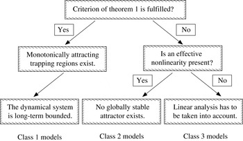
The results of this section culminate in the procedure sketched in figure 3, guiding the determination of the long-term behaviour of the Galerkin systems (2.2). To prove boundedness, an
 $\boldsymbol{m}$
has to be found, such that the largest eigenvalue of the respective
 $\unicode[STIX]{x1D63C}_{S}$
is positive. Otherwise, linear subspaces of the null space of the quadratic term have to be identified, in which a corresponding linear dynamics has to be investigated.
Decision tree diagram for long-term boundedness of linear–quadratic systems.

4. Long-term boundedness of Galerkin models for wall-bounded shear flows
Following the arguments of Lorenz (Reference Lorenz1963), which are generalised in the previous section, long-term boundedness of Galerkin models of fluid flows can be immediately seen from elementary considerations. For a demonstration, such results of three Galerkin models for wall-bounded shear flows are summarised, all representing flow mechanisms in Couette flows: the fourth-order models of Waleffe (Reference Waleffe1995), the eighth-order models derived in Waleffe (Reference Waleffe1997) and the ninth-order models of Moehlis, Faisst & Eckardt (Reference Moehlis, Faisst and Eckardt2004). These systems are of the form
 $$\begin{eqnarray}\frac{\text{d}\boldsymbol{x}}{\text{d}t}=\boldsymbol{c}-{\it\bf\Lambda}\,\boldsymbol{x}+[\,\boldsymbol{x}^{\text{T}}\unicode[STIX]{x1D64C}^{(1)}\boldsymbol{x},\dots ,\,\boldsymbol{x}^{\text{T}}\unicode[STIX]{x1D64C}^{(N)}\boldsymbol{x}\,]^{\text{T}},\end{eqnarray}$$
where
 ${\it\bf\Lambda}$
is a diagonal matrix with positive diagonal entries.
Following our arguments, only the energy-preservation property of the quadratic term has to be shown, which can be easily done. Although this result is known, it indicates that there is a class of fluid flows for which long-term boundedness of physical Galerkin models can easily be verified employing the criterion.
5. Long-term boundedness of Galerkin models for cylinder wake flows
In this section, we investigate the long-term boundedness of a hierarchy of Galerkin models for periodic cylinder wakes (Noack et al. Reference Noack, Afanasiev, Morzyński, Tadmor and Thiele2003). The considered systems include a three-dimensional mean-field system (§ 5.1), an eight-dimensional POD model (§ 5.2) and a nine-dimensional generalisation of this POD model with a stabilising shift mode (§ 5.3). The existence of a monotonically attracting trapping region is demonstrated analytically for the mean-field system, which is known to have a globally stable limit cycle. The corresponding existence is also numerically shown for the nine-dimensional model that generalises the mean-field system by inclusion of the second to fourth harmonics. The existence of a monotonically attracting trapping region is disproved for the eight-dimensional system, which has a locally stable limit cycle but also solutions converging to infinity. Thus, by the theorems of § 3, the dynamical behaviour suggested by preliminary investigations is proven.
5.1. On the long-term boundedness of a mean-field system
We consider a mean-field system for a soft onset of oscillatory fluctuations (Noack et al.
Reference Noack, Afanasiev, Morzyński, Tadmor and Thiele2003) in fluid flows. The state contains three coordinates:
 $x_{1}$
and
 $x_{2}$
describe the amplitude of the phase of the oscillatory fluctuation, and
 $x_{3}$
characterises the mean-field deformation. The origin
 $x_{1}=x_{2}=x_{3}=0$
corresponds to the steady solution. For simplicity, many parameters of the general mean-field model (see e.g. Noack et al.
Reference Noack, Morzyński and Tadmor2011) are set to zero or unity, following § 2.1 of Noack et al. (Reference Noack, Afanasiev, Morzyński, Tadmor and Thiele2003). Only the bifurcation parameter
 ${\it\mu}$
is left. The resulting mean-field system reads
 $$\begin{eqnarray}\displaystyle \frac{\text{d}x_{1}}{\text{d}t} & = & \displaystyle {\it\mu}x_{1}-x_{2}-x_{1}x_{3},\end{eqnarray}$$
 $$\begin{eqnarray}\displaystyle \frac{\text{d}x_{2}}{\text{d}t} & = & \displaystyle {\it\mu}x_{2}+x_{1}-x_{2}x_{3},\end{eqnarray}$$
 $$\begin{eqnarray}\displaystyle \frac{\text{d}x_{3}}{\text{d}t} & = & \displaystyle -x_{3}+x_{1}^{2}+x_{2}^{2}\end{eqnarray}$$
 ${\it\mu}<0$
), the system has a globally stable fixed point
 $x_{1}=x_{2}=x_{3}=0$
. For supercritical values (
 ${\it\mu}>0$
), these fixed points becomes unstable and all trajectories converge to the limit cycle
 $$\begin{eqnarray}x_{1}=\sqrt{{\it\mu}}\cos (t),\quad x_{2}=\sqrt{{\it\mu}}\sin (t),\quad x_{3}={\it\mu}\end{eqnarray}$$
modulo an irrelevant phase. This limit cycle represents vortex shedding (Noack et al. Reference Noack, Morzyński and Tadmor2011).
This differential equation system can be brought into the form (3.5) with
 $$\begin{eqnarray}\boldsymbol{c}=\left[\begin{array}{@{}c@{}}0\\ 0\\ 0\end{array}\right],\quad \unicode[STIX]{x1D647}=\left[\begin{array}{@{}ccc@{}}{\it\mu} & -1 & 0\\ 1 & {\it\mu} & 0\\ 0 & 0 & -1\end{array}\right]\end{eqnarray}$$
and
 $$\begin{eqnarray}\unicode[STIX]{x1D64C}^{(1)}=\left[\begin{array}{@{}ccc@{}}0 & 0 & -{\textstyle \frac{1}{2}}\\ 0 & 0 & 0\\ -{\textstyle \frac{1}{2}} & 0 & 0\end{array}\right],\quad \unicode[STIX]{x1D64C}^{(2)}=\left[\begin{array}{@{}ccc@{}}0 & 0 & 0\\ 0 & 0 & -{\textstyle \frac{1}{2}}\\ 0 & -{\textstyle \frac{1}{2}} & 0\end{array}\right],\quad \unicode[STIX]{x1D64C}^{(3)}=\left[\begin{array}{@{}ccc@{}}1 & 0 & 0\\ 0 & 1 & 0\\ 0 & 0 & 0\end{array}\right],\end{eqnarray}$$
with a real parameter
 ${\it\mu}>0$
.
As in the sample system (A 1), there are areas in which the amplitude of the oscillation in the
 $x_{1}{-}x_{2}$
plane grows while the
 $x_{3}$
direction has only negative distance growth. In fact, system (A 1) originated from the mean-field model (5.1) with
 ${\it\mu}=1$
. The first component
 $x_{1}$
in (A 1) corresponds to the amplitude
 $\sqrt{x_{1}^{2}+x_{2}^{2}}$
of the first two components in (5.1), and the second component
 $x_{2}$
corresponds to the component
 $x_{3}$
in (5.1).
The stabilisation of the limit cycle can be described by the Landau equation (Noack et al. Reference Noack, Afanasiev, Morzyński, Tadmor and Thiele2003). As for system (A 1), the boundedness of the mean-field dynamics cannot be derived from a quadratic Lyapunov function.
The criterion of theorem 1 can easily be satisfied. Consider the translation with
 $\boldsymbol{m}=[0,0,{\it\mu}+{\it\epsilon}]^{\text{T}}$
for an
 ${\it\epsilon}>0$
. Employing moreover (3.9), the symmetric part of the transformed system is derived to be
 $$\begin{eqnarray}\unicode[STIX]{x1D63C}_{S}=\left[\begin{array}{@{}ccc@{}}-{\it\epsilon} & 0 & 0\\ 0 & -{\it\epsilon} & 0\\ 0 & 0 & -1\end{array}\right]\!.\end{eqnarray}$$
The negative definiteness of
 $\unicode[STIX]{x1D63C}_{S}$
implies the existence of a monotonically attracting trapping region. Following theorem 1, one of these regions is given by the closed ball
 $B(\boldsymbol{m},R_{m})$
, where
 $R_{m}=({\it\mu}+{\it\epsilon})/\sqrt{{\it\epsilon}}$
. Hence, the trapping region will grow to infinity for
 ${\it\epsilon}\rightarrow 0$
. The limit cycle is situated inside of
 $B$
and at the boundary of the ellipsoid
 $E$
defined by (3.14), along which the energy
 $K_{\boldsymbol{m}}$
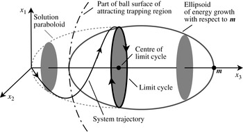
is constant. This is illustrated in figure 4. We employ that
 $\boldsymbol{m}$
lies on the
 $x_{3}$
-axis orthogonal to the limit cycle plane, and
 $K_{\boldsymbol{m}}$
is seen to remain constant on the limit cycle. The limit cycle is contained in the intersection set of the infinite number of ellipsoids, each defined by a positive parameter
 ${\it\epsilon}>0$
.
Solution behaviour of the system (5.1). The trajectories converge in spirals along the paraboloid (dashed light grey line) towards the globally stable limit cycle (thick solid black line), as exemplified by one representative (thin solid black line). For one
 $\boldsymbol{m}$
with a corresponding negative definite
 $\unicode[STIX]{x1D63C}_{S}$
, the trapping region of minimal radius (indicated by dot-dashed black line) is determined by the contained ellipsoid of positive energy growth (3.14) (thick solid dark grey line).

5.2. On the long-term boundedness of a POD Galerkin model
In Deane et al. (Reference Deane, Kevrekidis, Karniadakis and Orszag1991) and Noack et al. (Reference Noack, Afanasiev, Morzyński, Tadmor and Thiele2003), a Galerkin model for the cylinder wake flow is proposed employing the first eight modes from a POD. The post-transient dynamics of oscillatory laminar vortex shedding at a Reynolds number of
 $\mathit{Re}=100$
in the wake is accurately resolved by this model.
The eight-dimensional Galerkin system is given by the differential equation
 $$\begin{eqnarray}\frac{\text{d}x_{i}}{\text{d}t}=c_{i}+\mathop{\sum }_{j=1}^{8}l_{ij}x_{j}+\mathop{\sum }_{j,k=1}^{8}q_{ijk}x_{j}x_{k}.\end{eqnarray}$$
The energy-preservation property (2.4) is enforced for the quadratic term. The kinetic energy
 $K$
is produced in the first mode pair (
 $x_{1},x_{2}$
) with the same positive growth rate of energy. The other six modes form pairs of the same negative energy growth rate, consuming the energy transferred by the first pair. For initial conditions close to the projection of the Navier–Stokes attractor onto the eight-dimensional subspace, the post-transient dynamics is reproduced (Noack et al.
Reference Noack, Afanasiev, Morzyński, Tadmor and Thiele2003). Starting far from the limit cycle, also solutions that converge to infinity are numerically observed.
To test the criterion of theorem 1, the largest eigenvalue of the linear symmetric part
 $\unicode[STIX]{x1D63C}_{S}$
is minimised over a set of shift vectors
 $\boldsymbol{m}$
. The optimisation has been performed via a simulated annealing algorithm (see e.g. Gershenfeld Reference Gershenfeld2006) with random seeding in
 $\boldsymbol{m}\in [-100,100]^{8}$
. This interval contains the centre of the limit cycle and can be considered as very large, since it is almost two orders of magnitude larger than the radius of this limit cycle. Here
 $10^{4}$
initial conditions have been employed. The stopping criterion is given by the convergence of the largest eigenvalue with a computational accuracy of eight digits. The computations stop before the 100th temperature decrease is done. During each temperature stage,
 $10^{3}$
iterations are computed.
In all computations, the dynamics converge to a minimum of
 $0<{\it\lambda}_{1}\approx 0.013285$
of the largest eigenvalue of
 $\unicode[STIX]{x1D63C}_{S}$
, which indicates that the criterion cannot be fulfilled. This result indicates unboundedness of the solution, which is demonstrated by simulations of Noack et al. (Reference Noack, Afanasiev, Morzyński, Tadmor and Thiele2003) showing divergent behaviour of the system dynamics of (5.6) to infinity for some initial values. Also Deane et al. (Reference Deane, Kevrekidis, Karniadakis and Orszag1991) report fragile Galerkin system behaviour for a similar POD wake model. In fact, the fragility of the POD model for vortex shedding has inspired numerous enhancements of the reduced-order modelling method, e.g. a nonlinear eddy viscosity term (Cordier et al.
Reference Cordier, Noack, Daviller, Lehnasch, Tissot, Balajewicz and Niven2013), a stabilising spectral viscosity term (Sirisup & Karniadakis Reference Sirisup and Karniadakis2004), a stabilising linear term (Galletti et al.
Reference Galletti, Bruneau, Zannetti and Iollo2004), a stabilising additional shift mode (Noack et al.
Reference Noack, Afanasiev, Morzyński, Tadmor and Thiele2003), or the inclusion of Navier–Stokes constraints construction of generalised POD modes (Balajewicz et al.
Reference Balajewicz, Dowell and Noack2013).
5.3. On the long-term boundedness of a POD Galerkin model with shift mode
The eight-dimensional POD model of the previous section is stabilised by including an additional shift mode
 $\boldsymbol{u}_{9}$
in the Galerkin expansion following Noack et al. (Reference Noack, Afanasiev, Morzyński, Tadmor and Thiele2003, Reference Noack, Papas and Monkewitz2005). This shift mode
 $\boldsymbol{u}_{9}$
represents the normalised difference of mean flow and stationary solution. In addition, the base flow
 $\boldsymbol{u}_{0}$
is chosen to be the unstable steady solution so that the origin
 $\boldsymbol{x}=\mathbf{0}$
represents the fixed point of the Navier–Stokes dynamics. In the following, long-term boundedness of the resulting nine-mode Galerkin system is proven for all initial conditions.
The dynamical system (5.6) is generalised by additional terms on the right-hand sides and a new additional equation arising from the shift mode:
 $$\begin{eqnarray}\displaystyle \frac{\text{d}x_{i}}{\text{d}t} & = & \displaystyle \underbrace{c_{i}+\mathop{\sum }_{j=1}^{8}l_{ij}x_{j}+\mathop{\sum }_{j,k=1}^{8}q_{ijk}x_{j}x_{k}}_{\text{terms from the eight-mode system (5.4)}}\nonumber\\ \displaystyle & & \displaystyle +\,\underbrace{l_{i9}x_{9}+\mathop{\sum }_{k=1}^{8}q_{i9k}x_{9}x_{k}+\mathop{\sum }_{j=1}^{8}q_{ij9}x_{j}x_{9}+q_{i99}x_{9}^{2}}_{\text{additional shift mode terms}},\quad i=1,\dots ,8,\end{eqnarray}$$
 $$\begin{eqnarray}\frac{\text{d}x_{9}}{\text{d}t}=c_{9}+\mathop{\sum }_{j=1}^{9}l_{9j}x_{j}+\mathop{\sum }_{j,k=1}^{9}q_{9jk}x_{j}x_{k}.\end{eqnarray}$$
In the following, we prove long-term boundedness of the nine-mode Galerkin system with the criterion of theorem 1. Learning from the mean-field model, only translations (3.4) along the mean-field axis are considered, i.e.
 $\boldsymbol{m}=$
 $(0,0,0,0,0,0,0,0,{\it\alpha})^{\text{T}}$
with
 ${\it\alpha}>0$
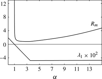
. Figure 5 visualises the situation at
 ${\it\alpha}\approx 1$
. There is a change of the sign of the largest eigenvalue of
 $\unicode[STIX]{x1D63C}_{S}$
from being positive to negative at
 ${\it\alpha}\approx 1$
. By the translation, the largest eigenvalue decreases initially linearly with
 ${\it\alpha}$
. After some value of
 ${\it\alpha}$
, this largest eigenvalue remains negative and constant due to other eigenvalues that are not affected by the translation. Thus, the largest eigenvalue of
 $\unicode[STIX]{x1D63C}_{S}$
remains constant for larger
 ${\it\alpha}$
.
Visualisation of the criterion of theorem 1 for long-term boundedness of the nine-mode cylinder wake Galerkin system (5.7). At the left side, the largest eigenvalue
 ${\it\lambda}_{1}$
of
 $\unicode[STIX]{x1D63C}_{S}$
of the shifted system (3.6) and the estimated radius
 $R_{m}$
of the globally attracting trapping ball
 $B$
described in this theorem are shown, for several shift vectors
 $\boldsymbol{m}=(0,0,0,0,0,0,0,0,{\it\alpha})^{\text{T}}$
with
 ${\it\alpha}>0$
. At the right side a section is zoomed to identify the minimum of
 $R_{m}\approx 0.82$
at
 ${\it\alpha}\approx 3.0$
.

Moreover, the simulated annealing procedure has been employed as described in the last subsection, but employing the stopping criterion, that the largest eigenvalue of
 $\unicode[STIX]{x1D63C}_{S}$
is lower than
 $-10^{-3}$
. All computations stop before the 50th temperature decrease step has been done. It has to be noted that only a fraction of the computational load is necessary, because with only one of these computations the existence of the desired
 $\boldsymbol{m}$
is ensured.
In conclusion, there exists an
 $\boldsymbol{m}$
for which
 $\unicode[STIX]{x1D63C}_{S}$
is negative definite. Thus, the nine-mode Galerkin system is shown to be long-term bounded because a monotonically attracting trapping region must exist according to theorem 1.
Furthermore, it is shown in figure 5 that there is a minimum of the volume of the trapping region for a certain
 $\boldsymbol{m}$
as indicated by the curve of the estimated radius
 $R_{m}$
of the trapping region. So this
 $\boldsymbol{m}$
indicates the centre along the considered line, where the attractor can be embedded in the smallest monotonically trapping region ball. For smaller or larger values of
 ${\it\alpha}$
, the centre
 $\boldsymbol{m}$
is situated further away from the attractor and thus the corresponding
 $R_{m}$
is larger.
6. Long-term boundedness of the Lorenz system
The existence of a monotonically attracting trapping region is demonstrated for Galerkin systems (2.2) with stable fixed point behaviour of the sample system (A 1) and the stable periodic limit cycle dynamics of system (5.1). In this section and appendix C, more complex examples are considered. We start with the well-known Lorenz system
 $$\begin{eqnarray}\displaystyle \frac{\text{d}x_{1}}{\text{d}t} & = & \displaystyle -{\it\sigma}x_{1}+{\it\sigma}x_{2},\end{eqnarray}$$
 $$\begin{eqnarray}\displaystyle \frac{\text{d}x_{2}}{\text{d}t} & = & \displaystyle {\it\rho}x_{1}-x_{2}-x_{1}x_{3},\end{eqnarray}$$
 $$\begin{eqnarray}\displaystyle \frac{\text{d}x_{3}}{\text{d}t} & = & \displaystyle -{\it\beta}x_{3}+x_{1}x_{2},\end{eqnarray}$$
 ${\it\sigma}$
,
 ${\it\rho}$
and
 ${\it\beta}$
. By these equations a Galerkin system is provided, modelling the Overbeck–Boussinesq system as detailed by Saltzman (Reference Saltzman1962) and Lorenz (Reference Lorenz1963). The Lorenz system is of the form (3.5) with
 $\boldsymbol{c}=\mathbf{0}$
,
 $\unicode[STIX]{x1D64C}^{(1)}=\mathbf{0}$
and
 $$\begin{eqnarray}\unicode[STIX]{x1D647}=\left[\begin{array}{@{}ccc@{}}-{\it\sigma} & {\it\sigma} & 0\\ {\it\rho} & -1 & 0\\ 0 & 0 & -{\it\beta}\end{array}\right],\quad \unicode[STIX]{x1D64C}^{(2)}=\left[\begin{array}{@{}ccc@{}}0 & 0 & -{\textstyle \frac{1}{2}}\\ 0 & 0 & 0\\ -{\textstyle \frac{1}{2}} & 0 & 0\end{array}\right],\quad \unicode[STIX]{x1D64C}^{(3)}=\left[\begin{array}{@{}ccc@{}}0 & {\textstyle \frac{1}{2}} & 0\\ {\textstyle \frac{1}{2}} & 0 & 0\\ 0 & 0 & 0\end{array}\right]\!.\end{eqnarray}$$
In particular, the quadratic term is energy preserving. For Lorenz’s choice of parameters,
 $$\begin{eqnarray}{\it\sigma}=10,\quad {\it\rho}=28,\quad {\it\beta}={\textstyle \frac{8}{3}},\end{eqnarray}$$
the solution is characterised by a strange attractor. However, it is known that the solution is long-term bounded. A trapping region of ellipsoidal form can be found via a Lyapunov function (Swinnerton-Dyer Reference Swinnerton-Dyer2001).
Because there are positive and negative eigenvalues of
 $\unicode[STIX]{x1D647}_{S}$
, there exist directions of positive and negative energy growth
 $K$
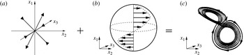
. However, via the quadratic term the trajectories are deflected from directions of positive energy growth to directions of negative energy growth, stabilising the resulting strange attractor (see figure 6).
Fields of the symmetric part of (a) the linear term and (b) the quadratic term, and (c) the strange attractor of the Lorenz system (6.1) for Lorenz’s choice of system parameters.

The directions of energy growth and the symmetry axes of the quadratic term do not coincide. The dynamics of the system is dominated by the quadratic term in the case of large deviations from the origin
 $\boldsymbol{x}=\mathbf{0}$
and far enough from fixed points of the quadratic term at the two poles and the equator. Hence, the boundedness of the system is determined by the accumulation of energy growth along the trajectories of the quadratic term crossing areas of negative and positive growth. The set of points with a vanishing quadratic term has to be investigated separately, leading to an investigation of the linear term.
In the following, long-term boundedness is shown with the criterion of theorem 1. After the translation employing
 $\boldsymbol{m}=[0,0,{\it\rho}+{\it\sigma}]^{\text{T}}$
and invoking (3.9), the symmetric part of the transformed system is equal to
 $$\begin{eqnarray}\unicode[STIX]{x1D63C}_{S}=\left[\begin{array}{@{}ccc@{}}-{\it\sigma} & 0 & 0\\ 0 & -1 & 0\\ 0 & 0 & -{\it\beta}\end{array}\right]\!.\end{eqnarray}$$
The negative definiteness of the matrix
 $\unicode[STIX]{x1D63C}_{S}$
proves the existence of a monotonically attracting trapping region. Following theorem 1 further, one of these regions is given by the closed ball
 $B(\boldsymbol{m},R_{m})$
with
 $R_{m}={\it\beta}({\it\rho}+{\it\sigma})/\sqrt{{\it\sigma}}$
in the case of
 ${\it\sigma}>{\it\beta}>1$
. For Lorenz’s choice of parameters (6.3), the trapping region is given by
 $B(\boldsymbol{m},R_{m})\approx B([0,0,38]^{\text{T}},32)$
. Hence, the complete strange attractor is situated inside of the ball
 $B$
. It can be shown that the Lorenz system represents a prototype of the dynamics illustrated in figure 2 via further computation of the ellipsoid
 $E$
using (3.14). For large times the trajectories of the Lorenz system push through the boundary of the ellipsoid and are alternately repelling from and attracting to
 $\boldsymbol{m}$
.
7. Discussion
In this section, the algorithm and computational load associated with the criterion and alternatives are discussed. At the end, a procedure is provided to discriminate between long-term boundedness and unboundedness.
At first, to validate the criterion of theorem 1,
 $N$
components of
 $\boldsymbol{m}$
have to be found such that the
 $N$
eigenvalues of
 $\unicode[STIX]{x1D63C}_{S}$
are negative. Analytically this can usually only be done for low dimensions
 $N\leqslant 4$
, if the negative definiteness cannot be seen by mathematical or physical evidence.
As a simpler perspective, only the largest eigenvalue might be considered. Invoking (3.9) and the known continuous dependence of the largest eigenvalue of
 $\unicode[STIX]{x1D63C}_{S}$
on the matrix elements (see e.g. Horn & Johnson Reference Horn and Johnson2013), the largest eigenvalue depends continuously on the components of
 $\boldsymbol{m}$
. Hence, for a long-term bounded system, there is a non-zero Lebesgue measure of the set of all
 $\boldsymbol{m}$
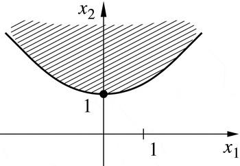
fulfilling the criterion. Moreover, this set is usually bounded by a piecewise polynomial curve, as illustrated for the sample example (A 1) in figure 7. By these regularity properties preconditions are provided for the successful application of numerical optimisation, e.g. by simulated annealing algorithms (see e.g. Gershenfeld Reference Gershenfeld2006) for minimisation of the first eigenvalue or, equivalently, to the solution of the inf–sup problem
 $$\begin{eqnarray}\inf _{\boldsymbol{m}}\sup _{\Vert \boldsymbol{y}\Vert =1}\,\boldsymbol{y}^{\text{T}}\left(\unicode[STIX]{x1D647}_{S}-\mathop{\sum }_{i=1}^{N}m_{i}\unicode[STIX]{x1D64C}^{(i)}\right)\boldsymbol{y}.\end{eqnarray}$$
One example is the simulated annealing algorithm employed in § 5.3 to prove boundedness.


The knowledge about a bounded trajectory determined by an integration of the system can supply the search for an
 $\boldsymbol{m}$
fulfilling the criterion – as indicated by the proof of theorem 2, the desired
 $\boldsymbol{m}$
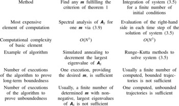
might be situated in a neighbourhood of the respective mean value. However, even a finite number of computed bounded trajectories usually do not prove long-term boundedness, whereas by the criterion the long-term boundedness of all trajectories is shown. A comparison is provided in table 1. Indeed, the computational load to search for an
 $\boldsymbol{m}$
fulfilling the criterion is similar to one integration of the system.
Algorithmic comparison between criterion of theorem 1 and system integration.

To prove unboundedness, it has to be shown that the criterion is not fulfilled for any
 $\boldsymbol{m}$
and there is an effective nonlinearity. Here, usually it is more efficient to find an unbounded trajectory of the system via integration of the system for several initial conditions. Alternatively, this problem might also be solved based on a generalisation of the Lyapunov function with higher-order terms.
Invoking theorem 2 in addition, it is clear that the choice of kinetic energy as Lyapunov function can always be employed to show long-term boundedness of the considered Galerkin systems. However, the energy function is a Lyapunov function only outside of an ellipsoid. To ensure asymptotic stability of a fixed point, the choice of the energy can be too restrictive. This is known, for example, from the theory of global stability of fluid flows (see e.g. Joseph Reference Joseph1976). The finding of a ‘background flow’ representing the coordinate shift (3.4) might remedy the restrictiveness of the energy function but is not necessarily enough for the proof (Doering & Constantin Reference Doering and Constantin1994). A promising approach of the construction of less restrictive Lyapunov functions is pursued by Goulart & Chernyshenko (Reference Goulart and Chernyshenko2012) and Chernyshenko et al. (Reference Chernyshenko, Goulart, Huang and Papachristodoulou2014) based on the polynomial sum of squares approach of Parrilo (Reference Parrilo2003).
To conclude, a procedure is suggested to discriminate between long-term bounded and unbounded Galerkin models of fluid flows. This procedure is based on mean-field modelling results and energy flow analyses of Noack et al. (Reference Noack, Afanasiev, Morzyński, Tadmor and Thiele2003, Reference Noack, Papas and Monkewitz2005), where the models of § 5 represents the paradigms. The procedure is described as follows:
-
(a) Compute a steady solution. Find a fixed point of the considered system and choose the system (3.5) based on that fixed point as origin
$\boldsymbol{x}=\mathbf{0}$
. If
$\unicode[STIX]{x1D647}_{S}$
is negative definite, long-term boundedness is shown. Otherwise continue with the unstable fixed point by which an unstable stationary flow is represented. -
(b) Integrate an unsteady solution. Integrate the system for an initial condition. If the dynamics diverges to infinity, unboundedness of the system is ensured. Otherwise compute the mean value
$\boldsymbol{x}_{m}$
of the known trajectory. -
(c) Search in the direction of the ‘shift mode’. Choose
$\boldsymbol{m}={\it\alpha}\boldsymbol{x}_{m}$
and vary
${\it\alpha}$
to find an
$\boldsymbol{m}$
such that the largest eigenvalue of the corresponding
$\unicode[STIX]{x1D63C}_{S}$
is negative. Following mean-field arguments, the production of total kinetic energy at the base flow generally decreases linearly with increasing
${\it\alpha}$
. This leads to a net dissipation indicating a negative definite linear term.


Although this procedure is physically plausible, no mathematical guarantee of its success can be offered. Alternatively, a search in the full state space may be performed.
8. Conclusions and future directions
We consider linear–quadratic dynamical systems and propose a criterion that is sufficient for long-term boundedness and necessary for globally stable attractor behaviour. For the first time, a straightforward procedure (see figure 3) can identify control-oriented Galerkin models of a generic class with quadratic nonlinearity. The key enabler is a generalisation of Lyapunov’s direct method for identification of monotonically attracting trapping regions. These regions represent a more accessible property than the attractor property: the existence of monotonically attracting trapping regions is based solely on eigenvalue computations of linear combinations of system intrinsic matrices.
One distinct benefit is given for the model calibration and model reduction: non-divergent systems can be identified a priori. One can avoid the computational burden of integration of the dynamical systems needed for a comprehensive set of system parameters and a large set of initial conditions to indicate long-term boundedness of the system.
Similarly, control laws that may lead to divergent system behaviour can be rejected a priori. A straightforward control design is enabled via the design of monotonically attracting trapping regions. In the appendix D, the respective control design is detailed for state stabilisation and for attractor control.
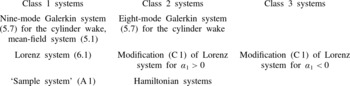
The criterion is applied to reduced-order models like the Galerkin models for wall-bounded shear flows (Waleffe Reference Waleffe1995, Reference Waleffe1997; Moehlis et al. Reference Moehlis, Faisst and Eckardt2004), the Galerkin models for a cylinder wake (Noack et al. Reference Noack, Afanasiev, Morzyński, Tadmor and Thiele2003), the Lorenz system (Saltzman Reference Saltzman1962; Lorenz Reference Lorenz1963), and its modification to show long-term boundedness or indicate unboundedness (see table 2).
Classification of the investigated dynamical systems employing the categories introduced in figure 3.

The proposed methods for showing long-term boundedness are generalisable to Galerkin systems of larger dimensions in a straightforward manner. Such systems may originate, for instance, from computational fluid dynamics. The numerical realisation of the criterion is only restricted by the current state of the art of the numerical linear algebra and multidimensional optimisation.
Acknowledgements
The authors acknowledge the support of the Deutsche Forschungsgemeinschaft (DFG) under grants SCHL 586/2-1, SCHL 586/1-1, NO 258/2-3 and NO 258/1-1 as well as the funding and excellent working conditions of the Chaire d’Excellence ‘Closed-loop control of turbulent shear flows using reduced-order models’ (TUCOROM) of the French Angence Nationale de la Recherche (ANR) hosted by Institut PPRIME. We appreciate valuable stimulating discussions with M. Abel, S. Chernyshenko, L. Cordier, T. Duriez, E. Kaiser, M. Morzyński, R. Niven, V. Parezanovic, R. Radespiel, R. Semaan, J. Sesterhenn, M. Segond and A. Spohn. Moreover, we thank the referees for insightful suggestions. We are grateful for outstanding computer and software support from M. Franke and L. Oergel.
Appendix A. A simple example illustrating the derived criterion
In this appendix, a simple example is worked out to illustrate the energy limiting mechanism and an application of the derived criterion of theorem 1.
The two-dimensional system
 $$\begin{eqnarray}\displaystyle & & \displaystyle \frac{\text{d}x_{1}}{\text{d}t}=x_{1}-x_{1}x_{2},\end{eqnarray}$$
 $$\begin{eqnarray}\displaystyle & & \displaystyle \frac{\text{d}x_{2}}{\text{d}t}=-x_{2}+x_{1}^{2}\end{eqnarray}$$
 $\unicode[STIX]{x1D647}_{S}=\unicode[STIX]{x1D647}=\left[\begin{array}{@{}cc@{}}1 & 0\\ 0 & -1\end{array}\right]$
of the two-dimensional system, the direction
 $[1,0]^{\text{T}}$
with positive energy growth and the direction
 $[0,1]^{\text{T}}$
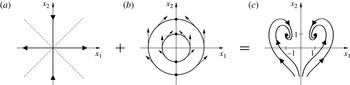
with negative energy growth are obtained (see figure 8). The field of the quadratic term deflects the trajectories from directions of growing energy into the directions of shrinking energy. The interaction of the unstable linear and the energy-preserving quadratic terms leads to a bounded dynamics. All trajectories are attracted by one of the stable fixed points
 $[-1,1]^{\text{T}}$
,
 $[1,1]^{\text{T}}$
, or along the abscissa to the origin
 $\boldsymbol{x}=\mathbf{0}$
, which represents an unstable fixed point. There is no quadratic Lyapunov function by which the convergence to one of the stable fixed points can be proven a priori. The Lyapunov function does not even exist in the corresponding open half-planes of attraction. The energy is increasing or decreasing depending on the location of the state. There are phase-space areas of positive or negative energy growth. If the dynamics along the trajectory is dominated by negative energy growth, the system state is attracted, for example, to fixed points as in system (A 1). If the dynamics is dominated by positive energy growth, the trajectories may diverge to infinity.
Fields of (a) the linear term and (b) the quadratic term, and (c) the stable fixed point behaviour of system (A 1).

Employing
 $\boldsymbol{m}=[0,2]^{\text{T}}$
in (3.4), the sample system (A 1) is given for the shifted coordinates by
 $$\begin{eqnarray}\displaystyle \frac{\text{d}y_{1}}{\text{d}t} & = & \displaystyle -y_{1}-y_{1}y_{2},\end{eqnarray}$$
 $$\begin{eqnarray}\displaystyle \frac{\text{d}y_{2}}{\text{d}t} & = & \displaystyle -2-y_{2}+y_{1}^{2},\end{eqnarray}$$
 $\boldsymbol{x}=\boldsymbol{m}$
, i.e.
 $\boldsymbol{y}=\mathbf{0}$
,
 $$\begin{eqnarray}\frac{\text{d}}{\text{d}t}K_{\boldsymbol{m}}=-2y_{2}-y_{1}^{2}-y_{2}^{2}.\end{eqnarray}$$
Hence, the energy is growing only in a bounded domain defined by the interior of the circle given by
 $y_{1}^{2}+(y_{2}+1)^{2}<1$
. If
 $K_{\boldsymbol{m}}$
is large, it will decrease and the trajectories cannot escape each circle
 $B$
with the origin at the centre in which the bounded domain of energy growth is contained. In conclusion, the long-term dynamics of the shifted system and consequently of the system (A 1) are bounded. Outside of each
 $B$
, the energy
 $K_{\boldsymbol{m}}$
represents a strict Lyapunov function and thus Lyapunov’s direct method is effective. Inside of
 $B$
, the energy
 $K_{\boldsymbol{m}}$
can grow and thus Lyapunov’s direct method cannot be applied.
As a first example of an application of the criterion of theorem 1, we show the existence of a monotonically attracting trapping region for the system (A 1). It can be written in the form of (3.5) with
 $$\begin{eqnarray}\boldsymbol{c}=\left[\begin{array}{@{}c@{}}0\\ 0\end{array}\right],\quad \unicode[STIX]{x1D647}=\left[\begin{array}{@{}cc@{}}1 & 0\\ 0 & -1\end{array}\right],\quad \unicode[STIX]{x1D64C}^{(1)}=\left[\begin{array}{@{}cc@{}}0 & -{\textstyle \frac{1}{2}}\\ -{\textstyle \frac{1}{2}} & 0\end{array}\right],\quad \unicode[STIX]{x1D64C}^{(2)}=\left[\begin{array}{@{}cc@{}}-1 & 0\\ 0 & 0\end{array}\right]\!.\end{eqnarray}$$
Considering the translation with
 $\boldsymbol{m}=[0,2]^{\text{T}}$
, and invoking (3.9), the symmetric part of the transformed system is
 $$\begin{eqnarray}\unicode[STIX]{x1D63C}_{S}=\left[\begin{array}{@{}cc@{}}-1 & 0\\ 0 & -1\end{array}\right]\!.\end{eqnarray}$$
By the negative definiteness of
 $\unicode[STIX]{x1D63C}_{S}$
, the existence of a monotonically attracting trapping region is shown. One of these regions is given by the closed ball
 $B_{\boldsymbol{y}}(2)$
in the
 $\boldsymbol{y}$
coordinates (see (3.3)) and equivalently by
 $B(\boldsymbol{m},2)$
in the
 $\boldsymbol{x}$
coordinates (see (3.2)). All solutions given by the stable and unstable fixed points are situated inside of
 $B$
and at the boundary of the ellipsoid
 $E$
defined by (3.14), along which the energy
 $K_{\boldsymbol{m}}$
is maintained.
Appendix B. Proofs of the theorems
B.1. Proof of theorem 1
As shown by Lorenz (Reference Lorenz1963), there is a monotonically attracting trapping region for the shifted system, if all eigenvalues of
 $\unicode[STIX]{x1D63C}_{S}$
are negative, i.e.
 $0>{\it\lambda}_{1}\geqslant \cdots \geqslant {\it\lambda}_{N}$
. In this case the energy evolution equation is transformed to (3.13) employing the rotation of the coordinate system to the principal axes. Hence, the domain of energy growth is identified to be inside of the ellipsoid given by (3.14). Consider the estimate
 $$\begin{eqnarray}{\it\alpha}_{i}\leqslant \frac{1}{2}\sqrt{\frac{{\it\lambda}_{N}}{{\it\lambda}_{1}}}\,\Vert \boldsymbol{d}\Vert ,\end{eqnarray}$$
invoking the definition (3.14) of the half-axes
 ${\it\alpha}_{i}$
. Then the radius of such a ball, not necessarily the infimum amongst such radii, is given by
 $R_{m}=\sqrt{{\it\lambda}_{N}/{\it\lambda}_{1}}\,\Vert \boldsymbol{d}\Vert$
.
On the other hand, given a monotonically attracting trapping region, the distance of every state
 $\boldsymbol{x}$
outside the trapping region to a state
 $\boldsymbol{m}$
inside of the trapping region is monotonically decreasing by definition. This is only true if the right-hand side of the power balance equation (3.10) is negative for this
 $\boldsymbol{m}$
for any
 $\boldsymbol{x}$
with large distance from
 $\boldsymbol{m}$
, i.e. if the
 $K_{\boldsymbol{m}}$
is large enough. By symmetry considerations this proves that all eigenvalues of
 $\unicode[STIX]{x1D63C}_{S}$
are negative.
B.2. Proof of theorem 2
Because of the assumed long-term boundedness of the system, the ensemble average
 $\langle \cdot \rangle$
is defined. The ensemble average of any observable
 $\boldsymbol{g}$
is given by
 $$\begin{eqnarray}\langle \boldsymbol{g}\rangle =\int _{\mathbb{R}^{N}}\boldsymbol{g}{\it\rho}(\boldsymbol{x})\text{d}\boldsymbol{x},\end{eqnarray}$$
with the invariant (probability) density
 ${\it\rho}(\boldsymbol{x})$
of the dynamical system (3.5) representing the probability of the system state
 $\boldsymbol{x}$
for large times assuming uniform distribution of initial conditions (see e.g. Kryloff & Bogoliouboff Reference Kryloff and Bogoliouboff1935; Manneville Reference Manneville2004; Holmes et al.
Reference Holmes, Lumley, Berkooz and Rowley2012).
An
 $\tilde{\boldsymbol{m}}$
can be found such that, for the transformed system (3.6) with
 $\boldsymbol{m}=\tilde{\boldsymbol{m}}$
, the ensemble average is zero,
 $\langle \boldsymbol{y}\rangle =\mathbf{0}$
. Let
 $\tilde{\boldsymbol{c}}=\boldsymbol{d}$
,
 $\tilde{\unicode[STIX]{x1D647}}=\unicode[STIX]{x1D63C}$
and
 $\tilde{\unicode[STIX]{x1D647}}_{S}:=\unicode[STIX]{x1D63C}_{S}$
be defined as constant term, linear term and its symmetric part of the shifted system, respectively. Moreover, let the reference coordinate system
 $\boldsymbol{x}$
of the original system (3.5) be transformed by
 $\tilde{\boldsymbol{x}}=\boldsymbol{x}-\tilde{\boldsymbol{m}}$
. Then the obtained system is of the form (3.5). For simplicity of representation, the tildes over the variables are dropped.
Hence, without loss of generality, systems of the form (3.5) can be considered with a zero ensemble average
 $\langle \boldsymbol{x}\rangle =\mathbf{0}$
of the dynamics. While the existence of such a reference system is ensured, the constant and linear parts of this reference system are usually a priori unknown. It will be shown that
 $\tilde{\unicode[STIX]{x1D647}}_{S}$
is negative semidefinite and thus the theorem holds.
A reformulation of the corresponding transformed system (3.6) is considered. Let
 $r:=\Vert \boldsymbol{y}\Vert >0$
be the amplitude (radius) of the state and
 $\boldsymbol{w}:=\boldsymbol{y}/r$
the ‘generalised phase’ (direction) on the unit ball
 $\partial B_{\boldsymbol{y}}(1)$
. It yields, with the identity matrix
 $\unicode[STIX]{x1D644}$
,
 $$\begin{eqnarray}\displaystyle \frac{\text{d}\boldsymbol{w}}{\text{d}t} & = & \displaystyle \frac{1}{r}(\boldsymbol{d}-(\boldsymbol{d}^{\text{T}}\boldsymbol{w})\boldsymbol{w})+(\unicode[STIX]{x1D63C}-(\boldsymbol{w}^{\text{T}}\unicode[STIX]{x1D63C}_{S}\boldsymbol{w})\unicode[STIX]{x1D644})\boldsymbol{w}\nonumber\\ \displaystyle & & \displaystyle +\,r[\,\boldsymbol{w}^{\text{T}}\unicode[STIX]{x1D64C}^{(1)}\boldsymbol{w},\dots ,\,\boldsymbol{w}^{\text{T}}\unicode[STIX]{x1D64C}^{(N)}\boldsymbol{w}\,]^{\text{T}},\end{eqnarray}$$
 $$\begin{eqnarray}\displaystyle \frac{\text{d}r}{\text{d}t} & = & \displaystyle \boldsymbol{d}^{\text{T}}\boldsymbol{w}+r\boldsymbol{w}^{\text{T}}\unicode[STIX]{x1D63C}_{S}\boldsymbol{w}.\end{eqnarray}$$
 $\boldsymbol{m}=\mathbf{0}$
, it is known that
 $\langle \boldsymbol{y}\rangle =\mathbf{0}$
. Given a long-term bounded system, i.e.
 $\Vert \boldsymbol{y}+\boldsymbol{m}\Vert <R$
for large
 $t$
, then the correlation matrix can be chosen as
 $$\begin{eqnarray}\unicode[STIX]{x1D652}_{\boldsymbol{m}}:=[\langle w_{i}w_{j}\rangle ]_{i,j=1}^{N}\approx \boldsymbol{v}\boldsymbol{v}^{\text{T}},\quad \text{for each}~\boldsymbol{v}\in B(0,1)\end{eqnarray}$$
because
 $\boldsymbol{m}=\Vert \boldsymbol{m}\Vert \boldsymbol{v}$
can be selected for arbitrary direction
 $\boldsymbol{v}$
and arbitrary large amplitude
 $\Vert \boldsymbol{m}\Vert$
. In the following, systems with large amplitudes
 $\Vert \boldsymbol{m}\Vert$
are considered.
For the considered class of effective nonlinearity, the constant and linear term of the phase equation (B 3a
) can be neglected for large
 $r$
,
 $$\begin{eqnarray}\frac{\text{d}\boldsymbol{w}}{\text{d}t}=r[\boldsymbol{w}^{\text{T}}\unicode[STIX]{x1D64C}^{(1)}\boldsymbol{w},\dots ,\,\boldsymbol{w}^{\text{T}}\unicode[STIX]{x1D64C}^{(N)}\boldsymbol{w}]^{\text{T}}\end{eqnarray}$$
and
 $$\begin{eqnarray}\frac{\text{d}r}{\text{d}t}=r\boldsymbol{w}^{\text{T}}\unicode[STIX]{x1D63C}_{S}\boldsymbol{w}.\end{eqnarray}$$
The system of equations
 $$\begin{eqnarray}\frac{\text{d}\boldsymbol{w}}{\text{d}t}=[\,\boldsymbol{w}^{\text{T}}\unicode[STIX]{x1D64C}^{(1)}\boldsymbol{w},\dots ,\,\boldsymbol{w}^{\text{T}}\unicode[STIX]{x1D64C}^{(N)}\boldsymbol{w}\,]^{\text{T}}\end{eqnarray}$$
and (B 6) is bounded as well, because the trajectories of the
 $\boldsymbol{w}$
variable along the unit ball are identical with those of system (B 5) and (B 6), because the uniform factor
 $r(t)$
only changes the speed along the trajectories, not their shapes. For this new system, the phase variable
 $\boldsymbol{w}$
is considered to be independent of
 $r$
. Employing the same arguments as for system (B 3a
), the corresponding correlation matrix can be chosen as in (B 4) with arbitrary
 $\boldsymbol{v}$
.
The amplitude
 $r$
is determined by the solution of (B 6),
 $$\begin{eqnarray}r(t)=r(0)\exp \left(\int _{0}^{t}\boldsymbol{w}^{\text{T}}\unicode[STIX]{x1D63C}_{S}\boldsymbol{w}\text{d}{\it\tau}\right)=r(0)\exp \left(\unicode[STIX]{x1D63C}_{S}:\int _{0}^{t}\boldsymbol{w}\,\boldsymbol{w}^{\text{T}}\text{d}{\it\tau}\right),\end{eqnarray}$$
where the colon denotes the Frobenius matrix scalar product
 $\unicode[STIX]{x1D650}:\unicode[STIX]{x1D651}:=\sum _{i,j=1}^{N}u_{ij}v_{ij}$
. Because the system behaviour is finite, for large times
 $$\begin{eqnarray}0\leqslant \unicode[STIX]{x1D63C}_{S}:\int _{0}^{t}\boldsymbol{w}\,\boldsymbol{w}^{\text{T}}\text{d}{\it\tau}.\end{eqnarray}$$
Employing the ensemble average, dividing by
 $t$
, and by the application of (B 4), (3.9),
 $\boldsymbol{m}=r\boldsymbol{v}$
, and the energy-preservation property (2.4), this yields
 $$\begin{eqnarray}0\leqslant \unicode[STIX]{x1D63C}_{S}:\unicode[STIX]{x1D652}_{\boldsymbol{m}}\approx \unicode[STIX]{x1D63C}_{S}:\boldsymbol{v}\,\boldsymbol{v}^{\text{T}}=\boldsymbol{v}^{\text{T}}\tilde{\unicode[STIX]{x1D647}}_{S}\boldsymbol{v}-\underbrace{\mathop{\sum }_{i,j,k=1}^{N}m_{i}\unicode[STIX]{x1D64C}^{(i)}:\boldsymbol{v}\,\boldsymbol{v}^{\text{T}}}_{=r\mathop{\sum }_{i,j,k=1}^{N}q_{ijk}v_{i}v_{j}v_{k}=0}.\end{eqnarray}$$
Because
 $\boldsymbol{v}$
is arbitrary,
 $\tilde{\unicode[STIX]{x1D647}}_{S}$
must be negative semidefinite, i.e. the statement of the theorem is shown.
Appendix C. Example of unboundedness
In this appendix, a modification of the Lorenz equations is discussed that does not obey the criterion for boundedness of theorem 1. The modified system given by
 $$\begin{eqnarray}\displaystyle \frac{\text{d}x_{1}}{\text{d}t} & = & \displaystyle {\it\alpha}_{1}x_{1},\end{eqnarray}$$
 $$\begin{eqnarray}\displaystyle \frac{\text{d}x_{2}}{\text{d}t} & = & \displaystyle {\it\alpha}_{2}x_{2}-x_{1}x_{3},\end{eqnarray}$$
 $$\begin{eqnarray}\displaystyle \frac{\text{d}x_{3}}{\text{d}t} & = & \displaystyle {\it\alpha}_{3}x_{3}+x_{1}x_{2},\end{eqnarray}$$
 $-\infty <{\it\alpha}_{1},{\it\alpha}_{2},{\it\alpha}_{3}<\infty$
, is considered for the investigation of the existence of monotonically attracting trapping regions and of globally stable attractors. From (3.9) we get
 $$\begin{eqnarray}\unicode[STIX]{x1D63C}_{S}=\left[\begin{array}{@{}ccc@{}}{\it\alpha}_{1} & -m_{3}/2 & m_{2}/2\\ -m_{3}/2 & {\it\alpha}_{2} & 0\\ m_{2}/2 & 0 & {\it\alpha}_{3}\end{array}\right]\!.\end{eqnarray}$$
Independent of the choice of
 $\boldsymbol{m}$
, the sum of the three eigenvalues of
 $\unicode[STIX]{x1D63C}_{S}$
is equal to the constant trace of
 $\unicode[STIX]{x1D63C}_{S}$
, i.e. the mean value
 ${\it\gamma}=({\it\lambda}_{1}+{\it\lambda}_{2}+{\it\lambda}_{3})/3$
is constant.
The eigenvalues are increasingly separated with growing
 $|m_{2}|$
and
 $|m_{3}|$
, which can be seen from the dispersion of the eigenvalues
 $$\begin{eqnarray}\frac{1}{3}\mathop{\sum }_{i=1}^{3}({\it\lambda}_{i}-{\it\gamma})^{2}=\frac{1}{3}\left(\mathop{\sum }_{i=1}^{3}{\it\lambda}_{i}^{2}\right)-{\it\gamma}^{2}=\,f({\it\alpha}_{1},{\it\alpha}_{2},{\it\alpha}_{3})+\frac{m_{2}^{2}+m_{3}^{2}}{6}.\end{eqnarray}$$
For derivation of (C 3), Vieta’s formula for the characteristic polynomial of
 $\unicode[STIX]{x1D63C}_{S}$
,
 $$\begin{eqnarray}({\it\lambda}-{\it\alpha}_{1})\,({\it\lambda}-{\it\alpha}_{2})\,({\it\lambda}-{\it\alpha}_{3})-\frac{m_{2}^{2}}{4}\,({\it\lambda}-{\it\alpha}_{2})-\frac{m_{3}^{2}}{4}\,({\it\lambda}-{\it\alpha}_{3}),\end{eqnarray}$$
is employed, which yields
 $$\begin{eqnarray}\frac{3}{2}{\it\gamma}^{2}-\frac{1}{2}({\it\lambda}_{1}^{2}+{\it\lambda}_{2}^{2}+{\it\lambda}_{3}^{2})={\it\lambda}_{1}{\it\lambda}_{2}+{\it\lambda}_{2}{\it\lambda}_{3}+{\it\lambda}_{1}{\it\lambda}_{3}={\it\alpha}_{1}{\it\alpha}_{2}+{\it\alpha}_{2}{\it\alpha}_{3}+{\it\alpha}_{1}{\it\alpha}_{3}-\frac{m_{2}^{2}+m_{3}^{2}}{4}.\end{eqnarray}$$
From the increased dispersion of the eigenvalues and the preservation of the mean value, the following can be concluded: if one of the three growth rates
 ${\it\alpha}_{i}$
is positive, then for each
 $\boldsymbol{m}$
there is always at least one
 ${\it\lambda}_{i}$
positive as well. Following theorem 1, a monotonically attracting trapping region does not exist in that case. This result is easily validated considering the dynamics in the case that one eigenvalue is positive. For
 ${\it\alpha}_{1}>0$
, the variable
 $x_{1}$
diverges to infinity for large times, i.e. the system dynamics is unbounded. For
 ${\it\alpha}_{1}<0$
and large times the quadratic term is small compared to the linear term and each variable
 $x_{i}$
,
 $i=2,3$
, diverges to infinity if the respective
 ${\it\alpha}_{i}$
is positive. If
 ${\it\alpha}_{1}=0$
,
 $x_{1}$
is constant in time for each initial value, i.e. a monotonically trapping region does not exist either.
In the case
 ${\it\alpha}_{1}<0$
, the nonlinear term of the system (C 1) is vanishing for large times. Invoking theorem 2, under the action of an additional antisymmetric part, there might exist globally attracting trapping regions or fixed points that are not monotonically attracting. One example with an additional antisymmetric linear term is
 $$\begin{eqnarray}\displaystyle \frac{\text{d}x_{1}}{\text{d}t} & = & \displaystyle {\it\alpha}_{1}x_{1},\end{eqnarray}$$
 $$\begin{eqnarray}\displaystyle \frac{\text{d}x_{2}}{\text{d}t} & = & \displaystyle {\it\alpha}_{2}x_{2}-x_{3}-x_{1}x_{3},\end{eqnarray}$$
 $$\begin{eqnarray}\displaystyle \frac{\text{d}x_{3}}{\text{d}t} & = & \displaystyle {\it\alpha}_{3}x_{3}+x_{2}+x_{1}x_{2}.\end{eqnarray}$$
 ${\it\alpha}_{1}<0$
, the application of linear theory is enabled by the vanishing of the nonlinear term for large times. Only the evolution equations for
 $x_{2}$
and
 $x_{3}$
are considered while the nonlinear term is neglected. Here,
 $[x_{2},x_{3}]^{\text{T}}=[0,0]^{\text{T}}$
is a globally stable fixed point, if and only if the real parts of the eigenvalues of
 $[\begin{array}{@{}cc@{}}{\it\alpha}_{2} & -1\\ 1 & {\it\alpha}_{3}\end{array}]$
are negative-valued. In conclusion, in the absence of an efficient nonlinearity, linear analyses are needed in addition for a complete analysis of the long-term boundedness of the system.
Appendix D. Large-deviation and attractor control
In this appendix, applications of the criterion of § 3 for control design are sketched.
For control, the term
 $\unicode[STIX]{x1D63D}\,\boldsymbol{b}(t)$
is added to the right-hand side of the Galerkin system (3.5), leading to
 $$\begin{eqnarray}\frac{\text{d}\boldsymbol{x}}{\text{d}t}=\boldsymbol{c}+\unicode[STIX]{x1D647}\,\boldsymbol{x}+[\,\boldsymbol{x}^{\text{T}}\unicode[STIX]{x1D64C}^{(1)}\boldsymbol{x},\dots ,\,\boldsymbol{x}^{\text{T}}\unicode[STIX]{x1D64C}^{(N)}\boldsymbol{x}\,]^{\text{T}}+\unicode[STIX]{x1D63D}\,\boldsymbol{b},\end{eqnarray}$$
with the input matrix
 $\unicode[STIX]{x1D63D}$
and the input vector
 $\boldsymbol{b}=\boldsymbol{b}(t)$
. Let us assume full-state feedback with constant, linear and quadratic terms
 $$\begin{eqnarray}\boldsymbol{b}=\boldsymbol{c}^{b}+\unicode[STIX]{x1D647}^{b}\,\boldsymbol{x}+[\,\boldsymbol{x}^{\text{T}}\unicode[STIX]{x1D64C}^{b(1)}\boldsymbol{x},\dots ,\,\boldsymbol{x}^{\text{T}}\unicode[STIX]{x1D64C}^{b(N)}\boldsymbol{x}\,]^{\text{T}}\end{eqnarray}$$
with the free coefficients in
 $\boldsymbol{c}^{b}$
,
 $\unicode[STIX]{x1D647}^{b}$
and
 $\unicode[STIX]{x1D64C}^{b(i)}$
. The actuation term reads
 $$\begin{eqnarray}\unicode[STIX]{x1D63D}\,\boldsymbol{b}(t)=\boldsymbol{c}^{g}+\unicode[STIX]{x1D63D}^{g}\boldsymbol{x}+[\,\boldsymbol{x}^{\text{T}}\unicode[STIX]{x1D64C}^{g(1)}\boldsymbol{x},\dots ,\,\boldsymbol{x}^{\text{T}}\unicode[STIX]{x1D64C}^{g(N)}\boldsymbol{x}\,]^{\text{T}},\end{eqnarray}$$
introducing the feedback vector
 $\boldsymbol{c}^{g}$
, the feedback matrix
 $\unicode[STIX]{x1D647}^{g}$
and the symmetric matrices
 $\unicode[STIX]{x1D64C}^{g(i)}$
for the quadratic term of feedback. We require that the control law (D 2) is chosen to respect the energy-preservation property
 $$\begin{eqnarray}q_{jk}^{g(i)}+q_{ik}^{g(j)}+q_{ij}^{g(k)}=0,\quad i,j,k=1,\dots ,N.\end{eqnarray}$$
In summary, the actuated system reads
 $$\begin{eqnarray}\frac{\text{d}\boldsymbol{x}}{\text{d}t}=\boldsymbol{c}^{a}+\unicode[STIX]{x1D647}^{a}\boldsymbol{x}+[\,\boldsymbol{x}^{\text{T}}\unicode[STIX]{x1D64C}^{a(1)}\boldsymbol{x},\dots ,\,\boldsymbol{x}^{\text{T}}\unicode[STIX]{x1D64C}^{a(N)}\boldsymbol{x}\,]^{\text{T}},\end{eqnarray}$$
where
 $\boldsymbol{c}^{a}=\boldsymbol{c}+\boldsymbol{c}^{g}$
,
 $\unicode[STIX]{x1D647}^{a}=\unicode[STIX]{x1D647}+\unicode[STIX]{x1D647}^{g}$
and
 $\unicode[STIX]{x1D64C}^{a(i)}=\unicode[STIX]{x1D64C}^{(i)}+\unicode[STIX]{x1D64C}^{g(i)}$
,
 $i=1,\dots ,N$
. The controlled system is of the form (3.5) and thus contained in the class of dynamical systems considered in this paper. That is why the long-term behaviour of the corresponding dynamics can be investigated by the criterion of theorem 1. In control design, the choice of the parameters
 $\boldsymbol{c}^{b}$
,
 $\unicode[STIX]{x1D647}^{b}$
and
 $\unicode[STIX]{x1D64C}^{b(i)}$
,
 $i=1,\dots ,N$
, is restricted by constraints implied by the input matrix
 $\unicode[STIX]{x1D647}^{g}$
.
Two tasks are pursued here:
-
(a) Large-deviation control. The purpose of this part is twofold. One goal is the modification of the parameters of system (3.5) such that the existence of a monotonically attracting trapping region is ensured. On the other hand, artefacts like blow-ups in model-based control design are precluded a priori.
-
(b) Attractor control. The target is the manipulation of statistical attractor moments. To that end, in this paper, tools are provided to design the volume and the location of monotonically attracting trapping regions. In one extreme case, on which we focus here, a globally attracting fixed point is designed, i.e. the attractor mean is equal to a fixed point and the higher central moments are zero. The focus of large-deviation control is the identification or creation of monotonically attracting trapping regions. This can be achieved as described in § 3.
As one extreme case of attractor control, we assume a constant actuation, i.e. vanishing
 $\unicode[STIX]{x1D647}^{b}$
and
 $\unicode[STIX]{x1D64C}^{b(i)}$
. The feedback vector
 $\boldsymbol{c}^{g}$
may be chosen such that each state
 $\boldsymbol{m}\in \mathscr{S}$
is a globally attracting fixed point of the feedback system. This implies that
 $$\begin{eqnarray}0=\boldsymbol{c}_{i}^{a}+\mathop{\sum }_{j=1}^{N}l_{ij}^{a}m_{j}+\mathop{\sum }_{j,k=1}^{N}q_{jk}^{a(i)}m_{j}m_{k},\quad i=1,\dots ,N.\end{eqnarray}$$
Then, the energy
 $K_{\boldsymbol{m}}$
represents a Lyapunov function, because the linear symmetric part
 $\unicode[STIX]{x1D63C}_{S}$
is negative definite. The choice of the feedback vector
 $\boldsymbol{c}^{g}$
might be restricted such that a globally stable fixed point is not attainable owing to the constraints implied by the input matrix
 $\unicode[STIX]{x1D647}^{g}$
of the flow control configuration. However, even in this case, the first and second attractor moments can be estimated from the location and the volume of the trapping region. Thus, the moments can be manipulated by the design of the ellipsoid of energy growth given by (3.14). The effort of a corresponding volume force actuation for this attractor control might be large. A trade-off between the attractor scaling via choice of
 $\boldsymbol{c}^{g}$
and the discussed design of
 $\mathscr{S}$
might be necessary for model-based flow control applications.
Examples for the application of large-deviation and attractor control are discussed in the following.
D.1. Example for large-deviation control
For large-deviation control, the set
 $\mathscr{S}$
of stabilisable states is analytically or numerically created and designed for the sample system (A 1) endowed with a linear feedback matrix of the family of linear symmetric matrices:
 $$\begin{eqnarray}\unicode[STIX]{x1D647}_{{\bf\beta}}^{g}:=\left[\begin{array}{@{}cc@{}}{\it\beta}_{1} & 0\\ 0 & {\it\beta}_{2}\end{array}\right]\!.\end{eqnarray}$$
The corresponding sets
 $\mathscr{S}_{{\it\beta}}$
of stabilisable states
 $\boldsymbol{m}$
are identified via auxiliary calculations to be
 $$\begin{eqnarray}\mathscr{S}_{{\bf\beta}}=\left\{\begin{array}{@{}ll@{}}\{\boldsymbol{x}=[x_{1},x_{2}]^{\text{T}}:|x_{1}|\langle 2\sqrt{1-{\it\beta}_{2}}\sqrt{x_{2}-1-{\it\beta}_{1}},\,x_{2}\rangle 1+{\it\beta}_{1}\}\quad & \text{for}~{\it\beta}_{2}<1,\\ \emptyset \quad & \text{for }{\it\beta}_{2}\geqslant 1.\end{array}\right.\end{eqnarray}$$
In particular,
 $\mathscr{S}_{\mathbf{0}}:=\{\boldsymbol{x}=[x_{1},x_{2}]^{\text{T}}:|x_{1}|<2\sqrt{x_{2}-1},\,x_{2}>1\}$
. Starting from
 $\mathscr{S}_{\mathbf{0}}$
, the set
 $\mathscr{S}_{{\bf\beta}}$
is designed via variation of
 ${\bf\beta}$
as demonstrated in figure 9. If the set
 $\mathscr{S}=\mathscr{S}_{{\bf\beta}}$
is not empty, the long-term dynamics of the resulting system is bounded invoking theorem 1.
Design of the open set
 $\mathscr{S}_{{\bf\beta}}$
of stabilisable states at the upper side of the curve. By variation of the parameters
 ${\bf\beta}=[{\it\beta}_{1},{\it\beta}_{2}]^{\text{T}}$
of the feedback matrix
 $\unicode[STIX]{x1D647}_{{\bf\beta}}^{g}$
, the set
 $\mathscr{S}_{{\bf\beta}}$
is modified via a spatial shift in the
 $x_{2}$
direction (via varying
 ${\it\beta}_{1}$
) and widening/narrowing (varying
 ${\it\beta}_{2}$
) of the opening angle.

In the case
 ${\it\beta}_{2}\geqslant 1$
, the set of stabilisable states is empty and a monotonically attracting trapping region does not exist, which is obvious considering the resulting system,
 $$\begin{eqnarray}\displaystyle \displaystyle \frac{\text{d}x_{1}}{\text{d}t} & = & \displaystyle (1+{\it\beta}_{1})x_{1}-x_{1}x_{2},\end{eqnarray}$$
 $$\begin{eqnarray}\displaystyle \displaystyle \frac{\text{d}x_{2}}{\text{d}t} & = & \displaystyle ({\it\beta}_{2}-1)x_{2}+x_{1}^{2},\end{eqnarray}$$
 $x_{2}$
-axis, i.e.
 $x_{1}=0$
. It means that the
 $\unicode[STIX]{x1D647}_{{\bf\beta}}^{g}$
with
 ${\it\beta}_{2}\geqslant 1$
cannot be chosen to form a control with bounded system behaviour.
D.2. Example for attractor control
As attractor control example, we control the size of the monotonically attracting trapping region. The Lorenz system (6.1) is extended by a control vector
 $\boldsymbol{c}^{g}={\it\gamma}[0,0,{\it\beta}({\it\rho}+{\it\sigma})]^{\text{T}}$
with
 ${\it\gamma}\in [0,1]$
such that
 $$\begin{eqnarray}\frac{\text{d}\boldsymbol{x}}{\text{d}t}={\it\gamma}\left[\begin{array}{@{}c@{}}0\\ 0\\ {\it\beta}({\it\rho}+{\it\sigma})\end{array}\right]+\left[\begin{array}{@{}ccc@{}}-{\it\sigma} & {\it\sigma} & 0\\ -{\it\rho} & -1 & 0\\ 0 & 0 & -{\it\beta}\end{array}\right]\boldsymbol{x}+\left[\begin{array}{@{}c@{}}0\\ -x_{1}\,x_{3}\\ x_{1}\,x_{2}\end{array}\right]\,.\end{eqnarray}$$
For
 ${\it\gamma}=0$
, this system is identical to the Lorenz equations (6.1). From the transformation
 $\boldsymbol{y}=\boldsymbol{x}-\boldsymbol{m}$
with
 $\boldsymbol{m}=[0,0,{\it\rho}+{\it\sigma}]^{\text{T}}$
, the system
 $$\begin{eqnarray}\frac{\text{d}\boldsymbol{y}}{\text{d}t}=({\it\gamma}-1)\left[\begin{array}{@{}c@{}}0\\ 0\\ {\it\beta}({\it\rho}+{\it\sigma})\end{array}\right]+\left[\begin{array}{@{}ccc@{}}-{\it\sigma} & {\it\sigma} & 0\\ -{\it\sigma} & -1 & 0\\ 0 & 0 & -{\it\beta}\end{array}\right]\boldsymbol{y}+\left[\begin{array}{@{}c@{}}0\\ -y_{1}\,y_{3}\\ y_{1}\,y_{2}\end{array}\right]\end{eqnarray}$$
is obtained. For
 ${\it\gamma}=1$
the constant part of the right-hand side is equal to zero. Thus, the energy is a Lyapunov function and
 $\boldsymbol{m}$
is a globally stable fixed point in this case. Generally, (3.14) for the ellipsoid of positive energy growth is given in original coordinates
 $\boldsymbol{x}$
by
 $$\begin{eqnarray}\frac{x_{1}^{2}}{{\it\alpha}_{1}^{2}}+\frac{x_{2}^{2}}{{\it\alpha}_{2}^{2}}+\frac{[x_{3}-({\it\rho}+{\it\sigma})+({\it\gamma}-1)({\it\rho}+{\it\sigma})/2]^{2}}{{\it\alpha}_{3}^{2}}=1\end{eqnarray}$$
with the half-axes
 $$\begin{eqnarray}{\it\alpha}_{1}=(1-{\it\gamma})\frac{{\it\rho}+{\it\sigma}}{2\sqrt{{\it\sigma}}},\quad {\it\alpha}_{2}=(1-{\it\gamma})\frac{{\it\rho}+{\it\sigma}}{2},\quad {\it\alpha}_{3}=(1-{\it\gamma})\frac{{\it\rho}+{\it\sigma}}{2\sqrt{{\it\beta}}}.\end{eqnarray}$$
Hence, the half-axes shrink linearly with the growth of
 ${\it\gamma}$
. This is true as well for the radius of the monotonically attracting trapping region given by the smallest ball with
 $\boldsymbol{m}$
at the centre that contains the ellipsoid.
In conclusion, the attractor contained in this trapping region is shrinking, and degenerates to a fixed point for
 ${\it\gamma}=1$
. The first statistical moment situated in the ball converges to
 $\boldsymbol{m}$
for
 ${\it\gamma}\rightarrow 1$
; the standard deviation bounded by the ball radius converges to zero. For
 ${\it\gamma}\approx 0.288$
there is a transition from the strange attractor to three fixed points, which converge for
 ${\it\gamma}\rightarrow 1$
to the monotonically stable fixed point
 $\boldsymbol{m}$
at
 ${\it\gamma}=1$
. Thus, the control parameter
 ${\it\gamma}$
defines a transition scenario between stationary and chaotic dynamical behaviour.