



1 Introduction
Interfaces between fluids that displace other fluids in quasi-two-dimensional geometries are common in various natural and industrial systems. In some settings, such interfaces can maintain a smooth circular or planar shape, but in others they can develop fingering instabilities, which can be beneficial to some processes and detrimental to others. Therefore, predicting the stability of such interfaces and controlling it is of major interest.
A large class of interfacial-stability problems, known as viscous fingering, involves flows that are dominated by shear, typically due to the traction imposed by confining solid boundaries. In these shear-dominated flows in a uniform gap, it is established that the interface is stable when the displacing fluid is more viscous (less mobile), either in a system of Newtonian fluids (e.g. Saffman & Taylor Reference Saffman and Taylor1958; Wooding & Morelseytoux Reference Wooding and Morelseytoux1976; Paterson Reference Paterson1981; Homsy Reference Homsy1987; Cardoso & Woods Reference Cardoso and Woods1995; Jha, Cueto-Felgueroso & Juanes Reference Jha, Cueto-Felgueroso and Juanes2011), or when at least one of the fluids is complex (e.g. Zhao & Maher Reference Zhao and Maher1993; Kondic, Shelley & Palffy-Muhoray Reference Kondic, Shelley and Palffy-Muhoray1998; Coussot Reference Coussot1999; Lindner, Bonn & Meunier Reference Lindner, Bonn and Meunier2000a ). The development of instability in these systems is primarily because the magnitude of the driving pressure gradient is larger in the displaced fluid than in the displacing fluid, as described in more detail in Part 1.
Another important factor for the stability of shear-dominated flows is the flow geometry. Particularly, for a constant-flux source, Newtonian flows in a circular geometry tend to be more stable than flows in a linear geometry (e.g. Paterson Reference Paterson1981) because the velocity of circular interfaces declines with time and circumferential stretching tends to push perturbations to lower wavenumbers. In the case of strain-rate-softening fluids, an axisymmetric flow configuration may appear prone to an instability in a single fluid phase. This is because the declining strain rate with radius leads to monotonically growing viscosity, or declining mobility, with radius, which implies that any ring of fluid within such flows is like an interface between an inner less-viscous fluid and an outer more-viscous fluid. Although there is no viscosity jump across such fluid rings and they behave as rather smeared interfaces, one might anticipate that instability could still occur as it does in miscible Newtonian fluids (Paterson Reference Paterson1985; Manickam & Homsy Reference Manickam and Homsy1993; Holloway & de Bruyn Reference Holloway and de Bruyn2005). However, viscous fingering in displacing strain-rate-softening fluids has not been observed thus far. Similar axisymmetric flows of strain-rate-softening fluids were also studied using viscous gravity currents that propagate into low-viscosity fluids over a horizontal substrate. Such flows have mixed boundary conditions of no slip along their base and no stress along their free surface due to the absence of confinement. Here too, despite a radially increasing viscosity within the strain-rate-softening displacing fluids, no fingering was observed (Sayag & Worster Reference Sayag and Worster2013).
In another class of problems, which forms the focus of this paper, the fluids have free top and bottom surfaces along which traction is negligible and the circular flow is dominated by extension rather than by shear. In this case, evidence shows that unique finger-like patterns can arise, with the fluid appearing to be torn apart, when the displacing fluid is strain-rate-softening. For example, ice shelves deform like strain-rate-softening fluids (Glen Reference Glen1955) under negligible traction, as they spread over the ocean. When ice shelves are free from lateral confinement, finger-like patterns can emerge normal to the shelf front, separated by deep rifts, reminiscent of tears (rips) that cut through the entire ice thickness (Hughes Reference Hughes1983; Doake & Vaughan Reference Doake and Vaughan1991; Bassis et al. Reference Bassis, Fricker, Coleman and Minster2008; Borstad, McGrath & Pope Reference Borstad, McGrath and Pope2017). Similarly tear-like patterns emerge when pastes squeezed by parallel disks emerge outside of the rim of the disks into a region that is unconfined where no external stress is applied (Mascia et al. Reference Mascia, Patel, Rough, Martin and Wilson2006; Roussel, Lanos & Toutou Reference Roussel, Lanos and Toutou2006). These patterns are potentially related to the migration of the liquid phase within the pastes as they spread. In contrast, the interface remains stable in similar flows of Newtonian displacing fluids, such as viscous gravity currents that spread under no traction (Pegler & Worster Reference Pegler and Worster2012).
Selected plan view snapshots from a laboratory experiment with constant source flux (
 $Q=2.64~\text{gm}~\text{cm}^{-3}$
), showing polymer solution (blue) displacing a denser salt solution (transparent) in a circular geometry (Sayag & Worster Reference Sayag and Worster2019).

In Part 1 of this study (Sayag & Worster Reference Sayag and Worster2019) we presented a laboratory study in which thin films of strain-rate-softening fluids displacing ambient low-viscosity fluids developed tearing patterns. The displacing fluid evolved in circular geometry under spatially mixed boundary conditions: at radii
 $r<r_{G}$
the flow was under no-slip basal conditions, while for
 $r>r_{G}$
no-stress basal conditions were imposed, where the transition position
 $r_{G}$
was fixed in time. The top free surface of the displacing fluid was under no-stress conditions uniformly. We found that an initially circular front of the displacing fluid became unstable near
 $r_{G}$
and developed tongues that moved as solid blocks (figure 1), similar to the movement of floating ice tongues (e.g. Holdsworth Reference Holdsworth1983) or of foam under wall slip (Lindner, Coussot & Bonn Reference Lindner, Coussot and Bonn2000b
). The tips of the tears at
 $r_{G}$
were sharp, reminiscent of fracture tips. As the tongues grew longer, some of those tips were advected with the flow and, as they did, they closed down by the joining of adjacent tongues into wider ones. Consequently, the number of tongues declined with time (figure 1) in patterns that emerged consistently over a wide range of fluxes of the displacing fluid (Sayag & Worster Reference Sayag and Worster2019). Such an inverse cascade of the number of tears or the tongues in between appears also to characterise the patterns observed in squeezed pastes (Mascia et al.
Reference Mascia, Patel, Rough, Martin and Wilson2006) and in fractured thin elastic plates (Vermorel, Vandenberghe & Villermaux Reference Vermorel, Vandenberghe and Villermaux2010; Vandenberghe, Vermorel & Villermaux Reference Vandenberghe, Vermorel and Villermaux2013).
In this Part 2 of the study of instability of radially spreading extensional flows, we analyse theoretically the laboratory experiments that were presented in Part 1 (Sayag & Worster Reference Sayag and Worster2019). We show that the instability that leads to the formation of tongues has an entirely different mechanism than the classical Saffman–Taylor viscous fingering. In particular, it is a consequence of the unique configuration of a circular geometry combined with free-slip boundary conditions and a strain-rate-softening displacing fluid. Although the displacing fluid in those experiments was viscoelastic, they were performed at small Deborah and Reynolds numbers (Sayag & Worster Reference Sayag and Worster2019), implying that the leading-order deformation was viscous and that the flow was inertialess. Under these conditions, we develop a general mathematical model for power-law fluids that consists of the major physical and geometrical components of the laboratory experiments (§ 2). We use linear-stability theory to explore the instability of axisymmetric solutions and the possible development of fingers, and investigate several asymptotic limits of that model to validate numerical results (§ 3) and to elucidate the underlying physical mechanism of the instability (§ 4). We then focus on the consistency of the model predictions with the experimental measurements (§ 5) reported in Sayag & Worster (Reference Sayag and Worster2019).
2 The mathematical model
Diagram of the flow geometry considered in the mathematical model.

In order to understand our two major experimental observations – that the initially circular interface becomes unstable as it begins to float, and that the number of emerging tongues declines with time (Sayag & Worster Reference Sayag and Worster2019) – we develop a relatively simple model that captures the major physical and geometrical components of the system.
We consider the flow in an annular layer of fluid that emerges from a fixed inner radius at
 $r_{G}$
, representing the position where the fluid begins to float, and that has an outer radius
 $r_{N}(\unicode[STIX]{x1D703},t)$
, representing the leading interface of the displacing fluid layer, that evolves with time and can vary with azimuth (figure 2). Based on the experimental observations that variations in the thickness of the floating fluid layer were not significant, we assume that the layer has a uniform thickness
 $h$
. Traction is absent along the top and bottom surfaces of the propagating fluid so that the horizontal flow is vertically uniform. This situation is analogous to the flow inside a Hele-Shaw cell with a uniform gap but with no-stress conditions along the rigid boundaries. The displacing fluid is discharged axisymmetrically at a constant flux
 $Q$
from a cylindrical source of radius
 $r_{G}$
, and the flow throughout the domain is inertialess (
 $Re\ll 1$
). We assume that the displacing fluid is purely viscous, in light of the evidence presented in Part 1 that the experiments performed had small Deborah number (
 $De\ll 1$
) (Sayag & Worster Reference Sayag and Worster2019).
Mathematically, we consider the two-dimensional Stokes flow of a power-law fluid governed by the equations
 $$\begin{eqnarray}\displaystyle & \displaystyle \left.\begin{array}{@{}c@{}}\displaystyle \displaystyle \unicode[STIX]{x1D735}\boldsymbol{\cdot }\unicode[STIX]{x1D748}=\mathbf{0}\\ \displaystyle \displaystyle \unicode[STIX]{x1D735}\boldsymbol{\cdot }\boldsymbol{u}=0\end{array}\right\}\quad \text{in }r_{G}<r<r_{N}, & \displaystyle\end{eqnarray}$$
 $$\begin{eqnarray}\displaystyle & \displaystyle \int _{0}^{2\unicode[STIX]{x03C0}}\int _{r_{G}}^{r_{N}}r\,\text{d}r\,\text{d}\unicode[STIX]{x1D703}=\frac{Qt}{h}, & \displaystyle\end{eqnarray}$$
 $$\begin{eqnarray}\displaystyle & \displaystyle {\dot{r}}_{N}=u(r_{N}), & \displaystyle\end{eqnarray}$$
 $\boldsymbol{u}=u\hat{\boldsymbol{r}}+v\hat{\unicode[STIX]{x1D73D}}$
is the plane velocity field with radial and azimuthal components
 $u$
and
 $v$
respectively,
 ${\dot{r}}_{N}=\unicode[STIX]{x2202}r_{N}/\unicode[STIX]{x2202}t$
, and
 $\unicode[STIX]{x1D748}$
is the full two-dimensional stress tensor.
The viscous deformation of the displacing fluid in Part 1 is consistent with a power-law fluid of both shear and extensional thinning for a wide range of strain rates with an approximately similar exponent. As the deformation rate tends to zero the fluid may unyield or have a bounded viscosity. Here we are interested in exploring the dynamics near the emergence of the tongues, where the propagating front is not far from the inner boundary. In this range, the experimental setting suggests that the deformation rate is consistent with the power-law behaviour of the fluid and that elasticity does not contribute significantly. Along the developed tongues, further away radially from the inner boundary and the tip of the tears where the tongues emerge, the fluid may unyield or have a much larger viscosity than in the region of interest. These evidences encourage us to use the simpler power-law model as a deformation law with the notion that the leading-order qualitative behaviour is captured. Moreover, the viscosity singularity of a strain-rate-softening power-law fluid at zero strain rate is reminiscent of a yield stress. Therefore, we consider a two-dimensional stress tensor of a generalised Newtonian fluid
 $\unicode[STIX]{x1D748}=-p\boldsymbol{I}+2\unicode[STIX]{x1D707}\unicode[STIX]{x1D65A}$
, where
 $p$
is the pressure field,
 $\unicode[STIX]{x1D65A}={\textstyle \frac{1}{2}}(\unicode[STIX]{x1D735}\boldsymbol{u}+\unicode[STIX]{x1D735}\boldsymbol{u}^{\text{T}})$
is the rate-of-strain tensor and
 $\unicode[STIX]{x1D707}$
is the strain-rate-dependent viscosity of a power-law fluid, given by
 $$\begin{eqnarray}\unicode[STIX]{x1D707}=me_{II}^{1/2(1/n-1)},\end{eqnarray}$$
where
 $e_{II}\equiv {\textstyle \frac{1}{2}}\unicode[STIX]{x1D65A}\boldsymbol{ : }\unicode[STIX]{x1D65A}$
is an invariant of the tensor
 $\unicode[STIX]{x1D65A}$
,
 $n$
is a dimensionless, constant material property and
 $m$
is a constant consistency factor. This model represents a strain-rate-softening material when
 $n>1$
, a strain-rate-hardening material when
 $0<n<1$
and a Newtonian fluid when
 $n=1$
. Note that in some literature,
 $n$
is defined as the inverse of what is used here. Our choice is motivated by the common usage in glaciological studies. Equations (2.1) are respectively the momentum balance, local mass balance, global mass balance and a kinematic interfacial condition that the velocity of the front is equal to the material radial velocity at the front. The boundary conditions at the inner and outer radii are
 $$\begin{eqnarray}\displaystyle & \displaystyle u=\frac{Q}{2\unicode[STIX]{x03C0}hr},\quad v=0\quad \text{at }r=r_{G}, & \displaystyle\end{eqnarray}$$
 $$\begin{eqnarray}\displaystyle & \displaystyle \hat{\boldsymbol{n}}\boldsymbol{\cdot }\unicode[STIX]{x1D748}\boldsymbol{\cdot }\hat{\boldsymbol{t}}=0,\quad \hat{\boldsymbol{n}}\boldsymbol{\cdot }\unicode[STIX]{x1D748}\boldsymbol{\cdot }\hat{\boldsymbol{n}}=0\quad \text{at }r=r_{N}(\unicode[STIX]{x1D703},t), & \displaystyle\end{eqnarray}$$
 $$\begin{eqnarray}\hat{\boldsymbol{n}}=\frac{\hat{\boldsymbol{r}}-\displaystyle \frac{r_{N}^{\prime }}{r_{N}}\hat{\unicode[STIX]{x1D73D}}}{\sqrt{1+\left(\displaystyle \frac{r_{N}^{\prime }}{r_{N}}\right)^{2}}},\quad \hat{\boldsymbol{t}}=\frac{\displaystyle \frac{r_{N}^{\prime }}{r_{N}}\hat{\boldsymbol{r}}+\hat{\unicode[STIX]{x1D73D}}}{\sqrt{1+\left(\displaystyle \frac{r_{N}^{\prime }}{r_{N}}\right)^{2}}}\end{eqnarray}$$
are respectively the normal and tangential unit vectors at the moving interface
 $r_{N}$
, with
 $r_{N}^{\prime }\equiv \displaystyle \unicode[STIX]{x2202}r_{N}/\unicode[STIX]{x2202}\unicode[STIX]{x1D703}$
. Conditions (2.3) represent the uniform injection velocity and no slip at the inner radius
 $r_{G}$
, and that the outer interface is stress free. We non-dimensionalise (2.1)–(2.3) letting
 $$\begin{eqnarray}\displaystyle \left.\begin{array}{@{}c@{}}\displaystyle r=r_{G}\tilde{r},\quad t={\mathcal{T}}\tilde{t},\quad u={\mathcal{U}}\tilde{u} ,\\ \displaystyle v={\mathcal{U}}\tilde{v},\quad p={\mathcal{P}}\tilde{p},\quad \unicode[STIX]{x1D707}={\mathcal{M}}\tilde{\unicode[STIX]{x1D707}},\end{array}\right\} & & \displaystyle\end{eqnarray}$$
where a tilde denotes a dimensionless variable, and
 $$\begin{eqnarray}{\mathcal{U}}\equiv \frac{Q}{2\unicode[STIX]{x03C0}hr_{G}},\quad {\mathcal{T}}\equiv \frac{r_{G}}{{\mathcal{U}}},\quad {\mathcal{M}}\equiv m{\mathcal{T}}^{(1-1/n)},\quad {\mathcal{P}}\equiv \frac{{\mathcal{M}}}{{\mathcal{T}}}\end{eqnarray}$$
are characteristic scales for the velocity, time, viscosity and pressure, respectively. Substituting and removing tildes leads to the dimensionless equations
 $$\begin{eqnarray}\displaystyle & \displaystyle \left.\begin{array}{@{}c@{}}\displaystyle \unicode[STIX]{x1D735}\boldsymbol{\cdot }(2\unicode[STIX]{x1D707}\unicode[STIX]{x1D65A})=\unicode[STIX]{x1D735}p\\ \displaystyle \unicode[STIX]{x1D735}\boldsymbol{\cdot }\boldsymbol{u}=0\end{array}\right\}\quad \text{in }1<r<R(\unicode[STIX]{x1D703},t), & \displaystyle\end{eqnarray}$$
 $$\begin{eqnarray}\displaystyle & \displaystyle \int _{0}^{2\unicode[STIX]{x03C0}}\int _{1}^{R}r\,\text{d}r\,\text{d}\unicode[STIX]{x1D703}=2\unicode[STIX]{x03C0}t, & \displaystyle\end{eqnarray}$$
 $$\begin{eqnarray}\displaystyle & \displaystyle {\dot{R}}=u(R), & \displaystyle\end{eqnarray}$$
 $R(\unicode[STIX]{x1D703},t)\equiv r_{N}(\unicode[STIX]{x1D703},t)/r_{G}$
and
 ${\dot{R}}=\displaystyle \unicode[STIX]{x2202}R/\unicode[STIX]{x2202}t$
, to the dimensionless viscosity
 $$\begin{eqnarray}\unicode[STIX]{x1D707}=e_{II}^{1/2(1/n-1)}\end{eqnarray}$$
and to the dimensionless boundary conditions
 $$\begin{eqnarray}\displaystyle & \displaystyle u=1,\quad v=0\quad \text{at }r=1, & \displaystyle\end{eqnarray}$$
 $$\begin{eqnarray}\displaystyle & \displaystyle \left.\begin{array}{@{}c@{}}\displaystyle \unicode[STIX]{x1D70E}_{r\unicode[STIX]{x1D703}}-\displaystyle \frac{R^{\prime }}{R}(\unicode[STIX]{x1D70E}_{\unicode[STIX]{x1D703}\unicode[STIX]{x1D703}}-\unicode[STIX]{x1D70E}_{rr})-\left(\displaystyle \frac{R^{\prime }}{R}\right)^{2}\unicode[STIX]{x1D70E}_{r\unicode[STIX]{x1D703}}=0\\ \displaystyle \unicode[STIX]{x1D70E}_{rr}-2\displaystyle \frac{R^{\prime }}{R}\unicode[STIX]{x1D70E}_{r\unicode[STIX]{x1D703}}+\left(\displaystyle \frac{R^{\prime }}{R}\right)^{2}\unicode[STIX]{x1D70E}_{\unicode[STIX]{x1D703}\unicode[STIX]{x1D703}}=0\end{array}\right\}\quad \text{at }r=R(\unicode[STIX]{x1D703},t), & \displaystyle\end{eqnarray}$$
 $R^{\prime }=\displaystyle \unicode[STIX]{x2202}R/\unicode[STIX]{x2202}\unicode[STIX]{x1D703}$
and where the dimensionless stress tensor is
 $\unicode[STIX]{x1D748}=-p\boldsymbol{I}+2\unicode[STIX]{x1D707}\unicode[STIX]{x1D65A}$
. Consequently, equations (2.7), (2.9) involve a single dimensionless parameter
 $n$
that enters the constitutive equation through the viscosity function
 $\unicode[STIX]{x1D707}$
.
The base state and a perturbed state for
 $n=6$
,
 $R_{0}=2$
. (a) The base state is axisymmetric with radially growing viscosity
 $\unicode[STIX]{x1D707}_{0}$
(colour). (b) The perturbation flow for
 $k=3$
, showing the perturbation viscosity (colour), velocity field (arrows) and streamlines (blue and red curves), where
 ${\mathcal{G}}=0.1$
. In both panels (

 $r_{G}$
, and (

 $r_{N}$
.

3 Linear-stability analysis
We investigate the temporal stability of the front
 $r=r_{N}(\unicode[STIX]{x1D703},t)$
to small perturbations with respect to an axisymmetric base state.
3.1 The base state
We look for an axisymmetric solution to (2.7), (2.9) in which
 $$\begin{eqnarray}u=u_{0}(r),\quad v=0,\quad p=p_{0}(r),\quad R=R_{0}(t).\end{eqnarray}$$
Consequently, the boundary conditions at the front
 $R_{0}$
(2.3b
) simplify to
 $$\begin{eqnarray}\unicode[STIX]{x1D70E}_{0r\unicode[STIX]{x1D703}}=\unicode[STIX]{x1D70E}_{0rr}=0.\end{eqnarray}$$
The solution, which we refer to as the base state, is given by the radial flow from a cylindrical source from which we can determine that
 $$\begin{eqnarray}\displaystyle u_{0}=\frac{1}{r},\quad v_{0}=0,\quad R_{0}=\sqrt{1+2t}, & & \displaystyle\end{eqnarray}$$
so that
 $$\begin{eqnarray}\displaystyle & \displaystyle \unicode[STIX]{x1D65A}_{0}=\frac{1}{r^{2}}\left(\begin{array}{@{}cc@{}}-1 & 0\\ 0 & 1\end{array}\right), & \displaystyle\end{eqnarray}$$
 $$\begin{eqnarray}\displaystyle & \displaystyle \unicode[STIX]{x1D707}_{0}=r^{2(1-1/n)},\quad \frac{\unicode[STIX]{x2202}p_{0}}{\unicode[STIX]{x2202}r}=-\frac{2}{r^{2}}\frac{\unicode[STIX]{x2202}\unicode[STIX]{x1D707}_{0}}{\unicode[STIX]{x2202}r}. & \displaystyle\end{eqnarray}$$
Therefore, strain rates decline inversely with the square of the radius, which implies that the viscosity of a strain-rate-softening fluid (
 $n>1$
) increases radially (figure 3
a), while that of a strain-rate-hardening material (
 $0<n<1$
) declines radially. Note that equations (3.3b
) and (3.3c
) imply that
 $$\begin{eqnarray}\displaystyle & \displaystyle p_{0}=2(n-1)r^{-2/n}-2nR_{0}^{-2/n}, & \displaystyle\end{eqnarray}$$
 $$\begin{eqnarray}\displaystyle & \displaystyle \unicode[STIX]{x1D70E}_{0rr}=-2n(r^{-2/n}-R_{0}^{-2/n}), & \displaystyle\end{eqnarray}$$
 $$\begin{eqnarray}\displaystyle & \displaystyle \unicode[STIX]{x1D70E}_{0\unicode[STIX]{x1D703}\unicode[STIX]{x1D703}}=-2n(r^{-2/n}-R_{0}^{-2/n})+4r^{-2/n}. & \displaystyle\end{eqnarray}$$
3.2 Evolution of small perturbations
We next apply a harmonic perturbation to the base state having an azimuthal wavenumber
 $k$
, and investigate its linear stability. The full fields have the form
 $$\begin{eqnarray}\displaystyle & \displaystyle \boldsymbol{F}=\boldsymbol{F}_{0}(r)+\boldsymbol{F}_{1}(r,\unicode[STIX]{x1D703},t), & \displaystyle\end{eqnarray}$$
 $$\begin{eqnarray}\displaystyle & \displaystyle R=R_{0}(t)+R_{1}(\unicode[STIX]{x1D703},t), & \displaystyle\end{eqnarray}$$
 $\boldsymbol{F}_{\mathbf{0}}\equiv (u_{0},v_{0},p_{0},\unicode[STIX]{x1D65A}_{0})$
,
 $\boldsymbol{F}_{\mathbf{1}}\equiv (u_{1},v_{1},p_{1},\unicode[STIX]{x1D65A}_{1})$
. The geometric perturbation is
 $R_{1}=\unicode[STIX]{x1D700}\text{e}^{\text{i}k\unicode[STIX]{x1D703}+{\mathcal{G}}t}$
, where
 $\unicode[STIX]{x1D700}\ll 1$
is the perturbation amplitude,
 $k$
is the circumferential wavenumber,
 ${\mathcal{G}}$
is the growth rate and
 $\boldsymbol{F}_{\mathbf{1}}/R_{1}$
is a function of
 $r$
of the order of unity. The perturbation strain-rate components are
 $$\begin{eqnarray}\displaystyle & \displaystyle e_{1rr}=\frac{\unicode[STIX]{x2202}u_{1}}{\unicode[STIX]{x2202}r}, & \displaystyle\end{eqnarray}$$
 $$\begin{eqnarray}\displaystyle & \displaystyle e_{1\unicode[STIX]{x1D703}\unicode[STIX]{x1D703}}=\frac{1}{r}\frac{\unicode[STIX]{x2202}v_{1}}{\unicode[STIX]{x2202}\unicode[STIX]{x1D703}}+\frac{u_{1}}{r}, & \displaystyle\end{eqnarray}$$
 $$\begin{eqnarray}\displaystyle & \displaystyle e_{1r\unicode[STIX]{x1D703}}=\frac{1}{2}\left(\frac{1}{r}\frac{\unicode[STIX]{x2202}u_{1}}{\unicode[STIX]{x2202}\unicode[STIX]{x1D703}}+\frac{\unicode[STIX]{x2202}v_{1}}{\unicode[STIX]{x2202}r}-\frac{v_{1}}{r}\right). & \displaystyle\end{eqnarray}$$
 $$\begin{eqnarray}e_{II}={\textstyle \frac{1}{2}}(\unicode[STIX]{x1D65A}_{0}+\unicode[STIX]{x1D65A}_{1})\boldsymbol{ : }(\unicode[STIX]{x1D65A}_{0}+\unicode[STIX]{x1D65A}_{1})={\textstyle \frac{1}{2}}\unicode[STIX]{x1D65A}_{0}\boldsymbol{ : }\unicode[STIX]{x1D65A}_{0}+\unicode[STIX]{x1D65A}_{0}\boldsymbol{ : }\unicode[STIX]{x1D65A}_{1}\end{eqnarray}$$
to leading order. If we denote
 $e_{II_{0}}\equiv \frac{1}{2}\unicode[STIX]{x1D65A}_{0}\boldsymbol{ : }\unicode[STIX]{x1D65A}_{0}=e_{0rr}^{2}=r^{-4}$
and
 $e_{II_{1}}\equiv \unicode[STIX]{x1D65A}_{0}\boldsymbol{ : }\unicode[STIX]{x1D65A}_{1}=2e_{0rr}e_{1rr}=-2e_{1rr}r^{-2}$
then Taylor expansion of the viscosity implies that to leading order
 $$\begin{eqnarray}\displaystyle \unicode[STIX]{x1D707}(e_{II})=\unicode[STIX]{x1D707}(e_{II_{0}}+e_{II_{1}}) & = & \displaystyle (e_{II_{0}}+e_{II_{1}})^{1/2(1/n-1)}\nonumber\\ \displaystyle & = & \displaystyle e_{II_{0}}^{1/2(1/n-1)}+e_{II_{1}}\frac{1}{2}\left(\frac{1}{n}-1\right)\frac{e_{II_{0}}^{1/2(1/n-1)}}{e_{II_{0}}}\nonumber\\ \displaystyle & = & \displaystyle \unicode[STIX]{x1D707}_{0}+\unicode[STIX]{x1D707}_{1},\end{eqnarray}$$
where the perturbation viscosity is
 $$\begin{eqnarray}\unicode[STIX]{x1D707}_{1}=\left(1-\frac{1}{n}\right)\unicode[STIX]{x1D707}_{0}r^{2}e_{1rr}.\end{eqnarray}$$
Therefore, the decomposed stress field is
 $$\begin{eqnarray}\displaystyle \unicode[STIX]{x1D748}=\unicode[STIX]{x1D748}_{0}+\unicode[STIX]{x1D748}_{1} & = & \displaystyle -(p_{0}+p_{1})\boldsymbol{I}+2(\unicode[STIX]{x1D707}_{0}+\unicode[STIX]{x1D707}_{1})(\unicode[STIX]{x1D65A}_{0}+\unicode[STIX]{x1D65A}_{1})\nonumber\\ \displaystyle & = & \displaystyle -p_{0}\boldsymbol{I}+2\unicode[STIX]{x1D707}_{0}\unicode[STIX]{x1D65A}_{\mathbf{0}}+(-p_{1}\boldsymbol{I}+2\unicode[STIX]{x1D707}_{0}\unicode[STIX]{x1D65A}_{1}+2\unicode[STIX]{x1D707}_{1}\unicode[STIX]{x1D65A}_{0}),\end{eqnarray}$$
resulting in perturbation stress components
 $$\begin{eqnarray}\displaystyle & \displaystyle \unicode[STIX]{x1D70E}_{1rr}=-p_{1}+\frac{2\unicode[STIX]{x1D707}_{0}}{n}e_{1rr}, & \displaystyle\end{eqnarray}$$
 $$\begin{eqnarray}\displaystyle & \displaystyle \unicode[STIX]{x1D70E}_{1\unicode[STIX]{x1D703}\unicode[STIX]{x1D703}}=-p_{1}+\frac{2\unicode[STIX]{x1D707}_{0}}{n}e_{1\unicode[STIX]{x1D703}\unicode[STIX]{x1D703}}, & \displaystyle\end{eqnarray}$$
 $$\begin{eqnarray}\displaystyle & \displaystyle \unicode[STIX]{x1D70E}_{1r\unicode[STIX]{x1D703}}=2\unicode[STIX]{x1D707}_{0}e_{1r\unicode[STIX]{x1D703}}. & \displaystyle\end{eqnarray}$$
 $\unicode[STIX]{x1D700}$
force-balance equations are
 $$\begin{eqnarray}\displaystyle & \displaystyle \frac{1}{n}\left[\frac{\unicode[STIX]{x2202}}{\unicode[STIX]{x2202}r}(2\unicode[STIX]{x1D707}_{0}e_{1rr})+\frac{4}{r}\unicode[STIX]{x1D707}_{0}e_{1rr}\right]+\frac{2}{r}\frac{\unicode[STIX]{x2202}}{\unicode[STIX]{x2202}\unicode[STIX]{x1D703}}(\unicode[STIX]{x1D707}_{0}e_{1r\unicode[STIX]{x1D703}})=\frac{\unicode[STIX]{x2202}p_{1}}{\unicode[STIX]{x2202}r}, & \displaystyle\end{eqnarray}$$
 $$\begin{eqnarray}\displaystyle & \displaystyle \frac{1}{n}\left[\frac{2}{r}\frac{\unicode[STIX]{x2202}}{\unicode[STIX]{x2202}\unicode[STIX]{x1D703}}(\unicode[STIX]{x1D707}_{0}e_{1\unicode[STIX]{x1D703}\unicode[STIX]{x1D703}})\right]+\frac{4}{r}\unicode[STIX]{x1D707}_{0}e_{1r\unicode[STIX]{x1D703}}+\frac{\unicode[STIX]{x2202}}{\unicode[STIX]{x2202}r}(2\unicode[STIX]{x1D707}_{0}e_{1r\unicode[STIX]{x1D703}})=\frac{1}{r}\frac{\unicode[STIX]{x2202}p_{1}}{\unicode[STIX]{x2202}\unicode[STIX]{x1D703}}, & \displaystyle\end{eqnarray}$$
while the continuity equation in (2.7a ) can be expressed as
 $$\begin{eqnarray}\displaystyle e_{1rr}+e_{1\unicode[STIX]{x1D703}\unicode[STIX]{x1D703}}=0. & & \displaystyle\end{eqnarray}$$
It is interesting to note that
 $n$
does not appear additively in a coefficient proportional to
 $n-1$
but rather multiplicatively in coefficients proportional to
 $1/n$
. This is an indication that non-Newtonian effects do not introduce new qualitative influences but rather modify physical influences quantitatively. We return to this point in § 3.4 below.
Following a similar substitution in (2.7b
) the linear terms in
 $\unicode[STIX]{x1D700}$
 $$\begin{eqnarray}\int _{0}^{2\unicode[STIX]{x03C0}}\text{e}^{\text{i}k\unicode[STIX]{x1D703}}\,\text{d}\unicode[STIX]{x1D703}=0\end{eqnarray}$$
imply that the wavenumber
 $k$
is integer, as expected from the requirement of periodicity around a circle. The kinematic condition (2.7c
) gives
 $$\begin{eqnarray}\displaystyle {\mathcal{G}} & = & \displaystyle \left.\left(\frac{\unicode[STIX]{x2202}u_{0}}{\unicode[STIX]{x2202}r}+\frac{u_{1}}{R_{1}}\right)\right|_{r=R_{0}}\nonumber\\ \displaystyle & = & \displaystyle \left.-\frac{1}{R_{0}^{2}}+\frac{u_{1}}{R_{1}}\right|_{r=R_{0}},\end{eqnarray}$$
to leading order. The first term in this expression is always negative and therefore suppresses the perturbation growth and stabilises the flow independently of the constitutive model. This is a reflection of mass conservation, since the azimuthal straining of the base flow
 $e_{0\unicode[STIX]{x1D703}\unicode[STIX]{x1D703}}$
is always and everywhere positive, and is simultaneous with radial compression
 $e_{0rr}=-e_{0\unicode[STIX]{x1D703}\unicode[STIX]{x1D703}}<0$
(3.12c
). Thus, the base-flow radial velocity of the front diminishes with
 $r$
in order to compensate for the areal expansion with radius, thereby tending to keep the front axisymmetric.
The conditions at the inner boundary are
 $$\begin{eqnarray}\displaystyle u_{1}=0,\quad \displaystyle \frac{\unicode[STIX]{x2202}u_{1}}{\unicode[STIX]{x2202}r}=0\quad \text{at }r=1, & & \displaystyle\end{eqnarray}$$
where continuity was used to derive the last equation from the no-slip condition. The order
 $\unicode[STIX]{x1D700}$
stress conditions (2.3b
) at the front
 $R$
simplify to
 $$\begin{eqnarray}\displaystyle \left.\begin{array}{@{}c@{}}\displaystyle \unicode[STIX]{x1D70E}_{1r\unicode[STIX]{x1D703}}\displaystyle =\frac{\unicode[STIX]{x2202}R}{\unicode[STIX]{x2202}\unicode[STIX]{x1D703}}\frac{\unicode[STIX]{x1D70E}_{0\unicode[STIX]{x1D703}\unicode[STIX]{x1D703}}-\unicode[STIX]{x1D70E}_{0rr}}{R_{0}},\\ \displaystyle \unicode[STIX]{x1D70E}_{rr}=\displaystyle 0\end{array}\right\}\quad \text{at }r=R. & & \displaystyle\end{eqnarray}$$
Expanding further around
 $R_{0}$
we find that
 $$\begin{eqnarray}\displaystyle \left.\begin{array}{@{}c@{}}\displaystyle e_{1r\unicode[STIX]{x1D703}}=\displaystyle \frac{2}{R_{0}^{3}}\frac{\unicode[STIX]{x2202}R_{1}}{\unicode[STIX]{x2202}\unicode[STIX]{x1D703}},\\ \displaystyle p_{1}=\displaystyle \frac{2\unicode[STIX]{x1D707}_{0}}{n}e_{1rr}+\frac{4\unicode[STIX]{x1D707}_{0}}{R_{0}^{3}}R_{1}\end{array}\right\}\text{at }r=R_{0}. & & \displaystyle\end{eqnarray}$$
(a) Results of the stability analysis, showing the neutral curves (colour) of the set of wavenumbers
 $k=1,2,3,4,5,10,20,30,50,100,200$
as a function of the power-law exponent
 $n$
and of the normalised thickness of the annular layer of fluid
 $\unicode[STIX]{x1D6FF}/(\unicode[STIX]{x03C0}/2)$
. The unstable region is always above the neutral curves. The envelope of these neutral curve is marked by

 $\unicode[STIX]{x1D6FF}$
). (b) The same modal neutral curves presented in panel (a), but as a function of the dimensionless quantity
 $K\equiv k\unicode[STIX]{x1D6FF}$
converge with the growth of
 $k$
to a universal neutral curve near
 $K\sim \unicode[STIX]{x03C0}/2$
. Modes with
 $n<1$
are always stable and therefore not shown.

Results of the stability analysis, showing the most-unstable wavenumbers
 $k$
(a) and the corresponding growth rates (b) as a function of the power-law exponent
 $n$
and of the thickness of the annular layer of fluid
 $\unicode[STIX]{x1D6FF}/(\unicode[STIX]{x03C0}/2)$
, among a denser (but not complete) set of wavenumbers than that shown in figure 4. Therefore, the envelope of these neutral curves (

 $n<1$
are stable and therefore not shown.

3.3 Numerical solution of the perturbation equations
One-wavelength sections of the two-dimensional flow for
 $k=4,8,12$
(
 $R_{0}=1.23$
) and for
 $n=0.3$
(a) and
 $n=3$
(b), showing the perturbation velocity field (
 $\rightarrow$
), streamlines (


 $k=8,n=3$
mode. The specific growth rates are (from low to high wavenumbers)
 ${\mathcal{G}}\approx -0.54,-0.53,-0.55$
(
 $n=0.3$
) and
 ${\mathcal{G}}\approx -0.03,+0.1,-0.41$
(
 $n=3$
). Streamlines absolute values: 0.002, 0.016, 0.064, 0.256, 0.512.

We solved equations (3.12) together with the boundary conditions (3.15) using MATLAB bvp4c. In this method,
 $R_{0},n$
and
 $k$
are treated as specified parameters and the solver computes the perturbation velocity and pressure fields. Having the solution for the perturbation velocity field (e.g. figure 3
b) we evaluate the radial perturbation velocity at the base-state front and then the growth rate
 ${\mathcal{G}}$
using (3.14).
Repeating this computation for a range of the parameters
 $k$
,
 $n$
and
 $R_{0}$
, we find a range of unstable modes, which we describe through the neutral-stability curves (
 ${\mathcal{G}}=0$
) for each wavenumber
 $k$
in the
 $n-\unicode[STIX]{x1D6FF}$
space, where
 $\unicode[STIX]{x1D6FF}\equiv R_{0}-1$
represents the width of the base-state annular shape (figure 4
a). Neutral curves
 $n(\unicode[STIX]{x1D6FF})$
are shown for some specified values of
 $k$
, and the envelope of these curves gives a global neutral curve. We find that unstable modes, in which circular fronts break down into fingered fronts can emerge in fluids that are sufficiently strain-rate-softening (
 $n>1$
). Specifically, each neutral-stability curve in the
 $n-\unicode[STIX]{x1D6FF}$
space corresponding to a particular mode
 $k>1$
has a general U shape that encloses an unstable domain between some finite
 $n>1$
and
 $n\rightarrow \infty$
. The
 $k=1$
neutral curve is unique, since it is open and asymptotically converges to
 $n=1$
as
 $\unicode[STIX]{x1D6FF}\rightarrow \infty$
. The minimum of each of the
 $k>1$
curves coincides approximately with the base-state width
 $\unicode[STIX]{x1D6FF}/(\unicode[STIX]{x03C0}/2)=1/k$
. Therefore, plotting the same neutral curves versus
 $K\equiv \unicode[STIX]{x1D6FF}k$
(figure 4
b) results in a series of neutral curves that converge as
 $k\rightarrow \infty$
to a universal curve whose minimum is approximately at
 $K=\unicode[STIX]{x03C0}/2$
. This universality with respect to
 $K$
motivates the development of a simpler model for the perturbation field that depends on two parameters
 $n,K$
rather than the present triple
 $n,k,\unicode[STIX]{x1D6FF}$
, which we investigate thoroughly in § 3.5.
The neutral curves in figure 4(a) intersect and form a global domain of unstable modes out of a small set of wavenumbers. To identify the most unstable mode for each
 $n$
and
 $\unicode[STIX]{x1D6FF}$
, we compare the growth rates among a finite though more dense set of modes (figure 5
a). Consequently we find that the most unstable wavenumbers depend only weakly on
 $n$
. In addition, the corresponding growth rates depend only weakly on
 $\unicode[STIX]{x1D6FF}$
, but grow with
 $n$
(figure 5
b).
Considering the details of the perturbation flow, we find that it can vary substantially between different modes, and between fluids that are strain-rate-softening and strain-rate-hardening (figure 6). For strain-rate-softening fluids, the perturbation viscosity is positive where the perturbed front has a forward bulge (
 $R_{1}>0$
) and negative along frontal depressions (
 $R_{1}<0$
), implying that the fluid in bulges is stiffer while in depressions it is softer (
 $n>1$
, figure 6
b). In the case of strain-rate-hardening fluids, the viscosity distribution is opposite so that the fluid in forward bulges is more mobile (
 $n<1$
, figure 6
a). Unlike the base-state flow, which is purely radial, the secondary flow involves a significant azimuthal component. Particularly, there are qualitatively two flow patterns – a converging flow mode in which mass is carried from frontal depressions to bulges (open streamlines), and a vortex-flow mode (closed streamlines) that consists of vortices that are centred at the depression–bulge boundaries and rotate such that their radial component is negative in the centre of bulges and positive in the centre of depressions. The two flow patterns can coexist (figure 6) and the total vortex-covered area grows with wavenumber and with the inverse of
 $n$
, while flow convergence into bulges persists over increasingly smaller regions. The nature of these vortices is discussed in more detail in § 4.4.2.
To validate the numerical results and investigate the mechanism of the instability, we develop explicit solutions in several asymptotic limits in the following sections.
3.4 Asymptotic solutions: the Newtonian-fluid limit
In the Newtonian limit (
 $n=1$
)
 $$\begin{eqnarray}\unicode[STIX]{x1D707}_{0}=1,\end{eqnarray}$$
so that the perturbation equations simplify to
 $$\begin{eqnarray}\displaystyle & \displaystyle 2\frac{\unicode[STIX]{x2202}e_{1rr}}{\unicode[STIX]{x2202}r}+\frac{4}{r}e_{1rr}+\frac{2}{r}\frac{\unicode[STIX]{x2202}e_{1r\unicode[STIX]{x1D703}}}{\unicode[STIX]{x2202}\unicode[STIX]{x1D703}}=\frac{\unicode[STIX]{x2202}p_{1}}{\unicode[STIX]{x2202}r}, & \displaystyle\end{eqnarray}$$
 $$\begin{eqnarray}\displaystyle & \displaystyle \frac{2}{r}\frac{\unicode[STIX]{x2202}e_{1\unicode[STIX]{x1D703}\unicode[STIX]{x1D703}}}{\unicode[STIX]{x2202}\unicode[STIX]{x1D703}}+\frac{4}{r}e_{1r\unicode[STIX]{x1D703}}+2\frac{\unicode[STIX]{x2202}e_{1r\unicode[STIX]{x1D703}}}{\unicode[STIX]{x2202}r}=\frac{1}{r}\frac{\unicode[STIX]{x2202}p_{1}}{\unicode[STIX]{x2202}\unicode[STIX]{x1D703}}, & \displaystyle\end{eqnarray}$$
 $$\begin{eqnarray}\displaystyle & \displaystyle e_{1rr}+e_{1\unicode[STIX]{x1D703}\unicode[STIX]{x1D703}}=0, & \displaystyle\end{eqnarray}$$
 $$\begin{eqnarray}\displaystyle & \displaystyle \left.\begin{array}{@{}c@{}}\displaystyle u_{1}=0\\ \displaystyle \displaystyle \frac{\unicode[STIX]{x2202}u_{1}}{\unicode[STIX]{x2202}r}=0\end{array}\right\}\quad \text{at }r=1, & \displaystyle\end{eqnarray}$$
 $$\begin{eqnarray}\displaystyle & \displaystyle \left.\begin{array}{@{}c@{}}\displaystyle e_{1r\unicode[STIX]{x1D703}}=\displaystyle \frac{2}{R_{0}^{3}}\frac{\unicode[STIX]{x2202}R_{1}}{\unicode[STIX]{x2202}\unicode[STIX]{x1D703}}\\ \displaystyle p_{1}=2\displaystyle e_{1rr}+\frac{4}{R_{0}^{3}}R_{1}\end{array}\right\}\quad \text{at }r=R_{0}. & \displaystyle\end{eqnarray}$$
These last two boundary conditions can be rearranged using (3.6) and (3.17b,c ) to give
 $$\begin{eqnarray}\displaystyle \left.\begin{array}{@{}c@{}}\displaystyle R_{0}^{2}u_{1}^{\prime \prime }+R_{0}u_{1}^{\prime }+(k^{2}-1)u_{1}=\displaystyle \frac{4k^{2}}{R_{0}^{2}}R_{1}\\ \displaystyle R_{0}^{3}u_{1}^{\prime \prime \prime }+2R_{0}^{2}u_{1}^{\prime \prime }-(1+3k^{2})R_{0}u_{1}^{\prime }+(1-k^{2})u_{1}=-\displaystyle \frac{4k^{2}}{R_{0}^{2}}R_{1}\end{array}\right\}\quad \text{at }r=R_{0}, & & \displaystyle\end{eqnarray}$$
while (3.14) implies that
 $$\begin{eqnarray}\displaystyle u_{1}=\left({\mathcal{G}}+\frac{1}{R_{0}^{2}}\right)R_{1}\quad \text{at }r=R_{0}. & & \displaystyle\end{eqnarray}$$
Equations (3.17) can be combined into a fourth-order ordinary differential equation for
 $u_{1}$
 $$\begin{eqnarray}\frac{1}{2k^{2}}r^{4}u_{1}^{\prime \prime \prime \prime }+\frac{3}{k^{2}}r^{3}u_{1}^{\prime \prime \prime }+\left(\frac{5}{2k^{2}}-1\right)r^{2}u_{1}^{\prime \prime }-\left(1+\frac{1}{2k^{2}}\right)ru_{1}^{\prime }+\left(\frac{k^{2}}{2}+\frac{1}{2k^{2}}-1\right)u_{1}=0,\end{eqnarray}$$
where prime denotes derivative with respect to
 $r$
, which has the general solution
 $$\begin{eqnarray}u_{1}=c_{1}r^{1+k}+c_{2}r^{1-k}+c_{3}r^{-1+k}+c_{4}r^{-1-k}.\end{eqnarray}$$
This general solution can be used in (3.18a,c,d
) to give homogeneous equations for
 $c_{1},c_{2},c_{3},c_{4}$
and
 $R_{1}$
(appendix A). The solvability condition gives the dispersion relation
 $$\begin{eqnarray}\left|\begin{array}{@{}ccccc@{}}1 & 1 & 1 & 1 & 0\\ 1+k & 1-k & k-1 & -(k+1) & 0\\ (1+k)R_{0}^{1+k} & (k-1)R_{0}^{1-k} & (k-1)R_{0}^{k-1} & (1+k)R_{0}^{-(1+k)} & \displaystyle \displaystyle -\frac{2k}{R_{0}^{2}}\\ k(1+k)R_{0}^{1+k} & k(1-k)R_{0}^{1-k} & (k^{2}+k-2)R_{0}^{k-1} & (2-k^{2}+k)R_{0}^{-(1+k)} & \displaystyle \displaystyle -\frac{2k}{R_{0}^{2}}\\ R_{0}^{1+k} & R_{0}^{1-k} & R_{0}^{k-1} & R_{0}^{-(1+k)} & -{\mathcal{G}}-\displaystyle \displaystyle \frac{1}{R_{0}^{2}}\end{array}\right|=0,\end{eqnarray}$$
which can be evaluated to yield the growth rate
 $$\begin{eqnarray}{\mathcal{G}}=-\frac{1}{R_{0}^{2}}+\frac{2k^{2}(R_{0}^{2}-1)^{2}}{k^{2}R_{0}^{2}(R_{0}^{2}-1)^{2}+R_{0}^{4}(R_{0}^{k}+R_{0}^{-k})^{2}},\end{eqnarray}$$
which is found to be consistent with the numerical solution of the full model that we described in the previous section (figure 7).
In the limit
 $R_{0}\rightarrow 1$
the growth rate approaches
 $-1$
for all modes and the front is stable. This limit is equivalent to the limit
 $r_{G}\rightarrow \infty$
so that
 $\unicode[STIX]{x1D6FF}\rightarrow 0$
, which implies that a planer interface is stable. The growth rate becomes less negative as
 $R_{0}$
increases, and in the limit
 $R_{0}\rightarrow \infty$
, for any finite
 $k$
we evaluate
 $$\begin{eqnarray}{\mathcal{G}}(k)\sim \frac{1}{R_{0}^{2}}\left(-1+\frac{2k^{2}}{k^{2}+R_{0}^{2k-2}}\right),\end{eqnarray}$$
which implies that
 ${\mathcal{G}}\leqslant 0$
for all
 $k$
in the Newtonian limit, and confirms the results of the stability analysis for power-law fluid that the neutral curve does not intersect
 $n=1$
(figure 5). An important feature of the Newtonian-fluid growth rate is that in the range
 $R_{0}<2\Leftrightarrow \unicode[STIX]{x1D6FF}<1$
, the growth rate has a local maximum at approximately
 $R_{0}-1=\unicode[STIX]{x1D6FF}\sim 1/k$
(figure 7). This thickness–wavenumber relation coincides with the relation that the most-unstable modes satisfy in the case of strain-rate-softening fluid (
 $n>1$
), as indicated in figure 4, suggesting that these local maxima in the
 $n=1$
case develop into the global maxima at higher
 $n$
. This implies that the destabilising mechanism is present in the Newtonian limit. In particular, (3.22) implies that
 $u_{1}(R_{0})$
is positive, with a maximum, and it is only the geometrical stretching
 $-1/R_{0}^{2}$
that keeps the flow stable. We elaborate on this point when discussing the instability mechanism in § 4.
The growth rate for
 $n=1$
as a function of the width of the fluid layer normalised by
 $\unicode[STIX]{x03C0}/2$
for
 $k=2,3,4,10$
, evaluated by the analytic solution (3.22) (colour), and validated numerically by the full model solution (

 $-1/R_{0}^{2}$
is marked by (


3.5 Asymptotic solutions: the thin-film approximation
To get deeper insights into the instability mechanism, we take advantage of the fact that, at early time, the width of the annular sheet of fluid
 $r_{N}(t)-r_{G}$
is small compared with
 $r_{G}$
so that a thin-film theory could be utilised to describe the leading-order flow. In this limit the radius is
 $r=1+\unicode[STIX]{x1D6FF}\unicode[STIX]{x1D709}$
, where
 $\unicode[STIX]{x1D6FF}\ll 1$
and
 $\unicode[STIX]{x1D709}$
is the dimensionless coordinate of order 1, implying that
 $dr=\unicode[STIX]{x1D6FF}d\unicode[STIX]{x1D709}$
. In addition, we let
 $U,V$
and
 $P$
denote the magnitude of the perturbation fields corresponding to
 $u_{1},v_{1}$
and
 $p_{1}$
, respectively. Next, we expand the full perturbation equations for the momentum and mass balance (3.12)
 $$\begin{eqnarray}\displaystyle \frac{1}{n}\frac{\unicode[STIX]{x2202}}{\unicode[STIX]{x2202}r}\left(2\unicode[STIX]{x1D707}_{0}\frac{\unicode[STIX]{x2202}u_{1}}{\unicode[STIX]{x2202}r}\right)+\frac{4\unicode[STIX]{x1D707}_{0}}{rn}\frac{\unicode[STIX]{x2202}u_{1}}{\unicode[STIX]{x2202}r}+\frac{1}{r}\frac{\unicode[STIX]{x2202}}{\unicode[STIX]{x2202}\unicode[STIX]{x1D703}}\left[\unicode[STIX]{x1D707}_{0}\left(\frac{1}{r}\frac{\unicode[STIX]{x2202}u_{1}}{\unicode[STIX]{x2202}\unicode[STIX]{x1D703}}+\frac{\unicode[STIX]{x2202}v_{1}}{\unicode[STIX]{x2202}r}-\frac{v_{1}}{r}\right)\right]=\frac{\unicode[STIX]{x2202}p_{1}}{\unicode[STIX]{x2202}r}, & & \displaystyle\end{eqnarray}$$
 $$\begin{eqnarray}\displaystyle & & \displaystyle \frac{1}{rn}\frac{\unicode[STIX]{x2202}}{\unicode[STIX]{x2202}\unicode[STIX]{x1D703}}\left[\frac{2\unicode[STIX]{x1D707}_{0}}{r}\left(\frac{\unicode[STIX]{x2202}v_{1}}{\unicode[STIX]{x2202}\unicode[STIX]{x1D703}}+u_{1}\right)\right]+\frac{2\unicode[STIX]{x1D707}_{0}}{r}\left(\frac{1}{r}\frac{\unicode[STIX]{x2202}u_{1}}{\unicode[STIX]{x2202}\unicode[STIX]{x1D703}}+\frac{\unicode[STIX]{x2202}v_{1}}{\unicode[STIX]{x2202}r}-\frac{v_{1}}{r}\right)\nonumber\\ \displaystyle & & \displaystyle +\,\frac{\unicode[STIX]{x2202}}{\unicode[STIX]{x2202}r}\left[\unicode[STIX]{x1D707}_{0}\left(\frac{1}{r}\frac{\unicode[STIX]{x2202}u_{1}}{\unicode[STIX]{x2202}\unicode[STIX]{x1D703}}+\frac{\unicode[STIX]{x2202}v_{1}}{\unicode[STIX]{x2202}r}-\frac{v_{1}}{r}\right)\right]=\frac{1}{r}\frac{\unicode[STIX]{x2202}p_{1}}{\unicode[STIX]{x2202}\unicode[STIX]{x1D703}},\end{eqnarray}$$
 $$\begin{eqnarray}\displaystyle \frac{\unicode[STIX]{x2202}u_{1}}{\unicode[STIX]{x2202}r}+\frac{1}{r}\frac{\unicode[STIX]{x2202}v_{1}}{\unicode[STIX]{x2202}\unicode[STIX]{x1D703}}+\frac{u_{1}}{r}=0, & & \displaystyle\end{eqnarray}$$
 $u_{1}=U\tilde{u} _{1},v_{1}=V\tilde{v}_{1}$
and
 $p_{1}=P\tilde{p}_{1}$
to get
 $$\begin{eqnarray}\displaystyle & & \displaystyle \frac{2U}{n\unicode[STIX]{x1D6FF}^{2}}\frac{\unicode[STIX]{x2202}}{\unicode[STIX]{x2202}\unicode[STIX]{x1D709}}\left(\unicode[STIX]{x1D707}_{0}\frac{\unicode[STIX]{x2202}\tilde{u} _{1}}{\unicode[STIX]{x2202}\unicode[STIX]{x1D709}}\right)+\frac{4\unicode[STIX]{x1D707}_{0}}{(1+\unicode[STIX]{x1D6FF}\unicode[STIX]{x1D709})n}\frac{U}{\unicode[STIX]{x1D6FF}}\frac{\unicode[STIX]{x2202}\tilde{u} _{1}}{\unicode[STIX]{x2202}\unicode[STIX]{x1D709}}\nonumber\\ \displaystyle & & \displaystyle +\,\frac{\unicode[STIX]{x1D707}_{0}}{1+\unicode[STIX]{x1D6FF}\unicode[STIX]{x1D709}}\frac{\unicode[STIX]{x2202}}{\unicode[STIX]{x2202}\unicode[STIX]{x1D703}}\left(\frac{U}{1+\unicode[STIX]{x1D6FF}\unicode[STIX]{x1D709}}\frac{\unicode[STIX]{x2202}\tilde{u} _{1}}{\unicode[STIX]{x2202}\unicode[STIX]{x1D703}}+\frac{V}{\unicode[STIX]{x1D6FF}}\frac{\unicode[STIX]{x2202}\tilde{v}_{1}}{\unicode[STIX]{x2202}\unicode[STIX]{x1D709}}-\frac{V\tilde{v}_{1}}{1+\unicode[STIX]{x1D6FF}\unicode[STIX]{x1D709}}\right)=\frac{P}{\unicode[STIX]{x1D6FF}}\frac{\unicode[STIX]{x2202}\tilde{p}_{1}}{\unicode[STIX]{x2202}\unicode[STIX]{x1D709}},\end{eqnarray}$$
 $$\begin{eqnarray}\displaystyle & & \displaystyle \frac{2\unicode[STIX]{x1D707}_{0}}{(1+\unicode[STIX]{x1D6FF}\unicode[STIX]{x1D709})^{2}n}\left(V\frac{\unicode[STIX]{x2202}^{2}\tilde{v}_{1}}{\unicode[STIX]{x2202}\unicode[STIX]{x1D703}^{2}}+U\frac{\unicode[STIX]{x2202}\tilde{u} _{1}}{\unicode[STIX]{x2202}\unicode[STIX]{x1D703}}\right)+\frac{2\unicode[STIX]{x1D707}_{0}}{1+\unicode[STIX]{x1D6FF}\unicode[STIX]{x1D709}}\left(\frac{U}{1+\unicode[STIX]{x1D6FF}\unicode[STIX]{x1D709}}\frac{\unicode[STIX]{x2202}\tilde{u} _{1}}{\unicode[STIX]{x2202}\unicode[STIX]{x1D703}}+\frac{V}{\unicode[STIX]{x1D6FF}}\frac{\unicode[STIX]{x2202}\tilde{v}_{1}}{\unicode[STIX]{x2202}\unicode[STIX]{x1D709}}-\frac{V\tilde{v}_{1}}{1+\unicode[STIX]{x1D6FF}\unicode[STIX]{x1D709}}\right)\nonumber\\ \displaystyle & & \displaystyle +\,\frac{1}{\unicode[STIX]{x1D6FF}}\frac{\unicode[STIX]{x2202}}{\unicode[STIX]{x2202}\unicode[STIX]{x1D709}}\left[\unicode[STIX]{x1D707}_{0}\left(\frac{U}{1+\unicode[STIX]{x1D6FF}\unicode[STIX]{x1D709}}\frac{\unicode[STIX]{x2202}\tilde{u} _{1}}{\unicode[STIX]{x2202}\unicode[STIX]{x1D703}}+\frac{V}{\unicode[STIX]{x1D6FF}}\frac{\unicode[STIX]{x2202}\tilde{v}_{1}}{\unicode[STIX]{x2202}\unicode[STIX]{x1D709}}-\frac{V\tilde{v}_{1}}{1+\unicode[STIX]{x1D6FF}\unicode[STIX]{x1D709}}\right)\right]=\frac{P}{1+\unicode[STIX]{x1D6FF}\unicode[STIX]{x1D709}}\frac{\unicode[STIX]{x2202}\tilde{p}_{1}}{\unicode[STIX]{x2202}\unicode[STIX]{x1D703}},\end{eqnarray}$$
 $$\begin{eqnarray}\displaystyle \frac{U}{\unicode[STIX]{x1D6FF}}\frac{\unicode[STIX]{x2202}\tilde{u} _{1}}{\unicode[STIX]{x2202}\unicode[STIX]{x1D709}}+\frac{V}{1+\unicode[STIX]{x1D6FF}\unicode[STIX]{x1D709}}\frac{\unicode[STIX]{x2202}\tilde{v}_{1}}{\unicode[STIX]{x2202}\unicode[STIX]{x1D703}}+\frac{U\tilde{u} _{1}}{1+\unicode[STIX]{x1D6FF}\unicode[STIX]{x1D709}}=0, & & \displaystyle\end{eqnarray}$$
 $\unicode[STIX]{x1D707}_{0}=(1+\unicode[STIX]{x1D6FF}\unicode[STIX]{x1D709})^{2(1-1/n)}$
. The corresponding boundary conditions are
 $$\begin{eqnarray}\displaystyle & \displaystyle \tilde{u} _{1}=\frac{\unicode[STIX]{x2202}\tilde{u} _{1}}{\unicode[STIX]{x2202}\unicode[STIX]{x1D709}}=0\quad \text{at }\unicode[STIX]{x1D709}=0, & \displaystyle\end{eqnarray}$$
 $$\begin{eqnarray}\displaystyle & \displaystyle \left.\begin{array}{@{}c@{}}\displaystyle \displaystyle \frac{1}{2}\left(\frac{\text{i}kU}{1+\unicode[STIX]{x1D6FF}}\tilde{u} _{1}+\frac{V}{\unicode[STIX]{x1D6FF}}\frac{\unicode[STIX]{x2202}\tilde{v}_{1}}{\unicode[STIX]{x2202}\unicode[STIX]{x1D709}}-\frac{V\tilde{v}_{1}}{1+\unicode[STIX]{x1D6FF}}\right)=\displaystyle \frac{2ik}{(1+\unicode[STIX]{x1D6FF})^{3}}R_{1}\\ \displaystyle \displaystyle 2U(1+\unicode[STIX]{x1D6FF})^{2(1-1/n)}\frac{1}{n\unicode[STIX]{x1D6FF}}\frac{\unicode[STIX]{x2202}\tilde{u} _{1}}{\unicode[STIX]{x2202}\unicode[STIX]{x1D709}}+4(1+\unicode[STIX]{x1D6FF})^{2(1-1/n)-3}R_{1}=\displaystyle P\tilde{p}_{1}\end{array}\right\}\quad \text{at }\unicode[STIX]{x1D709}=1. & \displaystyle\end{eqnarray}$$
 $n$
can be any positive number and
 $k$
can be any positive integer, we now consider several distinguished limits of this thin-film model as shown in table 1.
Asymptotic solutions and distinguished limits considered.

3.5.1 The distinguished limit
 $\unicode[STIX]{x1D6FF}\ll 1$
,
$k\gg 1$
,
$\unicode[STIX]{x1D6FF}k\approx 1$


We consider the distinguished limit in which
 $\unicode[STIX]{x1D6FF}\ll 1$
,
 $k\gg 1$
while
 $\unicode[STIX]{x1D6FF}k\approx 1$
. The dominant balance in (3.25c
) implies that
 $U\sim V$
, and (3.25a
) implies that
 $Pk\sim V/\unicode[STIX]{x1D6FF}^{2}$
. Therefore to leading order the conservation equations simplify to (tildes removed)
 $$\begin{eqnarray}\displaystyle & \displaystyle \frac{2u_{1}^{\prime \prime }}{n\unicode[STIX]{x1D6FF}^{2}}-k^{2}u_{1}+\frac{\text{i}k}{\unicode[STIX]{x1D6FF}}v_{1}^{\prime }=\frac{p_{1}^{\prime }}{\unicode[STIX]{x1D6FF}}, & \displaystyle\end{eqnarray}$$
 $$\begin{eqnarray}\displaystyle & \displaystyle -\frac{2k^{2}}{n}v_{1}+\frac{\text{i}k}{\unicode[STIX]{x1D6FF}}u_{1}^{\prime }+\frac{1}{\unicode[STIX]{x1D6FF}^{2}}v_{1}^{\prime \prime }=\text{i}kp_{1}, & \displaystyle\end{eqnarray}$$
 $$\begin{eqnarray}\displaystyle & \displaystyle \frac{1}{\unicode[STIX]{x1D6FF}}u_{1}^{\prime }+\text{i}kv_{1}=0, & \displaystyle\end{eqnarray}$$
where primes denote derivatives with respect to the thin-film coordinate
 $\unicode[STIX]{x1D709}$
, the leading-order boundary conditions are
 $$\begin{eqnarray}u_{1}(0)=0,\quad v_{1}(0)=0,\quad \text{i}k\unicode[STIX]{x1D6FF}u_{1}(1)+v_{1}^{\prime }(1)=4\text{i}\unicode[STIX]{x1D6FF}kR_{1},\quad p_{1}(1)=\frac{2}{n\unicode[STIX]{x1D6FF}}u_{1}^{\prime }(1),\end{eqnarray}$$
and the corresponding growth rate is
 $$\begin{eqnarray}\displaystyle {\mathcal{G}}=-1+u_{1}(\unicode[STIX]{x1D709}=1). & & \displaystyle\end{eqnarray}$$
To solve for
 $u_{1}$
we combine equations (3.27a–c
) to get the following fourth-order differential equation for
 $u_{1}(\unicode[STIX]{x1D709})$
 $$\begin{eqnarray}u_{1}^{iv}-\frac{2(2-n)}{n}K^{2}u_{1}^{\prime \prime }+K^{4}u_{1}=0,\end{eqnarray}$$
where
 $K\equiv k\unicode[STIX]{x1D6FF}$
. We solve this equation using the first two boundary conditions in (3.27d
) to get
 $$\begin{eqnarray}u_{1}=A\sinh aK\unicode[STIX]{x1D709}\sin bK\unicode[STIX]{x1D709}+B\left(\sinh aK\unicode[STIX]{x1D709}\cos bK\unicode[STIX]{x1D709}-\frac{a}{b}\cosh aK\unicode[STIX]{x1D709}\sin bK\unicode[STIX]{x1D709}\right),\end{eqnarray}$$
where
 $a$
and
 $b$
satisfy the relations
 $$\begin{eqnarray}a^{2}-b^{2}=\frac{2-n}{n},\quad ab=\frac{\sqrt{n-1}}{n}.\end{eqnarray}$$
All four solutions for
 $a$
and
 $b$
result in the same
 $u_{1}(\unicode[STIX]{x1D709})$
. Choosing for example
 $a=1/\sqrt{n}$
and
 $b=\sqrt{(n-1)/n}$
and using the other two boundary conditions in (3.27d
) to solve for the growth rate, we find that
 $$\begin{eqnarray}{\mathcal{G}}=-1+\frac{2n\sin ^{2}\left(K\sqrt{\displaystyle \frac{n-1}{n}}\right)}{\displaystyle \sin ^{2}\left(K\sqrt{\frac{n-1}{n}}\right)+(n-1)\cosh ^{2}\left(\frac{K}{\sqrt{n}}\right)}.\end{eqnarray}$$
This prediction of the growth rate and of the most-unstable wavenumber is consistent with the solution of the full equations (3.12) in the thin-film limit (figure 8). Instability emerges in the thin-film limit for
 $n\gtrsim 2.5$
. The neutral curve of the full solution follows the same path, but a departure from the thin-film approximation grows with
 $\unicode[STIX]{x1D6FF}$
and is noticeable near
 $\unicode[STIX]{x1D6FF}/(\unicode[STIX]{x03C0}/2)\sim 1/20$
in figure 8, and by the time
 $\unicode[STIX]{x1D6FF}/(\unicode[STIX]{x03C0}/2)\sim 1/5$
, that neutral curve intersects
 $n=2$
(figure 5). Nevertheless, the prediction of the most unstable wavenumber for
 $n\gtrsim 2.5$
is still consistent between the two models even for larger
 $\unicode[STIX]{x1D6FF}$
. A more detailed comparison of the secondary flow between the full and the thin-film models indicates that the two models are highly consistent (figure 9). In the Newtonian limit (
 $n\rightarrow 1$
) the growth rate is
 $$\begin{eqnarray}{\mathcal{G}}_{n\rightarrow 1}=-\frac{1-2K^{2}+\cosh (2K)}{1+2K^{2}+\cosh (2K)}=-1+\frac{2K^{2}}{K^{2}+\cosh ^{2}K},\end{eqnarray}$$
which is consistent with the growth rate that was obtained in section § 3.4 without assuming the thin-film limit, when the same distinguished limit is applied to (3.22). This expression shows more clearly that the growth rate in the Newtonian limit is negative for all
 $K$
, reconfirming that the Newtonian case is stable.
Comparison of the predicted unstable modes between the full perturbation model (a,b) and the thin-film model (c,d), showing the most-unstable wavenumbers (a,c) and the corresponding growth rate (b,d) as a function of
 $n$
and the annulus width
 $\unicode[STIX]{x1D6FF}/(\unicode[STIX]{x03C0}/2)$
, among
 $k=10,20,30,50,100,200$
. In all panels,

 ${\mathcal{G}}=0$
) predicted by the thin-film model for that specific set of wavenumbers. The details of the secondary flow for
 $n=6$
and
 $\unicode[STIX]{x1D6FF}=(\unicode[STIX]{x03C0}/2)/100$
(
 $+$
red colour) are shown in figure 9.

One-wavelength sections of the two-dimensional flow for
 $\unicode[STIX]{x1D6FF}/(\unicode[STIX]{x03C0}/2)=1/100$
and
 $n=6$
, comparing the perturbation flow (arrows and streamlines) and viscosity (colour) obtained by the thin-film approximation (a) and by the full solution (b), for the wavenumbers
 $k=50,100,150$
. The perturbed front is marked with

 $\unicode[STIX]{x1D6FF}$
and
 $n$
correspond to the
 $+$
(red colour) in figure 8. The specific growth rates are (from low to high wavenumbers)
 ${\mathcal{G}}\approx -0.14,+0.40,-0.32$
(thin film) and
 ${\mathcal{G}}\approx -0.12,+0.42,-0.27$
(full model). Streamlines absolute values: 0.0005, 0.002, 0.008, 0.032, 0.128, 0.512.

The consistency with the full model that we demonstrate indicates that the thin-film model preserves the important physical components of the instability mechanism in a framework that is simple enough to present the solution in a closed form. Moreover, the thin-film model consists of only two parameters,
 $n$
and
 $K$
, as implied from equation (3.32), rather than the three parameters
 $n,k,\unicode[STIX]{x1D6FF}$
in the full perturbation model. One consequence of this simplicity is the collapse of the neutral curves for individual wavenumbers (figure 10
a) into a single universal curve (figure 10
b). This result was anticipated based on the analysis of the full model, as indicated in figure 4(b). The existence of a universal neutral curve also implies a universal maximum growth-rate curve, based on (3.32), that marks the most unstable wavenumbers
 $K$
as a function of
 $n$
(figure 10
b). This result suggests that
 $K\sim \unicode[STIX]{x03C0}/2$
is a good approximation for the most unstable wavenumber, particularly at large values of
 $n$
. In the next section we investigate an even simpler version of the thin-film model, focusing on the
 $n\gg 1$
limit.
(a) Neutral curves (colour) predicted by the thin-film approximation for a set of wavenumbers
 $k=10,20,30,50,100,200$
as a function of the power-law exponent
 $n$
and of the normalised thickness of the annular layer of fluid
 $\unicode[STIX]{x1D6FF}/(\unicode[STIX]{x03C0}/2)$
. The unstable region is always above the neutral cures. (b) The same neutral curves as in panel (a), but as a function of the dimensionless wavenumber
 $K\equiv k\unicode[STIX]{x1D6FF}$
collapse into a universal curve. The value of
 $K$
that corresponds to the maximum growth rate for each
 $n$
is marked with (


3.5.2 The distinguished limit
$\unicode[STIX]{x1D6FF}\ll 1$
,
$k\gg 1,\unicode[STIX]{x1D6FF}k\approx 1,n\gg 1$


The instantaneous most-unstable wavenumber for
 $n=3$
as a function of the thickness of the fluid annulus
 $\unicode[STIX]{x1D6FF}$
, evaluated by the full model solution (

 $n\gg 1$
limit (

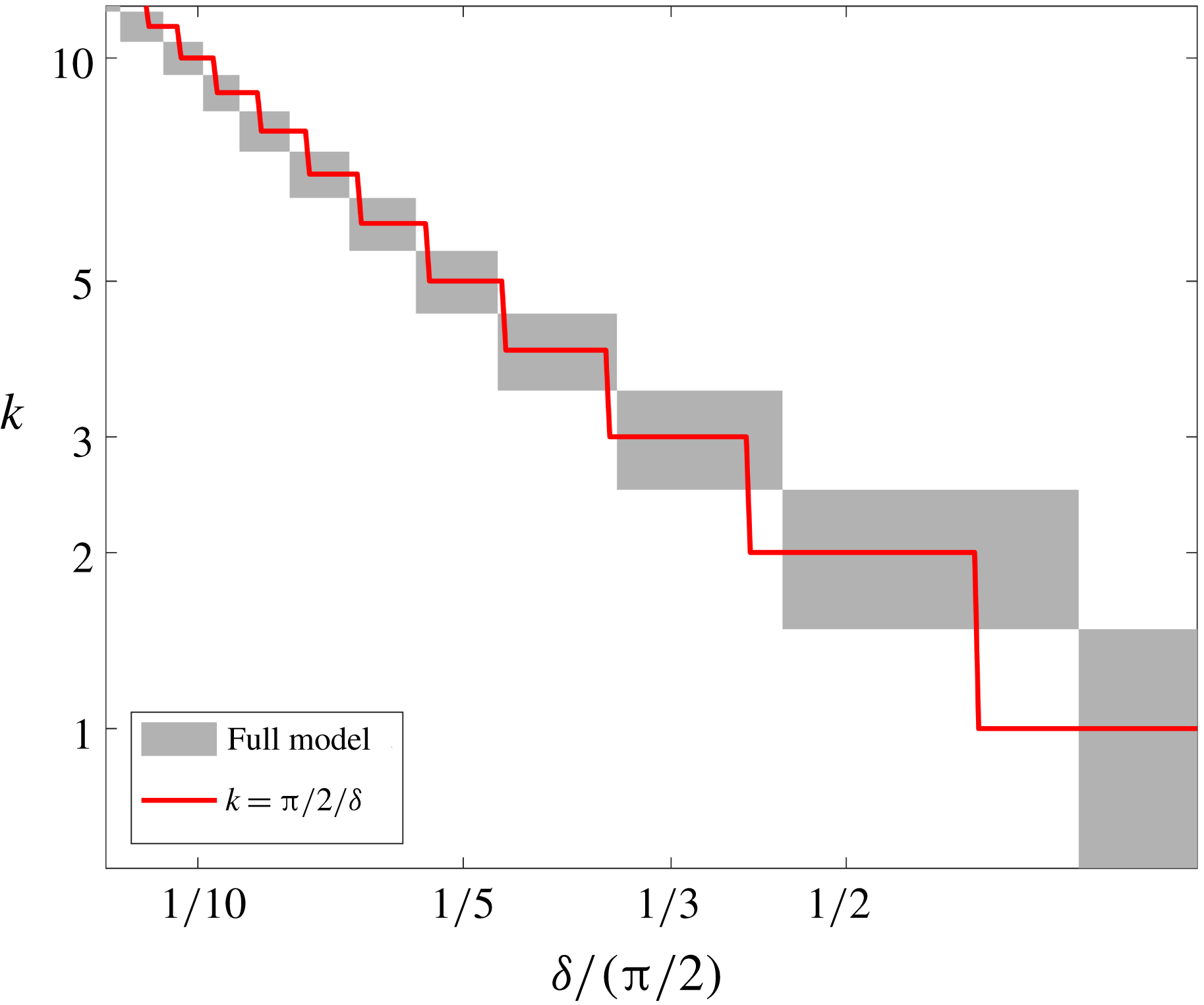
Consider now the distinguished limit
 $\unicode[STIX]{x1D6FF}\ll 1$
,
 $k\gg 1$
,
 $\unicode[STIX]{x1D6FF}k\approx 1$
and
 $n\gg 1$
, which represents the perfectly plastic limit or a fluid that is ultra-strain-rate-softening, such as paste or plasticine. Although the growth rate in this case can be derived directly by considering the limit
 $n\rightarrow \infty$
in (3.32), we choose to present the explicit model equations, as they become useful in analysing the physical mechanism in § 4. The dominant balance can be derived directly from equations (3.27) by taking the limit
 $n\rightarrow \infty$
, which leads to a thin-film model that is independent of
 $n$
 $$\begin{eqnarray}\displaystyle & \displaystyle -k^{2}u_{1}+\frac{\text{i}k}{\unicode[STIX]{x1D6FF}}v_{1}^{\prime }=\frac{p_{1}^{\prime }}{\unicode[STIX]{x1D6FF}}, & \displaystyle\end{eqnarray}$$
 $$\begin{eqnarray}\displaystyle & \displaystyle \frac{\text{i}k}{\unicode[STIX]{x1D6FF}}u_{1}^{\prime }+\frac{1}{\unicode[STIX]{x1D6FF}^{2}}v_{1}^{\prime \prime }=\text{i}kp_{1}, & \displaystyle\end{eqnarray}$$
 $$\begin{eqnarray}\displaystyle & \displaystyle \frac{1}{\unicode[STIX]{x1D6FF}}u_{1}^{\prime }+\text{i}kv_{1}=0, & \displaystyle\end{eqnarray}$$
with the boundary conditions
 $$\begin{eqnarray}u_{1}(0)=0,\quad v_{1}(0)=0,\quad \text{i}k\unicode[STIX]{x1D6FF}u_{1}(1)+v_{1}^{\prime }(1)=4\text{i}\unicode[STIX]{x1D6FF}k,\quad p_{1}(1)=0.\end{eqnarray}$$
As before, equations (3.34a–c ) can be combined into a single ordinary differential equation (ODE)
 $$\begin{eqnarray}u_{1}^{iv}+2K^{2}u_{1}^{\prime \prime }+K^{4}u_{1}=0,\end{eqnarray}$$
and the growth rate in this distinguished limit is
 $$\begin{eqnarray}\displaystyle {\mathcal{G}}_{n\rightarrow \infty }=-\cos (2K) & & \displaystyle\end{eqnarray}$$
to leading order. This implies that the unstable wavenumbers are in the range
 $$\begin{eqnarray}\frac{1}{4}\frac{\unicode[STIX]{x03C0}}{\unicode[STIX]{x1D6FF}}\leqslant k_{n\rightarrow \infty }\leqslant \frac{3}{4}\frac{\unicode[STIX]{x03C0}}{\unicode[STIX]{x1D6FF}}\end{eqnarray}$$
and that the maximum growth rate occurs for
 $2K=\unicode[STIX]{x03C0}$
, which corresponds to a most unstable wavenumber
 $k$
given by
 $$\begin{eqnarray}k\equiv \frac{\unicode[STIX]{x03C0}/2}{\unicode[STIX]{x1D6FF}}=\frac{\unicode[STIX]{x03C0}/2}{R_{0}-1}.\end{eqnarray}$$
This distinguished limit turns out to be quite useful in predicting the most unstable wavenumber also for finite
 $n$
, as implied from the thin-film solution for finite
 $n$
(figure 10
b). Moreover, (3.38) provides a reasonable prediction for the most unstable wavenumber even for large
 $\unicode[STIX]{x1D6FF}$
, as implied from a comparison with the solution to the full perturbation model at low value of
 $n$
(figure 11).
There is a special feature of the perfect plastic limit given by equation (3.36), which is that an infinite sequence of harmonics
 $K=(j+1/2)\unicode[STIX]{x03C0}$
,
 $j\in Z$
shares the maximum growth rate. This allows for the growth of linear, non-sinusoidal disturbances albeit of an identifiable fundamental wavelength.
The growth rate at the thin-film approximation and the limit
 $n\ll 1$
(- - -) compared with the complete thin-film solution (——), for
 $n$
ranging between
 $1/100$
and
 $9/10$
.

3.5.3 The distinguished limit
$\unicode[STIX]{x1D6FF}\ll 1$
,
$k\gg 1,\unicode[STIX]{x1D6FF}k\approx 1,n\ll 1$


Still in the distinguished limit in which
 $\unicode[STIX]{x1D6FF}\ll 1$
,
 $k\gg 1$
while
 $\unicode[STIX]{x1D6FF}k\approx 1$
, we now consider the case
 $n\ll 1$
where the fluid is ultra-strain-rate-hardening. In this limit we can use equations (3.27) to find that the leading-order terms are
 $$\begin{eqnarray}\displaystyle & \displaystyle \frac{2u_{1}^{\prime \prime }}{n\unicode[STIX]{x1D6FF}^{2}}-k^{2}u_{1}=\frac{p_{1}^{\prime }}{\unicode[STIX]{x1D6FF}}, & \displaystyle\end{eqnarray}$$
 $$\begin{eqnarray}\displaystyle & \displaystyle -\frac{2k^{2}}{n}v_{1}+\frac{v_{1}^{\prime \prime }}{\unicode[STIX]{x1D6FF}^{2}}=\text{i}kp_{1}, & \displaystyle\end{eqnarray}$$
 $$\begin{eqnarray}\displaystyle & \displaystyle \frac{1}{\unicode[STIX]{x1D6FF}}u_{1}^{\prime }+\text{i}kv_{1}=0 & \displaystyle\end{eqnarray}$$
 $$\begin{eqnarray}u_{1}^{iv}-\frac{4}{n}K^{2}u_{1}^{\prime \prime }+K^{4}u_{1}=0,\end{eqnarray}$$
and we find that the growth rate in this distinguished limit is
 $$\begin{eqnarray}\displaystyle {\mathcal{G}}_{n\rightarrow 0}=-1+n\left(1-\frac{1}{\cosh \left(\displaystyle \frac{2K}{\sqrt{n}}\right)}\right) & & \displaystyle\end{eqnarray}$$
to leading order in
 $n$
, which is negative for all
 $K$
(e.g. figure 12) and is consistent with (3.32) in the limit
 $n\rightarrow 0$
.
4 Physical interpretation of the tearing mechanism
4.1 The structure of the growth rate
To reveal the physical mechanism behind the instability we now investigate the structure of the growth rate (3.14) by deriving a more explicit expression for the radial perturbation velocity at the front,
 $u_{1}(R_{0})$
. Combining the boundary condition of no-tangential and no-normal stresses (3.15b
), the perturbation shear stress at the base-state front is
 $$\begin{eqnarray}\unicode[STIX]{x1D70E}_{1r\unicode[STIX]{x1D703}}(R_{0})=\frac{1}{R_{0}}\frac{\unicode[STIX]{x2202}R_{1}}{\unicode[STIX]{x2202}\unicode[STIX]{x1D703}}\unicode[STIX]{x1D70E}_{0\unicode[STIX]{x1D703}\unicode[STIX]{x1D703}}(R_{0}).\end{eqnarray}$$
By taking a derivative with respect to
 $\unicode[STIX]{x1D703}$
,
 $$\begin{eqnarray}\frac{\unicode[STIX]{x2202}\unicode[STIX]{x1D70E}_{1r\unicode[STIX]{x1D703}}}{\unicode[STIX]{x2202}\unicode[STIX]{x1D703}}(R_{0})=\frac{1}{R_{0}}\frac{\unicode[STIX]{x2202}^{2}R_{1}}{\unicode[STIX]{x2202}\unicode[STIX]{x1D703}^{2}}\unicode[STIX]{x1D70E}_{0\unicode[STIX]{x1D703}\unicode[STIX]{x1D703}}(R_{0}),\end{eqnarray}$$
we see that the left-hand side is a radial force. Substituting the definition of the shear stress in terms of the perturbation velocities (3.6c ) leads to
 $$\begin{eqnarray}\unicode[STIX]{x1D707}_{0}\frac{\unicode[STIX]{x2202}}{\unicode[STIX]{x2202}\unicode[STIX]{x1D703}}\left[\frac{1}{r}\frac{\unicode[STIX]{x2202}u_{1}}{\unicode[STIX]{x2202}\unicode[STIX]{x1D703}}+r\frac{\unicode[STIX]{x2202}}{\unicode[STIX]{x2202}r}\left(\frac{v_{1}}{r}\right)\right]=\frac{1}{R_{0}}\frac{\unicode[STIX]{x2202}^{2}R_{1}}{\unicode[STIX]{x2202}\unicode[STIX]{x1D703}^{2}}\unicode[STIX]{x1D70E}_{0\unicode[STIX]{x1D703}\unicode[STIX]{x1D703}},\end{eqnarray}$$
and solving for
 $u_{1}$
we find that
 $$\begin{eqnarray}u_{1}=\frac{\unicode[STIX]{x1D70E}_{0\unicode[STIX]{x1D703}\unicode[STIX]{x1D703}}}{\unicode[STIX]{x1D707}_{0}}R_{1}+\frac{R_{0}^{2}}{k^{2}}\frac{\unicode[STIX]{x2202}}{\unicode[STIX]{x2202}r}\left(\frac{1}{r}\frac{\unicode[STIX]{x2202}v_{1}}{\unicode[STIX]{x2202}\unicode[STIX]{x1D703}}\right).\end{eqnarray}$$
Substituting this in the growth rate (3.14) results in
 $$\begin{eqnarray}{\mathcal{G}}(k,n,R_{0})=-\frac{1}{R_{0}^{2}}+\frac{\unicode[STIX]{x1D70E}_{0\unicode[STIX]{x1D703}\unicode[STIX]{x1D703}}}{\unicode[STIX]{x1D707}_{0}}+\frac{R_{0}^{2}}{k^{2}R_{1}}\frac{\unicode[STIX]{x2202}}{\unicode[STIX]{x2202}r}\left(\frac{1}{r}\frac{\unicode[STIX]{x2202}v_{1}}{\unicode[STIX]{x2202}\unicode[STIX]{x1D703}}\right),\end{eqnarray}$$
where the three contributions to
 ${\mathcal{G}}$
represent the geometric stretching, hoop stress and momentum dissipation. In the thin-film limit (
 $\unicode[STIX]{x2202}/\unicode[STIX]{x2202}r\gg 1/r$
)
 $R_{0}\sim 1$
and the growth rate simplifies to
 $$\begin{eqnarray}{\mathcal{G}}(K,n)=-1+4-\frac{u_{1}^{\prime \prime }}{K^{2}R_{1}},\end{eqnarray}$$
where the three contributions correspond to those in (4.5a ), and where mass continuity at the same limit was used to present the dissipation contribution in terms of the radial velocity.
4.2 Geometric stretching
The circular geometry of the flow combined with mass continuity implies that the extensional strain rates of the base flow are
 $e_{0rr}=\unicode[STIX]{x2202}u_{0}/\unicode[STIX]{x2202}r=-1/R_{0}^{2}$
and
 $e_{0\unicode[STIX]{x1D703}\unicode[STIX]{x1D703}}=u_{0}/r=1/R_{0}^{2}$
. Therefore, as the fluid front advances in a circular geometry it stretches azimuthally and slows down radially. This geometrical stretching, which is independent of
 $n$
and
 $k$
, gives rise to the first stabilising term in the growth rate (4.5).
(a) The leading front of the base state (

 $\hat{\unicode[STIX]{x1D703}}\hat{\unicode[STIX]{x1D703}}$
direction, while the other stress components are zero. (b) The base-state normal stress contributes to tangential stress at the perturbed interface (

 $\hat{r}\hat{\unicode[STIX]{x1D703}}$
direction of the base front that is proportional to the slope of the perturbed front. (c) The secondary flow following a geometric perturbation (
 $\downarrow$
green colour) consists of two distinct patterns through which momentum dissipates and stabilises the perturbation. At
 $K\lesssim \unicode[STIX]{x03C0}/2$
, the streamlines stretch circumferentially from frontal depressions to frontal bulges through a relatively long path along which energy is dissipated. At
 $K\gtrsim \unicode[STIX]{x03C0}/2$
, vortices form near the inner boundary and screen the interior from the front, so that less fluid is available to sustain the growth of tongues. The volume covered with vortices grows with
 $K$
.

The base-flow tension at the leading front is represented by the hoop stress as a function of the fluid exponent.

4.3 Instability
The flow in the base state is axisymmetric and diminishes towards the moving front (figure 13
a), having radially growing viscosity (
 $n>1$
), declining viscosity (
 $n<1$
) or uniform viscosity (
 $n=1$
). The extensional stress in the
 $\hat{\unicode[STIX]{x1D703}}\hat{\unicode[STIX]{x1D703}}$
direction (hoop stress) at the base-flow front
 $$\begin{eqnarray}\unicode[STIX]{x1D70E}_{0\unicode[STIX]{x1D703}\unicode[STIX]{x1D703}}(R_{0})=-p_{0}+2\unicode[STIX]{x1D707}_{0}e_{0\unicode[STIX]{x1D703}\unicode[STIX]{x1D703}}=4R_{0}^{-2/n}\end{eqnarray}$$
is always positive (3.4c
), implying that the fluid front is under tension throughout the evolution. Although the tension grows larger the smaller
 $R_{0}>1$
is and the more strain-rate softening (
 $n>1$
) the fluid is (figure 14), its contribution to the growth rate (4.5a
) is the constant
 $\unicode[STIX]{x1D70E}_{0\unicode[STIX]{x1D703}\unicode[STIX]{x1D703}}/\unicode[STIX]{x1D707}_{0}=4R_{0}^{-2}$
namely, destabilising and independent of
 $k$
and
 $n$
. The instability develops due to the interaction of the base-flow hoop stress with the geometric perturbation: the geometric perturbation of the front forms forward bulges and depressions along the front (figure 13
b). Consequently, the base-flow hoop stress at the front has a non-zero contribution to the tangential stress along the perturbed interface. Since the total tangential stress along the front must be zero, the perturbation field has a non-zero shear stress along the base-state interface that balances the contribution of the coupled hoop stress and geometric perturbation (4.1). That is, the interfacial curvature leads to a base-flow hoop stress that leads to a perturbation shear stress due to the perturbed interface. The perturbation shear stress, which is proportional to the slope of the perturbed interface
 $\unicode[STIX]{x1D70E}_{1r\unicode[STIX]{x1D703}}(R_{0})\propto \unicode[STIX]{x2202}R_{1}/\unicode[STIX]{x2202}\unicode[STIX]{x1D703}$
(4.1) forces a secondary flow along the base-flow front to converge into forward bulges in the perturbed interface and diverge from interfacial troughs, independently of the fluid exponent
 $n$
. Consequently, the secondary flow transports fluid from interfacial troughs to bulges, enhancing the perturbation growth. The development of the instability leads to the relaxation of hoop stresses within the growing fingers, so that no additional fingers form at the edges of existing fingers, as experimental evidence indicates (see Sayag & Worster Reference Sayag and Worster2019).
We note that with a planar interface in a two-dimensional geometry, hoop stresses, or extensional stresses transverse to the flow are absent. Therefore, the circular geometry is crucial in generating a base-flow hoop stress, which is the source of the instability.
Another way to think of the instability is in terms of forces. In the thin-film base state, the radial extensional force
 $\unicode[STIX]{x2202}\unicode[STIX]{x1D70E}_{0rr}/\unicode[STIX]{x2202}r$
is positive along a radius (3.4b
), though it is smaller at the leading front than in the interior due to the base-state hoop stress that stretches the fluid azimuthally. Following a perturbation, the contribution to the extensional force
 $\unicode[STIX]{x2202}\unicode[STIX]{x1D70E}_{1rr}/\unicode[STIX]{x2202}r$
is equivalent, in the thin-film limit, to
 $-\unicode[STIX]{x2202}\unicode[STIX]{x1D70E}_{1r\unicode[STIX]{x1D703}}/\unicode[STIX]{x2202}\unicode[STIX]{x1D703}$
, which equals at the leading front to
 $k^{2}/R_{0}\unicode[STIX]{x1D70E}_{0\unicode[STIX]{x1D703}\unicode[STIX]{x1D703}}(R_{0})R_{1}$
(4.2). Therefore, the total extensional force at the front grows along a bulge (
 $R_{1}>0$
) and diminishes along a trough (
 $R_{1}<0$
), resulting in a greater radial force along a forward bulge.
4.4 Stability and the impact of the fluid exponent
$n$

The contribution of momentum dissipation to the growth rate (4.5a ) is also stabilising, but unlike the uniform stabilisation of geometric stretching (§ 4.2), it depends on both the wavenumber and the fluid exponent. In particular, the mechanism of momentum dissipation is qualitatively different between low and high wavenumbers. To see this we use the growth rate in the thin-film limit (4.5b ), which has the closed-form solution given by (3.32).
4.4.1 Long-wavelength limit: lateral flow
Expanding (3.32) assuming
 $K\ll 1$
we find that
 $$\begin{eqnarray}{\mathcal{G}}_{K\ll 1}\approx -1+2K^{2}\end{eqnarray}$$
to leading order in
 $K$
, which tends to
 $-1$
in the
 $K\rightarrow 0$
limit. This implies that stability in the small-wavenumber
 $K$
limit (
 $K\ll \unicode[STIX]{x03C0}/2$
) is independent of the fluid exponent
 $n$
to leading order (figure 15). Since
 $K=k\unicode[STIX]{x1D6FF}$
, this limit corresponds to either small wavenumbers
 $k$
and thus long wavelengths, or to extremely thin films. Stability in this long-wavelength limit may result from the relatively long circumferential and open streamlines in the secondary flow, along which the total dissipation of momentum is substantial (figure 13
c). As the wavelength turns shorter (wavenumber larger) the streamlines get shorter so less momentum dissipates, whereas the destabilising hoop stress remains unchanged, which allows the instability to grow.
The growth rate in the thin-film limit (solid lines) as a function of the effective wavenumber
 $K$
for fluid exponents
 $n=0.5,1,5$
(colour). The asymptotic behaviour of the growth rate in the small-wavenumber limit
 $(K\ll 1)$
is independent of
 $n$
to leading order (dash line). In the large-wavenumber limit
 $(K\gg 1)$
the growth rate has a leading-order dependence on the fluid exponent (dash–dot).

4.4.2 Short-wavelength limit: vortices
In the large wavenumber
 $K$
limit, the growth rate (3.32) has the simplified form
 $$\begin{eqnarray}{\mathcal{G}}_{K\gg 1}\approx -1+2K^{2}\left(\frac{\text{sin}(K\sqrt{(n-1)/n})}{K\sqrt{(n-1)/n}\cosh (K/\sqrt{n})}\right)^{2},\end{eqnarray}$$
which implies that stability in large wavenumbers (
 $K\gg \unicode[STIX]{x03C0}/2$
) depends also on the fluid exponent
 $n$
to leading order (figure 15). This limit corresponds to either large wavenumbers
 $k$
and thus short wavelengths, or to relatively thicker films. In this short-wavelength limit, we expect dissipation to be enhanced due to the corresponding large gradients. This is naturally the case for a Newtonian fluid due to the constant viscosity. However, for
 $n\neq 1$
the growth of dissipation with the wavenumber is not straightforward since the strain-rate-dependent viscosity also changes. Specifically, the viscosity varies with both the wavenumber and
 $n$
as implied from equation (3.9) and figure 6. In fact, in the
 $K\gg 1$
limit the dissipation dominates and is a weak function of
 $n$
such that
 ${\mathcal{G}}\rightarrow -1$
in the
 $K\rightarrow \infty$
limit. The sensitivity to
 $n$
grows at intermediate wavenumbers (
 $K\approx \unicode[STIX]{x03C0}/2$
), in which the dissipation is stronger than the Newtonian case when
 $n<1$
and weaker when
 $n>1$
(figure 15), thereby allowing the instability for strain-rate-softening fluids.
The exact perturbation vorticity
 $\unicode[STIX]{x1D714}_{1}/k$
(colour) and streamlines (vortices are clockwise


 $K=1.5,1.75,2$
(
 $\unicode[STIX]{x1D6FF}=0.25;k=6,7,8$
), and for (columns)
 $n=0.3,1,3$
. The volume covered with vortices grows the larger
 $K$
is and the smaller
 $n$
is, and the corresponding growth rate declines. Streamlines absolute values:
 $0.001,0.002,0.004,0.008,0.016,0.032,0.064,0.128,0.256,0.512$
.

Another important consequence of the shortwave limit is the emergence of vortices (closed streamlines) in the secondary flow, which form near the inner boundary and are centred at the boundaries between interfacial depressions and bulges (figure 13
c). Since the mass flux out of a vortex is zero, the fluid that contributes to the growth of perturbation comes from the region without vortices, which gets smaller with
 $K$
and/or as
 $n$
declines (figure 16). That is, vortices screen the front from the fluid interior, so that there is no secondary-flow mass flux from the vortex region to the front region. Consequently, with the growth of the vortex-covered area with
 $K$
the radial velocity at the front declines and so does the growth rate.
A measure of the behaviour of the secondary-flow vortices can be provided by the perturbation vorticity
 $$\begin{eqnarray}\displaystyle \unicode[STIX]{x1D714}_{1}\equiv (\unicode[STIX]{x1D735}\times \boldsymbol{u}_{1})\boldsymbol{\cdot }\hat{\boldsymbol{z}}=\frac{\unicode[STIX]{x2202}v_{1}}{\unicode[STIX]{x2202}r}+\frac{v_{1}}{r}-\frac{1}{r}\frac{\unicode[STIX]{x2202}u_{1}}{\unicode[STIX]{x2202}\unicode[STIX]{x1D703}}, & & \displaystyle\end{eqnarray}$$
which simplifies in the thin-film limit (
 $\unicode[STIX]{x1D6FF}\ll 1$
) to
 $$\begin{eqnarray}\displaystyle \unicode[STIX]{x1D714}_{1}\approx \frac{1}{\unicode[STIX]{x1D6FF}}\frac{\unicode[STIX]{x2202}v_{1}}{\unicode[STIX]{x2202}\unicode[STIX]{x1D709}}-\frac{\unicode[STIX]{x2202}u_{1}}{\unicode[STIX]{x2202}\unicode[STIX]{x1D703}}, & & \displaystyle\end{eqnarray}$$
to leading order. Considering first the case
 $n\gg 1$
(§ 3.5.2), which corresponds to the largest growth rates for all
 $K$
, the vorticity to leading order in
 $\unicode[STIX]{x1D6FF}$
 $$\begin{eqnarray}\unicode[STIX]{x1D714}_{1}=2\frac{\unicode[STIX]{x2202}R_{1}}{\unicode[STIX]{x2202}\unicode[STIX]{x1D703}}[2K\unicode[STIX]{x1D709}\sin (K(1-\unicode[STIX]{x1D709}))+\cos (K(1+\unicode[STIX]{x1D709}))+\cos (K(1-\unicode[STIX]{x1D709}))]\end{eqnarray}$$
has harmonic structure along a radius. Specifically, the signature of
 $\unicode[STIX]{x1D714}$
changes along a radius at a growing frequency with
 $K$
. This implies that the secondary flow along a radius consists of coexisting clockwise and counterclockwise vortices, whose number grows with
 $K$
(figure 17), or equivalently with both
 $k$
and
 $\unicode[STIX]{x1D6FF}$
. This oscillatory structure is slightly reminiscent of flows of strain-rate-softening fluid around a contracting cavity (Dallaston & Hewitt Reference Dallaston and Hewitt2014), though with some qualitative differences. Along the boundaries
 $\unicode[STIX]{x1D709}=0,1$
, the perturbation vorticity is
 $$\begin{eqnarray}\displaystyle & \displaystyle \unicode[STIX]{x1D714}_{1}(1)=4\frac{\unicode[STIX]{x2202}R_{1}}{\unicode[STIX]{x2202}\unicode[STIX]{x1D703}}\cos ^{2}(K), & \displaystyle\end{eqnarray}$$
 $$\begin{eqnarray}\displaystyle & \displaystyle \unicode[STIX]{x1D714}_{1}(0)=4\frac{\unicode[STIX]{x2202}R_{1}}{\unicode[STIX]{x2202}\unicode[STIX]{x1D703}}\cos (K), & \displaystyle\end{eqnarray}$$
 $\unicode[STIX]{x1D709}=1$
) follows the sign of the interface slope and is independent of
 $K$
. However, near the inner boundary (
 $\unicode[STIX]{x1D709}=0$
) the rotation direction of the vortices changes with both the slope of the leading front and with
 $K$
. This implies that new vortices emerge at the inner boundary as
 $K$
grows, and that existing vortices are displaced radially towards the leading front (see movie available at https://doi.org/10.1017/jfm.2019.778). The azimuthal size of these vortices is half the azimuthal wavelength
 $\unicode[STIX]{x03C0}\unicode[STIX]{x1D6FF}/K$
, which is equivalent to the radial size (half the radial wavelength), as implied by (4.10). Therefore, the number of vortices along an annulus of thickness
 $\unicode[STIX]{x1D6FF}$
grows like
 $K/\unicode[STIX]{x03C0}$
, forming a vortex street that covers the whole flow domain (figure 18
b).
The normalised vorticity
 $\unicode[STIX]{x1D714}/ki$
in the limit
 $n\gg 1$
(4.10) along a radius, for several values of
 $K=1.5,3,6$
.
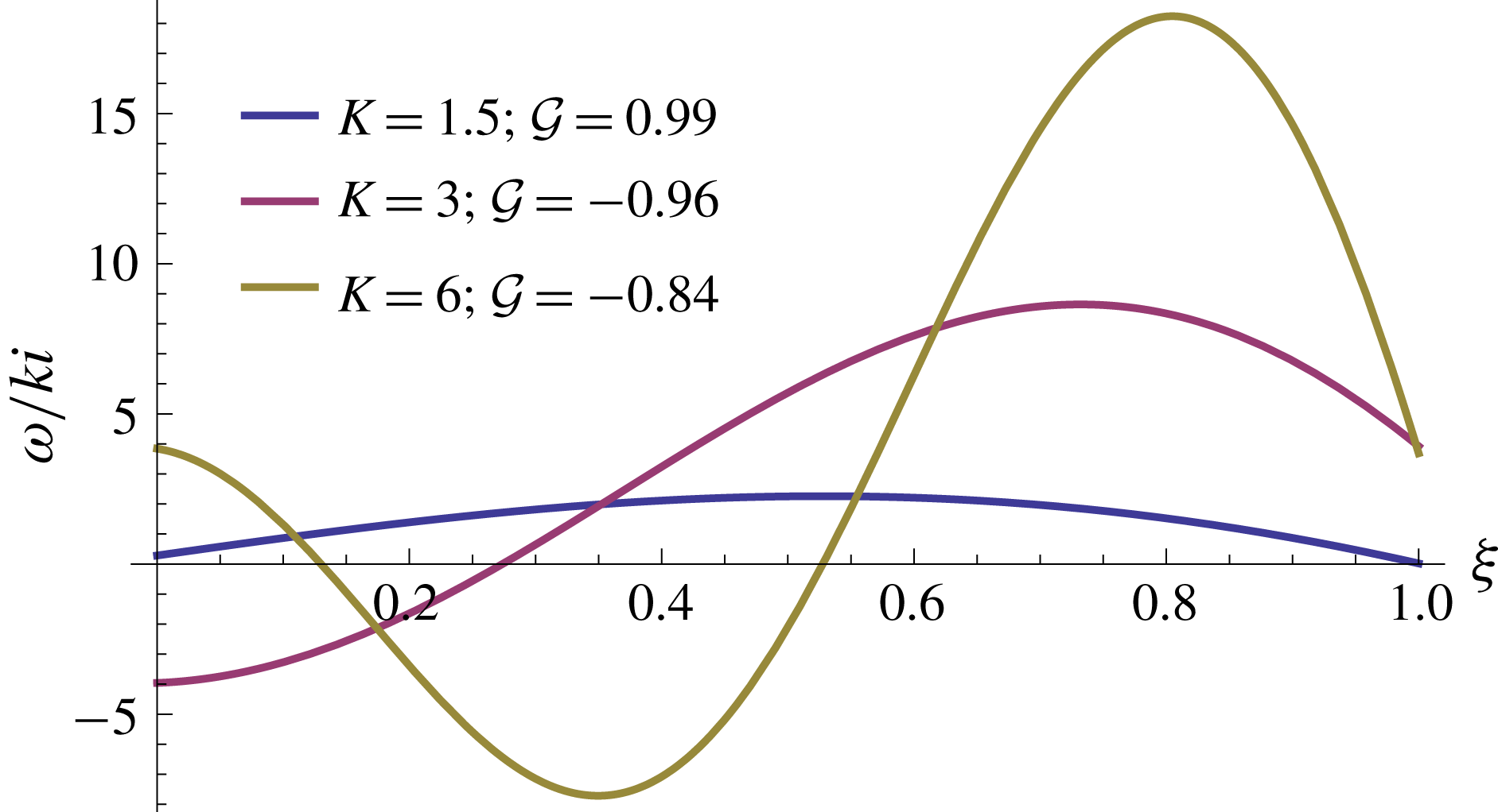
When
 $n\leqslant 1$
(strain-rate thickening), the solution for the radial velocity (3.30) is no longer harmonic because
 $b$
is imaginary (3.31). Therefore, the vorticity is also non-harmonic and the domain of radial size
 $\unicode[STIX]{x1D6FF}$
can only contain a single vortex (figure 18
a).
Vorticity and vortex street: the exact perturbation vorticity
 $\unicode[STIX]{x1D714}_{1}/k$
(colour) and streamlines (vortices are clockwise


 $K=30$
(
 $\unicode[STIX]{x1D6FF}=0.75;k=40$
) and for (a)
 $n=1$
(streamlines absolute value:
 $0.5,0.1,10^{-2},10^{-3},10^{-4},10^{-5},10^{-6},10^{-7},10^{-8}$
), and (b)
 $n=100$
(streamlines absolute values:
 $0.75,0.5,0.25,0.05$
).

4.5 Contrast with classical fingering instability
It is insightful to contrast the present mechanism with the classical viscous-fingering instability. Considering a shear-dominated flow of Newtonian fluid of viscosity
 $\unicode[STIX]{x1D707}_{d}$
displacing at constant flux
 $Q$
an ambient Newtonian fluid of viscosity
 $\unicode[STIX]{x1D707}_{a}$
inside a Hele-Shaw cell of uniform gap
 $h$
in polar coordinates, the growth rate is (Paterson Reference Paterson1981)
 $$\begin{eqnarray}{\mathcal{G}}_{Paterson}=\frac{Q/h}{2\unicode[STIX]{x03C0}r_{0}^{2}}\left[-1+k\frac{\unicode[STIX]{x1D707}_{a}-\unicode[STIX]{x1D707}_{d}}{\unicode[STIX]{x1D707}_{a}+\unicode[STIX]{x1D707}_{d}}\right]-\unicode[STIX]{x1D70E}\frac{k(k^{2}-1)}{r_{0}^{3}}\frac{\unicode[STIX]{x1D707}_{a}\unicode[STIX]{x1D707}_{d}}{\unicode[STIX]{x1D707}_{a}+\unicode[STIX]{x1D707}_{d}},\end{eqnarray}$$
where
 $r_{0}(t)$
is the radius of the base-state interface when the perturbation is applied. Surface tension
 $\unicode[STIX]{x1D70E}$
at the fluid–fluid interface is stabilising for all wavenumbers and fluid viscosities. Therefore, for all wavenumbers instability can occur only if the viscosity of the displacing fluid is smaller (
 $\unicode[STIX]{x1D707}_{d}<\unicode[STIX]{x1D707}_{a}$
). Particularly, in the absence of surface tension and if the viscosity of the displaced fluid is negligible (
 $\unicode[STIX]{x1D707}_{a}\ll \unicode[STIX]{x1D707}_{d}$
), as in the flow that we study, the shear-dominated growth rate simplifies to
 $$\begin{eqnarray}{\mathcal{G}}_{Paterson}|_{\unicode[STIX]{x1D70E}=0,\unicode[STIX]{x1D707}_{a}\ll \unicode[STIX]{x1D707}_{d}}=\frac{Q/h}{2\unicode[STIX]{x03C0}r_{0}^{2}}(-1-k).\end{eqnarray}$$
In contrast, the flow that we consider in this paper is extensionally dominated and the displacing fluid has a strain-rate-dependent viscosity. The resulting dimensional growth rate in the thin-film limit (
 $\unicode[STIX]{x1D6FF}\ll 1$
)
 $$\begin{eqnarray}\displaystyle {\mathcal{G}}=\frac{Q/h}{2\unicode[STIX]{x03C0}r_{0}^{2}}\left[-1+\frac{2n\sin ^{2}\left(K\sqrt{\displaystyle \frac{n-1}{n}}\right)}{\sin ^{2}\left(K\sqrt{\displaystyle \frac{n-1}{n}}\right)+(n-1)\cosh ^{2}\left(\displaystyle \frac{K}{\sqrt{n}}\right)}\right] & & \displaystyle\end{eqnarray}$$
implies that if the fluid is strain-rate softening (
 $n>1$
), the interface is unstable for some wavenumbers
 $K=k\unicode[STIX]{x1D6FF}$
. Such an unstable configuration corresponds to a highly viscous fluid displacing an low-viscosity ambient fluid, a configuration that remains stable in the classical shear-dominated fingering case.
5 Consistency with experimental evidence
The theory we have developed here is aimed at explaining the spatio-temporal patterns that were discovered in a series of laboratory experiments with strain-rate-softening polymer solutions in Part 1 (Sayag & Worster Reference Sayag and Worster2019). One important result of these experiments is that the fingered interfaces coarsened over time: as the front of the displacing fluid evolved, the number of floating tongues declined through the progressive closure of some of the tears that separated them, resulting in the merging of adjacent tongues into wider ones. This coarsening or cascade of the dominant wavenumbers, either converged in time to a lower integer wavenumber, or kept alternating, apparently stochastically, within a range of lower wavenumbers. The results of these experiments were combined into a single graph that shows the evolution of the dominant wavenumbers for the different source flux used (figure 9b, Sayag & Worster Reference Sayag and Worster2019), in which time was non-dimensionalised with the characteristic scale
 ${\mathcal{T}}=2\unicode[STIX]{x03C0}hr_{G}^{2}/Q$
that is also used in the theoretical part (2.6).
The wavenumber cascade mechanism that we observed experimentally in Part 1 (Sayag & Worster Reference Sayag and Worster2019) was operating also when the propagating front was far from the initial circular state, which suggests that it is primarily a nonlinear process. Therefore, there is no apparent reason to expect that the present linear-stability analysis can predict such late-time evolution in the experiments that departs from a circular base state by far. And yet, our theoretical results in the present part also involve a wavenumber cascade. Specifically, for a fixed
 $n$
in the full linear theory the most unstable wavenumber declines monotonically with
 $\unicode[STIX]{x1D6FF}$
. This implies that an unstable front will develop more fingers the earlier the perturbation is made, while fewer fingers will emerge following a perturbation at later times (figure 5
a). Therefore, we evaluate the instantaneous most unstable wavenumbers as a function of the base-state thickness
 $\unicode[STIX]{x1D6FF}$
, as in figure 11 but replacing
 $\unicode[STIX]{x1D6FF}(t)$
with the explicit dependence on time (3.3), and consider this as a time evolution of the dominant wavenumber. We find that this interpretation of the dependence of the most unstable wavenumber on the base-state thickness
 $\unicode[STIX]{x1D6FF}(t)$
provides a consistent prediction to the initial cascading evolution of the measured dominant wavenumbers (figure 19). Furthermore, the prediction of the perfectly plastic, thin-film model for the most unstable wavenumber (3.38) that is written explicitly in terms of time
 $$\begin{eqnarray}k_{max}=\frac{\unicode[STIX]{x03C0}}{2}\left[-1+\sqrt{\frac{Q}{\unicode[STIX]{x03C0}hr_{G}^{2}}t+1}\right]^{-1}\end{eqnarray}$$
also provides a surprisingly consistent prediction for the experimental evolution of the dominant wavenumbers (figure 19).
Comparison of the predicted most-unstable modes and the time evolution of the dominant wavenumbers measured in laboratory experiments for
 $n=6$
(Sayag & Worster Reference Sayag and Worster2019). The experimental measurements (colour) represent the dominant Fourier modes that the front is comprised of at each instant for a range of source fluxes
 $0.7\lesssim Q\lesssim 13.4~\text{g}~\text{s}^{-1}$
. Also shown are the corresponding instantaneous most-unstable modes predicted by the full perturbation model (

 $n\gg 1$
) thin-film model (5.1) (


The apparent correspondence between the linear-theory prediction and the cascading phase of the experimental observations is surprising. It implies that at any instant the dominant wavenumber of an experimental pattern, which can be far from a circular shape, is equivalent to the most unstable wavenumber of a perturbed circular state that has the same volume. This appears to suggest that the wavenumber the system settles on is determined to leading order by the total discharged volume, and that other interactions may be secondary.
Our experimental observations suggest that throughout their evolution there was no apparent flow within the tongues, and that they were displaced as solid objects. The most active flow in the free-slip domain (
 $r>r_{G}$
) seemed to concentrate within a thin region of width
 ${\approx}h$
near
 $r_{G}$
. This may imply that the finite-time evolution of the patterns is determined by the flow in the vicinity of
 $r_{G}$
and that the tongues are passive components. The interpretation of our theoretical results predicts that the cascade of wavenumbers ends at
 $k=1$
. Such a situation was not observed experimentally, apart from some experimental indications of a trend toward a
 $k=1$
mode at the high-end flux regime (Sayag & Worster Reference Sayag and Worster2019).
The transition at low
 $Q$
to a stochastic late-time evolution, which we identified experimentally (figure 19
c,d) is not captured by the theoretical model. This could be simply a consequence of late-time evolution that our linear model cannot resolve. It could also be a result of the relatively simple constitutive model that we used. For example, accounting for a low strain-rate behaviour such as bounded viscosity should introduce another time scale, which may lead to the differentiation between a regular and stochastic evolution with respect to
 $Q$
. The interaction with the flow of the ambient fluid within the tears may also have an effect, though we do not account for it at present.
6 Conclusions
Inspired by the experimental study in Part 1 (Sayag & Worster Reference Sayag and Worster2019), we developed a model to investigate the development of the observed tear-like patterns and their coarsening in time. Our theoretical model includes three elements that we believe are critical to the appearance of the instability: the free-slip conditions along the base and the surface boundaries of the displacing fluid; the circular geometry that imposes circumferential tension along the leading front; and the nonlinear deformation law of the displacing fluid. We found that axisymmetric solutions can become linearly unstable, having a most unstable wavenumber that is inversely proportional to the thickness of the base state
 $\unicode[STIX]{x1D6FF}(t)$
, to leading order. Consequently, the thicker the base-flow annular layer is, the smaller the number of tears that would evolve. The mechanism of the instability appears fundamentally different from that of the classical viscous fingering: the source of the instability is the base-flow hoop stress along the leading front. The projection of that stress over the perturbed interfacial geometry results in a perturbation shear stress along the base-flow front that varies azimuthally with the shape of the perturbed front. Such shear-stress distribution results in circumferential flow along the interface that converges into forward bulges and diverges from troughs in the perturbed interface and thus sustains the perturbation growth. We emphasise that the destabilising hoop stress is independent of the wavenumber and of the nonlinearity of the fluid. Rather, the base-flow hoop stress is a consequence of the flow geometry and it is present for all fluid exponents and particularly for both Newtonian and strain-rate-softening fluids. In contrast, the momentum dissipation associated with shear suppresses the perturbations through two different mechanisms at low and high wavenumbers. At the lower-end wavenumbers the secondary flow consists of open circumferential streamlines along which fluid is carried from perturbation depressions to perturbation bulges on a relatively long dissipative path. At the higher-end wavenumbers the dissipation is modified by larger velocity gradients, and the secondary flow consists of vortices that screen perturbation flow from the leading front. The combined impact of these stabilising mechanisms is weakest at wavenumbers
 ${\sim}1/\unicode[STIX]{x1D6FF}$
and the more strain-rate softening the fluid is. This defines the wavenumbers that grow fastest and that dominate the front pattern.
We find that our fluid-mechanical approach to explain a phenomenon that involves tear-like patterns leads to predictions that are consistent with some major characteristics of the experimental measurements of Part 1, including the inverse cascade of the dominant wavenumber, which is predominantly a nonlinear process. Our theoretical model relates to power-law fluids and neglects other potential non-Newtonian properties. The fact that the model includes a single dimensionless number
 $n$
, associated with the way the fluid viscosity responds to strain rate, implies that the patterns that we observed in polymer solutions may be dynamically similar to other strain-rate-softening fluids under circular extension in inertia-free flow, independently of the spatio-temporal scales of the flow and independently of the material microscopic structures. Particularly, our results may apply to systems ranging from pastes squeezed in laboratory scale to polycrystalline ice creeping into the open ocean on a global scale.
Acknowledgements
R.S. thanks SIDEER and BIDR in Ben-Gurion University, Israel, for financial support, and DAMTP, University of Cambridge, UK, where some of this research had took place. This research was supported by the Israel Science Foundation (grant no. 1368/16).
Supplementary movie
Supplementary movie is available at https://doi.org/10.1017/jfm.2019.778.
Appendix A. The Newtonian-fluid limit
$n=1$

The coefficients
 $c_{1\ldots 4}$
of the solution in the Newtonian limit (3.20) are
 $$\begin{eqnarray}\displaystyle \left.\begin{array}{@{}c@{}}\displaystyle c_{1}=\frac{k(R_{0}^{2k}+k(R_{0}^{2}-1)+1)}{k^{2}R_{0}^{k+1}-2(k^{2}-1)R_{0}^{k+3}+k^{2}R_{0}^{k+5}+R_{0}^{3-k}+R_{0}^{3k+3}}R_{1},\\ \displaystyle c_{2}=\frac{k(-(k+1)R_{0}^{2k}+kR_{0}^{2k+2}-1)}{k^{2}R_{0}^{k+1}-2(k^{2}-1)R_{0}^{k+3}+k^{2}R_{0}^{k+5}+R_{0}^{3-k}+R_{0}^{3k+3}}R_{1},\\ \displaystyle c_{3}=-\frac{k(k(R_{0}^{2}-1)+R_{0}^{2}(R_{0}^{2k}+1))}{k^{2}R_{0}^{k+1}-2(k^{2}-1)R_{0}^{k+3}+k^{2}R_{0}^{k+5}+R_{0}^{3-k}+R_{0}^{3k+3}}R_{1},\\ \displaystyle c_{4}=\frac{k(kR_{0}^{2k}-(k-1)R_{0}^{2k+2}+R_{0}^{2})}{k^{2}R_{0}^{k+1}-2(k^{2}-1)R_{0}^{k+3}+k^{2}R_{0}^{k+5}+R_{0}^{3-k}+R_{0}^{3k+3}}R_{1}.\end{array}\right\} & & \displaystyle\end{eqnarray}$$



