1 Introduction
The vast majority of the literature on aerosol particle transport treats the particles as if they are isolated when calculating the drag. This approach is valid for very dilute aerosols, where the average separation between particles is large, and thus hydrodynamic interactions between particles are negligible. For example, the mean settling velocity of a system of spheres in continuum flow is
 $U_{0}(1-6.55\unicode[STIX]{x1D719})$
, where
 $\unicode[STIX]{x1D719}$
is the particle volume fraction and
 $U_{0}$
is the velocity each sphere would have if it was alone in an infinite fluid (Batchelor Reference Batchelor1972). As another example, the viscosity of a suspension of spheres in continuum flow is
 $\unicode[STIX]{x1D707}(1+2.5\unicode[STIX]{x1D719})$
, where
 $\unicode[STIX]{x1D707}$
is the fluid viscosity (Friedlander Reference Friedlander2000). Clearly, the interaction effects on the settling velocity and suspension viscosity are negligible for aerosol systems consisting of spheres at typical volume fractions.
However, there are situations where one might expect interactions between particles to be more significant. Sorensen et al. (Reference Sorensen, Hageman, Rush, Huang and Oh1998) has demonstrated that aerogels can form under certain conditions in sooting flames. In this process, fractal aggregates formed by diffusion-limited cluster aggregation (DLCA) reach a critical size and begin to fill the entire physical volume because the aggregate fractal dimension (
 $d_{f}\approx 1.78$
) is less than the spatial dimension. One would expect hydrodynamic interactions between the soot aggregates to be more significant than between spheres at the same volume fraction, due to the stringy nature of the DLCA aggregates. More generally, for coagulating systems aerosol particles must approach each other, so that interparticle hydrodynamic interactions may affect the coagulation rate.
Much of the literature on hydrodynamic interactions between particles focuses on spheres in the continuum regime (Stimson & Jeffery Reference Stimson and Jeffery1926; Burgers Reference Burgers1995; Brenner Reference Brenner1961; Fuchs Reference Fuchs1964; Goldman, Cox & Brenner Reference Goldman, Cox and Brenner1966; Batchelor Reference Batchelor1972, Reference Batchelor1976; Ermak & McCammon Reference Ermak and McCammon1978; Brady & Bossis Reference Brady and Bossis1988). Little attention has been paid to interactions between particles in the transition (or kinetic) flow regime, when the particle size is comparable to the gas mean free path, as is often the case in aerosol systems (Friedlander Reference Friedlander2000; Sorensen Reference Sorensen2011). Such an investigation is now possible using our theory for hydrodynamic interactions in the kinetic regime (Corson, Mulholland & Zachariah Reference Corson, Mulholland and Zachariah2017c ).
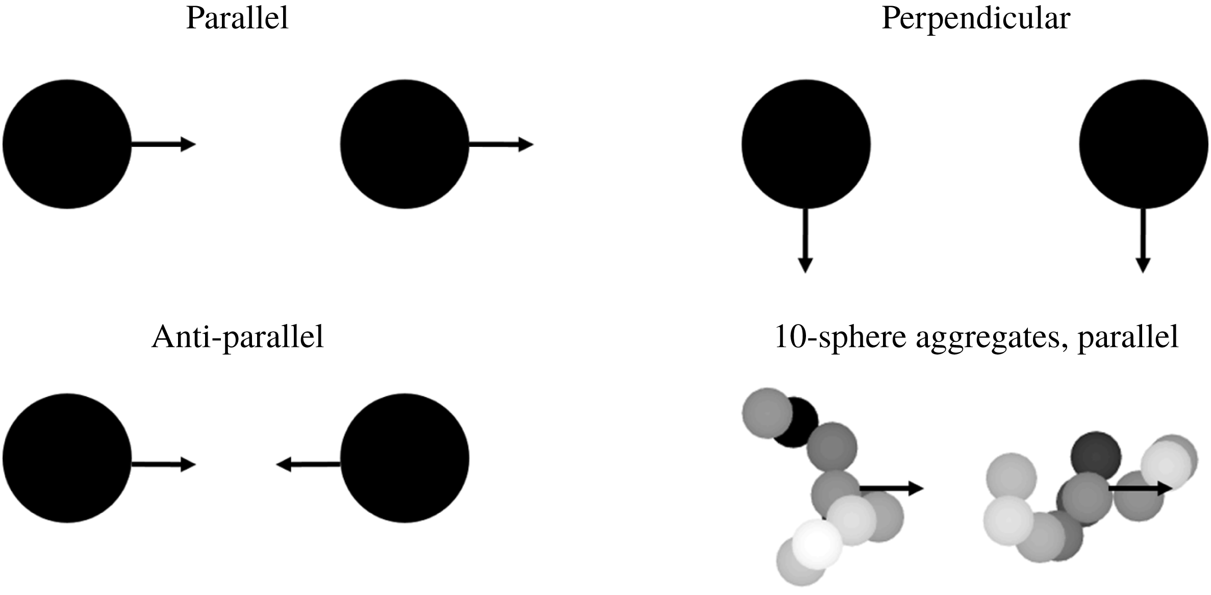
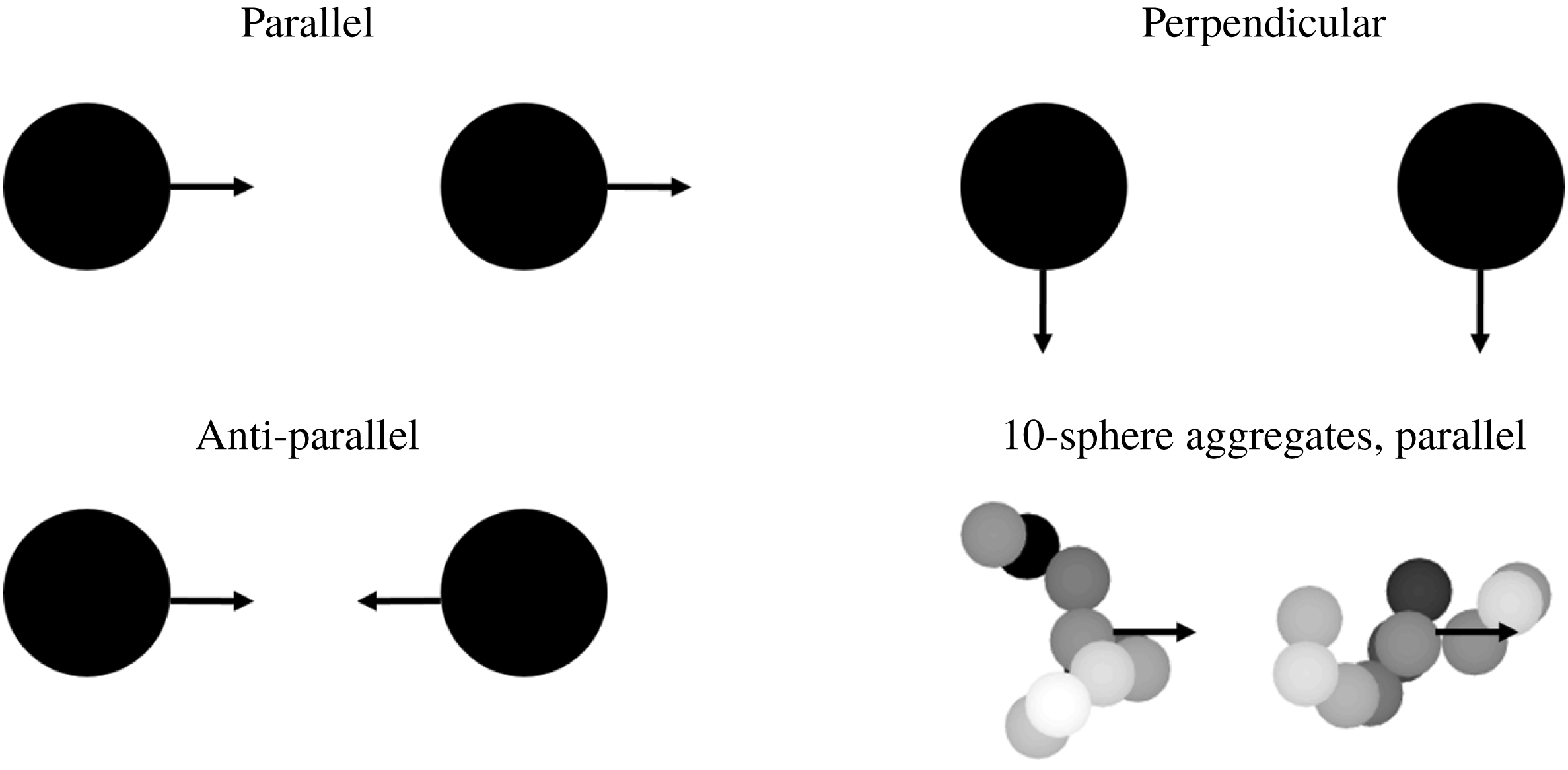
The present study examines the forces exerted by aerosol particles on their neighbours due to hydrodynamic interactions between the particles and the surrounding fluid. We consider both spheres and soot-like fractal aggregates moving parallel, anti-parallel and perpendicular to their line of centres (see figure 1). We employ the extended Kirkwood–Riseman (EKR) method (Corson et al.
Reference Corson, Mulholland and Zachariah2017c
) to solve for the hydrodynamic forces on the particles in the transition flow regime as a function of the separation distance between particles, the Knudsen number (
 $Kn\equiv \unicode[STIX]{x1D706}/a$
, where
 $\unicode[STIX]{x1D706}$
is the gas mean free path and
 $a$
is the sphere radius) of the primary sphere(s) that comprise the particles and the number of primary spheres in the particle. As an example of a situation where hydrodynamic interactions may be significant, we present calculations for the settling velocity of a cloud in an unbounded medium. Throughout this study, we assume the particles are in the creeping flow regime (
 $Re\ll 1$
,
 $Ma\ll 1$
).
Two spheres in the parallel, anti-parallel and perpendicular flow configurations, and two ten-sphere aggregates with random orientations in parallel flow. The descriptor refers to the direction of movement relative to the line connecting the centre of mass of each particle.
2 Theoretical methods
Let us consider two arbitrarily shaped particles immersed in a viscous fluid. Particles 1 and 2 are subjected to external forces
 $\boldsymbol{F}_{1}$
and
 $\boldsymbol{F}_{2}$
, respectively; the centres of mass of the particles are connected by vector
 $\boldsymbol{r}$
. (The forces may result from the presence of the particles in a gravitational or electromagnetic field.) We shall assume that we are in the creeping flow regime, such that inertial forces on both the fluid and the particles are negligible compared to viscous forces. In this regime, there is a linear relationship between the forces on the particles and their velocities,
 $$\begin{eqnarray}\left[\begin{array}{@{}c@{}}\boldsymbol{U}_{1}\\ \boldsymbol{U}_{2}\end{array}\right]=\left[\begin{array}{@{}cc@{}}\unicode[STIX]{x1D648}_{11} & \unicode[STIX]{x1D648}_{12}\\ \unicode[STIX]{x1D648}_{21} & \unicode[STIX]{x1D648}_{22}\end{array}\right]\boldsymbol{\cdot }\left[\begin{array}{@{}c@{}}\boldsymbol{F}_{1}\\ \boldsymbol{F}_{2}\end{array}\right],\end{eqnarray}$$
where
 $\unicode[STIX]{x1D648}_{ij}$
is the mobility tensor that relates the force on particle
 $j$
to the velocity of particle
 $i$
. The mobility tensors are functions of the size and shape of both particles and the distance between them. As
 $r\rightarrow \infty$
, hydrodynamic interactions between particles become negligible. In this case,
 $\unicode[STIX]{x1D648}_{12}=\unicode[STIX]{x1D648}_{21}\approx \unicode[STIX]{x1D7EC}$
, and the mobility tensors
 $\unicode[STIX]{x1D648}_{11}$
and
 $\unicode[STIX]{x1D648}_{22}$
are simply the inverses of the translational friction tensors
 $\unicode[STIX]{x1D729}_{t}$
for particles 1 and 2, defined by the relation
 $$\begin{eqnarray}\boldsymbol{F}=-\unicode[STIX]{x1D729}_{t}\boldsymbol{\cdot }\boldsymbol{U}=-\unicode[STIX]{x1D648}_{ii}^{-1}\boldsymbol{\cdot }\boldsymbol{U}.\end{eqnarray}$$
Our goal is to determine the mobility tensors for particles in the transition flow regime as a function of particle size, shape and separation distance. Before tackling this problem, it is worth considering the simpler case of two spheres in continuum flow. From there, we will describe how one can approach the problem for fractal aggregates in the continuum, before discussing how to apply the extended Kirkwood–Riseman method for particles in the transition regime.
2.1 Two spheres in continuum flow
The instantaneous velocity of two spheres subjected to external forces
 $\boldsymbol{F}_{1}$
and
 $\boldsymbol{F}_{2}$
has been studied by a number of authors (Smoluchowski Reference Smoluchowski1912; Stimson & Jeffery Reference Stimson and Jeffery1926; Burgers Reference Burgers1995; Happel & Brenner Reference Happel and Brenner1965; Batchelor Reference Batchelor1976; Felderhof Reference Felderhof1977). Exact solutions are available for two spheres moving parallel and perpendicular to their line of centres. For arbitrary
 $\boldsymbol{r}$
, the problem can be solved using the method of reflections, whereby the mobility tensors are determined as expansions in powers of the inverse of interparticle separation distance
 $r$
. (See Happel & Brenner (Reference Happel and Brenner1965) for more information about the method of reflections, including its application to the two-sphere problem and to the problem of a particle in a tube.) Since the mobility tensors are symmetric about the line of centres connecting the spheres, we can formally write
 $$\begin{eqnarray}\unicode[STIX]{x1D648}_{ij}=A_{ij}\frac{\boldsymbol{r}\boldsymbol{r}}{r^{2}}+B_{ij}\left(\unicode[STIX]{x1D644}-\frac{\boldsymbol{r}\boldsymbol{r}}{r^{2}}\right),\end{eqnarray}$$
where the non-dimensional coefficients
 $A_{ij}$
and
 $B_{ij}$
can be written as expansions in powers of
 $r^{-n}$
,
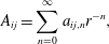 $$\begin{eqnarray}\displaystyle & \displaystyle A_{ij}=\mathop{\sum }_{n=0}^{\infty }a_{ij,n}r^{-n}, & \displaystyle\end{eqnarray}$$
 $$\begin{eqnarray}\displaystyle & \displaystyle B_{ij}=\mathop{\sum }_{n=0}^{\infty }b_{ij,n}r^{-n}. & \displaystyle\end{eqnarray}$$
 $a_{ij,n}$
and
 $b_{ij,n}$
from the method of reflections.
One can include successive terms in the expansions for
 $A_{ij}$
and
 $B_{ij}$
to obtain increasingly accurate results for the mobility tensors. The simplest approach is the point force approximation, where
 $\unicode[STIX]{x1D648}_{ii}=\unicode[STIX]{x1D701}_{i,0}^{-1}\unicode[STIX]{x1D644}$
,
 $\unicode[STIX]{x1D648}_{ij}$
is given by the Oseen tensor (the
 $r^{-1}$
term in (2.5) below),
 $\unicode[STIX]{x1D644}$
is the identity tensor and
 $\unicode[STIX]{x1D701}_{i,0}=6\unicode[STIX]{x03C0}\unicode[STIX]{x1D707}a_{i}$
is the monomer friction coefficient for a sphere with radius
 $a_{i}$
in a fluid with viscosity
 $\unicode[STIX]{x1D707}$
. The next level of approximation yields
 $\unicode[STIX]{x1D648}_{ii}=\unicode[STIX]{x1D701}_{i,0}^{-1}\unicode[STIX]{x1D644}$
and
 $$\begin{eqnarray}\displaystyle \unicode[STIX]{x1D648}_{ij} & = & \displaystyle \frac{1}{8\unicode[STIX]{x03C0}\unicode[STIX]{x1D707}r}\left[\left(\unicode[STIX]{x1D644}+\frac{\boldsymbol{r}\boldsymbol{r}}{r^{2}}\right)+\left(\frac{a_{i}^{2}+a_{j}^{2}}{3r^{2}}\right)\left(\unicode[STIX]{x1D644}-\frac{3\boldsymbol{r}\boldsymbol{r}}{r^{2}}\right)\right]\nonumber\\ \displaystyle & = & \displaystyle \frac{1}{8\unicode[STIX]{x03C0}\unicode[STIX]{x1D707}r}\left[\left(1-\frac{a_{i}^{2}+a_{j}^{2}}{3r^{2}}\right)\frac{2\boldsymbol{r}\boldsymbol{r}}{r^{2}}+\left(1+\frac{a_{i}^{2}+a_{j}^{2}}{3r^{2}}\right)\left(\unicode[STIX]{x1D644}-\frac{\boldsymbol{r}\boldsymbol{r}}{r^{2}}\right)\right]\end{eqnarray}$$
for
 $i\neq j$
. For
 $a_{i}=a_{j}$
, equation (2.5) reduces to the Rotne–Prager–Yamakawa tensor (Rotne & Prager Reference Rotne and Prager1969; Yamakawa Reference Yamakawa1970). Batchelor (Reference Batchelor1976) provides expressions for the mobility tensors accurate to order
 $r^{-5}$
, while Felderhof (Reference Felderhof1977) uses the method of reflections to derive expressions valid to order
 $r^{-7}$
for mixed slip-stick boundary conditions. Results from Felderhof’s interaction tensor are equal to available exact solutions to the two-sphere problem except for very small separation distances (i.e. nearly touching spheres), where higher-order terms become important (Felderhof Reference Felderhof1977).
Note that if sphere 2 is much smaller than sphere 1 (i.e.
 $a_{2}\ll a_{1}$
) and if
 $r$
is large enough that terms higher than order
 $r^{-3}$
are negligible, sphere 2 will simply be advected by the Stokes velocity field generated by sphere 1. This becomes clear solving equation (2.1) for
 $\boldsymbol{U}_{2}$
with
 $\boldsymbol{F}_{2}=\mathbf{0}$
,
 $\boldsymbol{F}_{1}=6\unicode[STIX]{x03C0}\unicode[STIX]{x1D707}a_{1}\boldsymbol{U}_{1}$
and using equation (2.5) for
 $\unicode[STIX]{x1D648}_{21}$
with
 $a_{2}\ll a_{1}$
:
 $$\begin{eqnarray}\boldsymbol{U}_{2}=\left[\frac{3a_{1}}{4r}\left(\unicode[STIX]{x1D644}+\frac{\boldsymbol{r}\boldsymbol{r}}{r^{2}}\right)+\frac{a_{1}^{3}}{4r^{3}}\left(\unicode[STIX]{x1D644}-\frac{3\boldsymbol{r}\boldsymbol{r}}{r^{2}}\right)\right]\boldsymbol{\cdot }\boldsymbol{U}_{1}\equiv \unicode[STIX]{x1D651}(\boldsymbol{r})\boldsymbol{\cdot }\boldsymbol{U}_{1}.\end{eqnarray}$$
Here,
 $\unicode[STIX]{x1D651}(\boldsymbol{r})\boldsymbol{\cdot }\boldsymbol{U}_{1}$
is the Stokes velocity field around a sphere moving with velocity
 $\boldsymbol{U}_{1}$
. We will refer to
 $\unicode[STIX]{x1D651}(\boldsymbol{r})$
as the Stokes tensor.
Any of the above expressions for the mobility tensors can be used to solve the two-sphere problem for arbitrary sphere sizes
 $a_{1}$
and
 $a_{2}$
(provided the continuum approximation is still valid), centre-to-centre distance and orientation
 $\boldsymbol{r}$
and external forces
 $\boldsymbol{F}_{1}$
and
 $\boldsymbol{F}_{2}$
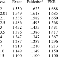
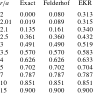
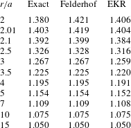
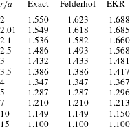
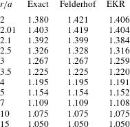
. Table 1–3 show results for the speed of each sphere as a function of separation distance for equal-sized spheres and equal force magnitude. (For
 $a_{1}=a_{2}$
, the speeds of the spheres are equal.) The tables include results for the exact solutions to the two-sphere problem (Stimson & Jeffery Reference Stimson and Jeffery1926; Brenner Reference Brenner1961; Goldman et al.
Reference Goldman, Cox and Brenner1966), the mobility expression of Felderhof for stick boundary conditions (Felderhof Reference Felderhof1977), and our EKR method (i.e. using the Stokes tensor) for the three cases shown in figure 1. In all cases, the Stokes tensor results are in very good agreement (less than 1 % difference) with the exact results for
 $r/a>5$
. As expected, the error is more significant for smaller separation distances because the Stokes tensor does not include terms of order
 $r^{-4}$
and higher and because there is a missing factor of 2 in the
 $r^{-3}$
term.
Speed of two spheres moving parallel to their line of centres, relative to the speed of isolated spheres subjected to the same external force. The EKR or Stokes tensor solution refers to
 $\unicode[STIX]{x1D648}_{ii}=\unicode[STIX]{x1D701}_{i,0}^{-1}$
and
 $\unicode[STIX]{x1D648}_{ij}=\unicode[STIX]{x1D701}_{i,0}^{-1}\unicode[STIX]{x1D651}(\boldsymbol{r})$
, where
 $\unicode[STIX]{x1D651}(\boldsymbol{r})$
is defined in (2.6). The Felderhof tensors (Felderhof Reference Felderhof1977) are accurate to order
 $r^{-7}$
. The exact solution is given by Stimson & Jeffery (Reference Stimson and Jeffery1926).
Speed of two spheres moving anti-parallel to their line of centres, relative to the speed of isolated spheres subjected to the same external force. The exact solution is given by Brenner (Reference Brenner1961).
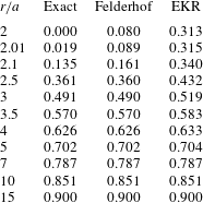
Speed of two spheres moving perpendicular to their line of centres, relative to the speed of isolated spheres subjected to the same external force. The exact solution is given by Goldman et al. (Reference Goldman, Cox and Brenner1966).
2.2 Aggregates in continuum flow
Experiments and simulations have shown that particles formed by diffusion-limited cluster aggregation have a fractal morphology with fractal dimension
 $d_{f}\approx 1.78$
and prefactor
 $k_{0}\approx 1.3$
(Sorensen Reference Sorensen2011). These parameters relate the radius of gyration to the number of spheres in the aggregate,
 $$\begin{eqnarray}N=k_{0}\left(\frac{R_{g}}{a}\right)^{d_{f}}.\end{eqnarray}$$
Notable examples of DLCA aggregates include soot, as well as titania and other ceramic powders synthesized in aerosol flame reactors (Pratsinis Reference Pratsinis1998).
In the previous section, we reviewed how one can solve the two-sphere problem to various levels of approximation. We now describe how to use a similar approach for aggregates.
In approaches based on Kirkwood–Riseman theory (Kirkwood & Riseman Reference Kirkwood and Riseman1948), one uses any of the above expressions for the interactions between pairs of spheres to determine the force on a macromolecule or particle consisting of
 $N$
spherical subunits. The resulting system of equations is analogous to (2.1):
 $$\begin{eqnarray}-\boldsymbol{U}_{i}=\mathop{\sum }_{j=1}\unicode[STIX]{x1D648}_{ij}\boldsymbol{\cdot }\boldsymbol{F}_{j}.\end{eqnarray}$$
Here,
 $\boldsymbol{F}_{j}$
is the force exerted by the fluid on the
 $j$
th primary sphere in an aggregate, which is unknown, whereas in (2.1)
 $\boldsymbol{F}_{j}$
represents the known external force on the
 $j$
th particle in a two-particle system. (The negative sign appearing in (2.8) is a consequence of the shift from the force exerted by the particle – as in (2.1) – to the force exerted on the
 $i$
th primary sphere by the fluid.) To determine the force on a macromolecule or particle whose subunits have velocities
 $\boldsymbol{U}_{i}$
, one solves the above linear system for the force on each sphere, then sums over all spheres to get the total force. Alternatively, if the total external force on the particle is given (e.g. gravity or the force on charged particle in an electric field), one can solve (2.8) iteratively to get the particle velocity such that the calculated force distribution is consistent with the total force.
KR-based treatments rely on the underlying linearity of the Stokes flow equations. In their original formulation, Kirkwood & Riseman (Reference Kirkwood and Riseman1948) set
 $\unicode[STIX]{x1D648}_{ij}=\unicode[STIX]{x1D6FF}_{ij}\unicode[STIX]{x1D701}_{i,0}^{-1}+(1-\unicode[STIX]{x1D6FF}_{ij})\unicode[STIX]{x1D64F}_{ij}$
, where
 $\unicode[STIX]{x1D6FF}_{ij}$
is the Kronecker delta and
 $\unicode[STIX]{x1D64F}_{ij}$
is the Oseen tensor. Later applications of KR theory (García de la Torre & Rodes Reference García de la Torre and Rodes1983; Chen, Deutch & Meakin Reference Chen, Deutch and Meakin1984; Lattuada, Wu & Morbidelli Reference Lattuada, Wu and Morbidelli2003) replace the Oseen tensor with the Rotne–Prager–Yamakawa tensor. One can use higher-order approximations for the mobility tensors (e.g. the Felderhof expressions); one can also account for multi-body effects using mobility tensors derived by Mazur & Van Saarloos (Reference Mazur and Van Saarloos1982). However, Carrasco & García de la Torre (Reference Carrasco and García de la Torre1999) have shown that using these more rigorous methods to calculate particle friction and diffusion tensors offers little improvement over using KR-theory with the Rotne–Prager–Yamakawa tensor.
One can use the same KR-based methods to determine the forces between two aggregates: one again solves the system of equations given by (2.8), but now one sums over the spheres in each aggregate to determine the total hydrodynamic force. Again, one can perform this calculation for aggregates with specified velocities or specified external forces. By comparing this result to the force on an isolated aggregate, one can determine the effect of the second aggregate on the mobility of the first.
2.3 Extended Kirkwood–Riseman theory
The previous subsections have focused on situations where the continuum approach is valid. For particles consisting of spheres with diameters of the order of tens of nanometres moving through air at standard temperature and pressure (
 $\unicode[STIX]{x1D706}\approx 67$
nm), one cannot use the expressions for interactions between particles in the continuum, but one can use the same general (2.8) relating the velocity of particles in the transition regime to the drag forces exerted on the particles by the fluid. One only needs to determine the mobility tensors as a function of the primary sphere Knudsen numbers.
Noting that the Stokes velocity tensor provides a reasonable approximation for the mobility tensor between two spheres in the continuum (see tables 1–3), we (Corson et al. Reference Corson, Mulholland and Zachariah2017c ) proposed replacing the Stokes velocity tensor with a Knudsen-number-dependent velocity tensor obtained by solving the Bhatnagar–Gross–Krook (BGK) equation (Bhatnagar, Gross & Krook Reference Bhatnagar, Gross and Krook1954) for flow around a sphere. (The BGK equation is a simplified, linearized version of the Boltzmann transport equation that is valid for near-equilibrium situations (Kogan Reference Kogan1958). Velocities calculated using the BGK equation compare well to solutions of the linearized Boltzmann equation (Loyalka Reference Loyalka1992; Takata, Sone & Aoki Reference Takata, Sone and Aoki1993).) The resulting set of equations relating the sphere velocities to the drag is
 $$\begin{eqnarray}\boldsymbol{F}_{i}=-\unicode[STIX]{x1D701}_{i,0}(Kn_{i})\boldsymbol{U}_{i}-\unicode[STIX]{x1D701}_{i,0}(Kn_{i})\mathop{\sum }_{i\neq j}^{N}\unicode[STIX]{x1D701}_{j,0}^{-1}(Kn_{j})\unicode[STIX]{x1D651}_{ij}(Kn_{j})\boldsymbol{\cdot }\boldsymbol{F}_{j}.\end{eqnarray}$$
Here,
 $N$
is the number of spheres in the system and
 $\unicode[STIX]{x1D651}_{ij}$
is the velocity tensor around a sphere with Knudsen number
 $Kn_{j}$
(i.e. the transition regime analogue of the Stokes tensor defined in (2.6)). The velocity tensor is a function of the vector connecting the centres of spheres
 $i$
and
 $j$
(see Corson et al.
Reference Corson, Mulholland and Zachariah2017c
for futher details). Note that the force on sphere
 $i$
depends on the friction coefficient for sphere
 $i$
and the velocities around the other
 $j$
spheres.
Our previous work (Corson, Mulholland & Zachariah Reference Corson, Mulholland and Zachariah2017a ; Corson et al. Reference Corson, Mulholland and Zachariah2017c ) has demonstrated that using the velocity and drag results from the BGK equation and solving equation (2.9) yields accurate results for the translational friction coefficient of fractal aggregates across the entire Knudsen regime. This suggests that the EKR method can be used to determine the hydrodynamic forces between particles in the kinetic regime.
2.4 Point force approach
If one is only concerned about interactions between widely separated particles, the analysis can be greatly simplified by treating the particles as point forces. In the continuum, the flow field generated by the point force is often called the Stokeslet and can be written as
 $$\begin{eqnarray}\boldsymbol{u}(\boldsymbol{r})=\frac{1}{8\unicode[STIX]{x03C0}\unicode[STIX]{x1D707}r}\left(\unicode[STIX]{x1D644}+\frac{\boldsymbol{r}\boldsymbol{r}}{r^{2}}\right)\boldsymbol{\cdot }\boldsymbol{F},\end{eqnarray}$$
where the term multiplying the point force is the Oseen tensor. If the object is a sphere,
 $\boldsymbol{F}$
is given by Stokes’ law, and (2.10) gives the flow field for large
 $r$
. Interestingly, this flow field is valid regardless of the shape of the object exerting the force on the fluid. This means that the flow field far from an object looks like the flow around a sphere exerting the same force on the fluid as the object, even when the object is highly non-spherical. This behaviour is due to viscous effects in the fluid.
Based on the preceding discussion, we can determine the interactions between the aggregates using a point force approach, such that the total hydrodynamic force on each aggregate can be obtained by simultaneously solving the following equations:
 $$\begin{eqnarray}\boldsymbol{F}_{i}=-\unicode[STIX]{x1D729}_{i,0}\boldsymbol{\cdot }\boldsymbol{U}_{i}-\unicode[STIX]{x1D729}_{i,0}\boldsymbol{\cdot }\mathop{\sum }_{i\neq j}^{N}\left[\frac{1}{8\unicode[STIX]{x03C0}\unicode[STIX]{x1D707}r_{ij}}\left(\unicode[STIX]{x1D644}+\frac{\boldsymbol{r}\boldsymbol{r}}{r^{2}}\right)\right]\boldsymbol{\cdot }\boldsymbol{F}_{j}.\end{eqnarray}$$
Here,
 $N$
is the number of aggregates in the system,
 $\boldsymbol{r}_{ij}$
is the vector between the centre of mass of
 $i$
th and
 $j$
th aggregates and
 $\unicode[STIX]{x1D729}_{i,0}$
is the translational friction tensor for aggregate
 $i$
when it is alone in an infinite fluid. Mackaplow & Shaqfeh (Reference Mackaplow and Shaqfeh1998) demonstrated that the point force approach applied to the problem of sedimentation of fibres in a semi-dilute homogeneous suspension yields results similar to those of a more sophisticated Monte Carlo simulation of the problem.
The point force approach should also be valid in the transition regime, albeit with a Knudsen-number-dependent hydrodynamic interaction tensor in place of the Oseen tensor. In fact, the transition regime interaction tensor should have the same form as the Oseen tensor but with a different coefficient in place of
 $1/8$
. This is because the fluid velocity far from a sphere has the general form
 $$\begin{eqnarray}\boldsymbol{u}(\boldsymbol{r})=-\frac{c_{1}(Kn)}{2}\frac{a}{r}\left(\unicode[STIX]{x1D644}+\frac{\boldsymbol{r}\boldsymbol{r}}{r^{2}}\right)\boldsymbol{\cdot }\boldsymbol{U}=-\frac{c_{1}(Kn)}{2\unicode[STIX]{x1D701}_{i,0}(Kn)}\frac{a}{r}\left(\unicode[STIX]{x1D644}+\frac{\boldsymbol{r}\boldsymbol{r}}{r^{2}}\right)\boldsymbol{\cdot }\boldsymbol{F},\end{eqnarray}$$
where
 $\boldsymbol{U}$
is the sphere velocity,
 $\boldsymbol{F}$
is the force exerted by the sphere on the fluid and
 $c_{1}(Kn)$
is a coefficient that can be obtained by solving the BGK or linearized Boltzmann equation for flow around a sphere (Takata et al.
Reference Takata, Sone and Aoki1993; Corson et al.
Reference Corson, Mulholland and Zachariah2017c
). In the continuum,
 $c_{1}=-3/2$
, and (2.12) reduces to (2.10).
Substituting (2.12) for the Oseen tensor in (2.11), we get the following result for a system of
 $N$
aerosol aggregates:
 $$\begin{eqnarray}\boldsymbol{F}_{i}=-\unicode[STIX]{x1D729}_{i,0}(Kn_{i})\boldsymbol{\cdot }\boldsymbol{U}_{i}-\unicode[STIX]{x1D729}_{i,0}(Kn_{i})\boldsymbol{\cdot }\mathop{\sum }_{i\neq j}^{N}\left[-\frac{c_{1}(Kn_{j,eff})}{2\unicode[STIX]{x1D701}_{j,0}}\left(\unicode[STIX]{x1D644}+\frac{\boldsymbol{r}\boldsymbol{r}}{r^{2}}\right)\right]\boldsymbol{\cdot }\boldsymbol{F}_{j}.\end{eqnarray}$$
Here,
 $a_{j,eff}$
is the radius and
 $Kn_{j,eff}=\unicode[STIX]{x1D706}/a_{j,eff}$
the Knudsen number of a sphere with friction coefficient
 $\unicode[STIX]{x1D701}_{j,0}=|\unicode[STIX]{x1D729}_{j,0}(Kn_{j})\boldsymbol{\cdot }\boldsymbol{U}_{j}/\boldsymbol{U}_{j}|$
, where
 $\unicode[STIX]{x1D729}_{j,0}(Kn_{j})$
is the friction tensor for aggregate
 $j$
alone in an infinite fluid and
 $\boldsymbol{U}_{j}$
is the velocity of aggregate
 $j$
. One solves implicitly for the effective radius of the cluster,
 $$\begin{eqnarray}\unicode[STIX]{x1D701}_{j,0}(Kn_{j,eff})=\frac{6\unicode[STIX]{x03C0}\unicode[STIX]{x1D707}a_{j,eff}}{C_{c}(\unicode[STIX]{x1D706}/a_{j,eff})},\end{eqnarray}$$
where
 $C_{c}$
is the Cunningham slip correction factor. We have explicitly stated the dependence of the aggregate friction tensors on the Knudsen number of the primary spheres in the aggregate; of course, the friction tensor also depends on the number of spheres in the aggregate and the configuration of those spheres. Note that (2.14) accounts for the orientation of each cluster through the use of the friction tensors, and by determining the effective radius based on the drag force for a particular aggregate orientation relative to the flow. However, one can further simplify (2.13) by replacing the friction tensors with the scalar friction coefficients based on orientation averages for the particles. This simplification is justified for aerosol particles due to the randomizing effects of Brownian forces.
To apply the point force approximation for a system of aggregates in the transition regime, one must first determine the friction tensor for each aggregate (e.g. by solving (2.9)). Next, one must determine the effective sphere radius for each aggregate. One obtains the coefficient
 $c_{1}(Kn_{j,eff})$
for each aggregate from a table of BGK or linearized Boltzmann results. With this information, one can solve (2.13) for the hydrodynamic forces on the system of aggregates. Again, one can replace the friction tensors with the scalar friction coefficient for each aggregate. One can use the adjusted sphere method (Dahneke Reference Dahneke1973; Zhang et al.
Reference Zhang, Thajudeen, Larriba, Schwartzentruber and Hogan2012) or our EKR method (Corson et al.
Reference Corson, Mulholland and Zachariah2017c
) to quickly determine the friction coefficient for each aggregate, which significantly reduces the complexity of the problem.
Using the point force approach is beneficial because one can significantly reduce the number of simultaneous equations that one must solve compared to considering the pairwise interactions among all of the spheres in all of the aggregates. This is especially useful if one is considering a system consisting of identical aggregates (such that one need only determine the friction tensor once) or if one is considering interactions between coagulating aerosols (such that the friction tensors for the aggregates remain constant until two particles coagulate, at which point one need only calculate the friction tensor for the new particle). While the point force approach is strictly valid only for widely separated particles, we will show in the following section that this approach provides reasonable results even when the aggregates are fairly close together.
3 Two-particle results
We have used our extended Kirkwood–Riseman method (2.9) to determine the hydrodynamic forces between two aggregates moving parallel, anti-parallel and perpendicular to their line of centres in the transition flow regime. We start by considering two spheres, then move to the case of two fractal aggregates. For simplicity, we will focus on cases where the two particles are identical, though we do consider the effects of orientation for the aggregate calculations.
3.1 Sphere results
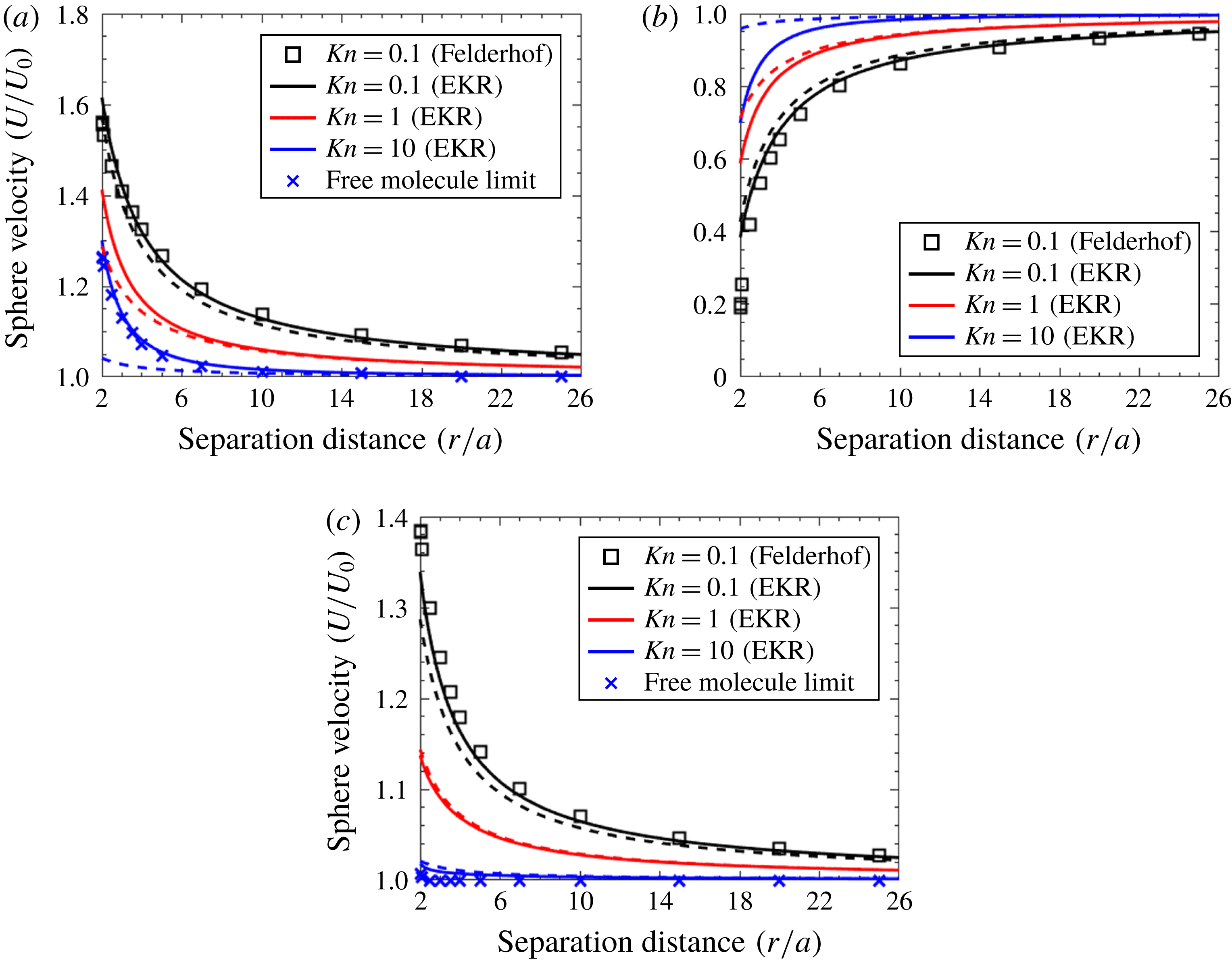
Figure 2 shows the results for two spheres moving parallel, anti-parallel and perpendicular to their line of centres. Results are plotted as a function of separation distance for three different Knudsen numbers. Here, we show the ratio of the velocity of each sphere subjected to the same external force (albeit in opposite directions for the anti-parallel case) to the velocity it would have if was alone in an infinite medium subjected to the same force. Note that one can obtain the effect on the hydrodynamic force for specified velocity by taking the inverse of the results in figure 2. The figure includes results for both the EKR method (§ 2.3, solid lines) and the point force method (§ 2.4, dashed lines). We also present the velocities calculated using Felderhof’s mobility tensors (Felderhof Reference Felderhof1977) for mixed slip-stick boundary conditions for
 $Kn=0.1$
and the velocities in the free molecular limit. The Felderhof tensors are accurate to order
 $r^{-7}$
and are expected to yield nearly exact results except for very small separation distances for this near-continuum situation. We have obtained the free molecule results using an algorithm similar to the one described by Mackowski (Reference Mackowski2006).
Speed of two spheres moving (a) parallel, (b) anti-parallel and (c) perpendicular to their line of centres, relative to the speed of isolated spheres subjected to the same external force. Results using the mobility tensors of Felderhof (Reference Felderhof1977) for mixed slip-stick boundary conditions are shown for comparison to the
 $Kn=0.1$
results. Note that for the Felderhof calculations we use a slip length of 0.9875 times the gas mean free path based on the best-estimate results of Loyalka (Reference Loyalka1990). Results in the free molecular limit are shown for comparison to the
 $Kn=10$
results for the parallel and perpendicular configurations. Solid lines represent our EKR results (2.9), while dashed lines represent point force results (2.13) for each Knudsen number.
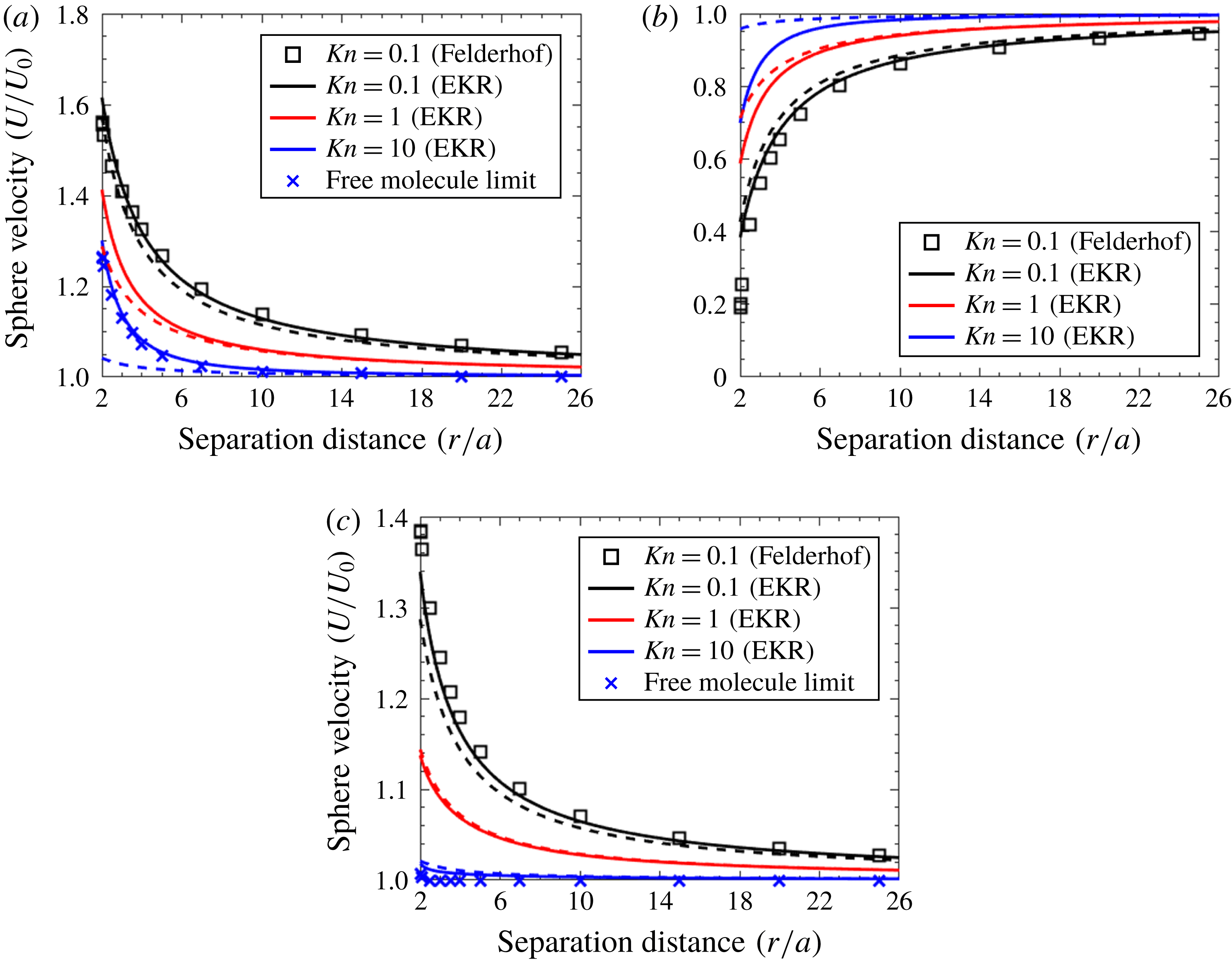
The figure shows that our EKR results are in good agreement with the Felderhof mobility tensor results for near-continuum conditions (or near-stick boundary conditions, in the case of the Felderhof results). For
 $r/a>3$
, the two methods yield results within about 2 % of each other; this is not surprising, since the higher-order terms in the expansions representing the mobility tensors decay quickly with increasing separation. The error is still fairly low (
 ${<}8\,\%$
) for touching spheres moving parallel and perpendicular to their line of centres but is much more significant for the anti-parallel configuration. This is because our EKR method ignores lubrication forces between the particles, whereas Felderhof’s mobility tensors partially account for these forces through the higher-order terms in the expansion.
As expected, the strength of the hydrodynamic interactions between spheres decreases with increasing Knudsen number. For the perpendicular configuration, the two spheres behave almost as if they are isolated even when they are in contact at high Knudsen number; the effect is more important in the parallel and anti-parallel configurations, likely due to direct shielding of incoming gas molecules by the other sphere and molecules that collide with both spheres before colliding with other gas molecules. Our results at large Knudsen number are in good agreement with the free molecule results for the parallel configuration. The agreement is not as good for spheres with
 $Kn=10$
in perpendicular flow for small separation distances, though the interaction strength quickly becomes negligible as the separation distance increases.
As we saw in the previous section, the long-range hydrodynamic interactions have a
 $r^{-1}$
dependence in the continuum, as given by the Oseen tensor. The
 $r^{-1}$
dependence is also evident in our transition regime results in figure 2. At large separation distances, the point force results are nearly identical to the EKR results, as expected.
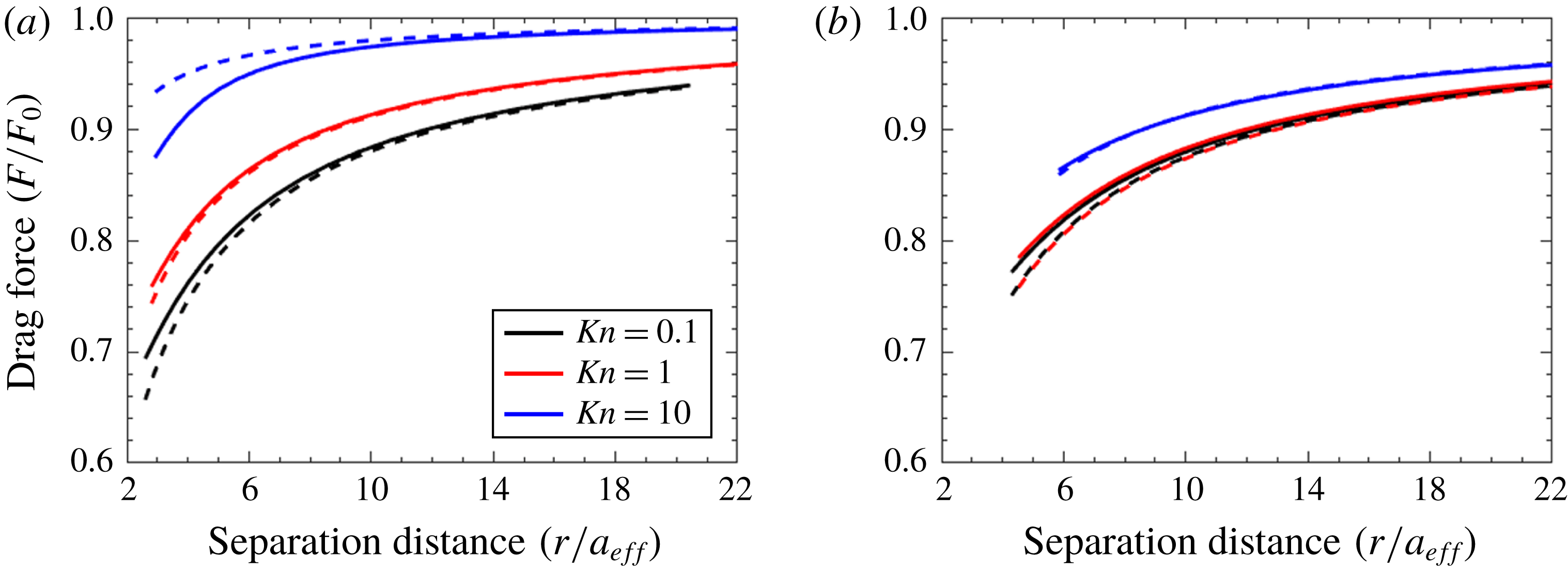
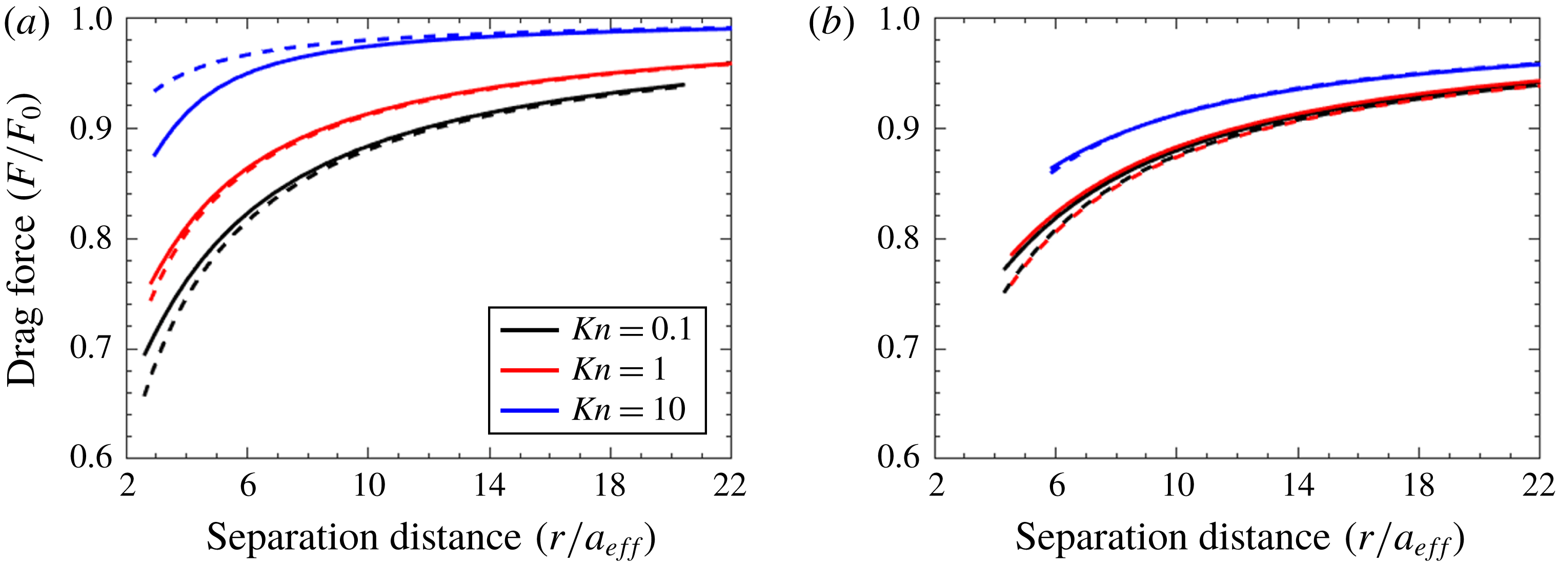
Hydrodynamic force on an aggregate as a function of the distance between its centre of mass and the centre of mass of an identical aggregate. (a) Shows results for
 $N=10$
, while (b) shows results for
 $N=1000$
. The solid lines represent the full EKR results (2.9), while the dotted lines represent the point force results (2.13). The drag force is normalized by the drag on one of the aggregates in an infinite fluid, while the separation distance is presented as the number of effective sphere radii (i.e. the radius of a sphere experiencing drag force
 $F_{0}$
) between the centres of mass of the particles.
3.2 Aggregate results
Figure 3 shows the results for two aggregates moving parallel to their line of centres. Results are shown for two aggregates with 10 spheres each and for two aggregates with 1000 spheres. The results are presented as the ratio of the drag on one of the aggregates to the drag on that aggregate when it is alone in an infinite fluid. Solid lines represent the full EKR solution (2.9), while the dotted lines represent the point force results (2.13). From the figures, the point force solution is sufficiently accurate for all but the closest separations, which greatly simplifies any analysis of the effects of hydrodynamic interactions between aggregates. Also, the aggregates exhibit more continuum-like behaviour as the number of spheres in the aggregate increases, which is analogous to the behaviour we have observed for the translational and rotational friction coefficients of DLCA aggregates (Corson et al. Reference Corson, Mulholland and Zachariah2017a ; Corson, Mulholland & Zachariah Reference Corson, Mulholland and Zachariah2018a ).
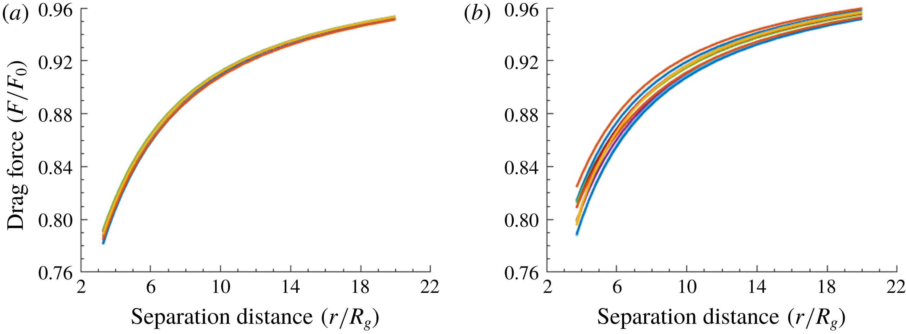
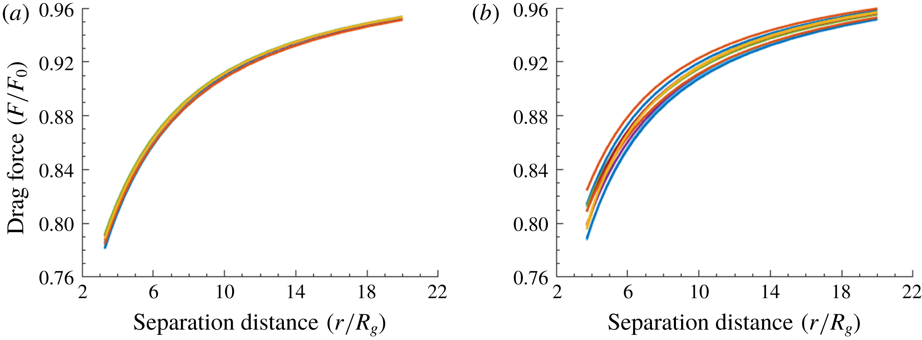
Figure 3 presents the results for aggregates with a fixed orientation. Figure 4 explores the effect of orientation on the reduction in the drag force for
 $N=500$
and a primary sphere Knudsen number of 2.7. Results are shown for two aggregates with a shape anisotropy
 $A_{31}=2.0$
and for two aggregates with
 $A_{31}=6.5$
, where
 $A_{31}$
is the ratio of the largest to smallest eigenvalues of the inertia tensor of the particle. Since each cluster in the first pair is fairly isotropic (
 $A_{31}$
near unity), there is little change in the hydrodynamic force on each cluster as the particles rotate. In contrast, there is a noticeable difference in hydrodynamic force as the more anisotropic particles rotate. This is especially true for small separation distances. Note that in each case we normalize by the force on the particle for that particular orientation.
Effects of orientation on the hydrodynamic force on one of two 500-sphere aggregates with primary sphere
 $Kn=2.7$
(sphere radius of 25 nm at room temperature), calculated using the EKR method. Results are presented as the ratio of the force on an aggregate for the specified separation distance to the force on the aggregate alone in an infinite fluid at a particular orientation. Each line represents a randomly chosen orientation for each aggregate in the two-aggregate system. (a) An aggregate with anisotropy
 $A_{31}=2.0$
, and (b) an aggregate with
 $A_{31}=6.5$
.
4 Discussion
Our results show that hydrodynamic interactions between particles in the transition flow regime are significant for small separation distances and still noticeable at separations of more than 10 sphere diameters or 20 times the radius of gyration of an aggregate. The effect is stronger near the continuum than near the free molecule regime and stronger for parallel and anti-parallel configurations than for perpendicular configurations for all particle sizes.
With that said, hydrodynamic interactions may have little effect on measurable quantities of interest (e.g. viscosity and deposition rates) except in very dense aerosol systems, due to the large average particle separations in most practical systems. (The situation is less clear for coagulation, as we discuss below.) As an example, consider an aerosol consisting of spherical particles with volume fraction
 $\unicode[STIX]{x1D719}$
. The average spacing between the particles is
 $\bar{L}/a=(4\unicode[STIX]{x03C0}/3\unicode[STIX]{x1D719})^{1/3}$
, so at a relatively high volume fraction of
 $10^{-4}$
, the average spacing approximately 35 sphere radii. Near the continuum, the hydrodynamic force between spheres is less than 5 % of the external force generating the sphere motion; this ratio decreases with increasing Knudsen number.
Of course, aerosol particles are not arranged in a grid, with equal spacing between particles. Still, the expressions for the settling velocity and suspension viscosity in the introduction account for the probability distribution of sphere locations in a suspension. Thus, interparticle hydrodynamic interactions have very little impact on these parameters for an aerosol consisting of spherical particles at typical volume fractions.
The situation is more complicated for fractal aggregates due to the difference between the fractal dimension and the spatial dimension. To understand why, let us consider an aerosol consisting of a large number of identical
 $N$
-sphere aggregates. The average distance between the centres of mass of the aggregates is simply
 $\bar{L}/a=(4\unicode[STIX]{x03C0}N/3\unicode[STIX]{x03C0})^{1/3}$
, regardless of the fractal dimension of the aggregates. Now let us rewrite the average spacing in terms of the radius of gyration:
 $$\begin{eqnarray}\frac{\bar{L}}{R_{g}}=\frac{(4\unicode[STIX]{x03C0}N/3\unicode[STIX]{x1D719})^{1/3}}{(N/k_{0})^{1/d_{f}}}=\left(\frac{4\unicode[STIX]{x03C0}k_{0}^{3/d_{f}}}{3\unicode[STIX]{x1D719}}\right)^{1/3}N^{(d_{f}-3)/3d_{f}}.\end{eqnarray}$$
Here,
 $k_{0}$
and
 $d_{f}$
are the prefactor and fractal dimension of the aggregates. For DLCA aggregates (
 $k_{0}\approx 1.3$
,
 $d_{f}\approx 1.78$
), and for a volume fraction of
 $10^{-4}$
, the average spacing between aggregates is 24 radii of gyration for
 $N=10$
and 8.3 radii of gyration for
 $N=1000$
. Since the radius of gyration is approximately equal to the effective hydrodynamic radius of a particle in continuum flow, we can consult the near-continuum results in figure 3 to estimate the hydrodynamic force between the aggregates in the parallel flow configuration at these average separation distances. For
 $N=1000$
, the drag force for the parallel configuration is approximately 85 % of the drag at infinite separation distance for
 $Kn=0.1$
. Compare this to the result for a system of spheres in continuum flow, where the average separation is 34 radii, and the force at this separation is 96 % of the force at infinite separation for
 $Kn=0.1$
.
On the other hand, hydrodynamic interactions between particles may have a noticeable effect on coagulation rates. This is certainly true for dense aerosol systems (Sorensen et al. Reference Sorensen, Hageman, Rush, Huang and Oh1998; Sorensen & Chakrabarti Reference Sorensen and Chakrabarti2011), but some studies of particles in the continuum suggest that hydrodynamic interactions may have a noticeable effect on the coagulation rate predicted by the Smoluchowski equation even for dilute systems (see Matsuoka et al. Reference Matsuoka, Fukasawa, Higashitani and Yamamoto2012). Since particles must approach each other in order to coagulate, one might expect that hydrodynamic interactions have some effects on either the coagulation rate or the structure of the particles formed. However, hydrodynamic interactions are typically ignored when determining particle coagulation rates (Mountain, Mulholland & Baum Reference Mountain, Mulholland and Baum1986; Heine & Pratsinis Reference Heine and Pratsinis2007; Lattuada Reference Lattuada2011; Heinson et al. Reference Heinson, Pierce, Sorensen and Chakrabarti2014); this is especially for aerosol systems. Furthermore, previous studies on coagulation have been largely confined to the free molecule or continuum regimes; our EKR approach allows one to determine the translational and rotational friction tensors for aggregates in the transition regime (Corson, Mulholland & Zachariah Reference Corson, Mulholland and Zachariah2017b ; Corson et al. Reference Corson, Mulholland and Zachariah2017c ), including the effects of an external force field on particle mobility (Corson, Mulholland & Zachariah Reference Corson, Mulholland and Zachariah2018b ). Thus, one could use either our EKR method or the point force method needed to determine the hydrodynamic and Brownian forces on each particle, which are affected by hydrodynamic interactions.
4.1 Aerosol clouds
One interesting problem involving hydrodynamic interactions among particles is the settling of an unbounded aerosol cloud in a gravitational field. This problem has been studied extensively for spherical particles in the continuum (for a small sample, refer to the works of Burgers (Reference Burgers1995) or to Fuchs (Reference Fuchs1964)). The behaviour of the particle cloud depends on the volume fraction of particles in the cloud. For sufficiently low volume fractions, the particles behave as if they are isolated, as one would expect. In this case, the velocity of each particle is obtained by balancing the gravitational force
 $F_{g}$
with the drag force,
 $$\begin{eqnarray}v_{s1}=\frac{F_{g}}{\unicode[STIX]{x1D701}_{0}}.\end{eqnarray}$$
For high volume fractions, the particles entrain the surrounding fluid, and the cloud behaves as a gas bubble with the same viscosity as the fluid surrounding the cloud (Fuchs Reference Fuchs1964; Burgers Reference Burgers1995). In this case, the velocity of the cloud is given by
 $$\begin{eqnarray}v_{s2}=\frac{\frac{4}{3}\unicode[STIX]{x03C0}R^{3}nF_{g}}{5\unicode[STIX]{x03C0}\unicode[STIX]{x1D707}R}=\frac{4R^{2}nF_{g}}{15\unicode[STIX]{x1D707}},\end{eqnarray}$$
where
 $R$
is the radius of the cloud and
 $n$
is the number concentration of particles. In the first equality, we explicitly write the velocity as the ratio between the total gravitational force on the cloud and the drag on a spherical bubble with equal viscosity in the inner and outer fluids. The particles behave as if they are isolated when
 $v_{s2}/v_{s1}\ll 1$
and as a cloud with velocity given by (4.3) when
 $v_{s2}/v_{s1}\gg 1$
(Fuchs Reference Fuchs1964).
The above analysis is applicable for aggregates in continuum flow, with a few important caveats. First, one must use appropriate values for the gravitational and drag forces on the aggregate. Second, the effects of the aggregates on the effective viscosity of the cloud must be negligible; of course, this restriction also applies to the aforementioned case of spherical particles. Additionally, we will ignore the effects of hydrodynamic interactions on the orientation of the aggregates. We will address this restriction in more detail in the following section. With the above caveats, we can write the ratio
 $v_{s2}/v_{s1}$
for a cloud consisting of identical
 $N$
-sphere aggregates as
 $$\begin{eqnarray}\frac{v_{s2}}{v_{s1}}=\frac{6\unicode[STIX]{x1D719}\unicode[STIX]{x1D701}_{0}^{\star }R^{2}}{5Na^{2}},\end{eqnarray}$$
where
 $\unicode[STIX]{x1D701}_{0}^{\star }\equiv 6\unicode[STIX]{x03C0}\unicode[STIX]{x1D707}a\unicode[STIX]{x1D701}_{0}$
is the non-dimensional friction coefficient for the aggregate when it is alone in an infinite fluid. Note that the volume fraction is simply the number density times the volume of one aggregate, i.e.
 $\unicode[STIX]{x1D719}=(4/3)\unicode[STIX]{x03C0}a^{3}Nn$
.
Now, we will consider whether or not the above analysis applies to particles – whether spheres or aggregates – in the transition regime. (Again, if we wish to consider aggregates, our analysis is subject to the caveats mentioned above for particles in continuum flow.) To do so, we will consider an idealized situation: a cloud of radius
 $R$
that consists of identical particles in a cubic lattice. For this problem, each particle experiences the same external force, so we can directly solve (2.13) for the velocity of each particle in the cloud,
 $\boldsymbol{U}_{i}$
. If Fuchs analysis is applicable for particles in the transition regime, then our calculated velocity should approach that given by (4.3) when the ratio
 $v_{s2}/v_{s1}$
(4.4) is much greater than unity and should approach
 $F_{g}/\unicode[STIX]{x1D701}_{0}$
when the result of (4.4) is much less than unity.
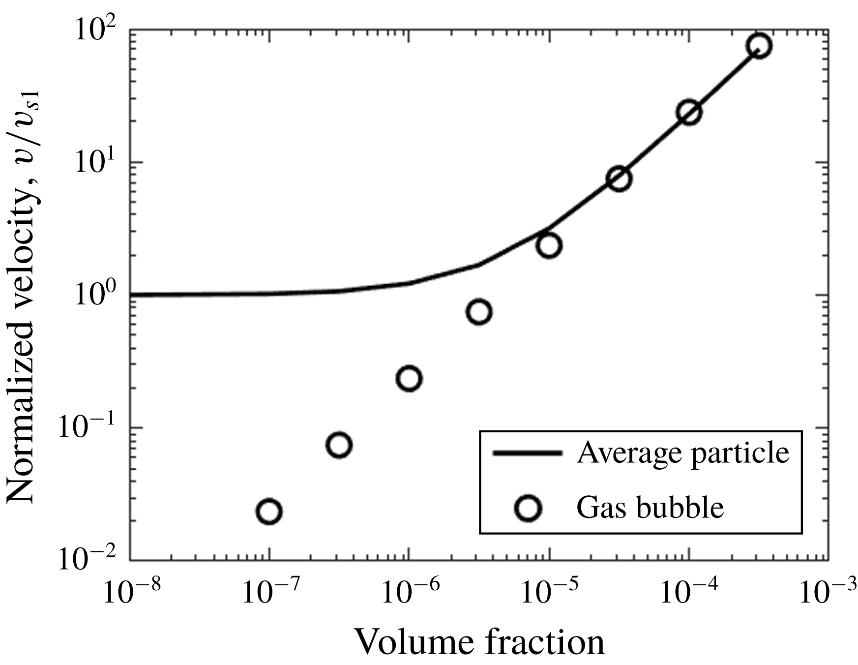
Figure 5 shows the average particle velocity in the aerosol cloud as a function of the aerosol volume fraction. The calculations are performed for 25 nm radius spheres (
 $Kn=2.7$
) and a 25 m radius cloud. Average velocities are normalized by the settling velocity of an isolated sphere (i.e. by
 $v_{s1}$
). The figure shows that for
 $v_{s2}/v_{s1}\gg 1$
, the average velocity of spheres in the cloud approaches
 $v_{s2}$
, and for
 $v_{s2}/v_{s1}\ll 1$
, the spheres behave as if they are isolated.
Average velocity for a cloud of spheres, normalized by the settling velocity of a single particle,
 $v_{s1}$
. The velocity of a gas bubble having the same volume fraction and cloud radius is also shown. For
 $v_{s2}/v_{s1}\gg 1$
, the average velocity approaches the gas bubble velocity, and the two curves coincide. For
 $v_{s2}/v_{s1}\ll 1$
, the particles behave as if they are isolated.
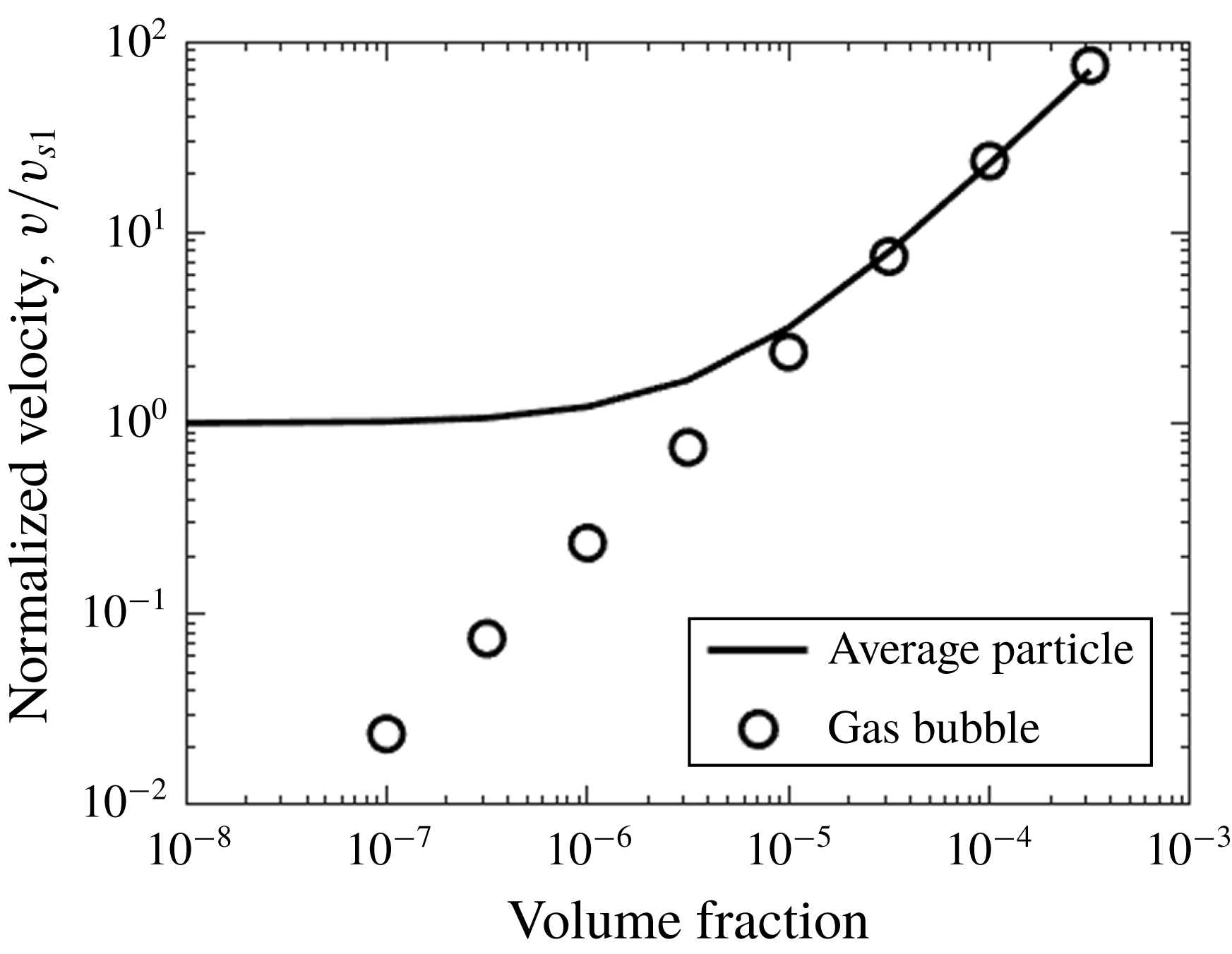
These results show that a cloud of aerosol particles can behave as a gas droplet in continuum flow even when the individual particles are small relative to the mean free path of the gas. This occurs for sufficiently large cloud sizes and particle volume fractions.
Of course, in real-world situations the cloud will not be perfectly spherical, nor will it be composed of monodisperse particles arranged in a regular grid. Nevertheless, we can reach some qualitative conclusions about the behaviour of a real-world cloud of aerosol particles from the results of the ideal case. First, the deposition velocity of the particles in the cloud may be significantly greater than the deposition velocity of an isolated particle. This enhanced settling velocity is due to the fact that the particles entrain the surrounding fluid. Second, a collection of particles that behave as if they are in the transition flow regime when they are isolated (or when the volume fraction is very small) can behave like a cloud of continuum particles when the particle volume fraction increases. This is because the long-range hydrodynamic interactions between particles decay as
 $1/r$
, regardless of the size of the particle relative to the gas mean free path.
4.2 Additional considerations
Before concluding, we will address a number of assumptions that we made for our analysis. First, we have ignored rotational effects when considering interactions between particles. The complete description of two particles has the same general form as (2.1), but one replaces the 3-element velocity and force vectors with 6-element vectors that include the angular velocity of and torque exerted by the particle, respectively. Likewise, one would need to incorporate rotational effects in the generalized mobility tensors
 $\unicode[STIX]{x1D648}_{ij}$
, which now have size 6-by-6. See Brenner (Reference Brenner1967) or Carrasco & García de la Torre (Reference Carrasco and García de la Torre1999) for the effects of rotation on a single particle in the continuum and our previous work (Corson et al.
Reference Corson, Mulholland and Zachariah2017b
) for how one might consider rotational effects in the kinetic regime. The two-particle principles follow from the application of KR-based theories to single-particle systems.
Second, we have mostly ignored Brownian effects in our calculations, except to note that Brownian forces would likely randomize the orientations of aggregates in an aerosol. Strictly speaking, one must account for hydrodynamic interactions when determining the probability distribution for the particle orientation. For example, Mackaplow & Shaqfeh (Reference Mackaplow and Shaqfeh1998) have performed dynamic simulations showing non-Brownian fibres aligning with gravity due to hydrodynamic effects. Therefore, the orientation of aerosol aggregates will depend on the competition between hydrodynamic effects that tend to align particles and Brownian effects that tend to randomize their orientation. This is analogous to the behaviour of a perfectly conducting aerosol particle in an external electric field (Li, Mulholland & Zachariah Reference Li, Mulholland and Zachariah2014; Corson et al. Reference Corson, Mulholland and Zachariah2018b ).
Additionally, Brownian forces affect the spatial distribution of particles in a cloud or suspension. Diffusion is partially responsible (along with shear) for break-up of clouds (Fuchs Reference Fuchs1964), so the analysis in the previous section applies only for some initial period while the cloud remains intact. For statistically homogeneous systems, one must account for the particle probability distribution when determining suspension behaviour. In principle, one can apply the methods used in Stokesian dynamics simulations (see e.g. Ermak & McCammon (Reference Ermak and McCammon1978) and Brady & Bossis (Reference Brady and Bossis1988)) for non-continuum flows, provided one modifies the hydrodynamic interaction terms in the algorithms. We have provided here the translational hydrodynamic interaction tensors, while we describe how to account for rotational and translation–rotation coupling effects elsewhere (Corson et al. Reference Corson, Mulholland and Zachariah2017b ).
Third, our calculations have been performed for isothermal conditions. As Fuchs notes, cloud behaviour is often driven by temperature differences between the cloud interior and the surrounding gas (Fuchs Reference Fuchs1964). Because aerosols are often generated in non-isothermal systems (e.g. flames), one must take care in applying our analysis to real-world systems.
Finally, our calculations assume the particles are in an unbounded, non-periodic system. Note that in periodic, statistically homogeneous suspensions, the sedimentation velocity decreases with increasing particle volume fraction (Batchelor Reference Batchelor1972). In contrast, unbounded clouds of particles settle at a faster rate as volume fraction increases, as is clear from (4.4). The difference is due to the gas behaviour: for an unbounded cloud, the gas can flow around the cloud to occupy the space vacated by the settling cloud, whereas the gas must flow between the particles in the opposite direction of the sedimentation velocity. This counter-flow serves to reduce the sedimentation velocity of the periodic suspension.
5 Conclusions
We have described how one would apply our extended Kirkwood–Riseman theory to interactions between spheres and aggregate particles as a function of the distance between particles and the particle size and shape (number of spheres, primary sphere Knudsen number, fractal dimension). We have provided sample results for the effects of hydrodynamic interactions between two spheres and two aggregates in the transition regime. In both cases, the interactions are weaker than for particles in continuum flow, and the interaction strength decreases with increasing Knudsen number. We note that in many aerosols of engineering interest, the particle volume fraction is very small, so hydrodynamic interactions may have little impact on measurable quantities such as viscosity and sedimentation rates. However, for aerosols near the gel point, such interactions may be important. It is also possible that hydrodynamic interactions have a noticeable impact on coagulation rates even for dilute systems, though we have not explored this issue as part of the current study.
We have also developed a point force method for particles (aggregates or spheres) in the transition regime. Our results demonstrate point force method is in good agreement with our EKR method at moderate and large separation distances. This method greatly simplifies the analysis of systems consisting of multiple aggregates by replacing each aggregate with an equivalent particle, which reduces the number of equations one must solve simultaneously from three times the total number of spheres in all the aggregates to three times the number of aggregates (for three-dimensional systems).
We have applied our point force method to an unbounded cloud of spheres with non-negligible Knudsen numbers and shown that it behaves similarly to a cloud of larger particles. This analysis applies to an isothermal, spherical cloud of particles arranged in a regular grid, but the conclusion that hydrodynamic interactions among a large group of particles can significantly affect settling behaviour also applies in less restrictive conditions.
The above work provides some of the hydrodynamic interaction terms necessary to perform a Brownian dynamics simulation of an aerosol consisting of particles with non-negligible Knudsen numbers. One could either apply the point force method described here or our more complicated EKR method to account for Brownian (through the generalized Stokes–Einstein relation; see Ermak & McCammon (Reference Ermak and McCammon1978)) and hydrodynamic effects on the aerosol behaviour. One can also account for rotational effects using the EKR method, as discussed elsewhere (Corson et al. Reference Corson, Mulholland and Zachariah2017b ). Taken together, this work can form the basis for a dynamic simulation of an aerosol system consisting of particles in the transition regime.