2.1 Self-similar motion of turbulent vortex rings

The structure of self-similar turbulent vortex rings is determined in the framework of the semi-empirical theory of turbulence using the turbulent eddy viscosity in the momentum balance equation

supplemented with the continuity equation for the incompressible mean flow

where bold characters denote vectors, $\boldsymbol{v}$ is the average flow velocity, $\boldsymbol{F}$ represents the body force, $t$ is time, $\unicode[STIX]{x1D70C}$ is the fluid density, $p$ is the pressure and $\unicode[STIX]{x1D708}$ is the turbulent eddy viscosity, $\unicode[STIX]{x1D708}(t)=\unicode[STIX]{x1D706}W(t)R(t)$ , in which $\unicode[STIX]{x1D706}$ is an empirical constant, $W$ is the axial velocity of the vortex ring and $R$ is its radius.

The vortex ring is assumed to be axisymmetric on average. Then, the cylindrical coordinate system shown in figure 1 (from the $z{-}r$ coordinate origin) is introduced, with the $z$ -coordinate being reckoned along the ring axis and the $r$ -coordinate in the radial direction. The vorticity, $\unicode[STIX]{x1D734}=\unicode[STIX]{x1D735}\times \boldsymbol{v}$ , has only the azimuthal component, which is denoted as $\unicode[STIX]{x1D6FA}$ . The velocity components are generated by the streamfunction $\unicode[STIX]{x1D713}$ , as $v_{z}=r^{-1}\unicode[STIX]{x2202}\unicode[STIX]{x1D713}/\unicode[STIX]{x2202}r$ and $v_{r}=-r^{-1}\unicode[STIX]{x2202}\unicode[STIX]{x1D713}/\unicode[STIX]{x2202}z$ (Loitsyanskii Reference Loitsyanskii1966), which satisfy (2.2). Then, equation (2.1) takes the form of the modified Helmholtz equation,

while the definition of vorticity yields

Figure 1.

Schematic of the coordinate systems used for the description of the turbulent vortex ring of propellant gases moving towards the target and of the backward spatter of blood. The cylindrical coordinates $r$ and $z$ are associated with the radial and axial directions of the turbulent vortex ring and its origin is at the muzzle of the gun. The Cartesian coordinate system X–Y–H is used for the description of the trajectories of blood droplets in backward spatter resulting from a bullet impacting the target (the blood source).

The hydrodynamic vortex impulse is defined as

where the integration is performed over an unbounded volume. The vortex impulse $\boldsymbol{P}$ is the integral invariant of the equations of motion, equations (2.3) and (2.4) (Alekseenko, Kuibin & Okulov Reference Alekseenko, Kuibin and Okulov2007; Akhmetov Reference Akhmetov2009). Therefore, the impulse can be fully determined by the initial vorticity distribution in the turbulent vortex ring $\unicode[STIX]{x1D6FA}_{0}(r,z)$ ,

where subscript zero indicates the initial value.

It should be emphasized that the unbound geometry in the integral in (2.6) is a good approximation, because the confinement sizes are typically much larger than the sizes of such turbulent vortex rings. This situation is essentially similar to that of the Schlichting submerged jet, or any other self-similar laminar and turbulent jets, for which analytical solutions are known from the boundary layer theory (Schlichting Reference Schlichting1979; Yarin Reference Yarin, Tropea, Yarin and Foss2007). Only when a normal head-on collision of a vortex ring onto a wall is considered, could the effect of the wall on the ring be pronounced, but only at distances from the wall of the order of the cross-sectional radius of an effective vortex-ring core. Obviously, if the original gunshot happens in direct contact with an obstacle, vortex rings do not form, and the blood droplets could be affected by other near-field details of the muzzle gas flow field such as the Prandtl–Meyer expansion fan.

It should be emphasized that the initial radius of the turbulent vortex ring is comparable to the radius of the muzzle exit and much smaller than the radius of the turbulent vortex ring as it propagates towards the target. Therefore, the initial radius can be neglected, the idealization that makes the problem self-similar (Yarin Reference Yarin, Tropea, Yarin and Foss2007). Then, the dimensionless self-similar coordinates, $\overline{r}$ and $\overline{z}$ , are introduced, as well as other functions, following standard considerations of the theory of self-similar flows (Lugovtsov Reference Lugovtsov1974; Yarin & Weiss Reference Yarin and Weiss1995)

where $\unicode[STIX]{x1D706}_{0}$ is a dimensionless empirical constant.

Accordingly, equations (2.3) and (2.4) take the following dimensionless self-similar forms:

The solutions of (2.8) and (2.9) are subject to the boundary conditions

and should satisfy the following integral invariant condition associated with (2.6):

Equations (2.8) and (2.9) can only be solved numerically. However, an analytical solution can be constructed when a plausible approximation of the right-hand side of (2.8) is introduced. Namely, having in mind that the axial velocity of turbulent vortex rings is typically much higher than the radial one, i.e. $v_{z}\gg v_{r}$ , and thus $\unicode[STIX]{x2202}\overline{\unicode[STIX]{x1D713}}/\unicode[STIX]{x2202}\overline{r}\gg \unicode[STIX]{x2202}\overline{\unicode[STIX]{x1D713}}/\unicode[STIX]{x2202}\overline{z}$ , equation (2.8) is approximated by the equation

where $\overline{r}_{m}$ and $\overline{z}_{m}$ are the locations of the maximum of the vorticity function $\overline{\unicode[STIX]{x1D6FA}}(\overline{r},\overline{z})$ .

The analytical solution of the system of equations (2.9) and (2.13) reads

where

The empirical coefficient $\unicode[STIX]{x1D706}_{0}$ is related to the ratio of the coordinates of the maximum vorticity locations, $\unicode[STIX]{x1D6FC}=\overline{r}_{m}/\overline{z}_{m}$ , as

It should be emphasized that the ratio $\unicode[STIX]{x1D6FC}$ can be measured experimentally, which determines the only empirical parameter of the semi-empirical theory of turbulent vortex rings, $\unicode[STIX]{x1D706}_{0}$ , through (2.19).

The solution of (2.9) and (2.13) resulting in (2.14)–(2.19) was recently published by Akhmetov (Reference Akhmetov2009) without any derivation. The original derivation given by Lugovtsov (Reference Lugovtsov1974) is difficult to obtain; therefore, its complete derivation is proven independently in this work and shown in appendix A.

2.2 Transport of gunpowder particles by a turbulent vortex ring

The transport of gunpowder particles by a turbulent vortex ring is described using the following equation:

where $c$ is the average gunpowder particle concentration in units of $\text{particles}~\text{cm}^{-3}$ , $D$ is the turbulent diffusion coefficient, and $D=\unicode[STIX]{x1D6FE}\unicode[STIX]{x1D708}$ , where $\unicode[STIX]{x1D6FE}$ is the inverse turbulent Schmidt number.

The total number of gunpowder particles is invariant and thus equation (2.20) possesses the following integral invariant:

where $N_{0}$ is the total number of gunpowder particles released from the muzzle.

Similarly to the flow field, the gunpowder particle concentration in the present case is also self-similar, and thus (2.20) takes the following self-similar form:

where

The solution of (2.22) should satisfy the following boundary conditions:

As in the momentum balance equation discussed in § 2.1, we account for the fact that $v_{z}\gg v_{r}$ , and thus $\unicode[STIX]{x2202}\overline{\unicode[STIX]{x1D713}}/\unicode[STIX]{x2202}\overline{r}\gg \unicode[STIX]{x2202}\overline{\unicode[STIX]{x1D713}}/\unicode[STIX]{x2202}\overline{z}$ , and reduce (2.22) to the following form:

Introduce the following variables to find an analytical solution of (2.26),

where $K=\left.{\overline{r}_{m}}^{-1}\unicode[STIX]{x2202}\overline{\unicode[STIX]{x1D713}}/\unicode[STIX]{x2202}\overline{r}\right|_{\substack{ \overline{r}=\overline{r}_{m} \\ \overline{z}=\overline{z}_{m}}}$ and $m=\sqrt{8\unicode[STIX]{x1D6FE}\unicode[STIX]{x1D706}_{0}}$ .

The solution is sought in the form

Accordingly, equation (2.26) yields the following equation for the function $\unicode[STIX]{x1D6E4}(\unicode[STIX]{x1D709},\unicode[STIX]{x1D702})$ :

With the factorization $\unicode[STIX]{x1D6E4}(\unicode[STIX]{x1D709},\unicode[STIX]{x1D702})=\unicode[STIX]{x1D6E4}_{1}(\unicode[STIX]{x1D709})\unicode[STIX]{x1D6E4}_{2}(\unicode[STIX]{x1D702})$ , equation (2.29) yields the following two ordinary differential equations:

where $A$ is a separation constant.

The integral invariant of (2.21) takes the following form:

Equation (2.30) is known in the theory of one-dimensional quantum oscillators and its solution satisfying equation (2.32) is readily available (Tikhonov & Samarskii Reference Tikhonov and Samarskii1990; Arfken, Weber & Harris Reference Arfken, Weber and Harris2013) as

where $B_{1}$ is a constant, $H_{j}$ are the Hermite polynomials, and $A+3=2j+1$ , where $j=0,1,2,\ldots .$

Equation (2.31) is also known in the theory of cylindrical quantum oscillators (Pauling & Wilson Reference Pauling and Wilson1935), and its solution satisfying equation (2.32) exists only when $-A=2(2i+1)$ , where $i=0,1,2,\ldots .$ Then, it is seen that the only appropriate choice is $i=j=0$ , which yields $A=-2$ , and (2.31) results in

where $B_{2}$ is a constant.

Therefore, $\unicode[STIX]{x1D6E4}(\unicode[STIX]{x1D709},\unicode[STIX]{x1D702})$ becomes

where $B$ is a constant that incorporates all the previous factors and is determined from the integral invariant, equation (2.32), as

Then, equations (2.28), (2.35) and (2.36) result in

Through the variable transformation in (2.27), the latter equation yields the solution for the concentration of gunpowder particles transported by a turbulent vortex ring in the following form:

2.3 Deflection of blood droplets in backward spatter by the turbulent vortex ring

When a bullet impacts a target and blood is splashed in the direction opposite to bullet motion (i.e. backward spatter), the turbulent vortex ring of propellant gases following the bullet can encounter the airborne blood droplets moving in the opposite direction. These blood droplets form due to the Rayleigh–Taylor instability which occurs in backward spatter because the denser blood is accelerated towards air (Chandrasekhar Reference Chandrasekhar1981; Comiskey et al. Reference Comiskey, Yarin, Kim and Attinger2016, Reference Comiskey, Yarin and Attinger2017b ). The theory of this instability has been used to predict the formation of blood droplets in two different cases of backward spatter, by sharp and blunt bullets, in Comiskey et al. (Reference Comiskey, Yarin, Kim and Attinger2016) and Comiskey et al. (Reference Comiskey, Yarin and Attinger2017b ). In the latter works, backward spatter is considered as a system of two interpenetrating continua, with a blob of blood droplets propagating through air experiencing aerodynamic drag, producing viscous suction and causing air entrainment. The leading blood droplets experience the highest drag and entrain air in their wake, which reduces the air drag experienced by the following droplets. This collective effect, resembling a flock of geese flying in V-formation, allows the droplets to fly further (Murzabayev & Yarin Reference Murzabayev and Yarin1985).

Following the work of Comiskey et al. (Reference Comiskey, Yarin, Kim and Attinger2016), the drag force acting on a droplet along its trajectory, $\boldsymbol{F}_{D,i}$ , with entrained air is

where $l_{\ast ,i}$ is an individual droplet diameter determined by the Rayleigh–Taylor instability (Comiskey et al. Reference Comiskey, Yarin, Kim and Attinger2016, Reference Comiskey, Yarin and Attinger2017b ), $C_{D,i}$ is the drag coefficient, $\unicode[STIX]{x1D70C}_{a}$ is the density of air, $\boldsymbol{u}_{i}$ is the instantaneous averaged velocity of the blood droplets in a blob (bin) $i$ along the droplet trajectory, and $\boldsymbol{U}_{i}$ is the instantaneous averaged velocity of entrained air in the blob along the trajectory.

The momentum balance of blood droplets in a blob with air entrainment is then

where $M_{i}$ is the mass of blood in the blob, $T$ is the time reckoned from the moment these droplets have been spattered, $n_{i}$ is the number of blood droplets in the blob, $\unicode[STIX]{x1D749}$ is the unit vector tangential to the trajectory, and $\boldsymbol{i}$ , $\boldsymbol{j}$ and $\boldsymbol{k}$ are the unit vectors of the X–Y–H axes shown in figure 1. Note that a temporal offset exists between the formation of the turbulent vortex ring and the backward spatter of blood droplets. Therefore, the time $t$ , in which the evolution and propagation of the turbulent vortex ring is tracked, and the time $T$ , in which droplet motion is calculated, are related as

where $V_{A}$ is the velocity of the bullet approaching the target, and $\unicode[STIX]{x1D6FF}$ is the distance between the muzzle exit and the target (cf. figure 1).

If the airborne blood droplet blob encounters a turbulent vortex ring, the counter-flow of air generated by the latter sheds the air cloud entrained by the blob, i.e. the velocity and volume of the entrained air, $U_{i}\rightarrow 0$ and $V\rightarrow 0$ , respectively (cf. appendix B). Then, the drag force acting on a droplet blob becomes associated with the velocity of the counter-flow generated by the turbulent vortex ring as

where $\boldsymbol{v}$ is the velocity vector of the turbulent vortex ring. It should be emphasized that (2.42) does not include the effect of the air entrained by flying droplets before the strong interaction with the oncoming vortex ring has begun because the entrained air is easily shed back by the ring long before the droplets are affected by the collision.

The momentum balance of blood droplets in a blob interacting with a turbulent vortex ring is expressed as

The projection of (2.40) and (2.43) on the X–Y–H axes and the appropriate initial conditions are described in appendix B.

In the case of a strong interaction of the blood droplet blob and the turbulent vortex ring, the blood droplet velocity $u_{i}$ will slow down to zero. Then, droplet motion along the trajectory will cease, and the droplet blob will be pushed by the turbulent vortex ring in the opposite direction. The interaction of the turbulent vortex ring and a turned-around blood droplet blob is relatively short because the turbulent vortex ring propagates rapidly, and its velocity field is practically not felt outside of the vortex body. Then, the droplet blob will continue moving towards the target, entraining the surrounding air once again according to the mechanisms described in (2.40). Also, the droplet blobs that passed through the vortex ring will continue moving from the target, entraining the surrounding air once again according to the mechanisms described in (2.40).

Figure 2.

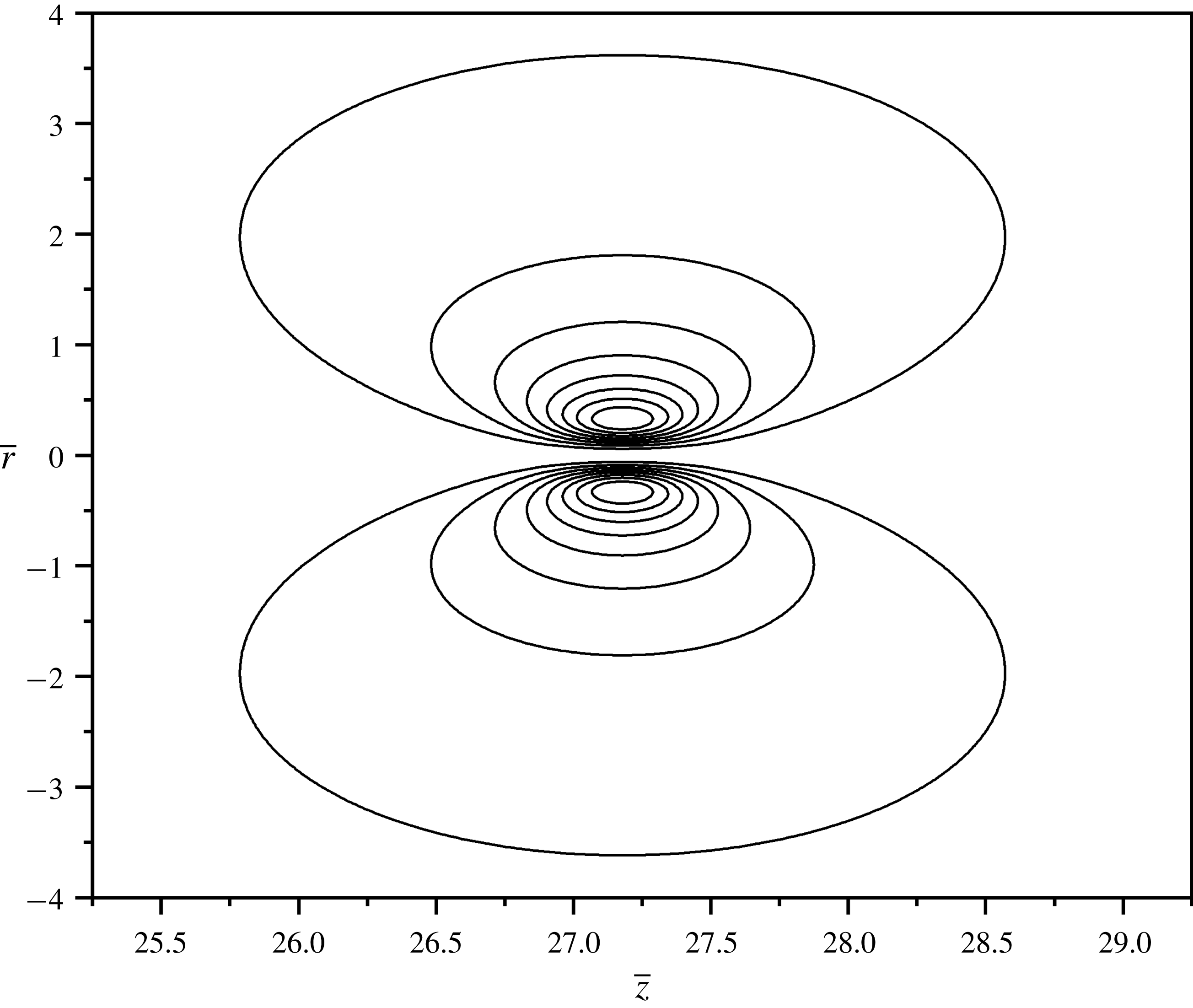
Self-similar streamlines of the turbulent vortex ring with $\unicode[STIX]{x1D6FC}=5.5\times 10^{-3}$ ( $\unicode[STIX]{x1D706}_{0}=4.4\times 10^{-3}$ ). The values of the streamlines from the outward line going inwards are 0.022–0.176 in steps of 0.022.

3.1 Propagation of propellant gases

The dimensionless empirical parameter $\unicode[STIX]{x1D706}_{0}$ involved in the semi-empirical theory of turbulent vortices is found using (2.19) and data for the coordinates of the locations of the maximum vorticity, $\unicode[STIX]{x1D6FC}=\overline{r}_{m}/\overline{z}_{m}$ . The latter was found experimentally as $\unicode[STIX]{x1D6FC}\approx 10^{-3}{-}10^{-2}$ (Maxworthy Reference Maxworthy1974; Akhmetov Reference Akhmetov2009). For the value of $\unicode[STIX]{x1D6FC}=5.5\times 10^{-3}$ , which corresponds to the value of $\unicode[STIX]{x1D706}_{0}=4.4\times 10^{-3}$ , the field of the self-similar streamfunction found from (2.14) is shown in figure 2. Note that, unless otherwise specified, this value of $\unicode[STIX]{x1D6FC}$ , and thus $\unicode[STIX]{x1D706}_{0}$ , is used hereinafter in this work. The vorticity of such a turbulent vortex ring was reported to be highly localized (Sullivan, Widnall & Ezekiel Reference Sullivan, Widnall and Ezekiel1973), which is corroborated in figure 3, plotted using (2.15).

Figure 3.

Self-similar vorticity field of the turbulent vortex ring with $\unicode[STIX]{x1D6FC}=5.5\times 10^{-3}$ ( $\unicode[STIX]{x1D706}_{0}=4.4\times 10^{-3}$ ).

The field of the self-similar concentration of gunpowder particles found from (2.38) with $\unicode[STIX]{x1D6FE}=1$ (corresponding to a turbulent Schmidt number equal to one, a plausible approximation for turbulent flows (Yarin Reference Yarin, Tropea, Yarin and Foss2007)) is shown in figure 4.

Figure 4.

Field of the self-similar concentration of gunpowder particles in the turbulent vortex ring with $\unicode[STIX]{x1D6FC}=5.5\times 10^{-3}$ ( $\unicode[STIX]{x1D706}_{0}=4.4\times 10^{-3}$ ) and $\unicode[STIX]{x1D6FE}=1$ .

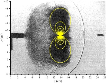
Using the self-similar solution, the time-dependent flow pattern can be reconstructed using (2.7), and the resultant flow field can be overlaid on experimental images of muzzle gases. Such data are available in Klingenberg & Heimerl (Reference Klingenberg and Heimerl1992) where a 5.56 mm calibre M-16 rifle firing ball ammunition was photographed during the early development of the muzzle flow pattern close to the muzzle of the rifle. There were four photographs taken at 10, 37, 105 and $237~\unicode[STIX]{x03BC}\text{s}$ after the bullet left the muzzle, and the final image at $237~\unicode[STIX]{x03BC}\text{s}$ shows a plume of muzzle gases and the turbulent vortex ring. The theoretical flow pattern predicted using (2.14) overlaid on this experimental image is shown in figure 5. Note that other structures inherent to the propagation of muzzle gases (such as the precursor blast wave) discussed in § 1 are also seen in figure 5. The impulse of the vortex ring was found by fitting its position to the experimental image, which yields $P_{0}=75~\text{cm}^{4}~\text{s}^{-1}$ . The corresponding streamlines predicted with the values of $\unicode[STIX]{x1D6FC}$ (and thus $\unicode[STIX]{x1D706}_{0}$ ) and $P_{0}$ mentioned above properly fit the dark area in figure 5.

Figure 5.

Theoretically predicted flow pattern in the turbulent vortex ring at $237~\unicode[STIX]{x03BC}\text{s}$ after the bullet left the muzzle of the gun. The experimental image is taken from Klingenberg & Heimerl (Reference Klingenberg and Heimerl1992). The values of the streamfunction corresponding to the streamlines from the outward line to the inward one are $\unicode[STIX]{x1D713}=0.8{-}37.4~\text{cm}^{3}~\text{s}^{-1}$ in steps of $0.8~\text{cm}^{3}~\text{s}^{-1}$ .

The propagation of the turbulent vortex ring can be followed by the locations of the maximum vorticity versus time, which are found from (2.7), (2.17) and (2.18) as

For the turbulent vortex ring shown in figure 5, the values of $\overline{z}_{m}=27.18$ and $\overline{r}_{m}=0.1495$ (corresponding to $\unicode[STIX]{x1D6FC}=5.5\times 10^{-3}$ , and thus $\unicode[STIX]{x1D706}_{0}=4.4\times 10^{-3}$ ), with $P_{0}=75~\text{cm}^{4}~\text{s}^{-1}$ , yield the axial and radial positions of the maximum vorticity through (3.1), as is shown in figure 6.

Figure 6.

Location of the maximum vorticity in the turbulent vortex ring of the propellant gases over time: (a) the axial position, (b) the radial position.

The concentration of gunpowder particles swept by a turbulent vortex ring depends on the total number of particles within the cartridge, $N_{0}$ . This value can be evaluated knowing the volume of a single gunpowder particle and the volume of the cartridge, which holds all the gunpowder particles. For spherical gunpowder particles of 1 mm diameter (Brown Reference Brown1998), and the volume of the cartridge of approximately 1 ml, one finds the number of particles as $N_{0}\approx 1500~\text{particles}$ . It should be emphasized that $N_{0}$ is not the number of particles that crime scene investigators may find at the location of a violent crime as a result of a gunshot; but rather it is the approximate number of gunpowder particles within the cartridge. The concentration of gunpowder particles (as a function of time) swept by the turbulent vortex ring of propellant gases with an impulse in the $P_{0}=50{-}125~\text{cm}^{4}~\text{s}^{-1}$ range (which incorporates the value of $P_{0}=75~\text{cm}^{4}~\text{s}^{-1}$ established above), is shown in figure 7. Note that the chosen impulse range is intended to encompass slight deviations between manufacturers for the same calibre bullet and firearm type. The impulse value is fundamentally dependent upon the physicochemical processes relevant for propellant powder, which, to an extent, are determined by the bullet and cartridge type. The concentration is calculated using (2.23) and (2.38), and the order of magnitude of the concentration is within the realm of what was observed experimentally, as Klingenberg & Heimerl (Reference Klingenberg and Heimerl1992) reported $10^{5}{-}10^{8}~\text{particles}~\text{cm}^{-3}$ .

Figure 7.

Gunpowder concentration in the turbulent vortex ring of propellant gases for $N_{0}=1500~\text{particles}$ and the range of $P_{0}$ indicated in the legend. The units for $P_{0}$ are $\text{cm}^{4}~\text{s}^{-1}$ .

3.2 Effect of the propellant gases on the backward spatter of blood

To study the effect of a turbulent vortex ring of propellant gases on the backward spatter of blood droplets, the case of a blunt bullet impacting a target normally from 30 cm is considered with the same set of parameters as in Comiskey et al. (Reference Comiskey, Yarin and Attinger2017b ). Namely, the blood spatter splash angle is $\unicode[STIX]{x0394}\unicode[STIX]{x1D703}=15^{\circ }$ , the approaching bullet velocity is $V_{A}=1000~\text{m}~\text{s}^{-1}$ , and the droplet size $l_{\ast ,i}$ ranges from ${\sim}0.2$ to 0.4 mm, which is the size range present in backward blood spatter due to a gunshot Comiskey et al. (Reference Comiskey, Yarin, Kim and Attinger2016). The initial height (the droplet origin) was set to be $H_{0}=100~\text{cm}$ . The equations of Comiskey et al. (Reference Comiskey, Yarin, Kim and Attinger2016, Reference Comiskey, Yarin and Attinger2017b ) for the droplet trajectory calculations were modified to incorporate an interaction with the turbulent vortex ring affecting the aerodynamic drag force, as described in § 2.3. In order to reveal the effect of the impulse of the turbulent vortex ring, $P_{0}$ , it was varied from 75 to $150~\text{cm}^{4}~\text{s}^{-1}$ , and the final locations on the floor of several bins of blood droplets predicted with and without accounting for the interaction with a turbulent vortex ring are shown in figure 8.

Figure 8.

Final blood droplet bin locations on the floor accounting for an interaction with and without a turbulent vortex ring. The impulse of the vortex ring is (a)  $P_{0}=75~\text{cm}^{4}~\text{s}^{-1}$ and (b)  $P_{0}=150~\text{cm}^{4}~\text{s}^{-1}$ . The red circles and grey squares represent the cases with and without the interaction with the turbulent vortex ring, respectively.

When the interaction with the turbulent vortex ring is accounted for, the blood droplet bins can be deflected further from the target than without such interactions, as seen in figure 8(b), for example. On the contrary, the blood droplet bins can be overcome by the turbulent vortex ring and turn towards the target. These bins can either be deflected and spread outwards (in the Y-direction, as shown in figure 8), or hit the target as indicated by the large quantity of red circles located around $X=0$ in figure 8. The predicted spatial distributions of the number of stains and the average stain area presented in the form of histograms binned every 20 cm from the target are shown in figures 9 and 10, respectively.

Figure 9.

Spatial distribution of the number of bloodstains from a gunshot formed on the floor by backward spatter. (a) The case of a turbulent vortex ring with the impulse of $P_{0}=75~\text{cm}^{4}~\text{s}^{-1}$ , and (b) with the impulse of $P_{0}=150~\text{cm}^{4}~\text{s}^{-1}$ . The grey bars indicate the distributions predicted without an interaction with the vortex ring, and the red bars are for the case where the interaction was accounted for.

Figure 10.

Spatial distribution of the average stain area from a gunshot formed on the floor by backward spatter. (a) The case of a turbulent vortex ring with the impulse of $P_{0}=75~\text{cm}^{4}~\text{s}^{-1}$ , and (b) with the impulse of $P_{0}=150~\text{cm}^{4}~\text{s}^{-1}$ . As in figure 9, the grey bars indicate the distributions predicted without an interaction with the vortex ring, and the red bars are for the case where the interaction was accounted for.

The interactions with the turbulent vortex rings result in significant changes in the final locations of the bloodstains on the floor and their average areas. For the impulse of $P_{0}=75~\text{cm}^{4}~\text{s}^{-1}$ , 18 % of the droplets splashed fall on the floor within 20 cm of the target, whereas for the impulse of $P_{0}=150~\text{cm}^{4}~\text{s}^{-1}$ , 41 % of the droplets splashed fall within that range. A higher value of the vortex impulse is equivalent to a closer shooting distance (for self-similar vortex rings). Accordingly, these results show that a closer shooting distance results in more blood droplets turning around and travelling towards the target. This effect is important for crime scene investigation, and its prediction here can serve as a guidance for a future experimental work. Note also that these exploratory results should be correlated with a separate parametric study of the flow field of propellant gases for a variety of common firearms.