NOMENCLATURE
Abbreviation
- CFD
Computational Fluid Dynamics
- CFL
Courant-Friedrichs-Lewy
- PDPA
Phase Doppler Particle Analyzer
- PIV
Particle Image Velocimetry
- IW
Interrogation Window
- ROI
Region of Interest
- A
Area of cross-section,
 ${{\rm{m}}^2}$
-
${C_p}$
Specific heat at constant pressure, J/kgK
- d
Fuel injector diameter, m
- D
Cavity depth, m
- F
Fuel-air mass ratio
-
${f_s}$
Stoichiometric fuel/air ratio
- h
Fuel jet penetration height, m
- H
Pylon height, m
- L
Cavity length, m
- M
Mach number
-
$\dot m$
Mass flow, kg/s
- MW
Molecular weight, g/mol
- P
Static pressure, N/
${{\rm{m}}^2}$
-
${P_T}$
Total pressure, N/
${{\rm{m}}^2}$
- R
Universal gas constant, J/kmol.K
- T
Static temperature, K
- U
Streamwise velocity, m/s
- x,y,z
Cartesian coordinates


Subscripts
- atm
Atmospheric
- w
Wall
- k
Species
Greek Symbol
-
$\alpha $
Fuel mass fraction
-
${\eta _m}$
Mixing effectiveness
-
$\Lambda $
Total pressure loss
-
$\lambda $
Thermal conductivity, W/mK
-
$\rho $
Density, kg/
${{\rm{m}}^3}$
- µ
Viscosity, kg/ms


1.0 INTRODUCTION
The study of supersonic combustion has been an active research area in the aerospace propulsion domain. Though the simplicity and efficiency at high Mach numbers make the scramjet concept interesting, the combustion part of the engine has difficulties in attaining ignition and sustaining combustion at high-speed gas flows. The supersonic air stream within the combustion chamber reduces the residence time and therefore results in poor mixing efficiency of the air-fuel mixture. Over the years, researchers have tried various concepts in fuel injection and combustor geometries to achieve a stable flame holding capability as well as enhanced mixing. Commonly used concepts are instream injection and wall-based injection(Reference Gerlinger, Stoll, Kindler, Schneider and Aigner1–Reference Huang4). These concepts help to create recirculation regions of fuel and oxidisers which thereby increase the residence time to mix and reside long enough to get ignited and burned(Reference Bogdanoff5–Reference Quan Li, Huang, Yan, Tao Zhao and Liao8).
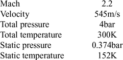
Inlet conditions for the combustor

Instream injection is performed with the help of a strut geometry, which is located at the central axis of the combustor. This helps in injecting the fuel into the combustor core directly and thereby achieving sufficient mixing and fuel jet penetration. However, there exists a huge pressure loss as a trade-off. This led to the concept of wall-based injection such as cavities, ramps and angled combustor walls(Reference Huang9,Reference Gruber, Donbar, Carter and Hsu10) . The use of these geometrical features helps in creating a recirculation region within the combustor thereby increasing the residence time of the air so that a sufficient amount of time will be available to get well mixed with the fuel stream. Unlike instream injection, there are no large geometries present in wall-based injection resulting in minimal total pressure loss. The wall-based injection also has few trade-offs. The presence of a supersonic crossflow over the cavity restricts the fuel penetration and, therefore, the jet penetration height is very low. One possible solution is to introduce a pylon geometry at the leading-edge of the cavity. The pressure difference between the cavity floor and pylon helps in improving the mass flow exchange between cavity flow and crossflow along with the fuel jet penetration capability(Reference Freeborn, King and Gruber11). The fluid that moves upward travels between a pair of counter-rotating vortices generated by the pylon which enhances mixing(Reference Bao, Zhou and Pan12). Though there are various studies based on pylon-cavity geometries, the information on fundamental mixing mechanisms is limited.
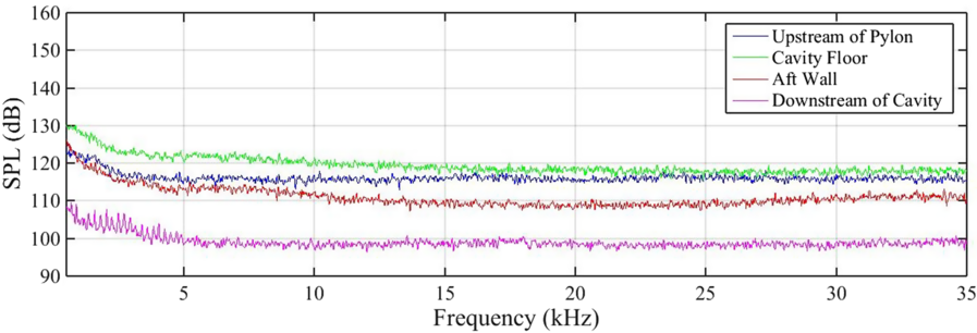
In the current study the effect of variations in pylon geometry on performance parameters such as flammable plume area, fuel jet penetration, mixing efficiency, total pressure loss and streamwise vorticity are investigated for a combustor inlet Mach number of 2.2 which approximates a flight Mach number of 5, at a total pressure of 4bar and total temperature of 300K(Reference Doster13,Reference Freeborn14) . The temperature of the current study does not represent the actual flight condition due to the inability of the freejet facility to control the temperature. In reality, the static temperature entering the combustor would exceed 600K. The expected test section inlet conditions for the current study are given in Table 1. Based on the available literature, an optimum length to depth (L/D) ratio of 3 and an aft wall angle of 45° for the cavity is selected to minimise the form drag and acoustic oscillations(Reference Ren, Wang, Hu and Zheng15–Reference Zhang and Edwards17). Figure 1 shows the power spectra in the form of Sound Pressure Level (SPL) vs frequency for the pressure transducers located at various locations where there is no occurrence of discrete large magnitude peaks is observed. Basic geometric features of the pylon such as height, width and length are kept constant. A common fuel injection location has opted for all the cases.
FFT plots of cavity oscillations for the pylon-cavity configuration.

2.0 METHODOLOGY
An experimental and computational approach has been followed in this study. Experimental data are obtained for the validation of the numerical simulation method used, whereas the mixing studies are solely conducted based on numerical simulations.
2.1 Experimental approach
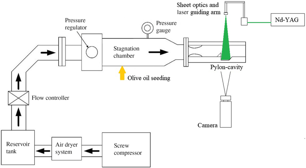
The freejet facility at the Indian Institute of Space Science and Technology (IIST), Trivandrum is used for conducting cold flow experiments. Figure 2 shows the schematic for the test facility.
Schematic for the freejet facility.

The system can provide a maximum mass flow rate of 0.6kg/s at a stagnation pressure of 4bar absolute and a stagnation temperature of 300K. The pylon-cavity baseline configuration (without injection) is mounted in an optically accessible constant area test section of 25.4mm x 25.4mm cross-section. Inlet Mach number of 2.2 is maintained using a 2D convergent-divergent nozzle, which is designed using the method of characteristics (MoC).
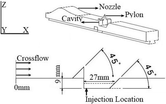
Baseline configuration that shown in Fig. 3, in this case without injection, is used for obtaining experimental data for the validation of the CFD simulation method. A pyramidal shaped pylon with smooth surfaces is selected for the baseline configuration. The baseline pylon used is of height 10mm, length 10mm, width (maximum) 5mm and a leading-edge angle of 45° which is located at the leading edge of the cavity.
Schematic for the baseline configuration (with injection for CFD simulations and without injection for experimental studies).

2.1.1 Diagnostic methods
Experimental studies include probe measurement techniques as well as laser and optical diagnostic methods.
Steady wall pressure data acquisition is performed using National Instruments PXIe-1075 Chassis, USB 6211 and OMEGA PX-309-030AV pressure transducers (accuracy: ±0:25% BSL, max) that are flush mounted along the axis of the test section floor. The precision uncertainty is calculated using the repeatability of the results for three trial runs. Approximately 0.007 bar standard deviation $\;\sigma $
, is observed for the measurements. This is converted to a 95% confidence level uncertainty as ±2
 $\sigma $
. Using the root of the sum of the squares (RSS), a total uncertainty of about ±0.017 is obtained.
Instantaneous Schlieren images are taken at 8000 fps (250µs exposure) using Phantom UHS (1280×800 pixels) with a Nikon 105mm f/2.8 macro lens and a LED light source, to visualise various quasi-steady shocks and flow features which helps in better understanding of the flow dynamics.
Particle image velocimetry (PIV) data acquisition and post-processing are done using LaVision system. A double-pulsed 532nm Nd: YAG laser from Quantel laser (Evergreen series) with a maximum pulse energy of 256 ${\rm{mJ}}$
at 10 Hz is used to create the laser sheet for the visualisation. Sheet optics and laser guiding arm from LaVision is used to obtain required laser sheet thickness of 1mm and orientation respectively. For the present test conditions, the double pulses used are of energy 35
 ${\rm{mJ}}$
and are separated with a dt of 0.12µs. This can provide the minimum acceptable particle shift of 5 pixels within the interrogation window for the velocity vector calculation. Images are captured using Imager Pro X camera of 14 bit with a Nikon 105mm f/2.8 macro lens mounted on it. To achieve a narrow depth of field, the aperture of the lens is kept at maximum (f/2.8). Both laser and camera are synchronised using a programmable timing unit (PTU) in double frame mode. Data acquisition and processing are controlled using DaVis software.
There are various sources of uncertainties that can be expected during PIV data acquisition and processing from the equipment used, particle dynamics, sampling, and image analysis(Reference Lazar, Deblauw, Glumac, Dutton and Elliott18). Among them, the ability of the seeder particles to track the main flow is the most crucial one. As a result, seeding particle selection plays a vital role in PIV measurement. Previous studies on PIV in supersonic flows showed that the particles with diameters less than 1 $\;{\rm{\mu m}}$
can give agreeable results(Reference Melling19). In the present study, the validation of the PIV data is performed using the CFD simulations, which is already validated through experimental wall pressure data. The particle diameter distribution for the olive oil seeder used for the present study is obtained using Phase Doppler Particle Analyser (PDPA). It is found that about 85% of the particles are around 0.7
 ${\rm{\mu m}}$
in diameter.
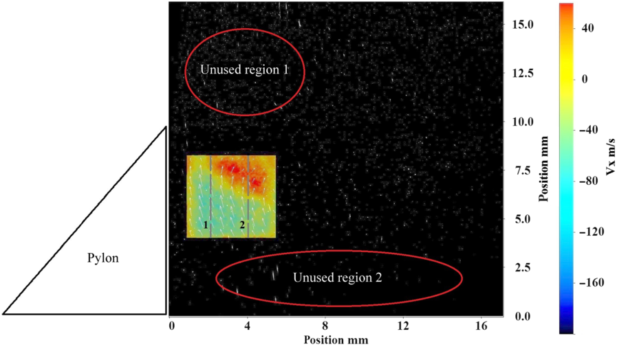
The present study investigates the instantaneous velocity distribution over the vertical mid-plane along the axis within the pylon-cavity wake region where the flowfield becomes subsonic. Figure 4 shows the region of interest (ROI) and the unusable regions for the vector calculation. The unusable region 1 consists of highly turbulent flow due to the pylon shock interaction. The frequency of fluctuations due to the shock presence cannot be captured by the current particle diameter. The region 2 is unusable due to lack of sufficient particles visible for the vector calculation. Surface wall reflections and shear layer oscillations make the particles in the region 2 difficult to detect. Current ROI for the vector calculation consists of 17673 vectors among which 265 (1.5%) vectors are rejected during processing. PIV data extracted along the two vertical dashed lines 1 and 2 shown in the figure are used for the validation of numerical data.
Average X-velocity distribution within the ROI overlapped with the experimental image frame. The regions marked red are unusable for vector estimation with the current experimental settings. The axial velocity profiles along the dashed vertical lines 1 and 2 are used for the CFD validation purposes.

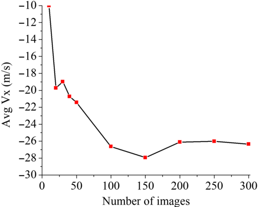
The statistical average of instantaneous X-velocity for each pair of images shows that a minimum of 200 image pairs is required to capture complete fluctuations in the flowfield (see Fig. 5).
Statistical average of Vx for a different number of image pairs.

2.2 Computational approach
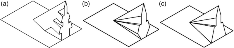
Numerical simulations are performed using the commercial solver CFD++, to investigate the effect of various pylon geometries (see Fig. 6) and the baseline geometry on mixing performance. A common transverse sonic hydrogen fuel injection from a 1mm diameter hole located at 2mm downstream of the pylon rear face has opted for the numerical study (see Fig. 3). The fundamental geometric features of the pylon such as the height of 10mm, a width of 5mm (maximum) and length of 10mm are kept constant for all the cases along with the geometrical features of the pylon-cavity baseline configuration. All three pylon geometries under investigation are shown in Fig. 6 are designed based on reducing effective blockage area and variations in vortex generating surfaces. This is to understand the resulting changes in flow features and their influence on performance parameters. The Pylon 1 geometry is designed to study the effect of reduction in effective blockage area on performance parameters. Since the formation of vortices are influenced by the slanted surfaces of the pylon, the Pylon 2 geometry is designed to accommodate additional slanted surfaces while maintaining a reduced effective blockage area. The geometry consists of both inward and outward slated surfaces. The Pylon 3 geometry is designed to understand the influence of inward and outward slanted surfaces given in Pylon 2 by keeping only the outward slanted surface of the pylon.
(a) Pylon 1 (b) Pylon 2 (c) Pylon 3.

2.2.1 Numerical scheme
Steady state computational data is obtained using compressed real gas Reynolds-averaged Navier-Stokes (RANS) equations, solved by coupled, implicit, second-order upwind solver. The ability of the RANS model to resolve the flow field for similar cases has been proven already in previous studies(Reference Huang, Li and Yan20,Reference Huang21) . CFD++ provides the Harten-Laxvan Leer-Contact (HLLC) scheme to solve the cell fluxes. For simulating the multi-species problem, the following transport equations are solved in three-dimensional Cartesian coordinates(Reference Kuo22):
a) Mass conservation
(1)
\begin{equation}\frac{{\partial \rho }}{{\partial t}} + \frac{{\partial\!\left( {\rho {u_i}} \right)}}{{\partial {x_i}}} = 0\end{equation}
b) Momentum conservation
(2)where,
\begin{equation}\frac{{\partial\!\left( {\rho {u_i}} \right)}}{{\partial t}} + \frac{{\partial\!\left( {\rho {u_i}{u_j}} \right)}}{{\partial {x_i}}} = \frac{{\partial p}}{{\partial {x_i}}} + \frac{{\partial {\tau _{ij}}}}{{\partial {x_i}}}\end{equation}
$${\tau _{ij}} = \mu \left( {\frac{{\partial {u_i}}}{{\partial {x_j}}} + \frac{{\partial {u_j}}}{{\partial {x_i}}} - \frac{2}{3}{\delta _{ij}}\frac{{\partial {u_k}}}{{\partial {x_k}}}} \right)$$
c) Energy conservation
(3)where
\begin{equation}\frac{{\partial\!\left( {\rho e} \right)}}{{\partial t}} + \frac{{\partial\!\left( {\rho {u_i}e} \right)}}{{\partial {x_i}}} = \frac{{\partial p}}{{\partial t}} + \frac{\partial }{{\partial {x_i}}}\left[ {\mu \left( {\frac{1}{{{S_{{c_k}}}}} - \frac{1}{{{P_r}}}} \right)\mathop \sum \nolimits_{k = 1}^N {e_k}\frac{{\partial {Y_k}}}{{\partial {x_i}}} + \frac{\mu }{{{P_r}}}\frac{{\partial e}}{{\partial {x_i}}}} \right]\end{equation}
${e_k}$
is the specific enthalpy of the species,
${Y_k}$
is the mass fraction of the species, Schmidt number
${S_{{c_k}}}$
=
$\mu $
/
$\rho {D_k}$
= 0.7, Prandtl number
${P_r}$
=
$\mu {C_p}$
/
$\lambda $
= 0.707(Reference Hyslop23).d) Species transport
(4)
\begin{equation}\frac{{\partial\!\left( {\rho {Y_k}} \right)}}{{\partial t}} + \frac{{\partial\!\left( {\rho {u_i}{Y_k}} \right)}}{{\partial {x_i}}} = \frac{\partial }{{\partial {x_i}}}\left( {\rho D\frac{{\partial {Y_k}}}{{\partial {x_i}}}} \right)\end{equation}
Using Dalton’s law, the working fluids for the current cold flow study are treated as real gases with no reactions modelled. This is represented as,
(5)
\begin{equation}P = \rho RT\mathop \sum \nolimits_{k = 1}^N \left( {\frac{{{Y_k}}}{{M{W_k}}}} \right)\end{equation}


The two-equation Menter’s Shear Stress Transport (SST)  $\kappa\omega$
model has been selected for turbulence modelling over
 $\kappa\omega$
or
 $\kappa\varepsilon$
models due to the improved performance in adverse pressure gradient flow(Reference Freeborn14,Reference Menter, Kuntz and Langtry24–Reference Huang, Liu, Li, Xia, Liu and Wang27) . It solves the transport equations for the turbulent kinetic energy
 $\kappa$
and for the turbulence inverse time-scale,
 $\omega$
.
Turbulence kinetic energy transport equation is,
 \begin{align}\frac{\partial\rho \kappa}{\partial t} + \frac{\partial}{\partial x_{i}} (u_{i}\rho \kappa) = \tilde{P}_{\kappa} - \beta^{*} \rho \kappa\omega + \frac{\partial}{\partial x_{i}} \left[(\mu + \sigma_{\kappa}\mu_{t})\frac{\partial\kappa}{\partial x_{i}}\right] \end{align}
and turbulence inverse time-scale transport equation is,
 \begin{align}
\frac{{\partial \rho \omega }}{{\partial t}} + \frac{\partial }{{\partial {x_i}}}\left( {{u_i}\rho \omega } \right) & = \gamma \rho {S^2} - \beta \rho {\omega ^2} + \frac{\partial }{{\partial {x_i}}}\left[ {\left( {{\rm{\mu }} + {\sigma _\omega }{{\rm{\mu }}_t}} \right)\frac{{\partial \omega }}{{\partial {x_i}}}} \right]\nonumber\\[8pt]
& + {\rm{\;}}2\left( {1 - {F_1}} \right)\frac{{\rho {\sigma _{\omega 2}}}}{\omega }\frac{{\partial \kappa }}{{\partial {x_i}}}\frac{{\partial \omega }}{{\partial {x_i}}}\end{align}
where, closure coefficients are  ${\sigma _{\kappa 1}}$
= 0.85,
 ${\sigma _{\omega 1}}$
= 0.5, β = 0.075 for kω and
 ${\sigma _{\kappa 2}}$
= 1.0,
 ${\sigma _{\omega 2}}$
= 0.856, β = 0.0828 for k
 $\varepsilon$
.
 ${\mu _t}\;$
is the turbulent eddy viscosity, F1 is the blending function, S is the invariant measure of the strain rate and is the production limiter used in the SST model.
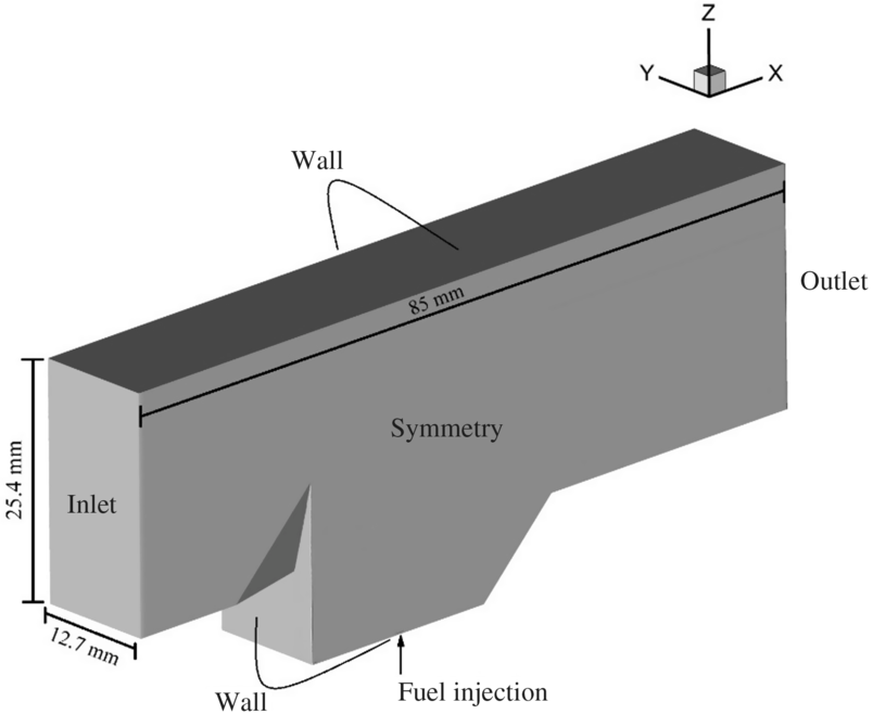
Boundary conditions for the computational domain(Reference Oamjee and Sadanandan28).

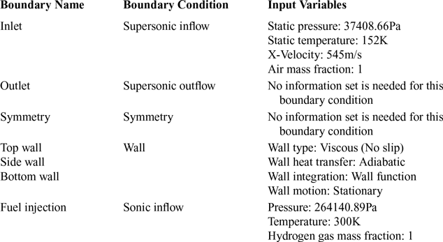
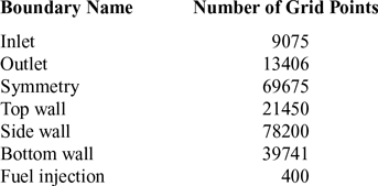
Figure 7 shows the boundary conditions applied for the computational domain. Tables. 2 and 3 give the details regarding the boundary conditions and grid resolution, respectively(Reference Oamjee and Sadanandan28).
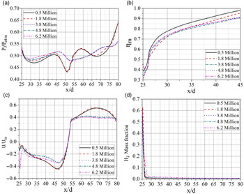
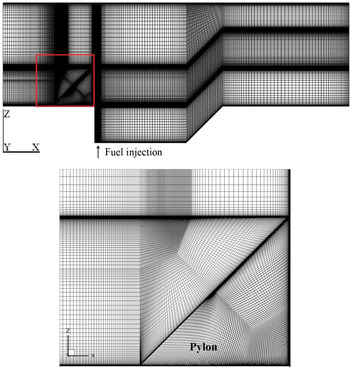
Figure 8 shows the grid independence study on local and global variables over five different meshes with varying grid density and wall spacing. Figure 9 shows the grid generated for the computational domain. It is found that a total of 4.8 million cells with a wall spacing of 0.001mm with a  ${Y^ + }$
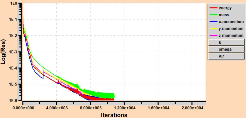
value of 1, can give an acceptable result. The computational domain is initially discretised with 0.5 million cells and refined to finer grid densities until convergence with an error below 1% in local and global variables is observed. CFL number is ramped from 0.1 to 5 for the initial 100 steps. A convergence of the residual that drops by six orders of magnitude can be obtained with less than 20000 iterations (see Fig. 10).
Boundary conditions and input variables

Grid resolution

(a) Local pressure variation along the centre line of the test section (b) mixing efficiency (c) mean X-velocity d) H2 mass fraction variations for various grid refinements for the baseline geometry case(Reference Oamjee and Sadanandan28).

Computational domain grid (top) and the enlarged view of grid in the pylon vicinity shown within the red boundary (bottom)(Reference Oamjee and Sadanandan28).

Residual plot for baseline configuration.

2.2.2 Performance parameters definition
To obtain the data for the performance analysis, the computational domain is divided into 800 sections along the X-axis. Data is extracted along the length of the test section by taking averages over the respective cross sections as defined in(Reference Huang, Li and Yan20). The parameters used for the performance analysis are total pressure loss, mixing efficiency, and flammable plume extent along with fuel jet penetration h/d, where h is the maximum height at which the fuel jet core travels in each cross section and d is the fuel injector diameter.
The present study is considered as a globally fuel-lean system due to a single injection in a large duct configuration. Mixing efficiency is defined as the fraction of the least available reactant that would react if the fuel-air mixture was brought to chemical equilibrium without additional local or global mixing(Reference Fuller, Wu, Nejad and Schetz29). Fuel dispersion magnitude at each cross-section defines the mixing effectiveness  ${\eta _m}$
given by Equation (8).
 \begin{equation}{\eta _m} = \frac{{{{\dot m}_{fuel,mixed}}}}{{{{\dot m}_{fuel,total}}}} = \frac{{\smallint {\alpha _R}\rho UdA}}{{\smallint \alpha \rho UdA}}\end{equation}
 \begin{equation}\alpha = \frac{f}{{f + 1}} = \frac{{\phi {f_s}}}{{\phi {f_s} + 1}}{\rm{\;}}\end{equation}
 \begin{equation}{\alpha _R} = \left\{ {\begin{array}{*{20}{c@{\quad}c}}\alpha , & \alpha \le {\alpha _s}\\[5pt]
\frac{\alpha _s \left( {1 - \alpha } \right)}{1 - \alpha _s}, & \alpha \gt {\alpha _s}\end{array}} \right\}\end{equation}
Mixing effectiveness alone cannot give the complete picture regarding the mixing efficiency rather it provides only the information regarding how well the fuel gets dispersed. To understand mixing efficiency even further, an additional parameter known as fuel plume area fraction  $F{P_f}$
is taken into account. It is defined as the fuel plume area having fuel mass fractions that fall within the flammability limit, normalised by the total fuel plume area for each cross section.
The presence of pylon-cavity and transverse injection results in total pressure loss. It is one of the key parameters which decides the efficiency of a wall-based flameholder configuration when compared to the instream injection models. Equation (11) gives the total pressure loss  $\Lambda$
, which is calculated by the mass averaged integral of total pressure at each cross section.
 ${P_{Tunnel}}$
is the total pressure at the inlet.
 \begin{equation}\Lambda = 1 - \frac{\overline{P_T}}{P_{Tunnel}}\end{equation}
Where,
 \begin{equation}\overline{P}_{T} = \frac{\smallint{P_T}\rho UdA}{\smallint \rho UdA}\end{equation}
3.0 NUMERICAL SCHEME VALIDATION
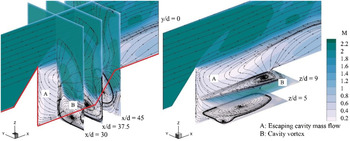
Validation of the computational data has been done with the help of experimentally obtained steady wall pressure data and PIV for the baseline configuration without fuel injection. Figure 11 gives the RANS predicted time averaged streamlines for the baseline configuration. Understanding the flowfield within the pylon-cavity configuration is vital for getting insight into the flow features influencing the fuel mixing process and also the variations observed in the data used for the validation purpose. The presence of pylon ahead of the cavity divides the incoming crossflow to either side of the pylon forming two separate shear layers at the cavity leading edge. These shear layers form a pair of counter-rotating primary vortices (marked B) and smaller corner vortices within the cavity. These vortices help in the cavity mass entrainment process. The low-pressure region at the pylon-cavity wake guides the cavity mass flow that recirculates within the counter-rotating vortices to escape from the cavity (marked A) and take part in the cavity flow-crossflow mass exchange.
Time-averaged streamlines depicted over Mach number contour. The red line represents the outline of the pylon-cavity geometry along the axial plane.

3.1 Steady wall pressure data
Twenty locations on the test section wall are opted for the pressure measurement. A good agreement between the computational and experimental wall pressure data is observed for Mach 2.2 main flow at a total pressure of 4 bar and total temperature of 300K (see Fig. 12). Due to the presence of pylon-cavity geometry, sudden changes in the wall pressure data can be observed at various locations along the axis. A sudden rise in the wall pressure is observed between x/d 10 and 20 downstream of the inlet, which represents the pylon location. Further downstream, immediately after the pylon, a sudden drop in pressure is observed at x/d 20. This is due to the presence of the cavity wake region. There is no significant change in wall pressure data observed at the cavity floor between x/d 20 and 42. Due to the impingement of the shear layer and the mass entrainment process by the crossflow, a rise in wall pressure data is observed at the aftwall (x/d: 45 to 54).
Steady wall pressure data validation for the baseline geometry(Reference Oamjee and Sadanandan28).

3.2 Flow visualization using Schlieren imaging
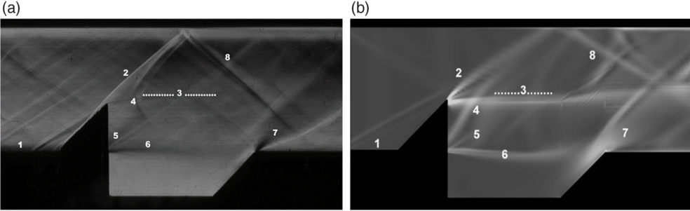
Schlieren imaging helps to visualise various quasi-steady shocks and flow features. Figure 13 shows the comparison of both experimental and numerical Schlieren images for the baseline configuration without any injection. It is evident that there are few differences in the flow features observed when both the images are compared. The experimental Schlieren image show the instantaneous flow features whereas the RANS simulated Schlieren image is time-averaged. The weak shocks seen upstream to the pylon in the experimental Schlieren is a result of the very fine surface irregularities that exist between the different parts of the test section, for example, the 2D nozzle, walls of the test section, pylon geometry, etc. The RANS-simulated Schlieren image shows only a single shock emanating from the leading edge of the computational domain. Also, it is also observed that some of the flow features and shocks shown in numerical Schlieren image are stronger when compared to the instantaneous experimental Schlieren image (e.g. see feature 3 in Fig. 13). This is because the RANS based simulations produce a time averaged value for the flow field quantities. As part of the preliminary validation of the flow field, the RANS based simulations are capable of capturing stronger flow features.
Schlieren image for the baseline configuration (no injection) with various flow features numbered a) experimental b) CFD simulation(Reference Oamjee and Sadanandan28).

Various features visualised are: 1. Incoming boundary-layer; 2. Pylon shock; 3. Pylon wake boundary; 4. Escaping cavity flow interaction with crossflow; 5. Cavity leading edge shock; 6. Cavity shear layer; 7. Ramp shock and expansion; and 8. Pylon shock reflection.
3.3 Particle image velocimetry
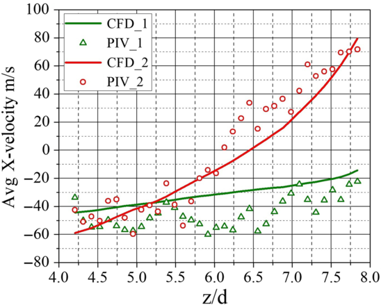
The current study uses 300 image pairs for the velocity vector calculations. Background noise and dark current noise subtraction have been done as part of image pre-processing. The vector field is calculated using the multi-pass option with decreasing interrogation window (IW) size. Initial IW is set to 64 x 64 with an overlap of 50%, wherea, the final IW is set to 16 x 16 with an overlap of 75%. An average correlation value above 0.7 is obtained while processing the image pairs. The minimum detectable shift/shift uncertainty is calculated to be 0.01 pixel or 0.28688m/s. As shown in Fig. 4, the two vertical lines 1 and 2 separated 2mm and 4mm, respectively, from the pylon rear face is used for the validation. Figure 14 shows the comparison of the average X-velocity obtained through PIV and CFD simulations. PIV result shows a good agreement with the CFD simulation values with a maximum deviation of 25m/s.
Comparison of average X-velocity between a) PIV data and b) CFD data along the vertical lines 1 and 2 (see Fig. 4)(Reference Oamjee and Sadanandan28).

4.0 MIXING PERFORMANCE ANALYSIS
For the fuel injection studies, the fundamental geometrical dimensions (L/D, H/D) of the pylon-cavity configuration and experimental conditions are kept the same for all cases. Comparative studies with the baseline geometry (Fig. 3, with fuel injection) using steady state computational simulations are performed to investigate the geometry influence of various pylon-cavity configurations on mixing enhancement.
Figure 15(a) shows that Pylon 1 gives the least total pressure loss. This is due to the reduced effective blockage area of the geometry when compared to other pylon geometries, owing to the three parallel grooves on either side. Since the grooves are parallel to the main flow, the cross-flow momentum is not lost, whereas the other geometries decelerate the cross flow by forming larger recirculation regions behind the pylon. As a result, the capability of Pylon 1 to shield the fuel jet injection from the cavity floor is partially lost. This leads to the loss of fuel jet momentum for the Pylon 1 configuration causing a reduction in fuel jet penetration capability. The reduction in fuel jet penetration for Pylon 2 and Pylon 3 is not significant when compared to the highest penetration height achieved by the baseline geometry (see Fig. 15(b)).
(a) Total pressure loss (b) fuel jet penetration height comparisons.

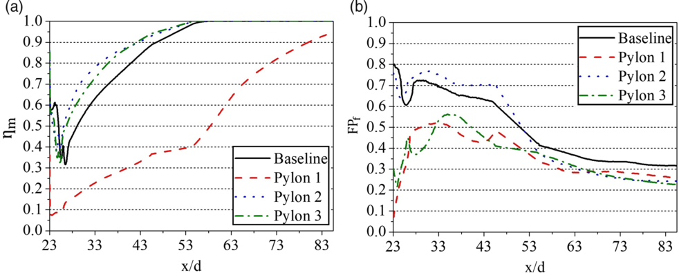
Figure 16(a) shows that Pylon 1 geometry gives the least dispersion of the fuel in the cross flow. This is due to the parallel positioning of the grooves on the pylon surface. The crossflow passes through the grooves without forming any recirculation regions behind the pylon, resulting in an extremely smaller residence time for the air-fuel mixture to get mixed. Whereas the slanted surfaces on Pylon 2, Pylon 3 and baseline pylon improve mixing by forming recirculation regions. Further, when the investigation made among Pylon 2, Pylon 3 and baseline pylon, it is found that the variation in the angle of slants also influences the mixing. Pylon 2 has a combination of inward and outward slanted surfaces, whereas Pylon 3 consist of only outward slanted surface (see Fig. 6). Both the geometries have less effective blockage areas compared to the baseline geometry. As a result, the vortex formation due to Pylon 2 is more when compared to the other two. This gives an enhanced mixing capability for Pylon 2 configuration over other geometries.
(a) Mixing effectiveness (b) flammable plume area fraction comparisons.

To obtain a further understanding of mixing efficiency, the flammable plume area fraction parameter for all the geometries are analysed (see Fig. 16(b)).  $F{P_f}$
gives information about the fraction of the flammable plume area, which is the area consisting of fuel mass fraction that lies within the flammability limit of
 ${{\rm{H}}_2}$
- air mixture (0.14 - 2.54)(Reference Turns30).
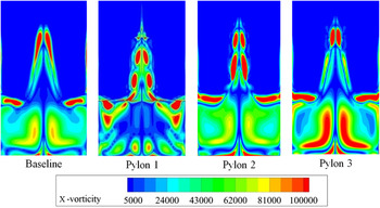
A visual comparison of X-vorticity induced by various pylon geometries is shown in Fig. 17. It is evident that Pylon 2 and Pylon 3 induce more axial vortices across the plane when compared to the baseline and Pylon 1 configurations. This is due to the influence of slanted surfaces present in the geometries and thereby improving the mixing capabilities.
X-vorticity | ${\omega _x}$| induced in the pylon-cavity wake region by different pylon geometries at 6mm downstream from the fuel injection location. The field of view is 25.4mm x 25.4mm.

5.0 CONCLUSION
The primary focus of the current study is to understand the influence of pylon geometry on various performance parameters in a pylon-cavity-aided supersonic combustor of Mach number 2.2. Performance parameters such as mixing efficiency, flammable plume area fraction, fuel jet penetration height and streamwise vorticity measure have been compared for the four different pylon geometries selected for the investigation using steady numerical simulations. The validation of the CFD simulation is performed experimentally with steady wall pressure data, which then used to validate the 2D velocity vector distribution using PIV. Results show that the pylon with reduced effective blockage area to the crossflow with a combination of inward and outward slanted surfaces can give better mixing and flame holding capability with minimal total pressure loss. Cavity and pylon induced vortices have a significant role in creating the recirculation zone within the pylon-cavity region, which can increase the residence time for the air and fuel to get well mixed.
ACKNOWLEDGMENTS
The authors would like to express their thanks to Dr. Aravind Vaidyanathan and Prakash R.S for providing support in conducting the experiments at Advanced Propulsion and Laser Diagnostics (APLD) lab, IIST.