2.1. Upstream heterogeneous mixture

The presence of non-equilibrium perturbations in the upstream gas coming from fuel mass fraction fluctuations must be accompanied with velocity perturbations to consistently satisfy the conservation equations. Similarly, pressure perturbations may be present in the heterogeneous mixture ahead of the shock. When the rotational, acoustic, entropic and composition perturbations result from the same physical mechanism, the corresponding spectra associated with the different types of perturbations are very similar. In particular, for stationary compressible isotropic turbulence (Holzer & Siggia Reference Holzer and Siggia1994; Miller Reference Miller2000), the scalar energy spectra for the fuel mass fraction disturbances peak at the same wave number as the kinetic energy dissipation spectrum, thereby suggesting the use of a similar spectrum form.

The relative influence of the different upstream perturbations on the downstream evolution of the flow depends on the initial perturbation amplitudes and the propagation Mach number. The latter dependence can be investigated using the linearized RH jump conditions, which show that the amplification factor affecting the mass fraction perturbations as they cross the front (with the corresponding changes in density and heat release) remains finite in the limit of large propagation Mach numbers $\mathcal {M}_u \gg 1$, whereas the corresponding amplification factors for the pressure and vorticity perturbations become proportional to $\mathcal {M}_u^{-2}$ and $\mathcal {M}_u^{-1}$, respectively. As result, in the strong-shock limits, the upstream perturbations of vorticity and pressure play a secondary role with regards to the downstream flow.

When dealing multi-component mixtures, the local specific-heat ratio $\gamma$ is also affected by mixture proportions, but this effect can be also neglected in the first approximation. Variations in $\gamma$ are expected to range between $1.1$ and $1.4$ between mixture compounds for light hydrocarbon fuels. Thus, order-of-unity variations in the fuel mass fraction provoke weak changes that are one order of magnitude smaller in the local value of $\gamma$. In addition, even admitting same-order variations in $\gamma$, these perturbations can be neglected for the same reason that velocity and pressure perturbations are not considered, namely they become proportional to $\mathcal {M}_u^{-2}$ in the strong-shock limit.

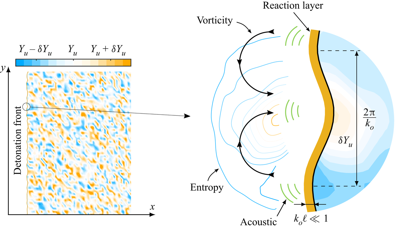
In this work, a planar detonation front is considered to propagate through a heterogeneous gaseous mixture that is static and isobaric, so that the variations of the fuel mass fraction are only associated with perturbations in density and heat release, as sketched in figure 1. It is assumed that the deviation of the local fuel mass fraction $Y_u$ with respect to its average value $\langle Y_u\rangle \sim 1$ is sufficiently small for the linear theory to be applicable, $|\delta Y_u| = |Y_u-\langle Y_u\rangle |\ll 1$. For sufficiently weak perturbations, the isotropic heterogeneous mixture can be approximated by the linear superposition of independent modes, each one being characterized by a wavenumber $\boldsymbol {k}$, so that

(2.1)\begin{equation} \delta Y_u (\boldsymbol{k},\boldsymbol{x}_u)= \varepsilon(\boldsymbol{k})\exp({\textrm{i} \boldsymbol{k} \boldsymbol{\cdot} \boldsymbol{x}_u}), \end{equation}

where $\boldsymbol {x}_u$ is the vector defining the position in a reference frame at rest with respect to the upstream flow, and $\varepsilon (\boldsymbol {k})$ is the amplitude of the fuel mass fraction perturbations corresponding to a given wavenumber vector $\boldsymbol {k}$.

Figure 1.

Sketch of the corrugated detonation front through a heterogeneous gaseous mixture, where the variation of the local fuel mass fraction satisfies $|\delta Y_u|= |Y_u-\langle Y_u\rangle |\ll 1$ in order to apply linear theory. The detonation length $\ell$ is assumed to be much smaller than the characteristic upstream length $k_o^{-1}$.

Assuming that there is no privileged direction in the upstream flow, the spectrum of the fuel mass fraction perturbations is considered spatially homogeneous and isotropic. Thus, the wavenumber vector $\boldsymbol {k}$ is uniformly distributed over the unit sphere (or around the unit semicircle in two dimensions). Therefore, the analysis consists of a superposition of linear perturbations whose amplitudes are exclusively functions of the wavenumber amplitude $k=|\boldsymbol {k}|$. In such cases, the mean square of the fuel mass fraction perturbations in two-dimensional and three-dimensional geometries are

(2.2a,b)\begin{equation} \langle\delta Y_u^2\rangle_\textrm{2D}={\rm \pi} \int_0^{\infty}\varepsilon(k)^2k\,\textrm{d}k \quad \text{and} \quad \langle \delta Y_u^2\rangle_\textrm{3D}=4{\rm \pi} \int_0^{\infty}\varepsilon(k)^2k^2\,\textrm{d}k, \end{equation}

respectively, where $\varepsilon (k)$ represents the spectrum of the fuel mass fraction. When fuel mass fraction perturbations are related to turbulent velocity fluctuations (Holzer & Siggia Reference Holzer and Siggia1994; Miller Reference Miller2000), a plausible but arbitrary choice for the isotropic spectrum may be $\varepsilon (k)^2\sim (k/k_o)^{2}/[1+(k/k_o)^2]^{17/6}$, where $k_o$ is the most representative wavenumber associated to the upstream turbulent flow (Batchelor Reference Batchelor1953; Lee, Lele & Moin Reference Lee, Lele and Moin1993; Sagaut & Cambon Reference Sagaut and Cambon2008; Livescu Reference Livescu2020).

Compared to the detonation front, the fast-reaction model assumes that the detonation thickness is considerably smaller relative to the characteristic wavelength ${\sim } k_o^{-1}$ in the unimodal probability density distributions such that $k_o\ell \ll 1$ as displayed in figure 1. The two length scales are independent of each other. The characteristic scale of the spectrum depends on the type of mixing and turbulence upstream, whereas the detonation thickness mainly depends on the detonation properties through the reaction kinetics and temperature conditions. Although order-of-magnitude differences can be observed between different mixture properties, a rough estimate is 0.01–1 centimetres as a characteristic scale for $\ell$, albeit upstream temperature and detonation overdrive can significantly change this value.

For a generic fuel–air mixture, if the fuel is heavier than air, positive values of $\delta Y_u$ are associated with positive upstream density perturbations, $\delta \rho _u > 0$, and vice versa. The sign of the perturbations of heat release can also be anticipated by taking into account the fact that heat release typically peaks under slightly rich conditions. Thus, positive values of $\delta Y_u$ lead to negative perturbations of heat release, $\delta q_u < 0$, in sufficiently rich environments, while the opposite occurs for lean mixtures.

The small parameter $\delta Y_u$ will be employed below to write the perturbed density and heat release fields as

(2.3)\begin{gather} \rho_u = \langle\rho_u\rangle+\delta \rho_u = \langle\rho_u\rangle(1+\delta Y_u W), \end{gather}

(2.4)\begin{gather}q_u = \langle q_u\rangle + \delta q_u = \langle q_u\rangle(1+\delta Y_u H), \end{gather}

where the parameters $W = \rho _u^{-1}(\textrm {d}\rho _u/\textrm {d}Y_u)$ and $H = q_u^{-1} (\textrm {d} q_u/\textrm {d} Y_u)$ relate to the local slopes of the $\rho _u (Y_u)$ and $q_u(Y_u)$ curves, respectively. For a ‘binary’ fuel–air mixture with fuel and air mass fractions being $Y_u$ and $1-Y_u$, the dependence of the mixture density and the dimensionless function $W$ with the fuel mass fraction is noted as

(2.5a,b)\begin{equation} \frac{\rho_u}{\rho_a} = \frac{1}{1-\left(1-\dfrac{W_A}{W_F}\right)Y_u} \quad \text{and} \quad W = \frac{1}{\rho_u}\frac{\textrm{d} \rho_u}{\textrm{d} Y_u} =\frac{1-\dfrac{W_A}{W_F}}{1-\left(1-\dfrac{W_A}{W_F}\right)Y_u}, \end{equation}

where $\rho _a$ is the air density, and $W_A$ and $W_F$ refer to the air and fuel molecular weights, respectively.

The variation of the heat release with the fuel mass fraction cannot be accurately anticipated because it depends on the final composition of the burnt mixture. Detonations induce a strong compression work – through the irreversible transformation made by the shock – and a later expansion of the fluid, which makes the final temperature differ from the adiabatic flame temperature of isobaric combustion. It is widely known however that heat release peaks close to stoichiometric conditions for slightly rich mixtures, a property that can be used to anticipate the sign of the slope of the heat release-fuel mass fraction curve. Accurate values of $q_u$ can be obtained with either numerical codes or experimental data.

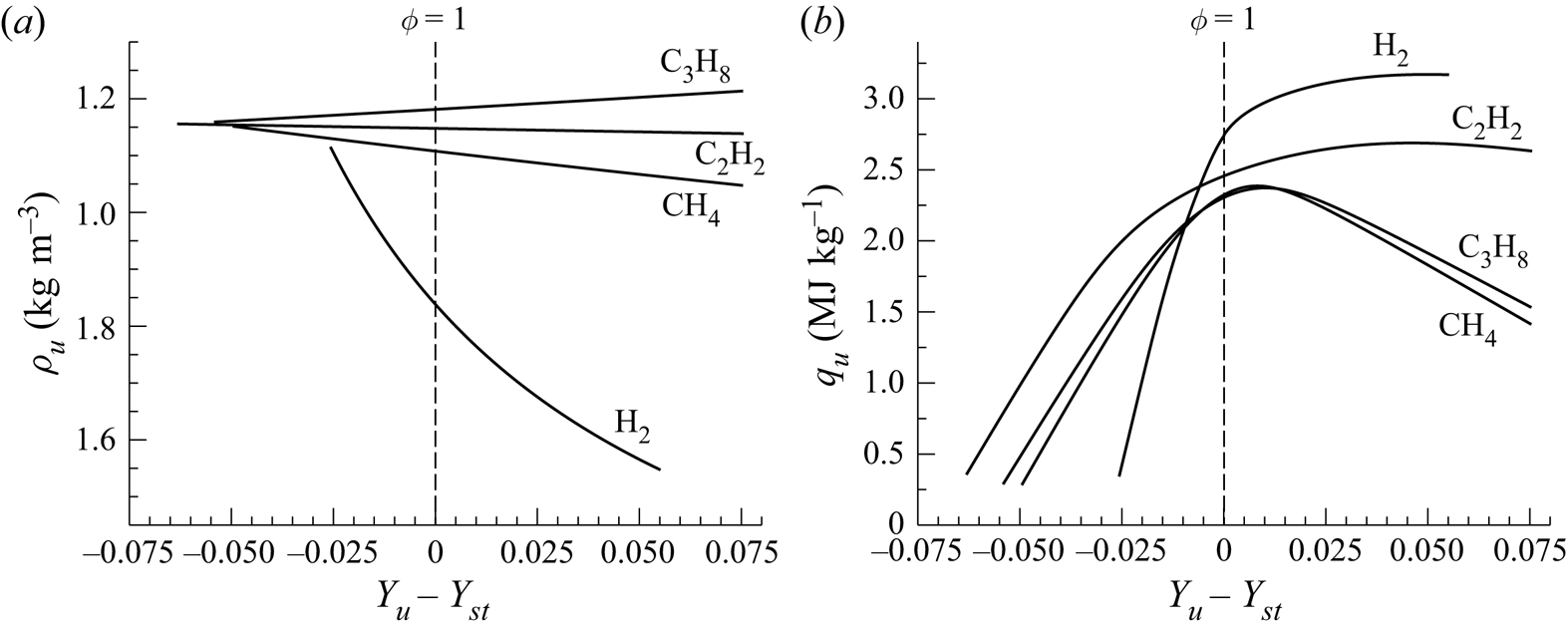
Figure 2 has been computed with an in-house thermochemical code validated with NASA-CEA (Gordon & McBride Reference Gordon and McBride1994) and CANTERA (Goodwin et al. Reference Goodwin, Speth, Moffat and Weber2018), including Caltech's shock and detonation toolbox (Browne, Ziegler & Shepherd Reference Browne, Ziegler and Shepherd2008). Here, the variation of density (a) and heat release (b) with the fuel mass fraction is shown for different gases, including hydrogen (H$_2$), methane (CH$_4$), acetylene (C$_2$H$_2$) and propane (C$_3$H$_8$), with stoichiometric fuel mass fractions $Y_{st}= 0.0285$, $0.0552$, $0.0705$ and $0.0603$, respectively. 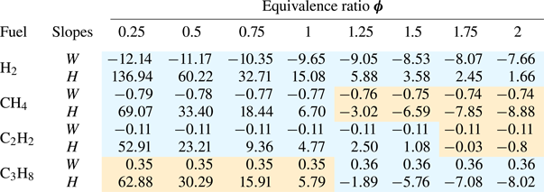Representative values of $W$ and $H$ obtained from these computations are given in table 1 for these fuels and different equivalence ratios ranging from very lean to moderately rich mixtures.

Figure 2.

Variation of density (a) and heat release (b) with the fuel mass fraction for representative fuel–air mixtures. The dashed line represents the stoichiometric condition given by $Y_{u}=Y_{st}$$(\phi = 1)$. Computations are given for hydrogen, methane, acetylene and propane at $300$ K and $10^5$ Pa in fresh conditions. The associated stoichiometric fuel mass fractions are $Y_{st}=0.0285$, $0.0552$, $0.0705$ and $0.0603$, respectively.

Table 1.

Dimensionless slopes of the density and heat release curves, $W$ and $H$, for H$_2$, CH$_4$, C$_2$H$_2$ and C$_3$H$_8$. The orange and blue background colours are applied for positive and negative values of the relation $H/W$, respectively.

2.2. Homogeneous Rankine–Hugoniot equations

Neglecting the deviation from the mean values, the flow variables in the burnt gas are obtained by integrating the conservation equations in the streamwise direction, yielding

(2.6a)\begin{gather} \rho_u u_u = \rho_d u_d, \end{gather}

(2.6b)\begin{gather}p_u + \rho_u u_u^2 = p_d + \rho_d u_d^2, \end{gather}

(2.6c)\begin{gather}h_u + \tfrac{1}{2} u_u^2 = h_d + \tfrac{1}{2} u_d^2, \end{gather}

for the mass, streamwise momentum and energy conservation equations, respectively. Here, the subscripts $u$ and $d$ refer to the upstream and downstream dimensional flow properties, respectively, including the velocity $u$, density $\rho$ (or specific volume $V = \rho ^{-1}$), pressure $p$ and enthalpy $h$. The upstream flow comprises a mixture of gases, each of which is modelled as a calorically perfect gas, i.e. the specific heats, and, therefore, the adiabatic index $\gamma$ are assumed to be constant throughout the shock compression and combustion processes. Thus, the enthalpy variation is written as a function of a single value of $\gamma$,

(2.7)\begin{equation} h_d-h_u = q_u + \frac{\gamma}{\gamma -1}\left(\frac{p_d}{\rho_d}-\frac{p_u}{\rho_u} \right), \end{equation}

where $q_u$ represents the heat released in the reaction front per unit mass of mixture. In realistic conditions, the value of $\gamma$ depends on both mixture composition and temperature, which experience significant changes across the detonation wave. In qualitative terms, when the effect of temperature dominates the variation of $\gamma$ by the excitation of vibrational modes, the specific heat ratio is expected to monotonically decrease with temperature. However, given that a change in the structure of the molecules exists as a result of the combustion process, the total variation of $\gamma$ must include information of the initial and final composition of the mixture. However, since upstream thermal energy can be neglected in the first approximation, the value used in the computations should be the value associated with the burnt-gas conditions to minimize the error when $\gamma$ is constant.

Algebraic manipulation of (2.6a)–(2.7) provides the jump equations across the reaction front, namely,

(2.8)\begin{align} \mathcal{R}_d = \frac{\rho_d}{\rho_u} &= \frac{( \gamma + 1) {\mathcal{M}}_u^2}{\gamma {\mathcal{M}}_u^2 +1- [({\mathcal{M}}_u^{2}-1)^2 -4 Q {\mathcal{M}}_u^{2} ]^{1/2}}, \end{align}

(2.9)\begin{align} \mathcal{P}_d = \frac{p_d}{p_u} &= \frac{\gamma {\mathcal{M}}_u^2 +1+ \gamma [({\mathcal{M}}_u^{2}-1)^2 -4 Q {\mathcal{M}}_u^{2} ]^{1/2}}{\gamma + 1} \nonumber\\ &= \frac{(\gamma +1){\mathcal{R}}_d-\gamma+1 +4 {\mathcal{R}}_d Q \gamma/(\gamma+1)}{\gamma +1-(\gamma-1){\mathcal{R}}_d } \end{align}

for density and pressure, respectively, while the Mach number of the burnt-gas flow is

(2.10)\begin{equation} {\mathcal{M}}_d = \frac{u_d}{a_d} = \left\{\frac{\gamma {\mathcal{M}}_u^2 +1- [({\mathcal{M}}_u^{2}-1)^2 -4 Q {\mathcal{M}}_u^{2} ]^{1/2}}{\gamma {\mathcal{M}}_u^2 +1+ \gamma [({\mathcal{M}}_u^{2}-1)^2 -4 Q {\mathcal{M}}_u^{2} ]^{1/2}}\right\}^{1/2}, \end{equation}

where $a_d$ denotes the speed of sound and

(2.11)\begin{equation} Q = \frac{(\gamma^2-1)}{2 a_u^2}q_u \end{equation}

is the dimensionless heat release per unit mass.

The so-called Chapman–Jouguet (CJ) condition, which is given by $({\mathcal {M}}_u^{2}-1)^2 -4 Q {\mathcal {M}}_u^{2}=0$, defines the minimum detonation strength. Thus, the maximum downstream Mach number is associated with a given energy release as follows:

(2.12)\begin{equation} \mathcal{M}_{cj}=\left(1+Q\right)^{1/2}+Q^{1/2}. \end{equation}

This value is related to the maximum flow expansion of the hot gases in the reaction layer. Within this subsonic region behind the shock, the flow is expanded up to sonic conditions, ${\mathcal {M}}_d=1$, corresponding to the well-known Chapman–Jouguet condition for detonation waves. As a result, the detonation wave decouples from downstream influences, and its motion is self-sustained by the expansion of the products resulting from the exothermic transformation.

2.3. Linear interaction analysis

As illustrated in figure 2 and table 1, deviations in the fuel mass fraction are often accompanied by perturbations in density and/or heat release. Depending on the particular conditions, i.e. type of fuel and average equivalence ratio of the unburnt mixture, the dimensionless slope $H$ may reach values of order 10 or greater. It also occurs with the function $W$ in hydrogen–air mixtures (or any other fuel much heavier than air not shown in the table). This finding suggests that $\delta Y_u$ may not be a good reference scale for the upstream perturbation field given that linear (small) variations in the fuel mass fraction may be associated with nonlinear (large) perturbations in $\rho _u$ and/or $q_u$. For any flow condition, to ensure that small changes $\delta Y_u$ do not lead to large input perturbations into the system, the small parameter should simply be redefined in the form $\epsilon (k) = \varepsilon (k)\sqrt {W^2+H^2}$, and $\epsilon (k) \ll 1$ is a requirement. Thus, even if $W$ or $H$ are large compared to unity, the perturbations in the fuel mass fraction will be sufficiently small for all flow perturbations to remain within the limits of linear theory. Similarly, larger fuel mass fraction perturbations will be permitted for $W \sim H\ll 1$.

When written in a reference frame moving with the detonation front, $x_l = u_u t$, the upstream density and heat release perturbations can be written as

(2.13)\begin{equation} \hat{\rho}_u=\frac{\delta \rho_u}{\langle\rho_u\rangle } = \epsilon(k) \frac{W}{\sqrt{W^2+H^2}}\exp [{\textrm{i}(k_x u_u t + k_y y + k_z z)}] \end{equation}

and

(2.14)\begin{equation} \hat{q}_u=\frac{\delta q_u}{\langle q_u\rangle } = \epsilon(k) \frac{H}{\sqrt{W^2+H^2}} \exp [{\textrm{i}( k_x u_u t + k_y y + k_z z)}], \end{equation}

where use is composed of (2.1), (2.3) and (2.4) and the above definition of $\epsilon (k)$. The pre-exponential factors $W/\sqrt {W^2+H^2}$ and 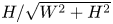$H/\sqrt {W^2+H^2}$ represent the relative effects on density and heat release fluctuations of a small change of the fuel mass fraction. A closer inspection of the RH jump relationships shows that positive values of $\delta \rho _u$ and $\delta q_u$ result in higher downstream pressures. In terms of fuel mass fraction perturbation $\delta Y_u$, constructive effects are to be expected in lean heavy-fuel or rich light-fuel mixtures, while destructive contributions will occur in lean light-fuel or rich heavy-fuel mixtures.

Using the modulus of the wavenumber vector $k$ and its product with the speed of sound in the burnt gas $a_d k$ as characteristic spatial and temporal frequencies, the spatio-temporal variables can be written in non-dimensional form as $(\hat {x},\hat {y},\hat {z})= k\boldsymbol {x}$ and $\tau = a_d k t$, where $\boldsymbol {x}$ is measured in the burnt-gas reference frame. However, it is always possible to simplify the formulation by rotating the reference frame around the direction of propagation of the detonation such that only two spatial coordinates remain in the problem: one in the axis of the detonation propagation, $\hat {x}$, and the other perpendicular to it at any arbitrary direction, $\hat {y}$.

The linear perturbations in the burnt gas are defined with functions of order unity (denoted with a hat symbol) and scaled with the small parameter $\epsilon$, namely

(2.15a)\begin{gather} p(x,y,\tau) = \rho_d a_d^2 [\gamma^{-1}+\epsilon\ \hat{p}(\hat{x},\hat{y},\tau)], \end{gather}

(2.15b)\begin{gather}\rho(x,y,\tau) = \rho_d [1+\epsilon\ \hat{\rho}(\hat{x},\hat{y},\tau)], \end{gather}

(2.15c)\begin{gather}u(x,y,\tau) = a_d [{\mathcal{M}}_d({\mathcal{R}}_d-1)+\epsilon\ \hat{u}(\hat{x},\hat{y},\tau)], \end{gather}

(2.15d)\begin{gather}v(x,y,\tau) = a_d \epsilon\ \hat{v}(\hat{x},\hat{y},\tau), \end{gather}

which are introduced in the Euler equations to give

(2.16a)\begin{gather} \frac{\partial \hat{\rho}}{\partial \tau}=-\frac{\partial \hat{u}}{\partial \hat{x}}-\frac{\partial \hat{v}}{\partial \hat{y}}, \end{gather}

(2.16b)\begin{gather}\frac{\partial \hat{u}}{\partial \tau}=-\frac{\partial \hat{p}}{\partial \hat{x}}, \end{gather}

(2.16c)\begin{gather}\frac{\partial \hat{v}}{\partial \tau}=-\frac{\partial \hat{p}}{\partial \hat{y}}, \end{gather}

(2.16d)\begin{gather}\frac{\partial \hat{\rho}}{\partial \tau}=\frac{\partial \hat{p}}{\partial \tau}. \end{gather}

The system of linear equations must be supplemented by the boundary conditions associated to isolated detonation. As the burnt-gas flow field reduces to linear gas dynamics within the domain contained between $\hat {x}=-\tau + c_t$ (first left-travelling acoustic wave) and $\hat {x}={\mathcal {M}}_d\tau + c_t$ (detonation front position) in the $\hat {x} - \tau$ plane. The arbitrary constant $c_t$, which is defined with the temporal reference frame, does not play any role in the long-time asymptotic analysis.

For the sake of simplicity, the isolated assumption is considered in this work, which translates into the omission of front-travelling waves reaching the detonation wave from behind. As a direct consequence, the detonation is only excited with the monochromatic perturbation of the upstream flow, thereby resulting in a single oscillation frequency $\omega _d = (k_x/k)(u_u/a_d) = \kappa _x \mathcal {R}_d\mathcal {M}_d$, where $\kappa _i=k_i/k$ for $i= \{x,y,z\}$ is the dimensionless wave number component of the upstream flow. Linearized RH relationships, which involve the perturbation of the detonation position with respect to its planar form $\xi _d= k [x_{l,s}(t)-u_u t]$,

(2.17a)\begin{gather} \frac{{\mathcal{R}}_d-1}{{\mathcal{R}}_d} \frac{\textrm{d}\xi_d}{\textrm{d}\tau} = \frac{1-\varGamma}{2 {\mathcal{M}}_d}\hat{p}_d -\frac{{\mathcal{M}}_d\left({\mathcal{R}}_d-2+\varDelta \right)W-{\mathcal{M}}_d \left(1-\varDelta\right)H}{2\sqrt{W^2+H^2}}\textrm{e}^{-\textrm{i}\omega_d \tau}\,\textrm{e}^{\textrm{i}\kappa_y \hat{y}}, \end{gather}

(2.17b)\begin{gather}\hat{u}_d = \frac{1+\varGamma}{2 {\mathcal{M}}_d}\hat{p}_d-\frac{{\mathcal{M}}_d\left({\mathcal{R}}_d-\varDelta \right)W+{\mathcal{M}}_d \left(1-\varDelta\right)H}{2\sqrt{W^2+H^2}}\textrm{e}^{-\textrm{i}\omega_d \tau}\,\textrm{e}^{\textrm{i}\kappa_y \hat{y}}, \end{gather}

(2.17c)\begin{gather}\hat{\rho}_d = \frac{\varGamma}{{\mathcal{M}}_d^2}\hat{p}_d+ \frac{{\rm \Delta} W - \left(1-\varDelta\right)H}{\sqrt{W^2+H^2}}\textrm{e}^{-\textrm{i}\omega_d \tau}\,\textrm{e}^{\textrm{i}\kappa_y \hat{y}}, \end{gather}

(2.17d)\begin{gather}\hat{v}_d = - {\mathcal{M}}_d\left({\mathcal{R}}_d-1\right)\frac{\partial\xi_d}{\partial \hat{y}}, \end{gather}

are employed to calculate the amplitudes accompanying the factor $\textrm {e}^{-\textrm {i}\omega _d \tau }\,\textrm {e}^{\textrm {i}\kappa _y \hat {y}}$ in the non-dimensional perturbations. The quantity

(2.18)\begin{equation} \varGamma = \frac{p_d-p_u}{V_u-V_d}\left.\frac{\textrm{d} V}{\textrm{d} p}\right|_{d}= \frac{\gamma {\mathcal{M}}_u^2}{ {\mathcal{R}}_d^2}\left(\frac{ \partial {\mathcal{P}}_d}{ \partial {\mathcal{R}}_d}\right)^{-1} \end{equation}

measures the slope of the RH curve relative to the Rayleigh–Mickelson line, and the term

(2.19)\begin{equation} \varDelta=\frac{1 + Q {\mathcal{R}}_d \left(\dfrac{\gamma-1}{\gamma+1}\right)}{1+Q} < 1 \end{equation}

accounts for the variation of the post-detonation state due to the upstream changes in density and heat release.

Note that the linear perturbation variables admit the breakdown in terms of potential (acoustic) and entropic–rotational contributions (Kovasznay Reference Kovasznay1953; Chu & Kovásznay Reference Chu and Kovásznay1958). The former takes the form of travelling waves, while the latter remains steady in the reference frame moving with the burnt-gas particles in the absence of diffusive effects. This property is exploited in the normal mode analysis performed in appendix A, where the transfer functions describing the amplitude of the burnt-gas perturbation modes as a function of the detonation properties is described.

3.1. Turbulent kinetic energy

An important feature that deserves particular attention is the turbulence kinetic energy generated by the wrinkled detonation front. When scaled with the square of the sound speed in the burnt gas, it can be expressed as

(3.1)\begin{equation} \textrm{TKE}_\textrm{2D}=\frac{1}{2}\frac{\langle \delta v_i \delta v_i\rangle}{a_d^2}= \frac{1}{2}\langle\hat{u}^2+\hat{v}^2\rangle_\textrm{2D} \int_0^\infty\epsilon (k)^2 k\,\textrm{d} k = \frac{1}{2} \langle\hat{u}^2+\hat{v}^2\rangle_\textrm{2D}\langle \delta Y_u^2 \rangle_\textrm{2D}, \end{equation}

with

(3.2)\begin{equation} \langle\hat{u}^2+\hat{v}^2\rangle_\textrm{2D} =\frac{2}{\rm \pi}\int_0^{{\rm \pi}/2}\left(|\hat{u}|^2+|\hat{v}|^2\right) \textrm{d} \theta, \end{equation}

provided $\langle \delta Y_u^2\rangle _\textrm {2D}$ is known from (2.2a,b). Thanks to the isotropy condition of the perturbation field, the influence of the shape of the spectrum enters as an integral contribution that can be factored out. Equivalent three-dimensional computations can be performed by defining

(3.3)\begin{equation} \langle\hat{u}^2+\hat{v}^2\rangle_\textrm{3D} =\int_0^{{\rm \pi}/2}\left(|\hat{u}|^2+|\hat{v}|^2\right) \sin\theta\,\textrm{d} \theta, \end{equation}

where $\hat {u}$ and $\hat {v}$ are the streamwise and transverse velocity components. The normalization criterion applied is that $\langle \hat {u}^2+\hat {v}^2\rangle _{\textrm {2D}, \textrm {3D}}$ must be equal to unity when the integrand function is spatially uniform and equal to unity.

In the far-field asymptotic regime, the kinetic energy can be conveniently computed by accounting for the separate contributions of the rotational and acoustic velocity fields $\langle \hat {u}^2+\hat {v}^2\rangle =\langle \hat {u}_r^2+ \hat {v}_r^2 \rangle +\langle \hat {u}_a^2 +\hat {v}_a^2\rangle$, to give

(3.4)\begin{equation} \left.\begin{gathered} \langle\hat{u}^2+\hat{v}^2\rangle_\textrm{2D} = \frac{2}{\rm \pi}\int_0^{{\rm \pi}/2} (\mathbb{U}_r^2+\mathbb{V}_r^2) \textrm{d} \theta+\frac{2}{\rm \pi} \int_0^{\theta_c}(\mathbb{U}_a^2+\mathbb{V}_a^2) \textrm{d} \theta, \\ \langle\hat{u}^2+\hat{v}^2\rangle_\textrm{3D} =\int_0^{{\rm \pi}/2}(\mathbb{U}_r^2+\mathbb{V}_r^2) \sin\theta\,\textrm{d}\theta+\int_0^{\theta_c}(\mathbb{U}_a^2+\mathbb{V}_a^2) \sin\theta\,\textrm{d} \theta, \end{gathered}\right\} \end{equation}

where the amplitudes $\mathbb {U}_r$, $\mathbb {V}_r$, $\mathbb {U}_a$, and $\mathbb {V}_a$, provided in appendix A, are explicit functions of $\theta =\tan ^{-1}(k_y/k_x)$ and the remaining governing parameters: $\gamma$, ${\mathcal {M}}_u$, $Q$, $W$, and $H$. To compute the rotational contribution one must separate the high-frequency and low-frequency amplitudes, as given in (A29), which must be integrated over the two different domains $\int _0^{\theta _c}(\ldots )\,\textrm {d}\theta$ and $\int _{\theta _c}^{{\rm \pi} /2}(\dots )\,\textrm {d}\theta$, respectively.

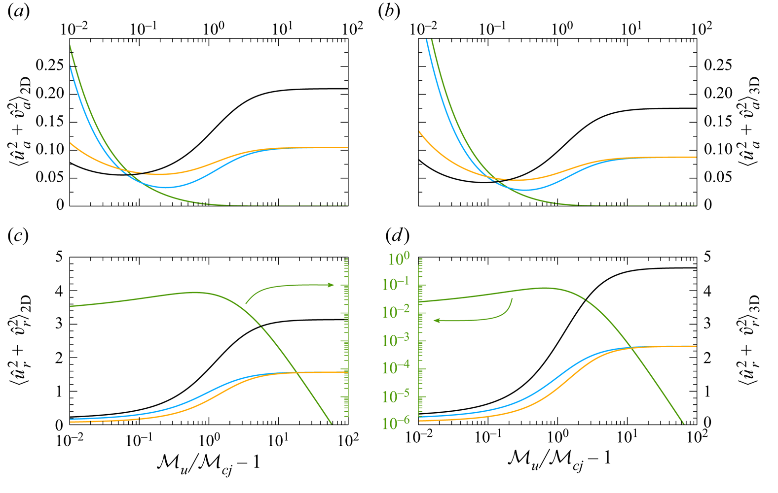
Figure 3 shows the acoustic (a,b) and rotational (c,d) contributions to the total kinetic energy in both two-dimensional (a and c) and three-dimensional (b and d) isotropic configurations. The averages are plotted as a function of the overdrive parameter 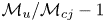$\mathcal {M}_u/\mathcal {M}_{cj}-1$. The correlation between $W$ and $H$ has a strong impact on the generation of turbulent kinetic energy. 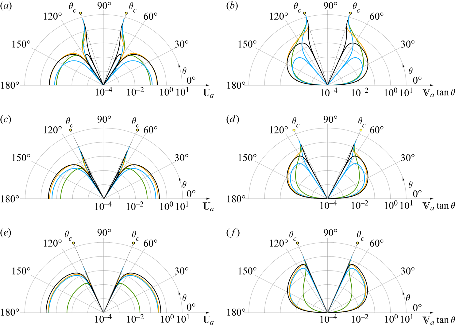For example, heat release variations, either for $|H|\gg |W|$ or $H=-W$, produce higher levels of acoustic energy when the overdrive is small, a finding that can be anticipated with the normal mode analysis, as shown in figure 14 in appendix A. The unbounded growth of the acoustic perturbations in the CJ condition warns about the limits of validity of the linear thin-detonation model, which gains in reliability as the overdrive increases.

Figure 3.

Acoustic (a,b) and rotational (c,d) contributions to the turbulent kinetic energy in 2D (a and c) and 3D (b and d) geometries. Computations are shown as a function of the overdrive parameter $\mathcal {M}_u/\mathcal {M}_{cj}-1$ for $\gamma =1.2$, $Q = 1$, and $|W|\gg |H|$ (black lines), $|H|\gg |W|$ (green lines), $W=H$ (orange lines) and $W=-H$ (blue lines).

The cases selected for the calculations and the associated colour code will be maintained in the following figures. In all the plots, the black curves correspond to the reference case where the upstream perturbation field is dominated by density changes, as in Huete et al. (Reference Huete, Sánchez and Williams2013). In this case, the average fuel mass fraction is close to the peak of heat release, which leads to a negligible contribution of heat release variations with the fuel mass fraction. As an opposite limit, the green curves represent cases where heat release variations dominate over density changes, which is applicable to mixtures of gases with similar density and located far-off the heat release peak. The other two distinguished cases refer to positive (orange) and negative (blue) correlations of density and heat release perturbations. The former is applicable to light fuel–air mixtures ($W_F < W_A$) in sufficiently rich conditions or heavy mixtures ($W_F > W_A$) in sufficiently lean conditions. On the other hand, negative correlations are applicable to light fuel–air mixtures in sufficiently lean conditions or heavy fuel–air mixtures in sufficiently rich conditions. Four examples are given in table 1 where the orange and blue background colours denote the mentioned positive and negative correlations, respectively.

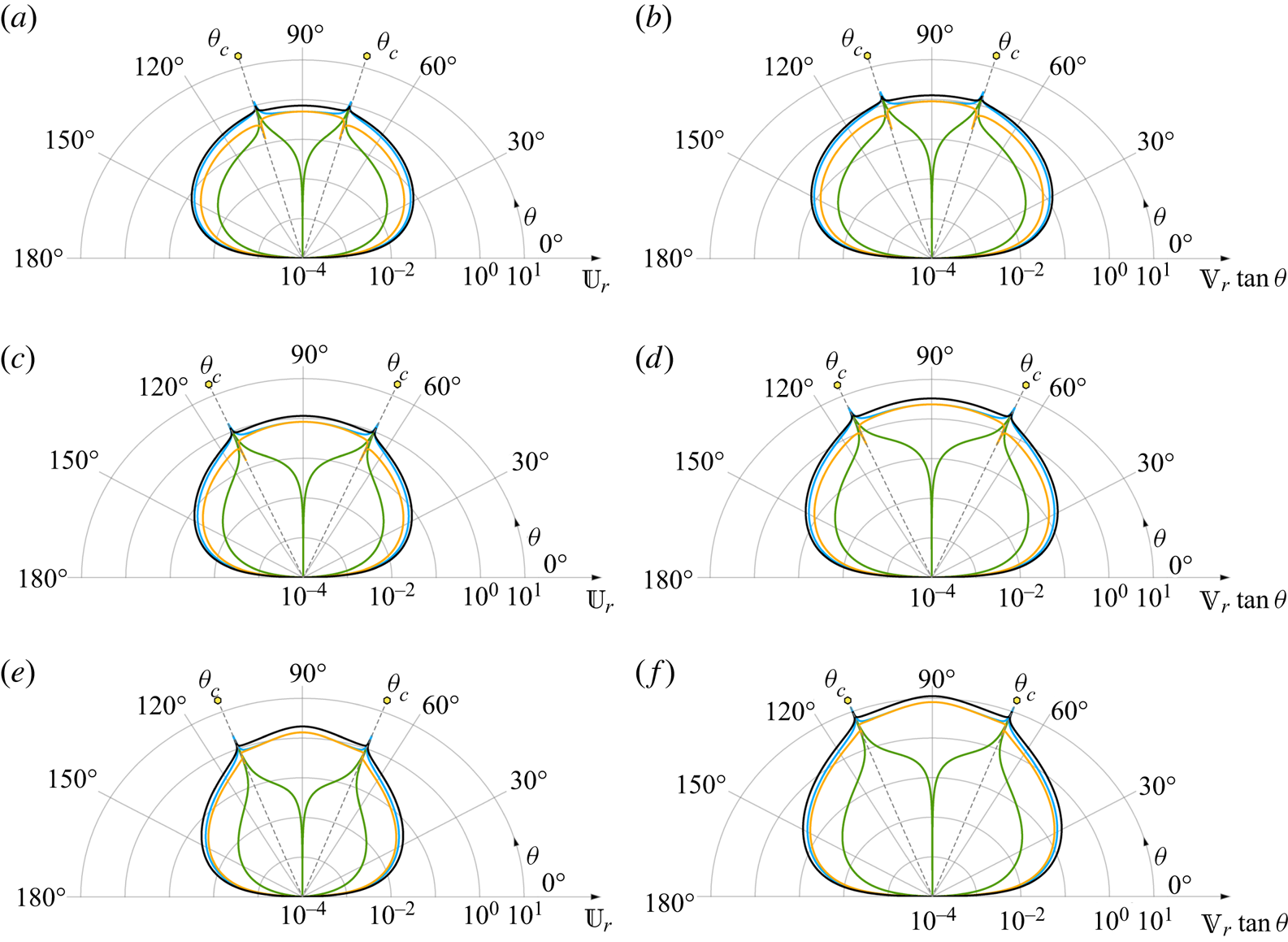
Regarding the rotational contribution, the degree of overdrive does not modify the hierarchy of effects associated to the correlation between $H$ and $W$ for one single frequency, as displayed in figure 15 in appendix A. Note that the case $|H|\gg |W|$ (green lines) uses its own log–log scale, which is shown between subplots (c) and (d), because it would have been impossible to distinguish it from the horizontal axis otherwise. With this consideration in mind, it is seen that the case with exclusively density perturbations yields the highest intensity of turbulence generation, and the effect of heat release is to cushion the kinetic energy deposited in the form of eddies behind the detonation wave. The results also show that the rotational contribution dominates the generation of turbulent kinetic energy over the acoustic field by one order of magnitude, except for weakly overdriven detonations, when both become the same order. Some features in figure 3 are similar for the acoustic and rotational contributions. For example, the qualitative picture of two-dimensional and three-dimensional cases is very similar. In addition, density disturbances dominate for finite to high degrees of overdrives. Thus, the turbulent kinetic energy generated for $|H|\gg |W|$ is much smaller and tends to zero with the overdrive, while the cases $H=-W$ and $H=W$ render similar values for strongly overdriven detonations, an asymptotic value that corresponds to the half of that obtained for $|W|\gg |H|$. The latter is easily deduced from (2.13) since the relative amplitude of the density field squared, $W^2/(W^2+H^2)$, is unity for $|W|\gg |H|$ and 1/2 for $H=\pm W$, while the relative amplitude of the heat release field squared, $H^2/(W^2+H^2)$, vanishes for $|W|\gg |H|$.

The breakdown of longitudinal and transverse contributions of the kinetic energy can be computed separately as

(3.5)\begin{equation} \left.\begin{gathered} \langle\hat{u}^2\rangle_\textrm{2D} =\langle \hat{u}_r^2 \rangle_\textrm{2D} + \langle \hat{u}_a^2 \rangle_\textrm{2D}= \frac{2}{\rm \pi}\int_0^{{\rm \pi}/2} \mathbb{U}_r^2\,\textrm{d} \theta +\frac{2}{\rm \pi}\int_0^{\theta_c}\mathbb{U}_a^2\, \textrm{d} \theta, \\ \langle\hat{u}^2\rangle_\textrm{3D} =\langle \hat{u}_r^2 \rangle_\textrm{3D} + \langle \hat{u}_a^2 \rangle_\textrm{3D}= \int_0^{{\rm \pi}/2}\mathbb{U}_r^2 \sin\theta\, \textrm{d} \theta +\int_0^{\theta_c}\mathbb{U}_a^2 \sin\theta\,\textrm{d} \theta, \end{gathered}\right\} \end{equation}

and

(3.6)\begin{equation} \left.\begin{gathered} \langle\hat{v}^2\rangle_\textrm{2D} =\langle \hat{v}_r^2 \rangle_\textrm{2D} + \langle \hat{v}_a^2 \rangle_\textrm{2D}= \frac{2}{\rm \pi}\int_0^{{\rm \pi}/2}\mathbb{V}_r^2\,\textrm{d} \theta +\frac{2}{\rm \pi}\int_0^{\theta_c}\mathbb{V}_a^2\ \textrm{d} \theta, \\ \langle\hat{v}^2\rangle_\textrm{3D} =\langle \hat{v}_r^2 \rangle_\textrm{3D} +\langle \hat{v}_a^2 \rangle_\textrm{3D}=\int_0^{{\rm \pi}/2} \mathbb{V}_r^2 \sin\theta\,\textrm{d} \theta + \int_0^{\theta_c}\mathbb{V}_a^2 \sin\theta\,\textrm{d} \theta,\end{gathered}\right\} \end{equation}

respectively, where $\langle \hat {u}^2+\hat {v}^2\rangle _\textrm {2D,3D}^{\,}=\langle \hat {u}^2\rangle _\textrm {2D,3D}^{\,}+\langle \hat {v}^2\rangle _\textrm {2D,3D}^{\,}$ for both rotational and acoustic contributions, independently.

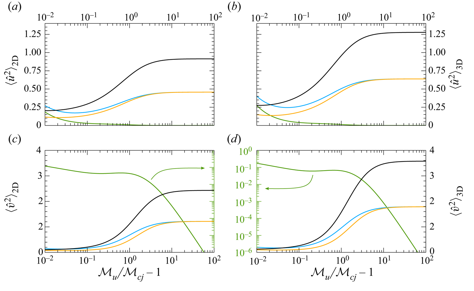
Figure 4 shows the average streamwise (a,b) and transverse (c,d) contributions to the total kinetic energy in both two-dimensional (a and c) and three-dimensional (b and d) isotropic flows. The averages are plotted as a function of the overdrive parameter 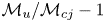$\mathcal {M}_u/\mathcal {M}_{cj}-1$. In consonance with figure 15, the lateral component is higher than the longitudinal part. As expected, the strong-shock limit is governed by the density-induced turbulence in both longitudinal and transverse contributions. In the case $|H|\gg |W|$, shown on its own log–log scale, the turbulence generation is very weak over most of the overdrive domain. For weakly overdriven detonations, however, the effect of heat release variations has a non-negligible impact in the generation of turbulence, which, as observed in figure 3, is mainly derived from the acoustic contribution. In agreement with the previous plot, for three-dimensional random isotropic fields, the generation of turbulence is more intense for both lateral and streamwise components, and negative correlations render higher levels of turbulence. Thus, when the fuel mass fraction is outside the heat release peak, turbulence generation is expected to be enhanced from the hydrodynamical point of view in light fuel–air mixtures in sufficiently lean conditions or heavy fuel–air mixtures in sufficiently rich conditions.

Figure 4.

Longitudinal (a,b) and transverse (c,d) contributions to the turbulent kinetic energy in 2D (a and c) and 3D (b and d) geometries. Computations are shown as a function of the overdrive parameter $\mathcal {M}_u/\mathcal {M}_{cj}-1$ for $\gamma =1.2$, $Q = 1$, and $|W|\gg |H|$ (black lines), $|H|\gg |W|$ (green lines), $W=H$ (orange lines) and $W=-H$ (blue lines).

3.2. Enstrophy and averaged pressure and density fields

The average rotational motion behind the detonation can be measured by the so-called enstrophy that takes the form

(3.7a,b)\begin{equation} \langle\varOmega^2 \kappa_y^2\rangle_\textrm{2D} =\frac{2}{\rm \pi}\int_0^{{\rm \pi}/2}\mathbb{O}^2 \sin^2\theta \,\textrm{d} \theta,\quad \langle\varOmega^2 \kappa_y^2\rangle_\textrm{3D} =\int_0^{{\rm \pi}/2}\mathbb{O}^2\sin^3\theta\, \textrm{d} \theta, \end{equation}

where $\mathbb {O}$ must be evaluated from (A 25) in appendix A and $\kappa _y = \sin \theta$. By similar arguments, the averaged values of the squared density perturbations are

(3.8)\begin{equation} \left.\begin{gathered} \langle\hat{\rho}^2\rangle_\textrm{2D} =\langle \hat{\rho}_e^2 \rangle_\textrm{2D} + \langle \hat{\rho}_a^2 \rangle_\textrm{2D}= \frac{2}{\rm \pi}\int_0^{{\rm \pi}/2}\mathbb{D}_e^2\,\textrm{d} \theta + \frac{2}{\rm \pi}\int_0^{\theta_c}\mathbb{D}_a^2\,\textrm{d} \theta, \\ \langle\hat{\rho}^2\rangle_\textrm{3D} =\langle \hat{\rho}_e^2 \rangle_\textrm{3D} + \langle \hat{\rho}_a^2 \rangle_\textrm{3D}=\int_0^{{\rm \pi}/2} \mathbb{D}_e^2 \sin\theta\,\textrm{d} \theta + \int_0^{\theta_c}\mathbb{D}_a^2 \sin\theta\, \textrm{d} \theta, \end{gathered}\right\} \end{equation}

where the far-field acoustic contribution satisfies $\mathbb {D}_a^2=\mathbb {U}_a^2+\mathbb {V}_a^2=\mathbb {P}_a^2$, and, therefore,

(3.9)\begin{equation} \left.\begin{gathered} \langle \hat{\rho}_a^2 \rangle_\textrm{2D}=\langle\hat{u}_a^2\rangle_\textrm{2D}+ \langle \hat{v}_a^2\rangle_\textrm{2D}^{\,}=\langle\hat{p}^2\rangle_\textrm{2D}^{\,} = \frac{2}{\rm \pi}\int_0^{\theta_c}\mathbb{P}_h^2\,\textrm{d}\theta, \\ \langle \hat{\rho}_a^2 \rangle_\textrm{3D}=\langle\hat{u}_a^2\rangle_\textrm{3D}+ \langle \hat{v}_a^2\rangle_\textrm{3D}^{\,}=\langle\hat{p}^2\rangle_\textrm{3D}^{\,}= \int_0^{\theta_c}\mathbb{P}_h^2 \sin\theta\,\textrm{d} \theta. \end{gathered}\right\} \end{equation}

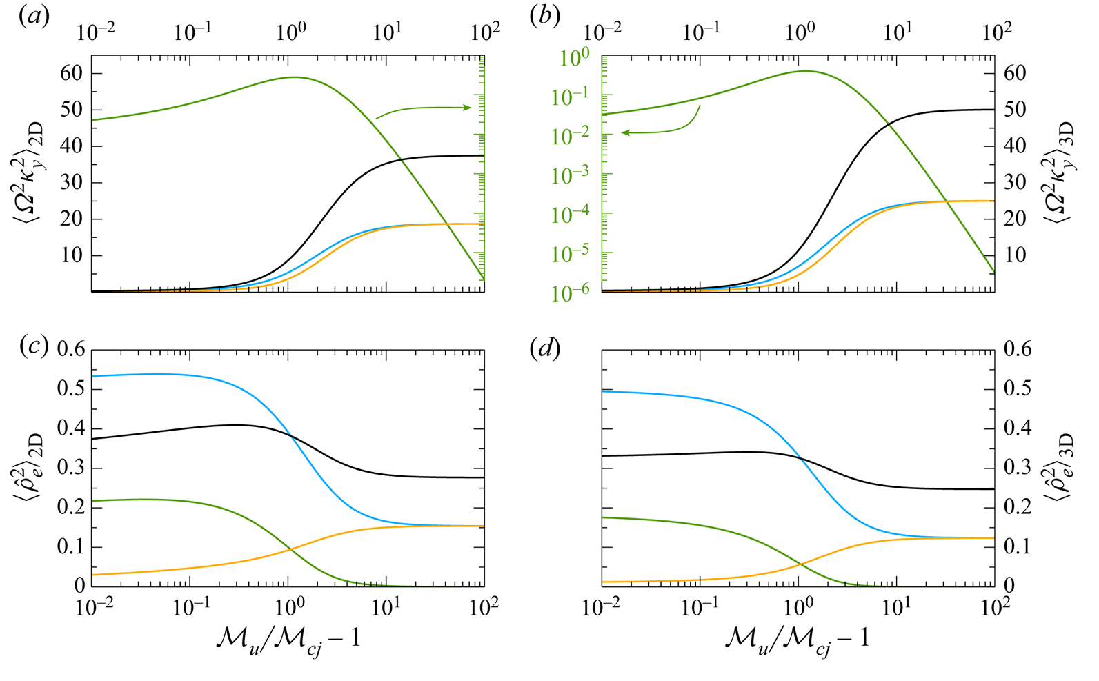
The averaged vorticity generated by the detonation front is computed in figure 5(a,b) in both two-dimensional (a) and three-dimensional (c) configurations as a function of the overdrive parameter $\mathcal {M}_u/\mathcal {M}_{cj}-1$. The amplification of the entropic density fluctuations is shown in figure 5(c,d). As noted for the turbulent kinetic energy, the highest level of vorticity generation is given when heat release perturbations upstream are negligible, i.e. when the mixture is in the heat release peak. This case, which is in black lines, is similar to that found in Huete et al. (Reference Huete, Sánchez and Williams2013). The opposite limit, which occurs for same-density gases in sufficiently rich or lean conditions, shows a peak in the enstrophy generation at finite degrees of overdrive ${\mathcal {M}}_u/{\mathcal {M}}_{cj}-1\sim 1$ (see the green curve with its own log–log scale). Expectedly, when heat release variations are comparable to density perturbations, negative correlations provide higher amplitudes for the vorticity perturbations downstream. It resembles the findings in Sinha (Reference Sinha2012), where the baroclinic torque due to a mean pressure gradient has an appreciable effect for non-zero entropic fluctuations in the upstream flow. As shown in figure 3, the highly overdriven limit for $|W|\gg |H|$ doubles the value for $|W|=|H|$.

Figure 5.

Averaged square vorticity (a,b) and square entropic density (c,d) in 2D (a and c) and 3D (b and d) geometries. Computations are shown as a function of the overdrive parameter $\mathcal {M}_u/\mathcal {M}_{cj}-1$ for $\gamma =1.2$, $Q = 1$, and $|W|\gg |H|$ (black lines), $|H|\gg |W|$ (green lines), $W=H$ (orange lines) and $W=-H$ (blue lines).

Regarding the change in the entropic heterogeneities due to the detonation passage (in terms of the dimensionless variables measured with the bulk density), it is observed that overdrive modifies the hierarchy of the dominant contributions in the generation of entropy. For weak overdrives, ${\mathcal {M}}_u/{\mathcal {M}}_{cj}-1\ll 1$, negative correlations render the highest levels of entropy, while positive correlations yield the lowest. For ${\mathcal {M}}_u/{\mathcal {M}}_{cj}\gg 1$, these contributions merge to the same asymptotic value, yielding half of that for $|W|\gg |H|$. The highest and lowest levels of entropy are obtained for $|W|\gg |H|$ and $|H|\gg |W|$, respectively, in the highly overdriven limit.

The results shown in figures 3–5 are qualitatively similar to those obtained previously for the interaction of detonations with random vorticity perturbations (Jackson et al. Reference Jackson, Hussaini and Ribner1993; Massa et al. Reference Massa, Chauhan and Lu2011; Massa & Lu Reference Massa and Lu2011; Huete et al. Reference Huete, Jin, Martínez-Ruiz and Luo2017). However, a detailed comparison requires taking into account the diverse criteria used for normalization in different investigations. For isotropic vorticity fields, the upstream perturbed velocity field was scaled in Jackson et al. (Reference Jackson, Hussaini and Ribner1993) and Huete et al. (Reference Huete, Jin, Martínez-Ruiz and Luo2017) with the speed of sound downstream from the detonation, which always increases with the detonation intensity. If it had been scaled with the upstream sound speed, the results would have shown how the downstream perturbations decay with the overdrive to become negligibly small for strongly overdriven detonations. In strong-shock conditions upstream perturbations in density and heat release will dominate the turbulence generation across the detonation wave. In this particular case, the turbulence amplification factors measure how much turbulence is generated for any convective perturbation of the fuel mass fraction of order $\epsilon /\sqrt {W^2+H^2}$. When $W$ and/or $H$ are large, the allowed fuel mass fraction perturbations must be much smaller than the corresponding density and/or heat release perturbations. This condition relaxes when $W$ and $H$ are of order unity or less. According to table 1, the value of $W$ is of order unity for light hydrocarbons and reasonably small for acetylene, while the value of $H$ is very sensitive to mixture conditions, being of order unity or less only in the vicinity of the heat release peak.

3.3. Turbulence scales characterization

Previous results refer to far-field mean values, which are independent of the shape of the energy spectrum, on condition that it is isotropic. The analysis is valid at a distance sufficiently far from the detonation wave, where the vanishing contribution of the acoustic energy can be neglected. Close to the detonation wave, however, the decaying pressure contribution should be taken into account as described in (A 18) in the appendix for monochromatic perturbations.

Near-field contributions are studied in detail in Sinha (Reference Sinha2012), Quadros, Sinha & Larsson (Reference Quadros, Sinha and Larsson2016) and Sethuraman, Sinha & Larsson (Reference Sethuraman, Sinha and Larsson2018) for inert shocks in canonical turbulent flows. To illustrate this effect, the emphasis is placed here on the near-field acoustic energy, which can be expressed as the sum of the non-vanishing and the vanishing contributions, namely $\langle \hat {p}^2\rangle ^{total}(x_s)=\langle \hat {p}^2\rangle ^{non\text {-}van} + \langle \hat {p}^2\rangle ^{van}(x_s)$, where $x_s = u_d t -x$ measures the distance from the detonation pointing backwards. The former, which is associated with high-frequency perturbations, is explicitly given in (3.9), while the decaying contribution is given by low-frequency disturbances in the form

(3.10)\begin{equation} \langle\hat{p}^2\rangle^{van}(x_s)= \frac{\displaystyle \int_0^\infty \left[\int_{\theta_c}^{{\rm \pi}/2} (\mathbb{P}_{l1}^2+\mathbb{P}_{l2}^2) \exp({-2\sigma(\theta)m k_o x_s})\sin\theta \,\textrm{d}\theta \right] \epsilon(m)^2 m^2\,\textrm{d}m}{\displaystyle \int_0^\infty \epsilon(m)^2 m^2\,\textrm{d}m} \end{equation}

for a three-dimensional isotropic spectrum $\epsilon (m)$ that is written in terms of the reduced wavenumber amplitude $m=k/k_o$. The function $\sigma (\theta )$, given in (A 19), defines the spatial decay rate along the dimensionless spatial coordinate $k_o x_s$. The decay rate depends on the form of the energy spectrum, which ultimately shapes the contribution of the different mode angles $\theta$.

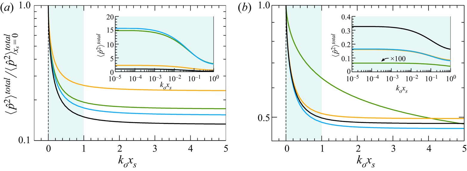
The reduced acoustic energy $\langle \hat {p}^2\rangle ^{total}/\langle \hat {p}^2\rangle ^{total}_{x_s=0}$ is shown in figure 6 as a function of the scaled distance $k_o x_s$. The functions are computed for $|W|\gg |H|$ (black lines), $|H|\gg |W|$ (green lines), $W=H$ (orange lines) and $W=-H$ (blue lines). Weakly overdriven detonations are displayed in panel (a) for $\mathcal {M}_u =1.001\mathcal {M}_{cj}$ and strongly overdriven detonations are shown in panel (b) for $\mathcal {M}_u =5\mathcal {M}_{cj}$. Except for the case $|H|\gg |W|$ in figure 6(b), which has been amplified by a factor of 100 in the inset, the decay rate is not significantly affected by the type of perturbation upstream. It takes a distance $x_s\sim k_o^{-1}$ for the acoustic energy to reach the asymptotic plateau corresponding to the far-field contribution. For weakly overdriven detonations, negative correlations exhibit the highest value of acoustic energy in the near field, in contrast to the far-field solution where perturbations of the type $|H|\gg |W|$ render slightly higher values. On the other hand, upstream flows dominated by density perturbations $|W|\gg |H|$ produce the highest acoustic energy in the whole spatial domain. In general, the vanishing contribution $\langle \hat {p}^2\rangle ^{van}$ has a relatively low influence on the total pressure field for $k_o x_s\gtrsim 1$. Note that near-field profiles are computed for purely inviscid flows. Depending on the particular conditions, there may exist another contribution coming from viscous dissipation that may not be neglected, as noted in Quadros et al. (Reference Quadros, Sinha and Larsson2016) and Sethuraman et al. (Reference Sethuraman, Sinha and Larsson2018).

Figure 6.

Three-dimensional total acoustic energy $\langle \hat {p}^2\rangle ^{total}/\langle \hat {p}^2\rangle ^{total}_{x_s=0}$ as a function of the scaled distance $k_o x_s$. Computations are given for $\gamma =1.2$, $Q = 1$, weakly overdriven detonations $\mathcal {M}_u = 1.001\mathcal {M}_{cj}$ (a), and strongly overdriven detonations $\mathcal {M}_u = 5\mathcal {M}_{cj}$ (b). The distinguished cases include $|W|\gg |H|$ (black lines), $|H|\gg |W|$ (green lines), $W=H$ (orange lines) and $W=-H$ (blue lines). The function $\langle \hat {p}^2\rangle ^{total}$ is shown in the insets for the same conditions.

To gain further insight into the properties of the turbulent flow that emerges far downstream of the detonation wave, the one-dimensional power spectra of the different variables can be evaluated through the integral functions

(3.11)\begin{gather} \varPhi_p(k_x) = N k_x^{-5/3}\int_0^{{\rm \pi}/2}\mathbb{P}^2(\theta) \frac{\sin^3\theta}{\cos^5\theta (k_x^{-2}+1+\tan^2\theta)^{17/6}}\textrm{d}\theta, \end{gather}

(3.12)\begin{gather}\varPhi_u(k_x) = N k_x^{-5/3}\int_0^{{\rm \pi}/2}\mathbb{U}^2(\theta) \frac{\sin^3\theta}{\cos^5\theta (k_x^{-2}+1+\tan^2\theta)^{17/6}}\textrm{d}\theta, \end{gather}

(3.13)\begin{gather}\varPhi_v(k_x) = N k_x^{-5/3}\int_0^{{\rm \pi}/2}\mathbb{V}^2(\theta) \frac{\sin^3\theta}{\cos^5\theta (k_x^{-2}+1+\tan^2\theta)^{17/6}}\textrm{d}\theta, \end{gather}

(3.14)\begin{gather}\varPhi_\rho(k_x) = N k_x^{-5/3}\int_0^{{\rm \pi}/2}\mathbb{D}^2(\theta)\frac{\sin^3\theta}{\cos^5\theta (k_x^{-2}+1+\tan^2\theta)^{17/6}} \textrm{d}\theta, \end{gather}

provided that the three-dimensional von Kármán model is applicable, as in Ribner (Reference Ribner1987) and Jackson et al. (Reference Jackson, Hussaini and Ribner1993), which translates into considering turbulence spectra of the form $\epsilon (k_x,k_y)^2 \sim k_y^2/(1+k_x^2+k_y^2)^{17/6}$. The normalization parameter is chosen to satisfy

(3.15)\begin{equation} N^{-1} = \int_{-\infty}^{\infty}\int_0^{\infty} \frac{k_y^2}{(1+k_x^2+k_y^2)^{17/6}} k_y\,\textrm{d}k_y \,\textrm{d}k_x. \end{equation}

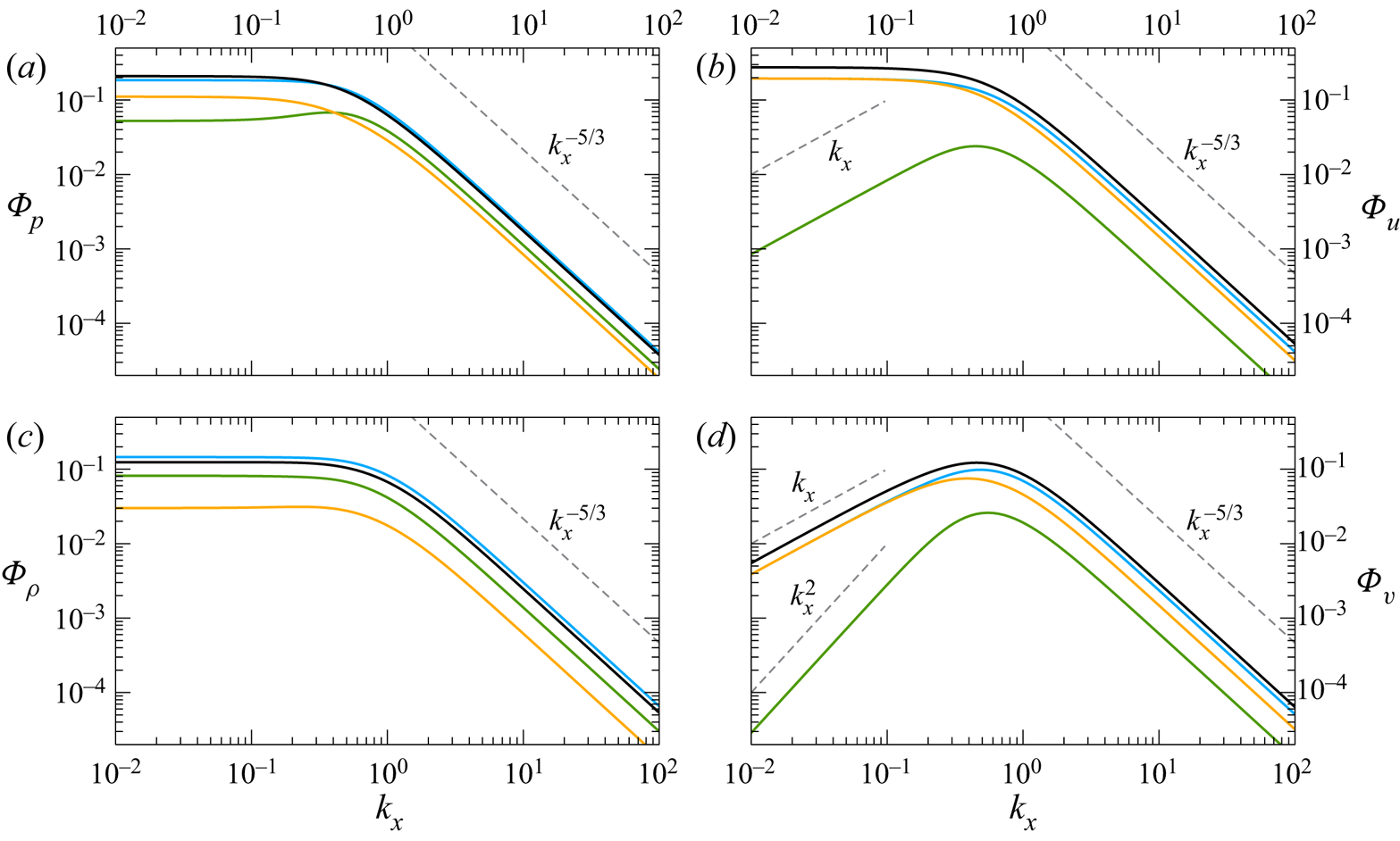
Previous investigations on the interaction of turbulence with adiabatic shocks have reported that large-scale turbulence is amplified to a greater extent than small-scale motions (Andreopoulos, Agui & Briassulis Reference Andreopoulos, Agui and Briassulis2000). A similar behaviour is observed with detonations when they travel in isotropic vorticity flows (Jackson et al. Reference Jackson, Hussaini and Ribner1993) or isotropic entropic density flows, as the example considered here for $|W|\gg |H|$. This phenomenon is readily observed in the black curves plotted in figure 7, where the power spectra $\varPhi _p$, $\varPhi _u$, $\varPhi _v$ and $\varPhi _\rho$ are represented as a function of the longitudinal wavenumber $k_x$ for $\gamma =1.2$, $\mathcal {M}_u = 1.2\mathcal {M}_{cj}$, $Q = 1$, and for $|W|\gg |H|$ (black lines), $|H|\gg |W|$ (green lines), $W=H$ (orange lines) and $W=-H$ (blue lines). In the presence of upstream density perturbations $W$ with values of $H$ that are either negligible or of the same order, the curves exhibit a similar pattern, and the case $|W|\gg |H|$ results in the highest values along with the negatively correlated cases $W=-H$. As a result of the destructive interference, positive correlations yield lower values in most of the domains for each spectrum. The case $|H|\gg |W|$ results in the lowest intensity for the two velocity spectra in all the domains and for the pressure spectrum for small wavenumbers only. Regarding this large-scale limit, it is noticeable that curves of $\varPhi _u$ approach a plateau as $k_x$ decreases except for the case $|H|\gg |W|$, where the spectrum decreases as $k_x^{-1}$. Curves for $\varPhi _v$ decrease as $k_x$ is reduced in all cases; however, the isochoric case shows a higher slope $k_x^{-2}$. Regarding $\varPhi _p$ and $\varPhi _\rho$, they reach plateaus in the large-scale limit for any combination of $W$ and $H$. With respect to the small-scale regime, all contributions obey the von Kármán decay law $k_x^{-5/3}$. Although these conclusions apply for $\mathcal {M}_u = 1.2\mathcal {M}_{cj}$, they can be extrapolated to higher overdrives. On the other hand, the weakly overdriven limit should be discussed separately, as the acoustic part may change the ranking of the most important contributions.

Figure 7.

One-dimensional power spectra of the pressure (a), density (c) and longitudinal and transverse velocity components (b and d, respectively). Computations are shown as a function of the wavenumber $k_x$ for $\gamma =1.2$, $\mathcal {M}_u = 1.2\mathcal {M}_{cj}$, $Q = 1$, and $|W|\gg |H|$ (black line), $|H|\gg |W|$ (green lines), $W=H$ (orange lines) and $W=-H$ (blue lines).

Aside from the fact that viscosity and molecular diffusion are not accounted for in the model – in which case the spectra would become time-dependent functions after the passage of the detonation (Sinha Reference Sinha2012; Sethuraman & Sinha Reference Sethuraman and Sinha2020), the small-scale regime must be taken with caution as the thin-detonation hypothesis may not be fulfilled. Therefore, the properties of the turbulent flow behind the detonation front predicted by the linear interaction theory should be further extended to include the effects of finite reaction lengths, as noted in Massa et al. (Reference Massa, Chauhan and Lu2011) and Massa & Lu (Reference Massa and Lu2011), and nonlinear contributions, as noted in Larsson & Lele (Reference Larsson and Lele2009), Prakash & Raman (Reference Prakash and Raman2019), Livescu (Reference Livescu2020) and Tian et al. (Reference Tian, Jaberi and Livescu2020). The latter is unavoidable if multi-phase environments are under consideration (Watanabe et al. Reference Watanabe, Matsuo, Matsuoka, Kawasaki and Kasahara2019, Reference Watanabe, Matsuo, Chinnayya, Matsuoka, Kawasaki and Kasahara2020). However, there are some aspects predicted by the model that deserve particular attention. When a detonation wave or a reactive shock is considered, the possibility of having different heat releases across the detonation wave due to non-perfect mixing should not be neglected. This effect plays a leading role in the turbulence generation process of acoustic type in the CJ condition. As a result, the turbulent flow downstream cannot be assumed to be isobaric, as reasonably done for inert shocks. For detonations, the dilatational part of the velocity gradient tensor cannot be neglected when the correlations between the corresponding invariants are employed to characterize the topology of the turbulent flow.

4.1. Averaged turbulent Rankine–Hugoniot jump equations

The changes in the RH relations are given by second-order corrections in the form

(4.2a–c)\begin{align} \frac{\langle\rho_d\rangle}{\langle\rho_u\rangle} = {\mathcal{R}}_d (1+\bar{\epsilon}^2 \delta {\mathcal{R}}),\quad \frac{\langle p_d\rangle}{p_u} = {\mathcal{P}}_d (1+\bar{\epsilon}^2 \delta {\mathcal{P}} ),\quad \frac{\langle u_d\rangle}{u_u} = \dfrac{1}{{\mathcal{R}}_d} (1+\bar{\epsilon}^2 \delta {\mathcal{U}}), \end{align}

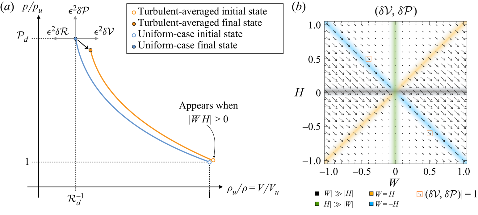
provided that the flow perturbations can be written as the breakdown of averaged and local deviation contributions, e.g. $\rho _d=\langle \rho _d\rangle (1+\bar {\epsilon }\hat {\rho } )$ for the burnt-gas density field. To illustrate this, figure 8(a) sketches the effect of the second-order corrections to the post-detonation RH values. Hollow circles represent the initial conditions, which may also be different if second-order average values are non-zero. The blue and orange filled circles indicate the one-dimensional and turbulent post-detonation conditions, respectively. The vector $(\delta \mathcal {V}, \delta \mathcal {P})$, with $\delta \mathcal {V}=-\delta \mathcal {R}$ standing for the correction to the specific volume, is defined to characterize the relative deviations of the post-detonation RH state on the $(V/V_u,p/p_u)$-plane. Figure 9(b) shows the vector $(\delta \mathcal {V}, \delta \mathcal {P})$ as computed from the theory presented below for the same conditions given in figure 9, namely, $\gamma =1.2$, $\mathcal {M}_u = 1.2\mathcal {M}_{cj}$ and $Q = 1$. In this case, both pressure and density corrections are negative in the whole domain, yet the values differ significantly depending on the particular values of $W$ and $H$. Note also that in agreement with the results of § 3, perturbations weaken for $|H|\gg W$ and intensify for $|H|\ll W$.

Figure 8.

(a) Sketch for the Rankine–Hugoniot curves. In blue the one-dimensional curve and in orange the second-order averaged curve. (b) Computations for $\gamma =1.2$, $\mathcal {M}_u = 1.2\mathcal {M}_{cj}$, $Q = 1$, $H = [-1\!:\!1]$ and $W = [-1\!:\!1]$.

Figure 9.

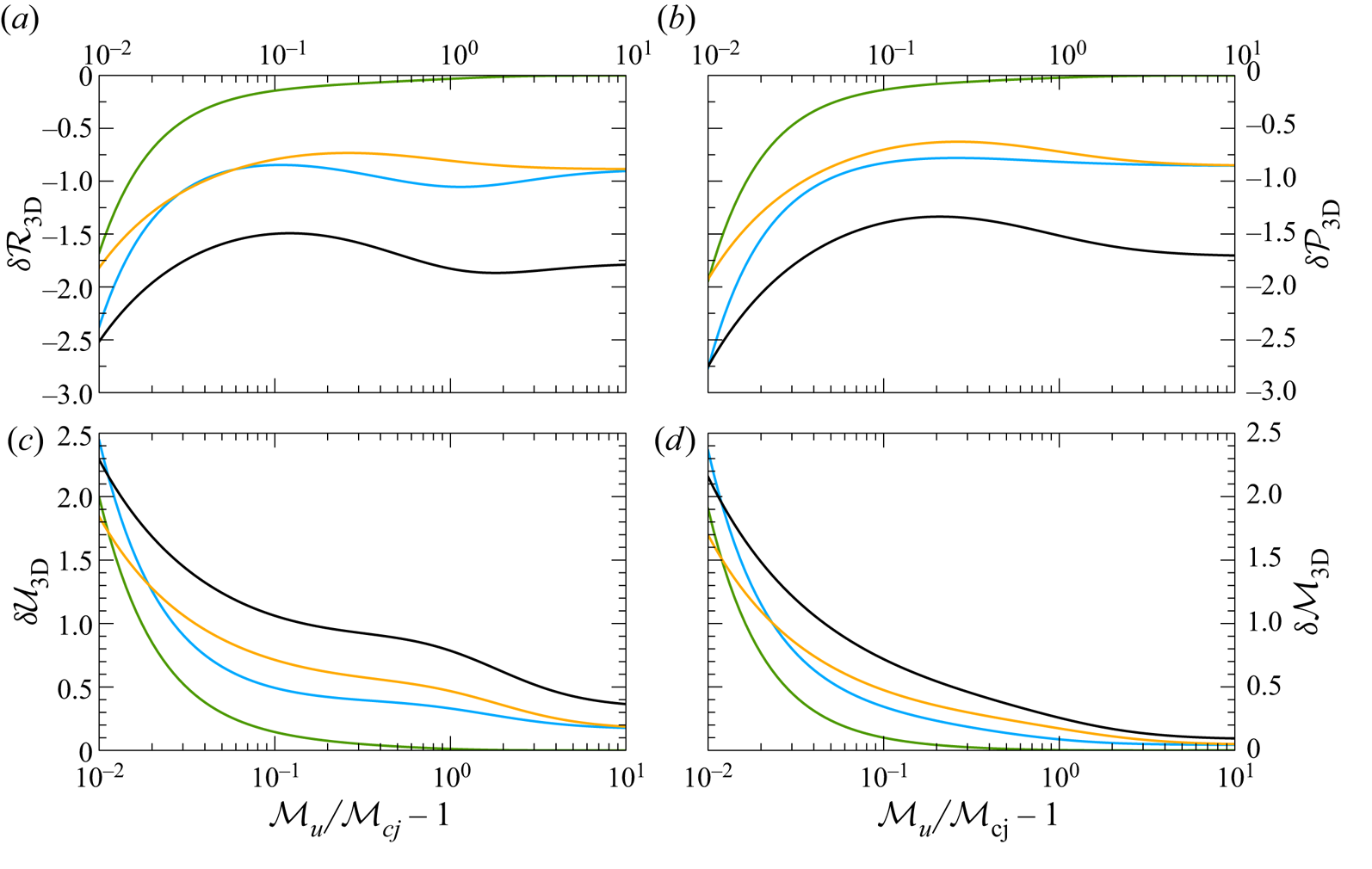
Three-dimensional second-order correction to the RH jump conditions (a) $\delta \mathcal {R}$, (b) $\delta \mathcal {U}$, (c) $\delta \mathcal {P}$ and (d) $\delta \mathcal {M}$ as a function of the overdrive parameter $\mathcal {M}_u/\mathcal {M}_{cj}-1$. Computations correspond to $\gamma =1.2$, $Q = 1$, and $|W|\gg |H|$ (black lines), $|H|\gg |W|$ (green lines), $W=H$ (orange lines) and $W=-H$ (blue lines).

Corrections to the RH jump conditions due to weak turbulence are derived from the lowest non-vanishing order, i.e. the nonlinear second-order terms describing the interaction between the different perturbation modes and their self-interactions. The natures of rotational and entropic modes are similar as they are both carried along with the fluid. Thus, they correlate and provide rotational–entropic and rotational–rotational second-order corrections. By contrast, acoustic waves are uncorrelated with the entropic and rotational perturbations. As a consequence, second-order corrections can be decomposed into entropic–rotational and acoustic–acoustic terms, separately.

The entropic–rotational correlations enter only as second-order corrections as the first order of the random-phase oscillating terms vanishes. Conversely, acoustic perturbations play a two-fold role in the global contribution. The first role, which is akin to entropic–rotational modes, is given by second-order corrections to the mass, momentum and energy fluxes across the detonation front. The second role stems from the fact that acoustic waves shift the average values of the flow variables in the second order of the sound amplitude. Further details of the analytical derivation of the distinguished contributions can be withdrawn from Velikovich et al. (Reference Velikovich, Huete and Wouchuk2012) and references therein, particularly the supplemental material, as well as in Westervelt (Reference Westervelt1950), Blackstock (Reference Blackstock1962) and Ostrovskii (Reference Ostrovskii1968).

As a result of the second-order corrections to the mass, momentum and energy fluxes across the detonation wave, the downstream pressure, density and streamwise velocity suffer the corresponding corrections $\delta \mathcal {P}_{f}$, $\delta \mathcal {R}_{f}$ and $\delta \mathcal {U}_{f}$, where the subscript ${f}$ is used to denote changes due to flux corrections. These corrections can be obtained from the averaged turbulent conservation equations, namely

(4.3a)\begin{gather} \langle \rho_u u_u \rangle = \langle \rho_d u_d \rangle, \end{gather}

(4.3b)\begin{gather}\langle p_u + \rho_u u_u^2 \rangle = \langle p_d +\rho_d u_d^2 \rangle, \end{gather}

(4.3c)\begin{gather}\left\langle \frac{\gamma}{\gamma-1}p_u u_u + \frac{1}{2}\rho_u u_u^3 + \rho_u u_u q_u \right\rangle = \left\langle \frac{\gamma}{\gamma-1}p_d u_d + \frac{1}{2}\rho_d u_d \left(u_d^2+v_d^2\right) \right\rangle, \end{gather}

which provide, with use made of (4.2a–c) and knowing that first-order entropic and rotational corrections give null average contributions, the second-order relationships

(4.4a)\begin{gather} \delta\mathcal{R}_{f} + \delta\mathcal{U}_{f} + {\mathcal{M}}_d^{-1}\langle l_{f} \rangle = 0, \end{gather}

(4.4b)\begin{gather}\delta\mathcal{P}_{f} + \gamma\mathcal{M}_d^2(\delta\mathcal{R}_{f}+2 \delta\mathcal{U}_{f}) + \gamma\langle m_{f} \rangle= 0, \end{gather}

(4.4c)\begin{gather}\mathcal{M}_d^2 \delta\mathcal{R}_{f}+ \left(3\mathcal{M}_d^2 + \frac{2}{\gamma-1}\right) \delta\mathcal{U}_{f} + \frac{2}{\gamma-1} \delta\mathcal{P}_{f} + \frac{2}{(\gamma-1)\mathcal{M}_d}\langle n_{f}\rangle = q_{wh}, \end{gather}

where the factor

(4.5)\begin{equation} q_{wh}=\frac{4 Q \mathcal{M}_d^2 \mathcal{R}_d^2}{(\gamma^2-1)\mathcal{M}_u^2} \langle \hat{\rho}_u \hat{q}_u \rangle=\frac{4 Q \mathcal{R}_d}{(\gamma^2-1)\mathcal{P}_d} \frac{W H}{W^2 + H^2} \end{equation}

appears due to the existence of two non-vanishing second-order sources of perturbations upstream. The factor $q_{wh}$ vanishes for flows with uniform density or constant heat release given that first-order averages of entropic disturbances do not provide net contributions. The terms $\langle l_{f} \rangle$, $\langle m_{f} \rangle$ and $\langle n_{f} \rangle$ represent the dimensionless second-order turbulent corrections to the mass, streamwise momentum and energy fluxes, respectively. As mentioned above, the terms split into entropic–rotational (subscript $er$) and acoustic–acoustic (subscript $aa$) contributions to yield

(4.6a)\begin{gather} \langle l_{f} \rangle = \langle l_{er} \rangle +\langle l_{aa} \rangle = \langle \hat{\rho}_e \hat{u}_r\rangle -\frac{\gamma+1}{4}{\mathcal{M}}_d\langle \hat{p}^2\rangle, \end{gather}

(4.6b)\begin{gather}\langle m_{f} \rangle = \langle m_{er} \rangle +\langle m_{aa} \rangle = 2\mathcal{M}_d \langle \hat{\rho}_e\hat{u}_r\rangle + \langle \hat{u}_r^2\rangle -\frac{(\gamma-1)\mathcal{M}_d^2+3-\gamma}{4} \langle\hat{p}^2\rangle+ \langle \hat{u}_a^2\rangle, \end{gather}

(4.6c)\begin{align} \langle n_{f} \rangle &= \langle n_{er} \rangle +\langle n_{aa} \rangle = \frac{{\mathcal{M}}_d(\gamma-1)}{2} \left[3 \langle \hat{u}_r^2\rangle+ \langle \hat{v}_r^2\rangle+3{\mathcal{M}}_d\langle \tilde{\rho}_e \tilde{u}_r\rangle\right] \nonumber\\ &\quad -\frac{(\gamma+1){\mathcal{M}}_d}{8}\left[(\gamma-1){\mathcal{M}}_d^2+2(2-\gamma)\right] \langle\hat{p}^2\rangle +(\gamma-1){\mathcal{M}}_d \langle \hat{u}_a^2\rangle \nonumber\\ &\quad -(\gamma-1)\langle\hat{p}\hat{u}_a\rangle, \end{align}

where $\langle \hat {u}_r^2\rangle$, $\langle \hat {u}_a^2\rangle$, $\langle \hat {v}_r^2\rangle$ and $\langle \hat {p}^2\rangle$ have been previously defined in (3.5), (3.6) and (3.9). The averages $\langle \tilde {\rho }_e \tilde {u}_r\rangle$ and $\langle \hat {p}\hat {u}_a\rangle =\langle \hat {\rho }_a\hat {u}_a\rangle$ are second-order contributions that have not been previously introduced. As noted in (3.5), (3.6) and (3.9), these parameters can be written in terms of integral expressions for two-dimensional and three-dimensional upstream isotropic spectra, namely

(4.7)\begin{equation} \left.\begin{gathered} \langle \hat{\rho}_e \hat{u}_r \rangle_{2D} = - \frac{2}{\rm \pi}\int_0^{\theta_c}\mathbb{D}_{e,h} \mathbb{U}_{r,h}\,\textrm{d} \theta-\frac{2}{\rm \pi}\int_{\theta_c}^{{\rm \pi}/2}\left[\mathbb{D}_{e,l1} \mathbb{U}_{r,l1}+\mathbb{D}_{e,l2} \mathbb{U}_{r,l2}\right] \textrm{d} \theta, \\ \langle \hat{\rho}_e \hat{u}_r \rangle_\textrm{3D} = -\int_0^{\theta_c} \mathbb{D}_{e,h} \mathbb{U}_{r,h} \sin\theta\,\textrm{d} \theta - \int_{\theta_c}^{{\rm \pi}/2}\left[\mathbb{D}_{e,l1} \mathbb{U}_{r,l1}+\mathbb{D}_{e,l2} \mathbb{U}_{r,l2}\right]\sin\theta\,\textrm{d} \theta, \end{gathered}\right\} \end{equation}

and

(4.8a,b)\begin{equation} \langle\hat{p}\hat{u}_a\rangle_\textrm{2D} =\frac{2}{\rm \pi}\int_0^{\theta_c}\mathbb{P}_h\mathbb{U}_a\ \textrm{d} \theta,\quad \langle\hat{p}\hat{u}_a\rangle_\textrm{3D} =\int_0^{\theta_c}\mathbb{P}_h\mathbb{U}_a\sin\theta\ \textrm{d} \theta \end{equation}

for the entropic–rotational contribution to the mass flux and the projected acoustic contribution to the energy flux, respectively. The amplitudes of the entropic density and the rotational streamwise velocity are given in (A 22) and (A 29), respectively, and the negative sign arises from the opposite direction between the flow and the orientation of the detonation front. Finally, the amplitude of the pressure perturbations $\mathbb {P}_h$ together with $\mathbb {U}_a=\mathbb {P}_{h} \kappa _a/\omega _a$ is given in (A 9). It is readily observed that $\langle \hat {\rho }_e \hat {u}_r \rangle$ is directly associated to the far-field convective energy flux, which is studied in detailed in Quadros et al. (Reference Quadros, Sinha and Larsson2016) and Sethuraman et al. (Reference Sethuraman, Sinha and Larsson2018) for different types of spectra in canonical shock-turbulence scenarios.

The post-shock density, pressure and streamwise velocity component exhibit second-order changes due to the presence of the acoustic wave field. The dual temporal-spatial averaging that is conveniently applied to this problem is similar to time averaging performed in the reference frame with the gas at rest. The averaging must be computed in the Eulerian reference system at a fixed position relative to the detonation front. Therefore, as a direct consequence of the shift in the acoustic waves, there exists an additional contribution in the burnt-gas properties, namely

(4.9a–c)\begin{equation} \delta\mathcal{R}_{b} = - \frac{\gamma+1}{4}\langle \hat{p}^2\rangle,\quad \delta\mathcal{P}_{b} = -\frac{\gamma(3-\gamma)}{4}\langle \hat{p}^2\rangle,\quad \delta\mathcal{U}_{b} = \frac{1}{\mathcal{M}_d}\langle \hat{p}\hat{u}_a\rangle, \end{equation}

where the subscript ${b}$ denotes changes in the background downstream properties due to random-phase acoustic perturbations. The ultimate corrections to the RH jump conditions are given by the sum of the contributions due to the turbulent fluxes (subscript $f$) and background corrections induced by the acoustic field (subscript $b$). With use made of (4.4), (4.6) and (4.9a–c), the turbulent corrections to the RH conditions read as follows:

(4.10)\begin{align} \delta \mathcal{R} &= \delta\mathcal{R}_{f} + \delta\mathcal{R}_{b} = \frac{1}{1-\mathcal{M}^2_d}\left[\frac{\mathcal{M}_d^2(\gamma+3)-2}{2\mathcal{M}_d}\langle l_{f}\rangle - \gamma\langle m_{f}\rangle +\frac{1}{\mathcal{M}_d}\langle n_{f}\rangle- \frac{\gamma-1}{2}q_{wh}\right] \nonumber\\ &\quad -\frac{\gamma+1}{4}\langle \hat{p}^2\rangle, \end{align}

(4.11)\begin{align} \delta \mathcal{P} &= \delta\mathcal{P}_{f} + \delta\mathcal{P}_{b} = \frac{\gamma}{1-\mathcal{M}^2_d} \left[\frac{\mathcal{M}_d [\mathcal{M}_d^2(\gamma-1)+2]}{2}\langle l_{f}\rangle - [\mathcal{M}_d^2(\gamma-1)+1]\langle m_{f}\rangle \right. \nonumber\\ &\quad \left.\vphantom{\frac{\mathcal{M}_d\left[\mathcal{M}_d^2(\gamma-1)+2\right]}{2}} +\mathcal{M}_d\langle n_{f}\rangle - \frac{\mathcal{M}_d^2(\gamma-1)}{2}q_{wh} \right] -\frac{\gamma(3-\gamma)}{4}\langle \hat{p}^2\rangle, \end{align}

(4.12)\begin{align} \delta \mathcal{U} &= \delta\mathcal{U}_{f} + \delta\mathcal{U}_{b} = \frac{-1}{1-\mathcal{M}^2_d}\left[\frac{\mathcal{M}_d(\gamma+1)}{2}\langle l_{f}\rangle - \gamma\langle m_{f}\rangle +\frac{1}{\mathcal{M}_d}\langle n_{f}\rangle- \frac{\gamma-1}{2}q_{wh}\right] \nonumber\\ &\quad + \frac{1}{\mathcal{M}_d}\langle \hat{p}\hat{u}_a\rangle. \end{align}

Associated to the turbulence-induced changes in the RH jump conditions, the Mach number of the burnt-gas fluid particles is also modified according to

(4.13)\begin{equation} \delta \mathcal{M}=\frac{\mathcal{M}_u}{\sqrt{\mathcal{R}_d \mathcal{P}_d}} \left(\delta \mathcal{U}+\frac{1}{2}\delta \mathcal{R}-\frac{1}{2}\delta \mathcal{P}\right). \end{equation}

Computations of $\delta \mathcal {R}$, $\delta \mathcal {P}$, $\delta \mathcal {U}$ and $\delta \mathcal {M}$ are represented in figure 9 as a function of the overdrive parameter $\mathcal {M}_u /\mathcal {M}_{cj}-1$ for three-dimensional isotropic perturbations with $\gamma =1.2$ and $Q = 1$. The four distinguished cases include $|W|\gg |H|$ (black lines), $|H|\gg |W|$ (green lines), $W=H$ (orange lines) and $W=-H$ (blue lines). Density and pressure corrections, $\delta \mathcal {R}$ and $\delta \mathcal {P}$, are always negative, and the amplitude of the second-order corrections weakens with the overdrive and approaches an asymptotic constant value that is null only when $W=0$, which is consistent with previous turbulence generation functions. 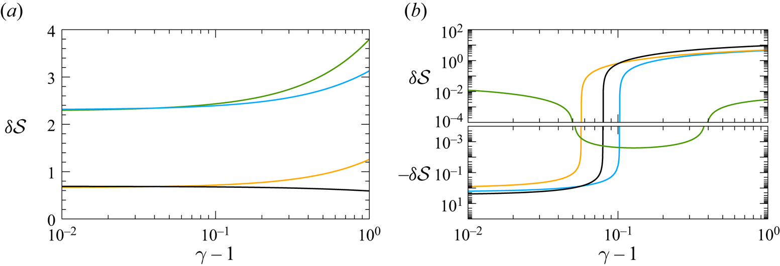A qualitative representation of the combined effect of $\delta \mathcal {P}$ and $\delta \mathcal {R}$ is shown in figure 8(b) in terms of the vector $(\delta \mathcal {V}, \delta \mathcal {P})$, with $\delta \mathcal {V}=-\delta \mathcal {R}$. Curves of the post-detonation velocity and corresponding Mach number go in the opposite direction because $\delta \mathcal {U}$ and $\delta \mathcal {M}$ exhibit positive values in all cases. For the conditions chosen in figure 9, perturbations involving only density changes result in the strongest corrections, while those involving only variations in heat release yield the weakest corrections far from the CJ condition. Positive and negative correlations, on the other hand, yield intermediate values for the second-order corrections.

4.2. Detonation propagation speed

The averaged turbulent properties of the post-detonation state differ from those of the unperturbed, i.e. one-dimensional case. Second-order corrections for density, pressure and velocity must be accounted for to properly describe the burnt-gas state. In real conditions, depending on the experimental set-up, boundary conditions may impose different restrictions to the burnt-gas flow. For example, a highly overdriven detonation formed by a piston-driven shock travelling into the reactive mixture forces the velocity of the burnt-gas particles to be equal to the piston velocity, $u_p=u_u-u_d$, in steady state. Then, along with the velocity variation of the expelled burnt gas $\delta \mathcal {U}$, a detonation propagation speed correction must occur to satisfy the boundary condition, i.e. $\delta \langle u_p\rangle =0=\delta u_u- \bar {\epsilon }^2 u_d \delta \mathcal {U}$, which yields

(4.14)\begin{equation} \left.\delta {\mathcal{S}}\right|_{\delta\langle u_p\rangle=0}= \frac{1}{\bar{\epsilon}^2}\left. \frac{\delta u_u}{u_u}\right|_{\delta\langle u_p\rangle=0}= \frac{1}{\mathcal{R}_d}\delta \mathcal{U}, \end{equation}

where $\delta {\mathcal {S}}$ is an order-of-unity function that characterizes the correction of the detonation propagation speed. According to the results shown in figure 9, where $\delta \mathcal {U}$ is positive, the accommodated velocity of the detonation is therefore increased. Except for weakly overdriven detonations, where negative correlated perturbations $W=-H$ render the strongest correction, the case corresponding to dominant density perturbations $W\gg H$ is the case where the detonation would move faster compared to the homogeneous case.

Another canonical possibility is that total pressure (including corrections) must remain invariant. For this to be true, $\delta \langle p_d\rangle =0=p_d \bar {\epsilon }^2 \delta \mathcal {P}+(\textrm {d}p_d)/(\textrm {d}u_u)\delta u_u$ and the detonation propagation speed must be adapted according to

(4.15)\begin{equation} \left.\delta {\mathcal{S}}\right|_{\delta\langle p_d\rangle=0}= \frac{1}{\bar{\epsilon}^2}\left. \frac{\delta u_u}{u_u}\right|_{\delta\langle p_d\rangle=0}=- \frac{\mathcal{P}_d}{\mathcal{M}_u}\left(\frac{\textrm{d}\mathcal{P}_d}{\textrm{d}\mathcal{M}_u}\right)^{-1}\delta \mathcal{P}, \end{equation}

where $(\textrm {d}\mathcal {P}_d)/(\textrm {d}\mathcal {M}_u)>0$ and $\delta \mathcal {P}<0$, according to figure 9. Then, the constant-pressure boundary condition also predicts a positive second-order correction to the propagation speed, which aligns with the previous boundary condition. These considerations oppose the initially imposed isolated-wave boundary condition. For (4.14) and (4.15) to be true along with the isolated condition, the influence of the coupling surface must be sufficiently far away from the detonation for the asymptotic oscillating regime to be achieved before the reflections come into play. Certainly, more complex scenarios may require non-canonical boundary conditions to be imposed. For example, for a detonation moving along a tube with the back extreme being open, the boundary condition should be given by the corresponding matching of the far-field non-reflective condition with the acoustics inside the channel because both velocity and pressure variations are non-zero $\delta \langle u_p\rangle \neq \delta \langle p_d\rangle \neq 0$ downstream.

Regarding detonations travelling close to the CJ velocity, $1-\mathcal {M}_d\ll 1$, the closure is given by imposing $\delta \langle \mathcal {M}_d\rangle =0$, i.e. not admitting variations in the post-detonation Mach number as the reacting gas expands up to its maximum value $\mathcal {M}_d=1$. Since the corresponding second-order correction to the RH conditions predicts variations in the flow velocity $u_d$ and in the speed of sound $a_d$, the detonation propagation velocity must provide $\delta \langle \mathcal {M}_d\rangle =0= \bar {\epsilon }^2 \delta \mathcal {M}+(\textrm {d}\mathcal {M}_d)/(\textrm {d}u_u)\delta u_u$, and then

(4.16)\begin{equation} \left.\delta {\mathcal{S}}\right|_{\delta\langle \mathcal{M}_d\rangle=0}= \frac{1}{\bar{\epsilon}^2}\left. \frac{\delta u_u}{u_u}\right|_{\delta\langle \mathcal{M}_d\rangle=0}=- \frac{1}{\sqrt{\mathcal{R}_d \mathcal{P}_d}}\left(\frac{\textrm{d}\mathcal{M}_d}{\textrm{d}\mathcal{M}_u}\right)^{-1} \left(\delta \mathcal{U}+\frac{1}{2}\delta \mathcal{R}-\frac{1}{2}\delta \mathcal{P}\right). \end{equation}

The variation of the propagation speed is studied through the order-of-unity factor $\delta {\mathcal {S}}$ as a function of the overdrive $\mathcal {M}_u/\mathcal {M}_{cj}-1$, reduced heat release $\tilde {Q}$ and specific heat ratio $\gamma$ in figures 10, 11 and 12, respectively. To properly isolate the effects, heat release is conveniently redefined with the thermal enthalpy upstream $\tilde {Q}=q_u/(c_{p_u} T_u)$, which relates to $Q=\tilde {Q} (\gamma +1)/2$ in the former definition.

Figure 10.

Three-dimensional second-order correction of the detonation propagation velocity $\delta \mathcal {S}$, according to (4.16), as a function of the overdrive parameter $\mathcal {M}_u/\mathcal {M}_{cj}-1$. Computations are provided for $\gamma = 1.2$, $\tilde {Q} = 1$ (a) and $\tilde {Q} = 10$ (b) evaluated for $|W|\gg |H|$ (black lines), $|H|\gg |W|$ (green lines), $W=H$ (orange lines) and $W=-H$ (blue lines).

Figure 11.

Three-dimensional second-order correction of the detonation propagation velocity $\delta \mathcal {S}$, according to (4.16), as a function of the dimensionless heat release $\tilde {Q}$. Computations are shown for $\gamma = 1.2$, weak overdrives as $\mathcal {M}_u = 1.001\mathcal {M}{cj}$ (a) and strong overdrives as $\mathcal {M}_u = 5\mathcal {M}{cj}$ (b). $|W|\gg |H|$ (black lines), $|H|\gg |W|$ (green lines), $W=H$ (orange lines) and $W=-H$ (blue lines).

Figure 12.

Three-dimensional second-order correction of the detonation propagation velocity $\delta \mathcal {S}$, according to (4.16), as a function of the adiabatic constant as $\gamma -1$. Computations are given for $\tilde {Q} = 1$, weak overdrives as $\mathcal {M}_u = 1.001\mathcal {M}{cj}$ (a) and strong overdrives as $\mathcal {M}_u = 5\mathcal {M}{cj}$ (b). Computations are evaluated for $|W|\gg |H|$ (black lines), $|H|\gg |W|$ (green lines), $W=H$ (orange lines) and $W=-H$ (blue lines).

Figure 10 shows the variation of the detonation propagation velocity given by (4.16) as a function of $\mathcal {M}_u/\mathcal {M}_{cj}-1$ for three-dimensional isotropic perturbations, $\gamma =1.2$, $\tilde {Q} = 1$ (a) and $\tilde {Q} = 10$ (b). The four distinguished cases include $|W|\gg |H|$ (black lines), $|H|\gg |W|$ (green lines), $W=H$ (orange lines) and $W=-H$ (blue lines). For strongly overdriven detonations, dominant density perturbations induce the highest amplification to the propagation velocity. For iso-density mixtures, $|H|\gg |W|$ the correction of the propagation speed becomes negative for sufficiently overdriven detonations, thereby resulting in a slower propagation speed. However, this effect can be effectively neglected in view of its amplitude. Increasing the value of $\tilde {Q}$ results in higher values of $\delta {\mathcal {S}}$ for weakly overdriven detonations, except for $|W|\gg |H|$. Weakly overdriven detonations are dominated by heat release perturbations, where the case $|H|\gg |W|$ predicts the highest amplification.

The effect of heat release is better analysed in figure 11, where the function $\delta {\mathcal {S}}$ is computed as a function of $\tilde {Q}$ for weakly overdriven (a) and strongly overdriven (b) detonations. Figure 11(a) shows that weakly overdriven detonations in a heterogeneous mixture tend to move faster for any value of $\tilde {Q}$. Regarding the type of mixture, higher heat release is associated with smaller amplification for $|W|\gg |H|$, while the opposite is found for $|H|\gg |W|$. Intermediate mixture properties $W = H$ and $W = -H$ present in-between values. For strongly overdriven detonations (b), the effect of heat release is to amplify the propagation speed when density perturbations are not negligible. However, a negative correction is found for iso-density mixtures dominated by heat release perturbations $|H|\gg |W|$; however, the order of magnitude, which is significantly smaller, predicts a negligible correction to the propagation speed.

The effect of the specific heats ratio $\gamma$ is displayed in figure 12, where the factor $\delta {\mathcal {S}}$ is computed as a function of $\gamma -1$ for weakly overdriven (a) and strongly overdriven (b) detonations. The former, in agreement with previous figures, shows an always positive velocity correction. When density perturbations dominate the upstream flow, the reduction of $\gamma$ results in a higher propagation speed, but this trend reverses when heat release perturbations are included. Overdriven detonations, on the other hand, exhibit a less intuitive picture. For values of $\gamma$ between 1.1 and 1.4, the cases of utmost interest, results are qualitatively similar to those obtained previously for $\gamma =1.2$, where the case $|H|\gg |W|$ predicts minor negative corrections to the propagation speed, and the cases $|W|\gg |H|$ and $|W|=|H|$ predict positive order-of-unity values of $\delta {\mathcal {S}}$.

Based on the analysis performed in the previous section, where the relative weight of the different type of perturbations in the burnt gas has been computed, it can be concluded that CJ-detonations moving in heterogeneous mixtures are governed by acoustic-type turbulent fluctuations in the burnt gas when net heat release is not negligible. Consequently, these factors are highly influenced by the heat release variations derived from the upstream heterogeneities with the correlation with density perturbations playing a dominant role in the formation of turbulent structures downstream. These results are in qualitative agreement with previous numerical simulations (Mi et al. Reference Mi, Higgins, Ng, Kiyanda and Nikiforakis2017a,Reference Mi, Timofeev and Higginsb); however, the numerical set-up is not completely compatible with the assumptions made in this theoretical model. Spatial inhomogeneities are introduced by collecting the energy sources into discretized reactive layers and into reactive square-based prisms, both of which are spatially separated by inert regions ($\bar {\epsilon }\sim 1$). They found that the average wave propagation velocity is greater, up to 10 %, than the CJ velocity of the equivalent homogeneous medium when the characteristic scale of the perturbations is greater than the inherent reaction zone length. The wave in CJ conditions speeds up when the specific heat ratio decreases. In agreement with linear theory, when the amplitude of the upstream heterogeneity increases the propagation speed also increases.