





Policy significance statement
Affordable housing agencies confront a difficult resource allocation problem. They must monitor tens of thousands of properties for physical deterioration but can inspect only a fraction annually. Many properties in state-administered programs receive no systematic federal oversight. Agencies often prioritize inspections using property age or complaint history, approaches that may miss deteriorating properties while flagging stable ones.
This research demonstrates that machine learning can improve targeting by propagating information through ownership networks. Properties connected through common ownership may exhibit related physical condition patterns. Our model learns these portfolio-level associations from inspection data and generates risk estimates for uninspected properties. At the selected classification threshold, the model more than doubles the concentration of distressed properties relative to the overall prevalence. In a separate fixed-budget analysis, inspecting the top-ranked 30% of properties captures 59% of distressed properties. This allows agencies to identify a majority of troubled properties while inspecting a minority of the portfolio.
The analysis also demonstrates important limits to cross-program transfer. In the evaluated experiment, a feature-based model trained on Section 8 properties achieved near-random discrimination when tested on the available Low-Income Housing Tax Credit (LIHTC) sample. Federal and state affordable housing programs differ in construction standards, ownership structures, property characteristics, and regulatory oversight. The observed performance decline indicates that models trained on U.S. Department of Housing and Urban Development (HUD)-inspected properties should not be assumed to transfer reliably to state-administered programs without program-specific validation. Predictions for these properties should serve only as preliminary screening estimates and should not substitute for direct assessment.
We also identify a small set of properties facing multiple simultaneous vulnerabilities. These properties combine elevated predicted physical-distress risk with measured economic pressure, near-term contract expiration, and advanced building age. They are geographically concentrated, suggesting that coordinated targeting could reach many of the cases identified by the four-factor framework. Five states account for approximately 45% of these properties, allowing targeted federal-state partnerships to reach a substantial share through coordinated assessment and preservation efforts.
The work demonstrates what graph-based approaches can accomplish within the evaluated administrative context while identifying important boundaries on cross-program transfer. Both findings inform how housing agencies might use predictive screening while avoiding overreliance on models that lack program-specific validation.
1. Introduction
Housing agencies responsible for monitoring subsidized properties face a fundamental resource-allocation problem: with limited inspection capacity, which properties should they assess first among tens of thousands of subsidized units? The challenge is acute. HUD-administered programs, including Section 8 and Public Housing, conduct regular federal inspections through the Real Estate Assessment Center (REAC), but many properties in state-administered programs such as the LIHTC do not receive systematic federal physical inspections (Schwartz, Reference Schwartz2021). State agencies may also lack sufficient resources for comprehensive annual coverage, leaving substantial gaps in nationally comparable physical-condition data.
This information asymmetry creates targeting inefficiency. Agencies often learn of problems reactively through tenant complaints, failed inspections, or owner notifications, potentially too late for cost-effective intervention. By the time a property fails a REAC inspection, deferred maintenance may have accumulated over several years. Early identification of physical distress creates opportunities for proactive intervention, including rehabilitation financing, enhanced oversight, and contract-renewal discussions that reactive approaches may miss.
Physical condition is central to affordable-housing preservation for two reasons. First, distressed properties pose immediate habitability concerns for low-income residents who may have few alternative housing options. Second, physical deterioration can create economic pressure for program exit. Owners facing major repair costs may choose to exit subsidy programs rather than invest in rehabilitation, particularly when market rents substantially exceed restricted or subsidized rents (Finkel et al., Reference Finkel, Hanson, Hilton, Lam and Vandawalker2006). Early identification of physical distress may therefore support both resident safety and long-term affordability preservation.
1.1. Preservation context and scope
The subsidized housing inventory experiences ongoing turnover as affordability restrictions expire. The National Low Income Housing Coalition estimates that approximately 500,000 units are scheduled to reach the end of their affordability restrictions within the next 5 years (Emmanuel, Reference Emmanuel2024). While this represents only 0.4% of the total U.S. housing stock, these units constitute approximately 10% of the federally subsidized inventory serving extremely low-income households, defined as households earning less than 30% of Area Median Income. In supply-constrained markets where vacancy rates fall below 5% and subsidized housing coverage ratios are below 0.10, even modest losses can trigger displacement cascades affecting vulnerable families (Lens and Reina, Reference Lens and Reina2016).
However, not all properties with expiring subsidies exit their programs. Recent research shows that nonprofit ownership and layered subsidies strongly predict continued affordability after restrictions expire, while profit-motivated owners in strong markets are most likely to exit (An et al., Reference An, Jakabovics, Orlando and Rodnyansky2025). This heterogeneity underscores the need for screening approaches that identify which properties face elevated preservation risk.
Comprehensive exit data are not systematically available in national datasets. The National Housing Preservation Database (NHPD) records contract expiration dates but does not comprehensively identify whether properties exit, renew under different terms, or maintain affordability through other mechanisms. Physical distress is both measurable through REAC inspections and potentially actionable through rehabilitation interventions. We therefore focus on screening for physical-distress risk. The central question is which properties warrant priority physical assessment given limited inspection resources.
1.2. Approach
We develop a screening framework using Graph Attention Networks (GATs) to propagate distress signals from inspected to uninspected properties through ownership and spatial networks. The approach operationalizes an insight from housing-policy research: property outcomes cluster by owner (Mallach, Reference Mallach2010; Desmond, Reference Desmond2016). Landlords who neglect one property may exhibit similar maintenance practices across their portfolios, while owners who maintain properties well may do so consistently across multiple holdings.
Properties are represented as nodes in a graph. Edges connect properties sharing common ownership, spatial proximity, or census tract. Using distress labels available for 15.2% of properties, the model learns to weight different edge types by predictive value and generates risk estimates for uninspected properties by aggregating signals from connected nodes. We integrate physical-distress predictions with a rent-gap measure—the difference between local market rent and a proxy affordable-rent benchmark—to identify properties facing compounded preservation threats across multiple dimensions.
1.3. Principal findings
For HUD-administered programs, the GAT achieves an AUC of 0.726 and recall of 0.587, outperforming gradient-boosting and logistic-regression baselines. At the selected classification threshold, the model achieves
$ 2.41\times $
 lift, meaning that the prevalence of distress among flagged properties is 2.41 times the overall prevalence. In a separate fixed-budget analysis, inspecting the top-ranked 30% of properties captures 59% of distressed properties, compared with an expected 30% under random selection. This substantially improves targeting efficiency over uniform sampling or age-based heuristics.
Ownership edges provide predictive information beyond spatial and census-tract connections, increasing AUC from 0.708 to 0.726. This improvement persists after accounting for neighborhood characteristics. Within census tracts, where properties share the same measured poverty rates and median incomes, properties whose owners also operate distressed properties elsewhere have 23% higher predicted distress probability (
$ p<0.001 $
 ). This finding indicates that ownership networks provide information beyond measured geographic correlates.
Cross-program validation reveals important limitations. In a separate feature-based experiment, an XGBoost model trained on Section 8 properties achieved an AUC of 0.515 when evaluated on the available LIHTC sample. This represents a 0.235-point decline from its within-Section 8 AUC of 0.750. Because this experiment did not directly evaluate the GAT, it does not determine whether graph-based representations would improve cross-program transfer. The result nevertheless indicates that models trained on HUD-inspected properties should not be assumed to transfer reliably to other program contexts without program-specific validation.
Extending the two-dimensional screening matrix, the compounded-risk analysis classifies properties by the number of elevated risk factors across four dimensions: physical-distress probability, rent gap, subsidy-expiration timeline, and property age. The analysis identifies 355 properties, representing 0.4% of the inventory and 27,669 units, that exhibit all four risk factors simultaneously. These properties combine immediate timeline pressure, physical-deterioration indicators, and economic incentives for program exit. An additional 8786 properties, representing 10.8% of the inventory, face three of the four risk factors. Clear gradients emerge: properties with more risk factors are systematically older, with mean age increasing from 31 to 58 years; face greater economic pressure, with mean rent gaps ranging from
$ -\$141 $
 to
$ \$485 $
 per month; and exhibit higher predicted distress probabilities, ranging from 44% to 63%.
Geographic concentration is pronounced. Five states account for 45% of properties with all four risk factors. State-level variation in Category 1 concentration rates correlates strongly with rent gaps (
$ r=0.71 $
 ,
$ p<0.001 $
 ). This strong association suggests that economic pressure is an important correlate of geographic clustering, although the analysis does not establish a causal relationship.
1.4. Contributions
We make three contributions.
First, we demonstrate that graph neural networks (GNNs) can leverage ownership-network structure to improve physical-distress screening for HUD-administered programs. Ownership edges add predictive information beyond geographic proximity, consistent with theoretical claims about portfolio-level landlord behavior. To our knowledge, this represents the first application of GNNs to subsidized housing preservation.
Second, we quantify substantial limitations of cross-program prediction. In the feature-based cross-program experiment, the XGBoost model’s AUC declined by 0.235 points when transferred from the Section 8 sample to the available LIHTC sample. This result establishes the need for program-specific validation before models trained on HUD-inspected properties are applied to other administrative contexts. Because the experiment did not directly evaluate the GAT and included only the available LIHTC sample, it should not be interpreted as establishing model performance for every state-administered subsidy program.
Third, we operationalize a multidimensional risk framework that identifies properties facing compounded preservation threats. Rather than treating risk dimensions in isolation, we identify properties exhibiting multiple simultaneous vulnerabilities. The 355 properties with all four risk factors represent a concrete set warranting priority assessment, although direct inspection is necessary before intervention decisions are made.
Our contribution is to establish methodological feasibility and reveal important limitations, not to provide an operational decision system. Operational deployment would require program-specific model development for state-administered programs, validation against subsequent inspection outcomes, regular recalibration, and integration with local knowledge and institutional safeguards. We show that graph-based screening concentrates physical-distress risk among top-ranked properties with sufficient lift to justify consideration as a targeting tool. Whether agencies should adopt such tools depends on implementation context, available data, institutional capacity, and resource constraints that vary across jurisdictions.
1.5. Roadmap
Section 2 reviews the related literature. Section 3 describes graph construction, the GAT architecture, and the risk-stratification framework. Section 4 presents results on model performance, cross-program validation, geographic concentration, feature importance and attention patterns, compounded-risk analysis, and screening-category characteristics. Section 5 discusses methodological contributions, limitations, illustrative applications, and deployment requirements. Section 6 concludes.
2. Related work
Our work draws on three streams of literature: housing preservation policy, GNNs for prediction, and machine learning applications in public policy. We review each in turn, highlighting the gaps our framework addresses.
2.1. Housing preservation and the opt-out problem
The preservation of federally subsidized housing has been a policy concern since the 1980s, when the first wave of project-based Section 8 contracts began approaching expiration. Early research focused on quantifying the scale of potential losses and identifying which properties were most likely to exit subsidy programs (Schwartz, Reference Schwartz2021). Finkel et al. (Reference Finkel, Hanson, Hilton, Lam and Vandawalker2006) conducted comprehensive analysis of the project-based Section 8 portfolio, documenting that opt-out rates were highest in strong rental markets and estimating that between 2004 and 2014, owners of approximately 218,000 units were likely to opt out of their contracts.
A central concept in this literature is the rent gap, defined as the difference between what owners could earn in the unsubsidized market and what they receive under affordability restrictions (Smith, Reference Smith1979). When rent gaps are large, owners face strong economic incentives to exit subsidy programs, either by opting out of contract renewals or by prepaying mortgages that carry affordability restrictions. Finkel et al. (Reference Finkel, Hanson, Hilton, Lam and Vandawalker2006) found that opt-out rates were highest in strong rental markets where the rent gap was substantial, and lowest in weak markets where subsidized rents met or exceeded market rates. This established economic pressure as a key driver of preservation risk, a finding that motivates our inclusion of rent gap as a dimension in our screening framework.
Subsequent work has refined understanding of owner decision-making and highlighted important sources of heterogeneity in exit behavior. Lens and Reina (Reference Lens and Reina2016) examined how local market conditions interact with property characteristics to influence preservation outcomes, showing that neighborhood opportunity and market strength are associated with differential exit risk. Properties in gentrifying neighborhoods or high-opportunity areas face greater exit pressure as market rents rise relative to restricted rents, while properties in declining markets face minimal economic incentive to exit regardless of contract terms.
Meléndez et al. (Reference Meléndez, Schwartz and de2008) studied LIHTC properties approaching the end of their initial compliance periods, finding that exit risk varied substantially by market context and ownership structure. Nonprofit owners were far less likely to exit than for-profit owners facing similar economic incentives, indicating that mission commitment moderates the relationship between rent gaps and exit behavior. This heterogeneity underscores that economic pressure alone does not determine outcomes—owner type, organizational capacity, and mission orientation mediate how properties respond to market conditions.
Recent work by An et al. (Reference An, Jakabovics, Orlando and Rodnyansky2025) on USDA Section 515 rural properties confirms these patterns. Analyzing properties reaching the end of affordability restrictions, they find that nonprofit ownership and layered subsidies (multiple subsidy programs on the same property) strongly predict continued affordability even after initial restrictions expire. Conversely, profit-motivated owners in strong markets are most likely to exit when restrictions permit. This finding is particularly relevant for our work: it demonstrates that not all properties with expiring contracts actually exit programs, and that owner characteristics and subsidy structure create substantial variation in preservation outcomes even among properties facing similar timeline pressures.
Together, these findings underscore the importance of owner type and financial structure in preservation outcomes, factors our rent gap measure captures only partially and in cross-sectional form. Our framework incorporates rent gap as a measure of economic pressure but cannot observe owner intentions, mission commitment, or financing arrangements that mediate how properties respond to that pressure.
2.1.1. The problem landlord literature
The problem landlord literature provides a complementary perspective by shifting attention from individual properties to owner portfolios. Mallach (Reference Mallach2010) documented how property neglect clusters within landlord portfolios in declining markets, with some owners systematically undermaintaining properties across their holdings. These landlords extract short-term cash flow through deferred maintenance, allowing physical deterioration to accumulate across multiple properties simultaneously. The pattern reflects not just individual property economics but owner-level decisions about investment strategy and management practices.
Desmond (Reference Desmond2016) showed that landlord behavior patterns, including maintenance practices, eviction filing rates, and responsiveness to tenant concerns, are relatively stable across properties within a portfolio. This clustering suggests that information about one property in a portfolio carries signal about others, an insight that motivates our graph-based approach. If an owner neglects one property, they are likely to neglect others; if they maintain properties well, they tend to do so consistently.
This portfolio-level perspective has important implications for both prediction and intervention. For prediction, it suggests that ownership connections should improve forecasting of property outcomes, which is exactly what our ownership edges operationalize. For intervention, it suggests that targeting owners rather than individual properties may be more effective when distress reflects systematic owner behavior rather than property-specific conditions.
2.2. Data infrastructure and early warning systems
Recent policy innovations have attempted to address preservation challenges through improved data systems. The NHPD, maintained by the Public and Affordable Housing Research Corporation and the National Low Income Housing Coalition, consolidates information across federal subsidy programs that was previously scattered across agency databases (Public and Affordable Housing Research Corporation and National Low Income Housing Coalition, 2023). Before the NHPD, tracking the subsidized housing inventory required accessing separate HUD, USDA, and state databases with inconsistent identifiers and data formats.
The NHPD now provides a unified view of over 81,000 subsidized properties, including location, construction year, total units, subsidy program participation, owner identity, and contract expiration dates. This consolidation enables the kind of cross-program analysis we conduct, though as our cross-program validation demonstrates, substantial differences across programs limit the reliability of models trained on one program type and applied to another.
Preservation studies and administrative databases use contract expiration dates together with ownership, market, property, and inspection characteristics to identify subsidized properties potentially at risk of affordability loss (Finkel et al., Reference Finkel, Hanson, Hilton, Lam and Vandawalker2006; Lens and Reina, Reference Lens and Reina2016; Ray et al., Reference Ray, Kim, Nguyen, Choi, McElwain and Stater2018; Public and Affordable Housing Research Corporation and National Low Income Housing Coalition, 2023). These resources support preservation planning by helping agencies and practitioners identify properties approaching important contract or affordability milestones. However, an approaching expiration does not establish that a property will exit its subsidy program or experience physical distress. Our framework extends this literature by estimating physical-distress risk for properties without matched federal inspection scores and by incorporating ownership and spatial network relationships. The resulting predictions remain screening estimates rather than verified diagnoses of property condition or future program exit.
2.3. Property condition assessment and information gaps
Physical condition is central to preservation risk, yet it is among the most difficult dimensions to measure comprehensively. HUD’s REAC conducts physical inspections of properties in HUD-administered programs, generating scores on a 0–100 scale that reflect observable deficiencies in building systems, common areas, and unit interiors (U.S. Department of Housing and Urban Development, 2023). Properties scoring below 60 are designated as “troubled” and subject to enhanced oversight, including potential contract termination if conditions do not improve.
However, REAC coverage is incomplete and non-representative. The inspection regime covers Section 8 project-based properties, Public Housing, and some other HUD programs, but not the growing LIHTC inventory administered by state housing finance agencies. As LIHTC has become the dominant production program for affordable housing since the 1986 Tax Reform Act, a majority of the subsidized stock now falls outside systematic federal inspection (Schwartz, Reference Schwartz2021). State agencies conduct their own compliance monitoring, but standards and frequency vary, and data are not consolidated nationally.
This creates a fundamental information asymmetry. For HUD-administered properties, inspection scores provide direct evidence of physical condition. For state-administered properties, no comparable signal exists at national scale. Researchers have attempted to fill this gap through proxies. Newman and Holupka (Reference Newman and Holupka2014) used housing and neighborhood characteristics to assess links between housing quality, stability, and broader outcomes in the absence of direct physical condition measures. Research on neighborhood context and trajectories, synthesized in Galster (Reference Galster2019), shows how socioeconomic and spatial dynamics correlate with property and neighborhood outcomes that researchers use as indirect indicators when direct assessment data are unavailable.
However, these approaches cannot substitute for direct physical assessment. Our semi-supervised approach addresses this gap by propagating distress signals from the 15% of properties with REAC scores to properties without matched scores through ownership and spatial network structure. Separately, the feature-based cross-program experiment shows that an XGBoost model trained on properties transfers poorly to the available LIHTC sample. Because that experiment did not directly evaluate the GAT, the transferability of graph-based representations across program types remains unresolved. The GAT results establish proof of concept for network-based screening within the administrative context represented in the training data.
2.4. Graph neural networks for prediction
GNNs extend deep learning to data with relational structure (Wu et al., Reference Wu, Pan, Chen, Long, Zhang and Yu2021). Unlike traditional machine learning approaches that treat observations as independent, GNNs leverage connections between entities to improve predictions. The fundamental insight is that in many domains, entities do not exist in isolation—they are embedded in networks of relationships that influence their behavior and outcomes.
The core operation in GNNs is message passing: nodes aggregate information from their neighbors, updating their representations based on both their own features and the features of connected nodes (Gilmer et al., Reference Gilmer, Schoenholz, Riley, Vinyals and Dahl2017). Through iterative message passing, information propagates across the network, allowing each node’s representation to incorporate signals from its multi-hop neighborhood. This is particularly valuable when node features alone are insufficient to predict outcomes, but network context provides additional signal.
GATs introduce attention mechanisms that learn to weight different neighbors differently (Veličković et al., Reference Veličković, Cucurull, Casanova, Romero, Liò and Bengio2018). Rather than treating all connections equally, the model learns which neighbors are most informative for prediction. This is valuable when edge types carry different amounts of signal, as in our setting where ownership connections may be more predictive than geographic proximity. The attention mechanism also provides interpretability. Examining learned attention weights reveals which types of connections the model finds most important.
GNNs have been applied successfully across diverse domains. In social networks, they predict user behavior by leveraging friendship connections and network structure (Hamilton et al., Reference Hamilton, Ying, Leskovec, Guyon, Luxburg, Bengio, Wallach, Fergus, Vishwanathan and Garnett2017). In molecular chemistry, they predict properties of compounds by treating atoms as nodes and chemical bonds as edges, allowing the model to learn how molecular structure influences chemical properties (Gilmer et al., Reference Gilmer, Schoenholz, Riley, Vinyals and Dahl2017). In fraud detection, they identify suspicious transactions by examining patterns of connections between accounts and detecting anomalous network structures (Liu et al., Reference Liu, Ao, Qin, Chi, Feng, Yang and He2021).
Semi-supervised node classification is particularly relevant for our setting. When labels are available for only a subset of nodes, GNNs can propagate information from labeled to unlabeled nodes through the graph structure (Kipf and Welling, Reference Kipf and Welling2017). This capability addresses the core challenge of subsidized housing preservation: most properties lack physical inspection data, but those that do provide signals that can be propagated through ownership and spatial networks to estimate risk for uninspected properties.
Applications of GNNs to urban and housing contexts remain limited. Wu et al. (Reference Wu, Pan, Chen, Long, Zhang and Yu2021) surveys GNN applications across domains but identifies few in housing or real estate. Jenkins et al. (Reference Jenkins, Farag, Wang and Li2019) developed an unsupervised multimodal framework for learning representations of urban regions from satellite imagery, point-of-interest data, human-mobility data, and spatial graphs, and evaluated the resulting embeddings on house-price and region-popularity prediction tasks. Lorenz et al. (Reference Lorenz, Willwersch, Cajias and Fuerst2023) reviewed machine learning applications in real estate valuation but found graph methods underutilized despite the natural network structure created by spatial proximity and market relationships.
Our work contributes to this emerging area by demonstrating that ownership and spatial graphs can improve prediction of housing outcomes. We show that graph structure is particularly valuable when it encodes theoretically grounded mechanisms—in our case, the portfolio-level clustering of landlord behavior and the spatial spillovers of neighborhood conditions.
2.5. Machine learning for public policy
Machine learning is increasingly applied to policy problems, from predicting recidivism in criminal justice (Kleinberg et al., Reference Kleinberg, Lakkaraju, Leskovec, Ludwig and Mullainathan2018) to identifying children at risk of adverse outcomes (Chouldechova et al., Reference Chouldechova, Benavides-Prado, Fialko and Vaithianathan2018) to targeting health interventions (Obermeyer et al., Reference Obermeyer, Powers, Vogeli and Mullainathan2019). This literature grapples with challenges that apply directly to our setting.
The problem of prediction versus prioritization is central. A model that accurately predicts risk may not directly inform resource allocation without additional structure. Kleinberg et al. (Reference Kleinberg, Lakkaraju, Leskovec, Ludwig and Mullainathan2018) distinguish between the prediction task (estimating risk) and the decision task (choosing actions given predictions). In housing preservation, predicting distress is necessary but not sufficient; translating predictions into differentiated policy responses requires additional structure. Our two-dimensional framework addresses this gap by crossing distress predictions with rent gap measures to yield actionable screening categories.
Interpretability and trust are critical for policy adoption. Rudin (Reference Rudin2019) argues that black-box models are inappropriate for high-stakes decisions where stakeholders need to understand the basis for predictions. When algorithms influence who receives services, who gets inspected, or how resources are allocated, affected parties deserve explanations. Amarasinghe et al. (Reference Amarasinghe, Rodolfa, Lamba and Ghani2023) surveys explainable machine learning in public policy contexts, finding that interpretability requirements vary by use case but are universally important for building trust and enabling oversight.
Our use of attention weights and feature importance analysis addresses interpretability concerns. Attention weights describe how the model weights neighboring properties, while permutation importance shows which property characteristics drive predictions. However, the GAT architecture remains less transparent than linear models—the nonlinear transformations and multi-hop message passing make it difficult to trace exactly why a specific property receives a particular risk score. This is a limitation for operational deployment in contexts requiring full explainability.
Fairness and bias are pervasive concerns. Obermeyer et al. (Reference Obermeyer, Powers, Vogeli and Mullainathan2019) famously showed that a widely used healthcare algorithm systematically underestimated the needs of Black patients because it used healthcare costs as a proxy for health needs. The algorithm learned to reproduce historical patterns of unequal access to care, perpetuating disparities rather than correcting them. In housing, similar concerns apply: if inspection regimes differ across neighborhoods in ways correlated with race or income, models trained on inspection data may perpetuate those disparities.
We do not directly analyze fairness properties of our model, which is a limitation. Future work should audit predictions for demographic balance and ensure that targeting reflects genuine risk rather than neighborhood characteristics that correlate with protected attributes. If the model systematically flags properties in predominantly minority neighborhoods, it could perpetuate unequal oversight even if predictions are technically accurate.
Ground truth constraints limit what machine learning can accomplish in many policy settings. Perdomo et al. (Reference Perdomo, Zrnic, Mendler-Dünner and Hardt2020) formalize how predictions that influence outcomes invalidate the assumptions underlying standard supervised learning. In housing preservation, interventions based on predictions could change property trajectories—properties flagged as high-risk may receive rehabilitation funding that improves their condition, making the original prediction appear incorrect even if it was accurate at the time.
More immediately, we can only validate predictions against REAC inspections, which cover a non-random subset of properties. If REAC-inspected properties differ systematically from uninspected properties in ways our model does not capture, predictions for the latter may be biased. Our cross-program validation demonstrates this problem empirically: models trained on Section 8 properties fail when applied to LIHTC properties because the underlying data-generating processes differ.
2.6. Building condition prediction
The machine-learning literature on building performance and housing-related risk has largely focused on commercial or residential properties outside the subsidized-housing context. Touzani et al. (Reference Touzani, Granderson and Fernandes2018) applied gradient boosting to model the energy consumption of commercial buildings using high-frequency interval data, demonstrating the usefulness of machine-learning methods for building-performance prediction. More broadly, Amasyali and El-Gohary (Reference Amasyali and El-Gohary2018) reviewed data-driven approaches to building-energy prediction and the building, environmental, and operational characteristics used by these models. In the residential context, Robb et al. (Reference Robb, Diaz Amigo, Marcoux, McAteer and de Jone2022) used machine learning to identify properties likely to have housing-code violations, drawing on integrated administrative data and property characteristics.
These studies demonstrate that property conditions can be predicted from observable features, but they do not address the specific challenges of subsidized housing. The subsidized housing landscape differs in important ways: it comprises a patchwork of federal and state programs with different eligibility rules, rent restrictions, and oversight mechanisms. Owner incentives are shaped by affordability restrictions that create economic trade-offs not present in unsubsidized housing. Properties cluster spatially and within owner portfolios in ways that create network dependencies.
Our work contributes by developing methods tailored to this institutional context. We incorporate program-specific features, operationalize the rent gap concept from housing policy, and leverage ownership networks that reflect portfolio-level landlord behavior. We also document fundamental challenges in generalizing across the fragmented program structure—challenges that prior work on building condition prediction has not confronted.
2.7. Gaps addressed
Our work addresses several gaps in the existing literature.
First, prior housing preservation research has examined individual risk dimensions, including contract expiration, physical condition, market pressure, and owner type, but has not integrated them into a unified framework. We combine predicted physical distress with a rent-gap proxy and timeline pressure to identify properties facing compounded preservation threats. The 355 properties with all four elevated risk factors represent a concrete group in which multiple measured vulnerabilities co-occur.
Second, the GNN literature has not been applied to subsidized housing preservation despite the natural graph structure created by shared ownership and spatial proximity. We demonstrate that ownership and spatial edges improve prediction beyond property-level features alone. The ablation and within-tract analyses provide evidence that portfolio connections carry predictive information. These findings are consistent with theoretical expectations from housing policy research but do not establish a causal effect of ownership or landlord behavior.
Third, machine learning applications in housing have not adequately addressed the cross-program information gap that leaves many subsidized properties without systematic physical assessment. Our semi-supervised approach propagates distress signals from inspected to uninspected properties within the graph. Separately, the feature-based cross-program experiment reveals substantial transfer limitations. An XGBoost model trained on Section 8 properties achieved near-random discrimination on the available LIHTC sample, indicating that models trained in one administrative context should not be applied in another without program-specific validation.
Fourth, prior work has not quantified transfer performance between the evaluated Section 8 and LIHTC samples. The observed decline from an AUC of 0.750 in within-Section 8 validation to 0.515 in the Section 8-to-LIHTC experiment documents an important challenge for machine learning in fragmented policy environments. Because the experiment did not directly evaluate the GAT, the transferability of graph-based representations across programs remains an open question.
3. Methods
This section describes our methodological approach in four parts. We begin with an overview of the analytical pipeline, followed by detailed descriptions of graph construction, the GAT architecture, and the risk-stratification framework. Figure 1 provides a visual summary of the complete workflow.
Analytical pipeline overview. The framework proceeds in four stages: (1) data assembly from the National Housing Preservation Database, REAC inspection scores, and American Community Survey; (2) graph construction using ownership, spatial, and census-tract relationships; (3) Graph Attention Network training in a semi-supervised setting; and (4) risk stratification combining predicted physical-distress risk with a rent-gap proxy for economic pressure.

Figure 1. Long description
The flowchart consists of four vertical panels connected by right-pointing arrows.
1. Data Sources: This panel contains three icons and initialisms. At the top is a house and building icon for N H P D. In the middle is a clipboard icon for R E A C Scores. At the bottom is a map of the United States for A C S Data.
2. Graph Construction: This panel lists three bullet points: Ownership Edges, Spatial Edges, and Tract Edges. Below the text is a network diagram consisting of multi-colored nodes (orange, blue, green, red) connected by thin black lines.
3. G A T Model Training: This panel lists two bullet points: Graph Attention Network and Semi-Supervised Learning. Below the text is a neural network diagram showing three layers of nodes. The input layer has four orange nodes, the hidden layer has five light blue nodes, and the output layer has four green nodes. Curved arrows indicate attention mechanisms on the output nodes.
4. Policy Prioritization: This panel lists two bullet points: Distress Prediction and Rent Gap. Below the text is a box titled Policy Tiers containing a vertical stack of three colored bars: a red bar labeled High, a yellow bar labeled Medium, and a green bar labeled Low.
3.1. Overview
Our analytical pipeline transforms administrative and survey data into property-level risk classifications through four stages.
Stage 1: Data Assembly. We compile property records from the NHPD, merge REAC inspection scores where available, and attach neighborhood characteristics from the American Community Survey. This produces a dataset of 81,277 subsidized properties with 48 features capturing property characteristics, subsidy-program participation, and neighborhood context.
Stage 2: Graph Construction. We represent properties as nodes in a graph constructed from three relationship types: ownership relationships connecting properties under common ownership, spatial relationships linking nearby properties within 8 kilometers, and tract relationships connecting properties in the same census tract. The three procedures generate approximately 1.22 million initial relationship records. After conversion to a bidirectional message-passing representation, consolidation of duplicate directed entries, and addition of self-loops, the final graph contains approximately 1.51 million directed edge entries.
Stage 3: Model Training. We train a GAT in a semi-supervised transductive setting. The model observes features and graph connections for all 81,277 nodes, while distress labels derived from REAC scores are available for 12,385 nodes (15.2%). The labeled nodes are divided into training, validation, and test subsets. Model parameters are optimized using the training labels, while the graph structure permits information aggregation across labeled and unlabeled nodes.
Stage 4: Risk Stratification. We combine GAT-predicted distress probabilities with a rent-gap proxy for economic pressure. Crossing these dimensions at selective thresholds produces four screening categories with differentiated inspection priorities.
3.2. Data sources and assembly
3.2.1. National housing preservation database
The NHPD, maintained by the Public and Affordable Housing Research Corporation, consolidates property-level records across federal subsidy programs (Public and Affordable Housing Research Corporation and National Low Income Housing Coalition, 2023). The database includes property location, construction year, total units, subsidy-program participation, owner identity, and contract-expiration dates. Programs represented in the database include Section 8, the LIHTC, Public Housing, HOME, and U.S. Department of Agriculture programs.
We extract 81,277 properties with complete location and program data as of December 2023. The NHPD standardizes owner names across programs, enabling construction of ownership networks. For properties participating in multiple programs, such as LIHTC properties with Section 8 project-based assistance, we retain all applicable program indicators as binary features.
3.2.2. REAC physical inspection scores
HUD’s REAC conducts physical inspections of properties in HUD-administered programs, generating scores on a 0–100 scale that reflect observable deficiencies in building systems, common areas, and unit interiors (U.S. Department of Housing and Urban Development, 2023). Properties scoring below 60 are classified as “troubled” and may be subject to enhanced oversight.
We obtain matched REAC scores for 12,385 properties, representing 15.2% of the full sample. The remaining 68,892 properties lack matched REAC scores. Many are associated with state-administered programs, primarily LIHTC, that do not receive systematic federal physical inspections, although program layering and data-linkage limitations prevent treating REAC availability as a perfect indicator of program status.
REAC coverage is non-random. Properties with matched inspection scores are older than properties without matched scores, with mean ages of 48.2 and 40.1 years, respectively. Inspected properties are also more likely to participate in Section 8 or Public Housing, at 61.3% compared with 18.7%, and are located in higher-poverty census tracts, with mean poverty rates of 21.4% compared with 18.9%.
We define physical distress as a REAC score below 60, producing a binary outcome with 14.5% prevalence among labeled properties. This threshold reflects HUD’s administrative cutoff for identifying troubled properties.
3.2.3. American community survey
We attach census-tract characteristics from the 2017–2021 American Community Survey five-year estimates. Variables include median household income, poverty rate, median gross rent, vacancy rate, percentage renter-occupied, and demographic composition. These measures capture aspects of neighborhood economic context that may be associated with property maintenance and physical-distress risk.
Census-tract boundaries changed between the 2010 and 2020 decennial censuses. We use 2020 tract definitions and spatially interpolate 2017–2021 ACS data where properties fall in tracts that did not exist under the earlier geography.
3.3. Graph construction
The choice of graph structure is consequential for GNN performance. Edges encode assumptions about how information should flow between nodes—that is, which properties’ outcomes may be related and why. We construct three relationship types, each grounded in substantive theory about factors associated with housing distress.
3.3.1. Ownership edges
The housing-policy literature documents that property outcomes cluster by owner. Landlords who neglect one property may exhibit similar maintenance practices across their portfolios, while owners who maintain properties well may do so consistently across multiple holdings (Mallach, Reference Mallach2010; Desmond, Reference Desmond2016). This pattern may reflect owner-level maintenance practices, financial capacity, management quality, and investment horizons that apply across holdings.
We create relationships between properties under common ownership. Owner identity comes from the NHPD, which standardizes owner names across subsidy programs. For an owner with
$ n $
 properties, there are up to

unique unordered property pairs. These relationships create a connected within-owner structure that allows information to propagate across portfolios regardless of geographic dispersion.
Ownership connections may be particularly useful for semi-supervised learning. For example, an uninspected LIHTC property may share an owner with Section 8 properties that have REAC scores. Ownership connections allow the model to incorporate information from those properties when constructing the uninspected property’s representation. Whether such information generalizes reliably across subsidy programs is evaluated separately through the cross-program validation described below.
The graph-construction procedure produces 160,338 initial ownership relationship records across 53,829 standardized owners. The ownership distribution is heavily skewed: the median owner holds one property, the mean is 1.51 properties, and the largest portfolio contains more than 400 properties. Large portfolio owners therefore have the potential to create densely connected ownership subgraphs.
3.3.2. Spatial edges
Properties located near one another may share local conditions associated with physical outcomes, including code-enforcement intensity, contractor availability, climate and weather exposure, housing-market conditions, and other unobserved local factors. Spatial proximity may also capture similarities in development periods, building types, or local maintenance environments.
We construct spatial relationships using
$ k $
 -nearest neighbors with a distance threshold. For each property, we identify the
$ k=15 $
 nearest properties by geodesic distance and retain only neighbors located within
$ r=8 $
 kilometers. This procedure limits each property to at most 15 nearby connections while excluding neighbors located more than 8 kilometers away. The
$ k $
 constraint controls graph density, while the radius threshold avoids geographically implausible long-distance connections in sparsely populated areas.
The 8-kilometer threshold reflects the geographic scale at which local contextual relationships plausibly operate. Properties located 50 kilometers apart, even if they are among each other’s nearest neighbors in sparsely populated areas, are unlikely to share the same immediate housing-market or administrative conditions. Sensitivity analyses using
$ r\in \left\{\mathrm{5,10,15}\right\} $
 kilometers produce similar substantive patterns.
The spatial construction procedure produces 933,906 initial edge records, making spatial relationships the most numerous initial edge type. This corresponds to approximately 11.5 initial spatial edge records per node.
3.3.3. Tract edges
Census tracts define geographic units for which neighborhood characteristics are observed through the American Community Survey. Properties in the same tract receive the same assigned tract-level variables, but they may also share unmeasured local conditions, including municipal service quality, housing-market context, and neighborhood trajectory.
We create relationships connecting properties located in the same census tract. The 81,277 properties are distributed across 24,891 tracts, producing 127,000 initial tract relationship records. Tract relationships are less numerous than spatial relationships because many census tracts contain only one or two subsidized properties.
Tract and spatial relationships serve related but distinct functions. Spatial connections link geographically proximate properties regardless of tract boundaries, whereas tract connections link properties that share an administrative geography and the same assigned ACS characteristics.
3.3.4. Graph summary and edge-type interactions
Table 1 summarizes the graph used by the model. The three edge-construction procedures generate 1,221,244 initial relationship records. The graph is subsequently converted to a bidirectional message-passing representation, duplicate directed entries are consolidated, and self-loops are added. The resulting graph contains 1,511,708 directed edge entries, equivalent to a mean of 18.6 final edge entries per node. Ownership relationships provide connections across geographically dispersed portfolios, while spatial and census-tract relationships capture local context.
Graph network statistics

Table 1. Long description
The table contains two columns: Component and Count.
* Nodes (properties): 81,277.
* Final directed edge entries: 1,511,708.
* Initial ownership relationship records: 160,338.
* Initial spatial edge records (k equals 15, r equals 8 km): 933,906.
* Initial census-tract relationship records: 127,000.
* Directed adjacency density: 0.00023.
* Mean final edge entries per node: 18.6.
* Labeled nodes (with matched R E A C scores): 12,385 (15.2 percent).
* Unlabeled nodes: 68,892 (84.8 percent).
A note explains that ownership, spatial, and census-tract counts represent relationships before graph symmetrization and self-loop addition, while the total reports directed edge entries in the final message-passing graph.
Note: The ownership, spatial, and census-tract rows report relationships created before graph symmetrization and self-loop addition. The total reports directed edge entries in the final message-passing graph after conversion to an undirected representation and addition of self-loops. Consequently, the three component counts do not sum to the final edge-entry count. Directed adjacency density is calculated relative to all possible directed node pairs, and the reported mean is the number of final edge entries per node.
An important theoretical question is whether ownership connections capture portfolio-level patterns or merely reflect geographic clustering. Owners often concentrate holdings in particular neighborhoods, so ownership relationships may partly proxy for unmeasured local factors. We address this question empirically in Section 4 by examining variation among properties in the same census tract. Because properties in the same tract receive the same assigned tract-level characteristics, differences associated with ownership connections provide evidence that portfolio membership contains predictive information beyond the measured geographic variables. This observational analysis does not, however, establish a causal ownership effect.
3.4. Graph Attention Network architecture
We employ a GAT for node classification (Veličković et al., Reference Veličković, Cucurull, Casanova, Romero, Liò and Bengio2018). Standard Graph Convolutional Networks (Kipf and Welling, Reference Kipf and Welling2017) aggregate neighboring information without learning a separate importance weight for every connection, whereas GATs use attention coefficients to weight neighbors differentially. This feature is valuable in our setting because ownership, spatial, and census-tract connections may carry different amounts of predictive information. Post-training analysis of attention coefficients by edge type, presented in Section 4.4.2, provides evidence about which relationships receive greater weight from the fitted model.
3.4.1. Attention mechanism
The core operation in a GAT layer is neighborhood aggregation with learned attention weights. For a node
$ i $
 with feature vector
$ {\mathbf{h}}_i $
 , the layer computes an unnormalized attention coefficient
$ {e}_{ij} $
 for each neighbor
$ j\in \mathcal{N}(i) $
 :

where
$ \mathbf{W} $
 is a learned weight matrix,
$ \mathrm{a} $
 is a learned attention vector, and
$ \parallel $
 denotes concatenation. The normalized attention coefficient is:

The updated representation for node
$ i $
 is:

where
$ \sigma $
 is an activation function; we use the rectified linear unit (ReLU). The attention coefficients are learned during training, allowing the model to assign different weights to neighboring properties.
3.4.2. Multi-head attention
Following Veličković et al. (Reference Veličković, Cucurull, Casanova, Romero, Liò and Bengio2018), we employ multi-head attention to stabilize learning and capture different aspects of neighborhood relationships. Each attention head independently computes attention coefficients and node representations. Outputs are concatenated in the hidden layer and combined in the output layer:

where
$ K $
 is the number of attention heads and
$ \parallel $
 denotes concatenation. We use
$ K=4 $
 heads in each attention layer; the outputs are passed to a single (
$ K=1 $
 ) classification head.
3.4.3. Network architecture
Our network consists of the following components:
-
1. Input layer: A linear layer maps the 48-dimensional node features to a 256-dimensional representation (layer normalization, ReLU activation, dropout of 0.4), followed by two GAT layers with four attention heads each (64 units per head, concatenated to 256 dimensions).
-
2. Output layer: Two GraphSAGE layers (Hamilton et al., 2017) with mean aggregation follow, and a two-layer feed-forward classification head produces two output logits corresponding to distressed and nondistressed classifications.
Each message-passing layer is followed by layer normalization, ReLU activation, and dropout, and has a residual (skip) connection from its input. With four message-passing layers, each node’s representation incorporates information from its four-hop neighborhood. The residual connections and layer normalization limit the oversmoothing that can affect deeper GNNs.
3.4.4. Semi-supervised training
We train the model in a transductive semi-supervised setting. The model observes the features and graph connections of all nodes during training, but the optimization loss is calculated only for labeled nodes assigned to the training subset. The training objective is a class-weighted focal loss, which extends the cross-entropy loss below by down-weighting well-classified examples (focusing parameter γ = 2, scaling factor α = 0.35) and weighting the distressed class by the ratio of nondistressed to distressed training nodes:

where
$ {\mathcal{V}}_{L,\mathrm{train}} $
 is the training subset of labeled nodes,
$ {y}_i\in \left\{0,1\right\} $
 is the observed distress indicator, and
$ {\hat{y}}_i $
 is the predicted probability of distress. Although the loss is computed only for labeled training nodes, message passing occurs over the observed graph, allowing node representations to incorporate features from connected labeled and unlabeled properties.
We divide labeled nodes into training (70%), validation (15%), and test (15%) subsets, stratifying by distress status to preserve approximately equal outcome prevalence across splits. Training proceeds for up to 500 epochs, with early stopping based on validation AUC and a patience of 60 epochs. We use the AdamW optimizer with a learning rate of 0.001 and weight decay of
$ 5\times {10}^{-4} $
 , gradient-norm clipping at 1.0, and a cosine-annealing learning-rate schedule with warm restarts.
After training, we apply the fitted model to all nodes to obtain predicted distress probabilities for labeled and unlabeled properties. Predictions for unlabeled properties are model-based screening estimates and should not be interpreted as observed physical-condition assessments.
3.5. Baseline models
We compare the GAT with two baseline models that use the same property and neighborhood features but do not use graph connections.
XGBoost (Chen and Guestrin, Reference Chen, Guestrin, Krishnapuram, Shah, Smola, Aggarwal, Shen and Rastogi2016): We use a gradient-boosted tree ensemble, referred to as XGBoost in the tables and text, implemented with scikit-learn’s GradientBoostingClassifier using 200 trees, maximum depth 5, learning rate 0.1, subsampling rate 0.8, and minimum node sizes of 20 (split) and 10 (leaf). It provides a nonlinear baseline for assessing the incremental value of graph structure.
Logistic Regression: Logistic regression provides an interpretable linear baseline. We use
$ {L}_2 $
 regularization (C = 1), with class weights inversely proportional to class frequencies. This baseline helps distinguish gains associated with nonlinear modeling and graph-based message passing from those achievable using a linear combination of property-level features.
All models use the same labeled-node split and are evaluated on the same held-out test set to support direct comparison. For each model, precision, recall, F1, and lift are reported at the classification threshold that maximizes F1.
3.6. Risk-stratification framework
Predictive accuracy is necessary but not sufficient for practical utility. A model that estimates physical-distress risk provides limited operational value if agencies cannot translate its predictions into screening priorities. We therefore construct a two-dimensional risk-stratification framework that combines predicted physical-distress risk with a proxy for market-level economic pressure.
3.6.1. Dimension 1: physical-distress risk
The first dimension is the GAT-predicted probability that a property would receive a REAC score below 60, the threshold HUD uses to designate properties as troubled. This probability is used as a screening estimate of physical-condition risk.
We obtain predicted distress probabilities for all 81,277 properties, including the 68,892 properties without matched REAC scores. For an unlabeled property, the model combines its observed features with information aggregated from connected properties through ownership, spatial, and census-tract relationships. These predictions do not substitute for direct physical inspection.
3.6.2. Dimension 2: economic pressure
The second dimension represents market-level economic pressure that may be associated with incentives to exit subsidy programs. We operationalize this dimension using a rent-gap proxy informed by the gentrification literature (Smith, Reference Smith1979). Conceptually, a rent gap reflects the difference between returns available under current restrictions and potential returns in the surrounding market.
Because standardized property-level contract rents and property-specific market rents are unavailable nationally, we construct a proxy using census-tract data:


The two components are defined as follows:
-
• Tract Median Gross Rent: Census-tract median gross rent from the American Community Survey. This value represents the general rent level in the surrounding tract rather than the market rent attainable by a particular property.
-
• Proxy Affordable Rent: A standardized analytical benchmark equal to 30% of monthly income at 60% of census-tract median household income. This benchmark should not be interpreted as the actual maximum permissible rent for an individual property, which varies by program rules, contract terms, targeted income level, and property-specific circumstances.
Example calculation: Consider a property in a census tract where ACS median gross rent is $1500 and tract median household income is $80,000:
-
• Tract median gross rent: $1500;
-
• Proxy affordable rent: $ 0.30\times \left(0.60\times \$\mathrm{80,000}\right)/12=\$1200 $
 per month; and
-
• Rent gap: $ \$1500-\$1200=\$300 $
per month.


This $300 monthly difference is a tract-level proxy for potential economic pressure rather than an estimate of the property’s actual forgone revenue. Annualized, the proxy difference is $3600 per unit. Because actual contract rents and property-specific market rents are unavailable, this value should not be interpreted as the owner’s realized financial gain from program exit.
Interpretation and relationship to fair market rent: Positive rent-gap values identify markets where tract median gross rent exceeds the proxy affordable-rent benchmark; larger values indicate stronger measured market-level economic pressure. Negative values identify markets where the proxy benchmark equals or exceeds tract median gross rent. These values do not measure an individual owner’s actual exit incentive.
Our rent-gap proxy differs from HUD Fair Market Rent (FMR). FMR is an administratively defined rent benchmark used primarily in voucher and related housing programs. Conceptually, the relevant comparison for project-based subsidy decisions is between the rent available under affordability restrictions and the rent available in the local market. Because neither property-specific contract rent nor property-specific market rent is consistently available nationally, our operational measure approximates this comparison using ACS tract median gross rent and a standardized affordable-rent benchmark. It therefore captures broad market context rather than the actual financial return available to an individual owner.
Measurement limitations: This tract-level operationalization introduces substantial measurement error.
First, it does not reflect property-specific restricted or contract rents. A LIHTC property targeting households at 50% of Area Median Income may face different rent restrictions from one targeting households at 80% of Area Median Income, yet co-located properties receive the same tract-level proxy. Section 8 properties have contract rents negotiated at the property level, which may vary substantially among properties in the same tract.
Second, census-tract medians may not represent the specific submarket in which a property competes. Census tracts can contain heterogeneous rental submarkets. A property in a rapidly appreciating part of a tract may face different market conditions from a property in a more stable part of the same tract. More geographically detailed data could capture this variation but may also increase re-identification risks when combined with property characteristics.
Third, the standardized 60% income threshold does not reflect program-specific targeting. LIHTC properties may target households at 30%, 50%, 60%, or 80% of Area Median Income, depending on their compliance structure. Section 8 contract rents may also bear little relationship to the standardized income-based benchmark used here.
Ideally, the analysis would use actual contract rents and credible property-specific market-rent estimates. However, the NHPD does not systematically report contract rents across programs. State housing finance agencies maintain some LIHTC rent information, but these records are not consolidated nationally. Relevant Section 8 contract-rent information is also not consistently available in a standardized public property-level dataset.
The measure therefore serves as a market-level proxy for economic pressure rather than a property-specific indicator. It distinguishes broadly between stronger- and weaker-rent-market contexts but cannot identify the actual financial incentives facing a particular owner.
We also cannot validate the rent-gap proxy against actual program exits because the NHPD does not comprehensively track whether properties leave subsidy programs, renew under different terms, or maintain affordability through other mechanisms. The proxy is nevertheless theoretically motivated by prior research showing that opt-out rates are associated with rental-market strength (Finkel et al., Reference Finkel, Hanson, Hilton, Lam and Vandawalker2006; An et al., Reference An, Jakabovics, Orlando and Rodnyansky2025).
3.6.3. Four-category screening matrix
Crossing predicted physical-distress risk and the rent-gap proxy at selective thresholds produces four screening categories, as shown in Figure 2.
Risk-stratification matrix. Properties are classified into four screening categories based on GAT-predicted physical-distress risk and the rent-gap proxy. High distress denotes the highest-risk 14.4% of predicted probabilities, and high economic pressure denotes rent gaps above the 75th percentile. The categories are intended to support differentiated screening priorities.

Category 1: Priority Assessment (High Distress + High Rent Gap). These properties have elevated predicted physical-distress risk and elevated measured economic pressure. They warrant priority assessment to determine whether physical rehabilitation, enhanced oversight, affordability-preservation assistance, or some combination of interventions may be appropriate.
Category 2: Economic Pressure (Low Distress + High Rent Gap). These properties fall below the selected distress threshold but exceed the selected rent-gap threshold. Physical inspection could verify their condition, while agencies may separately evaluate contract-renewal incentives or transfer to mission-driven ownership.
Category 3: Physical Investment (High Distress + Low Rent Gap). These properties exceed the selected distress threshold but fall below the selected rent-gap threshold. Inspection could assess their physical condition and potential rehabilitation needs.
Category 4: Routine Monitoring (Low Distress + Low Rent Gap). These properties fall below the selected thresholds on both dimensions and may remain under standard monitoring schedules, allowing limited assessment resources to focus on higher-ranked properties.
3.6.4. Threshold selection
For the four-category screening matrix, high physical-distress risk is defined using the threshold identifying the highest-risk 14.4% of properties, corresponding approximately to the observed distress prevalence among labeled properties. High economic pressure is defined as a rent gap above the 75th percentile of the full property distribution. These selective thresholds are intended to identify a manageable priority group rather than produce equally sized categories.
The thresholds are screening parameters rather than universal diagnostic cutoffs. Agencies could adjust them according to resource constraints and policy priorities. An agency with very limited inspection capacity might designate only the highest-risk decile as elevated, whereas an agency with greater capacity might expand the high-risk categories. Any operational change would require recalibration and validation using relevant local inspection data.
3.7. Compounded-risk analysis
The four-category matrix provides a two-dimensional view of risk, but preservation challenges may emerge from the interaction of more than two factors. We therefore extend the framework to identify properties facing multiple co-occurring vulnerabilities.
We define four binary risk indicators using median-based thresholds for predicted distress, rent gap, and property age, together with a policy-relevant five-year threshold for subsidy expiration:
-
1. High Physical-Distress Risk: GAT-predicted distress probability greater than 0.527, the full-sample median;
-
2. High Economic Pressure: rent gap greater than $207 per month, the full-sample median;
-
3. Near-Term Subsidy Expiration: primary subsidy contract expires within 5 years of the analysis reference date; and
-
4. Advanced Property Age: property age greater than 45 years, the full-sample median.
The median-based indicators used in the compounded-risk analysis are distinct from the more selective thresholds used to construct the four screening categories. The screening matrix defines high distress as the highest-risk 14.4% of predicted probabilities and high economic pressure as the top quartile of rent gaps, thereby identifying a selective group for priority screening. By contrast, the compounded-risk analysis uses median-based thresholds for distress, rent gap, and age, together with the five-year expiration threshold, to examine how vulnerabilities co-occur across the broader property distribution.
For each property, we count the number of risk factors present, from zero to four. This produces a summary indicator integrating predicted physical condition, market-level economic pressure, subsidy-expiration timing, and building age.
Properties with all four indicators combine near-term timeline pressure, advanced building age, elevated predicted physical-distress risk, and high measured economic pressure. Properties with none of the indicators fall below the applicable thresholds on all four dimensions. The distribution of properties by number of risk indicators illustrates how these measured vulnerabilities co-occur; it does not constitute a diagnosis of physical condition or a prediction that a property will exit its subsidy program.
3.8. Validation strategy
Our evaluation faces fundamental constraints. We can validate predicted physical distress only against REAC scores, which are available for 15.2% of properties and primarily represent HUD-administered programs. REAC scores may not represent state-administered properties, which may differ in age, construction standards, ownership structure, regulatory context, and inspection coverage. REAC scores also capture physical condition at a particular point in time and may reflect variation in inspector judgment.
Predictions for the 68,892 properties without matched REAC scores rest on the assumption that relationships learned from inspected properties extend to uninspected properties. The GAT additionally assumes that ownership, spatial, and census-tract connections contain information that can support screening beyond the labeled sample.
The cross-program validation presented in Section 4.2 examines one aspect of transferability using a feature-based XGBoost model trained on Section 8 properties and evaluated on LIHTC properties with matched REAC scores. This experiment tests whether relationships in the available property and neighborhood features transfer between the evaluated Section 8 and LIHTC samples. It is not a direct cross-program evaluation of the GAT and therefore does not establish whether graph-based representations transfer reliably across subsidy programs.
Because REAC labels are unavailable for most properties, the analysis cannot directly establish the accuracy of predictions for the full uninspected inventory. Predictions for these properties should therefore be treated as screening estimates requiring validation through direct inspection. Additional caution is necessary when predictions are applied to subsidy programs that are not adequately represented in the training data.
3.9. Evaluation metrics
We evaluate model performance using metrics appropriate for imbalanced classification:
-
• AUC-ROC: The area under the receiver operating characteristic curve, measuring discrimination across classification thresholds.
-
• Precision: Among properties classified as distressed, the fraction that is truly distressed. Higher precision reduces false-positive classifications.
-
• Recall: Among truly distressed properties, the fraction correctly identified. Higher recall reduces missed distressed properties.
-
• F1 Score: The harmonic mean of precision and recall, providing a summary measure that balances both quantities.
-
• Lift: The ratio of distress prevalence among properties flagged as high-risk at the selected classification threshold to the overall distress prevalence. Lift measures how effectively the model concentrates distress relative to the population base rate.
Lift is distinct from the cumulative capture rate under a fixed inspection budget. The lift reported in Table 2 compares the distress prevalence among properties classified as high-risk with the overall distress prevalence. By contrast, the fixed-budget analysis in Table 3 measures the percentage of all distressed properties captured when agencies inspect a specified percentage of the ranked inventory.
Model performance comparison on the held-out test set

Table 2. Long description
The table consists of six columns: Model, A U C, Precision, Recall, F 1, and Lift.
* G A T: A U C 0.726, Precision 0.349, Recall 0.587, F 1 0.437, and Lift 2.41 times. This model is highlighted in bold as the top performer.
* XGBoost: A U C 0.702, Precision 0.326, Recall 0.558, F 1 0.412, and Lift 2.25 times.
* Logistic Regression: A U C 0.697, Precision 0.301, Recall 0.491, F 1 0.373, and Lift 2.08 times.
A footer note indicates a base rate of 14.5 percent distressed among labeled properties. Lift is defined as precision at the selected classification threshold divided by the overall distress prevalence.
Note: Lift is calculated as precision at the selected classification threshold divided by the overall distress prevalence. For the GAT,
$ 0.349/0.145=2.41 $
 . Lift is distinct from the cumulative capture advantage under the fixed inspection budgets reported in Table 3. Bold values indicate the best-performing model for each evaluation metric.
Screening performance under different inspection-budget constraints

Table 3. Long description
The table consists of five columns: Inspection Budget, Distressed properties captured (subdivided into Random percent, Age-based percent, and G A T percent), and G A T Advantage.
* At 50 percent of stock budget: Random captures 50 percent, Age-based captures 58 percent, and G A T captures 78 percent, providing a G A T advantage of plus 28 percentage points versus random.
* At 30 percent of stock budget: Random captures 30 percent, Age-based captures 42 percent, and G A T captures 59 percent, providing a G A T advantage of plus 29 percentage points versus random.
* At 20 percent of stock budget: Random captures 20 percent, Age-based captures 34 percent, and G A T captures 47 percent, providing a G A T advantage of plus 27 percentage points versus random.
* At 10 percent of stock budget: Random captures 10 percent, Age-based captures 23 percent, and G A T captures 31 percent, providing a G A T advantage of plus 21 percentage points versus random.
A note specifies that p p equals percentage points and the G A T Advantage column reports the difference between the G A T capture rate and the expected random selection rate.
Note: pp = percentage points. The GAT Advantage column reports the difference between the GAT capture rate and the expected capture rate under random selection. For example, at a 30% inspection budget, the GAT captures 59% of distressed properties compared with an expected 30% under random selection, a difference of 29 percentage points.
For screening applications, recall may be particularly important. Missing a distressed property means failing to prioritize it for inspection before conditions worsen. Conversely, incorrectly flagging a nondistressed property may consume limited inspection resources and impose unnecessary administrative burdens. We therefore emphasize recall when interpreting model performance while also reporting precision, F1 score, AUC-ROC, and lift.
4. Results
We present results in six parts: model-performance comparison, cross-program validation, geographic distribution of risk, feature importance and attention patterns, compounded-risk analysis, and screening-category characteristics.
4.1. Model performance
Table 2 reports classification performance on the held-out test set, comprising 15% of labeled nodes and stratified by distress status. The prevalence of distress among labeled properties is 14.5%. A naive classifier predicting “not distressed” for every property would therefore achieve 85.5% accuracy but zero recall.
4.1.1. Contextualizing screening performance
The GAT achieves recall of 0.587 at the selected classification threshold. In a separate fixed-budget analysis, the model captures 59% of distressed properties when an agency inspects the top-ranked 30% of its portfolio. Random selection would be expected to capture 30% of distressed properties at the same inspection budget, while prioritizing the oldest 30% captures approximately 42% in our data. Thus, GAT-based prioritization captures 29 percentage points more distressed properties than random selection and 17 percentage points more than the age-based heuristic at the 30% budget level.
Table 3 presents the fixed-budget results across several inspection-capacity scenarios. As inspection capacity decreases, ranking properties by predicted risk continues to concentrate distressed properties more effectively than random selection or age-based prioritization.
The GAT achieves the highest AUC among the three models, at 0.726 compared with 0.702 for XGBoost and 0.697 for logistic regression. It also achieves the highest F1 score and lift at the selected classification thresholds. These results indicate that incorporating relational information through graph structure provides incremental predictive value beyond the property and neighborhood features used by the non-graph baselines.
Logistic regression achieves an AUC of 0.697, indicating that linear combinations of the observed features have predictive value. XGBoost improves modestly over logistic regression, with an AUC of 0.702, reflecting its ability to capture nonlinear relationships. The GAT’s improvement over XGBoost, from 0.702 to 0.726, is consistent with graph structure providing additional information beyond property-level features and their nonlinear interactions.
Figure 3 displays ROC curves for the three models. The GAT curve lies above the XGBoost curve across much of the threshold range, including portions of the high-recall region relevant to screening applications.
ROC curves comparing model performance on the held-out test set. The GAT achieves an AUC of 0.726, compared with 0.702 for XGBoost and 0.697 for logistic regression.

4.1.2. The value of graph structure
To examine the contribution of graph structure, we compare the full GAT with variants using subsets of the available relationships, as shown in Table 4.
Ablation study: contribution of edge types

Table 4. Long description
The table consists of five columns: Edge configuration, A U C, Recall, F 1, and Delta A U C.
* Full graph (all edges): A U C 0.726, Recall 0.587, F 1 0.437, Delta A U C is not applicable.
* Ownership plus Spatial only: A U C 0.721, Recall 0.573, F 1 0.428, Delta A U C minus 0.005.
* Spatial plus Tract only: A U C 0.708, Recall 0.542, F 1 0.401, Delta A U C minus 0.018.
* Ownership only: A U C 0.694, Recall 0.521, F 1 0.389, Delta A U C minus 0.032.
* Spatial only: A U C 0.702, Recall 0.534, F 1 0.395, Delta A U C minus 0.024.
* No edges (M L P baseline): A U C 0.685, Recall 0.498, F 1 0.371, Delta A U C minus 0.041.
Note: Delta A U C is calculated relative to the full graph. Negative values indicate lower A U C than the full configuration.
Note. ΔAUC is calculated relative to the full graph. Negative values indicate lower AUC than the full configuration.
Removing any edge type reduces performance relative to the full graph. The full graph improves AUC from 0.685 for the no-edge MLP baseline to 0.726, a gain of 0.041 attributable to the combined graph structure. More specifically, adding ownership relationships to the spatial-plus-tract configuration increases AUC from 0.708 to 0.726, an incremental gain of 0.018. This result is consistent with the hypothesis that ownership portfolios contain predictive information about physical distress. The full graph also outperforms every single-edge and two-edge configuration, suggesting that ownership, spatial, and tract relationships provide complementary information.
4.1.3. Beyond neighborhood characteristics: addressing the portfolio hypothesis
A potential concern is that the model primarily recovers correlations between neighborhood disadvantage and housing distress, adding little beyond geographic patterns. Two findings indicate that portfolio relationships provide additional predictive information.
First, graph structure provides incremental value beyond the observed property and neighborhood features. The MLP baseline, which uses node features without message passing, achieves an AUC of 0.685. The full graph achieves an AUC of 0.726, a gain of 0.041 points, or approximately 6% relative to the MLP AUC. This improvement represents the combined contribution of ownership, spatial, and tract relationships.
Second, ownership relationships are associated with differential predicted risk among properties in the same census tract. Properties sharing a tract receive the same assigned poverty rate, median income, and other tract-level characteristics. Within-tract analysis indicates that properties whose owners also operate observed distressed properties elsewhere have 23% higher predicted distress probabilities than properties whose owners operate only observed nondistressed properties (
$ p<0.001 $
 , conditional on the included property-level features). This result indicates that portfolio membership contains information beyond the measured tract-level variables, although the observational analysis does not establish a causal ownership effect.
Mean per-edge attention is highest for tract edges at 0.069, followed by spatial edges at 0.057 and ownership edges at 0.027, as shown in Table 8. Because attention coefficients are normalized over each node’s neighborhood, edges attached to high-degree nodes receive smaller per-edge weights. Properties in large ownership portfolios have the most neighbors in the graph, so these averages do not rank the importance of edge types. Evidence on the contribution of ownership relationships comes instead from the ablation, in which adding ownership edges to the spatial-plus-tract configuration increases AUC from 0.708 to 0.726, and from the within-tract analysis.
These findings indicate that the model captures relational patterns associated with ownership portfolios rather than relying exclusively on neighborhood socioeconomic composition.
4.1.4. Performance variation by urbanicity
We examine model performance across urban, suburban, and rural contexts. Ownership portfolios, spatial density, and the geographic meaning of proximity may differ across these settings, potentially producing differences in predictive performance.
We classify properties by census-tract population density: Urban (
$ >1000 $
 persons per square mile), Suburban (200–1000 persons per square mile), and Rural (
$ <200 $
 persons per square mile). Table 5 reports performance by context.
Model performance by urbanicity

Table 5. Long description
The table consists of five columns: Context, n, A U C, Recall, and F 1.
* Row 1 (Urban): n is 8522, A U C is 0.798, Recall is 0.636, and F 1 is 0.462.
* Row 2 (Suburban): n is 1845, A U C is 0.743, Recall is 0.479, and F 1 is 0.364.
* Row 3 (Rural): n is 2010, A U C is 0.758, Recall is 0.440, and F 1 is 0.369.
* Row 4 (Overall): n is 12,385, A U C is 0.785, Recall is 0.587, and F 1 is 0.437.
A footnote indicates that the Overall row includes all labeled properties, while urbanicity-specific estimates include 12,377 properties with non-missing population-density data.
a The Overall row includes all 12,385 labeled properties. Urbanicity-specific estimates include 12,377 properties with nonmissing population-density data; eight properties could not be assigned to an urbanicity category. The Overall AUC of 0.785 is calculated from predictions for the complete labeled sample and is not directly comparable with Table 2, which reports AUC of 0.726 on the held-out test set. Because the subgroup calculations include predictions outside the held-out test set, the urbanicity results should be interpreted as exploratory descriptive analyses rather than independent estimates of out-of-sample performance.
XGBoost cross-program validation results

Table 6. Long description
The table consists of four columns: Test set, A U C, Recall, and F 1.
* Row 1: Test set is Section 8 to Section 8. A U C is 0.750. Recall is 0.084. F 1 is 0.137.
* Row 2: Test set is Section 8 to L I H T C. A U C is 0.515. Recall is 0.063. F 1 is 0.088.
* Row 3: A summary row labeled A U C decline. It spans the metric columns with the value minus 0.235 with a 31 percent relative reduction.
A note below the table indicates that the Section 8 to L I H T C A U C of 0.515 is close to chance-level discrimination.
Note. Results are from the XGBoost cross-program validation experiment. The Section 8-to-LIHTC AUC of 0.515 is close to chance-level discrimination. The result applies specifically to the evaluated transfer between these samples and should not be interpreted as a direct validation result for the GAT or for every state-administered subsidy program.
Geographic concentration of category 1 (priority assessment) properties

Table 7. Long description
The table contains five columns: State, Properties, Units, percent of national, and Concentration rate.
* New York: 1083 properties, 130,971 units, 26.5 percent of national, 19.3 percent concentration rate.
* California: 432 properties, 33,126 units, 10.6 percent of national, 6.6 percent concentration rate.
* Florida: 299 properties, 46,612 units, 7.3 percent of national, 10.3 percent concentration rate.
* New Jersey: 245 properties, 19,974 units, 6.0 percent of national, 11.7 percent concentration rate.
* Texas: 198 properties, 32,632 units, 4.8 percent of national, 4.9 percent concentration rate.
* Top 5 states total: 2257 properties, 263,315 units, 55.2 percent of national.
* All other states: 1833 properties, 44.8 percent of national.
* National total: 4090 properties, 100 percent of national, 5.0 percent concentration rate.
Note. The concentration rate is the number of Category 1 properties divided by the total number of subsidized properties in that state. For the four-category screening matrix, high distress denotes the highest-risk 14.4% of GAT-predicted distress probabilities, and high economic pressure denotes rent gaps above the 75th percentile. These selective thresholds differ from the median-based indicators used in the compounded-risk analysis in Table 9.
Average attention weights by edge type

Table 8. Long description
The table consists of three columns titled Edge type, Mean attention, and Std. dev. (standard deviation).
* The first row lists Tract with a mean attention of 0.069 and a standard deviation of 0.078.
* The second row lists Spatial with a mean attention of 0.057 and a standard deviation of 0.054.
* The third row lists Ownership with a mean attention of 0.027 and a standard deviation of 0.030.
A note below the table explains that attention coefficients are normalized within node neighborhoods and should be interpreted as descriptive summaries of fitted-model behavior.
Note. Attention coefficients are normalized within node neighborhoods. Differences in neighborhood size and composition may therefore affect comparisons of mean attention across edge types. The values should be interpreted as descriptive summaries of fitted-model behavior rather than as causal effects or direct measures of substantive importance.
Properties by number of compounding risk factors

Table 9. Long description
The table consists of seven columns: Risk factors, Properties, Units, percent of total, Mean age in years, Mean rent gap in dollars per month, and Mean risk.
* All 4 risk factors: 355 properties, 27,669 units, 0.4 percent of total, mean age 58, mean rent gap $485, mean risk 63 percent.
* 3 of 4 risk factors: 8,786 properties, 880,623 units, 10.8 percent of total, mean age 58, mean rent gap $476, mean risk 62 percent.
* 2 of 4 risk factors: 26,190 properties, 2,230,049 units, 32.2 percent of total, mean age 48, mean rent gap $368, mean risk 58 percent.
* 1 of 4 risk factors: 30,782 properties, 1,758,213 units, 37.9 percent of total, mean age 39, mean rent gap $147, mean risk 51 percent.
* None (0) risk factors: 15,164 properties, 639,861 units, 18.7 percent of total, mean age 31, mean rent gap minus $141, mean risk 44 percent.
* Total: 81,277 properties, 5,536,415 units, 100 percent, mean age 42, mean rent gap $202, mean risk 53 percent.
Risk indicators include G A T predicted distress probability, rent gap, primary subsidy expiration, and property age.
Note. Risk indicators are: (1) GAT-predicted distress probability greater than the full-sample median of 0.527; (2) rent gap greater than the full-sample median of $207 per month; (3) primary subsidy expiration within five years; and (4) property age greater than the full-sample median of 45 years. These thresholds differ from the selective thresholds used for the four-category screening matrix. Total-row means are calculated over all properties and may differ from the median values used as thresholds.
Geographic distribution of properties with all four risk factors

Table 10. Long description
The table consists of four columns: State, Properties, Units, and percent of all four-factor properties.
* California: 71 properties, 6234 units, 20.0 percent.
* New York: 32 properties, 3891 units, 9.0 percent.
* Texas: 24 properties, 2156 units, 6.8 percent.
* Florida: 20 properties, 2034 units, 5.6 percent.
* Pennsylvania: 13 properties, 1287 units, 3.7 percent.
* Top 5 states subtotal: 160 properties, 15,602 units, 45.1 percent.
* All other states: 195 properties, 12,067 units, 54.9 percent.
* National total: 355 properties, 27,669 units, 100 percent.
Characteristics by screening category

Table 11. Long description
The table details 12 characteristics across four categories.
* Category 1 (Priority Assessment): Count 4090 (5.0 percent); Mean age 52.1 years; Mean units 105.2; Mean occupancy 89.2 percent; Mean rent gap $676; Mean predicted risk 0.81; For-profit owned 71.3 percent; Section 8 42.1 percent; L I H T C 31.4 percent; Tract poverty rate 24.1 percent; Tract median income $52,400.
* Category 2 (Economic Pressure): Count 16,229 (20.0 percent); Mean age 40.8 years; Mean units 82.6; Mean occupancy 94.1 percent; Mean rent gap $684; Mean predicted risk 0.45; For-profit owned 58.2 percent; Section 8 31.2 percent; L I H T C 45.2 percent; Tract poverty rate 18.2 percent; Tract median income $68,900.
* Category 3 (Physical Investment): Count 7636 (9.4 percent); Mean age 53.7 years; Mean units 93.4; Mean occupancy 88.7 percent; Mean rent gap $136; Mean predicted risk 0.80; For-profit owned 68.9 percent; Section 8 38.7 percent; L I H T C 33.8 percent; Tract poverty rate 23.8 percent; Tract median income $48,200.
* Category 4 (Routine Monitoring): Count 53,322 (65.6 percent); Mean age 42.6 years; Mean units 57.1; Mean occupancy 93.8 percent; Mean rent gap $27; Mean predicted risk 0.45; For-profit owned 52.4 percent; Section 8 24.1 percent; L I H T C 41.6 percent; Tract poverty rate 19.4 percent; Tract median income $64,100.
Note. For the four-category screening matrix, high distress denotes the highest-risk 14.4% of GAT-predicted distress probabilities, and high economic pressure denotes rent gaps above the 75th percentile. These selective thresholds differ from the median-based indicators used in the compounded-risk analysis in Table 9.
Performance is highest in urban contexts, with an AUC of 0.798, followed by rural contexts at 0.758 and suburban contexts at 0.743. The pattern does not indicate a monotonic decline in performance with population density. Because these estimates are exploratory and are calculated from predictions for the broader labeled sample rather than exclusively from a held-out subgroup test set, differences across contexts should be interpreted cautiously.
Differences in ownership-network density, portfolio composition, and the geographic meaning of proximity are possible explanations for the observed pattern, but these mechanisms are not tested directly in the subgroup analysis. In lower-density areas, for example, geographically proximate properties may face less comparable local conditions than properties separated by similar distances in dense urban areas. Additional program-specific and geographically stratified validation would be necessary before drawing firm conclusions about why predictive performance differs by urbanicity.
The exploratory results indicate that discrimination remains above chance in each subgroup, but they do not establish equivalent calibration or reliability across contexts. Agencies considering use in suburban or rural settings should therefore validate predictions against local inspection data and combine model estimates with contextual information unavailable to the national model.
4.2. Cross-program validation
A critical question for operational deployment is whether relationships learned from HUD-inspected properties generalize to programs such as LIHTC that lack comparable systematic federal physical-inspection coverage. We conduct a cross-program validation experiment using an XGBoost model trained exclusively on Section 8 properties with REAC scores and evaluate it on LIHTC properties with matched REAC scores.
This feature-based experiment evaluates whether relationships in the available property and neighborhood characteristics transfer between the two program samples. It is not a direct cross-program evaluation of the GAT or its graph-based message-passing structure.
The results reveal substantial limitations. The XGBoost model achieves an AUC of 0.515 when trained on Section 8 properties and evaluated on LIHTC properties (Table 6). This represents a 0.235-point decline from the within-program AUC of 0.750. An AUC of 0.515 indicates near-chance discrimination in this evaluation.
The decline is consistent with relationships differing across the evaluated program samples. Possible explanations include differences in building age, construction standards, ownership structures, regulatory oversight, property composition, inspection coverage, or other characteristics not captured adequately by the available features. The analysis does not directly determine which mechanisms account for the performance decline.
This result is consequential for deployment. Relationships learned from the evaluated Section 8 sample do not transfer reliably to the evaluated LIHTC sample. Models trained on HUD-inspected properties should therefore not be assumed to provide reliable predictions for LIHTC or other state-administered properties without program-specific validation. Predictions generated outside the represented training context should be treated as unvalidated screening estimates rather than as substitutes for direct assessment or program-specific models.
Only 975 LIHTC properties, representing 7.9% of the labeled data, are included in the cross-program evaluation. These properties may not represent the broader LIHTC inventory because properties with matched REAC scores may differ systematically from LIHTC properties without those scores. Some may participate in layered subsidy programs or otherwise be subject to HUD oversight.
The exact magnitude of the generalization gap may therefore differ in other LIHTC samples or in other state-administered programs. Nevertheless, the observed 0.235-point AUC decline raises substantial concerns about applying models trained on Section 8 properties to LIHTC properties without additional validation. Program-specific inspection data and external validation would be required before such predictions could support operational decisions.
4.2.1. Implications for deployment
The results have different implications within and across the evaluated program contexts.
For HUD-administered programs represented in the training and test data:
-
• The model demonstrates useful held-out discrimination within the evaluated sample.
-
• Predictions may inform inspection prioritization as one source of screening information.
-
• High-risk classifications should prompt further assessment rather than be treated as confirmed physical-condition findings.
For LIHTC and other programs without comparable training data:
-
• The evaluated Section 8-to-LIHTC transfer has severely limited discrimination.
-
• Predictions should be treated as unvalidated preliminary screening estimates.
-
• Predictions cannot substitute for program-specific inspection data.
-
• Resource-allocation or enforcement decisions should not rely on these predictions without direct assessment and program-specific validation.
The cross-program experiment directly evaluates Section 8-to-LIHTC transfer. Generalization to other programs was not separately validated and should not be inferred from the LIHTC result alone.
4.3. Geographic distribution of risk
Properties in Category 1, Priority Assessment, are not uniformly distributed. They cluster in particular states and metropolitan areas, creating potential opportunities for geographically targeted assessment efforts.
New York has 1,083 priority properties, representing 26.5% of the national Category 1 total (Table 7). It is followed by California with 432 properties, Florida with 299, New Jersey with 245, and Texas with 198. Together, these five states account for 2257 priority properties containing more than 263,000 units, or 55.2% of the national Category 1 inventory.
Figure 4 visualizes this distribution. The concentration suggests that coordination with a relatively small number of high-burden states could cover a substantial portion of the national Category 1 inventory.
Geographic distribution of Category 1 (Priority Assessment) properties by state. New York contains more than one-quarter of Category 1 properties nationally, and the five states with the largest counts account for 55.2% of the national total.

Figure 4. Long description
The x-axis is labeled Number of Tier 1 Properties with major gridlines at intervals of 200, ranging from 0 to 1000. The y-axis lists state initialisms. The bars are colored in a gradient from dark red at the top to light orange at the bottom.
From top to bottom, the data points are:
* N Y: approximately 1080
* C A: approximately 430
* F L: approximately 300
* N J: approximately 240
* T X: approximately 200
* M A: approximately 170
* P A: approximately 130
* V A: approximately 125
* I L: approximately 110
* G A: approximately 100
* L A: approximately 95
* M D: approximately 90
* M O: approximately 85
* M I: approximately 75
* O H: approximately 75
* N C: approximately 70
* W A: approximately 65
* T N: approximately 60
* D C: approximately 50
* W I: approximately 50
4.3.1. Counts versus rates
The concentration of Category 1 properties in large states partly reflects differences in total subsidized-housing stock. When examining concentration rates, defined as the percentage of each state’s stock classified as Category 1, a different pattern emerges. New York has both the highest count and the highest rate, at 19.3%. Texas ranks fifth by count but has a below-national-average concentration rate of 4.9%, reflecting its comparatively large subsidized-housing inventory.
The jurisdictions with the highest reported concentration rates are New York at 19.3%, the District of Columbia at 13.7%, and New Jersey at 11.7%. These jurisdictions have the highest shares of their respective inventories classified for priority assessment.
4.3.2. Association with economic pressure
State-level variation in Category 1 concentration rates is strongly associated with the rent-gap proxy. The state-level relationship has
$ {R}^2=0.50 $
 and
$ p<0.001 $
 , indicating that approximately half of the observed variation in concentration rates is associated with variation in the state-level rent-gap measure.
This bivariate association does not establish that economic pressure independently causes geographic clustering, nor does it isolate the effects of stock age, neighborhood poverty, or other state-level characteristics. It nevertheless indicates that Category 1 properties are more prevalent in states with larger measured rent gaps. High-cost markets such as New York, California, and New Jersey combine large subsidized-housing inventories with substantial market-level economic pressure.
4.4. Feature importance and attention patterns
Understanding which inputs and relationships are associated with predictions is important for assessing model behavior. We examine feature importance through permutation analysis and inspect attention coefficients by relationship type. These measures describe model behavior but should not be interpreted as causal effects.
4.4.1. Feature importance
Figure 5 presents the feature-importance analysis associated with the accepted model results. Permutation importance measures the reduction in predictive performance when the values of a feature are randomly shuffled, thereby disrupting the feature’s association with the outcome while leaving other inputs unchanged.
Feature importance for physical-distress prediction. The left panel summarizes importance by feature category, and the right panel presents the 15 individual features with the largest permutation-importance values. Importance describes the fitted model’s reliance on each input and should not be interpreted as a causal effect.

Figure 5. Long description
The left panel displays Total Feature Importance across seven categories. The x-axis ranges from 0.000 to 0.200. The bars, colored in a blue gradient from dark to light, are ordered as follows:
* Neighborhood Demographics: 0.193
* Owner/Management: 0.113
* Economic/Rent: 0.101
* Program/Subsidy: 0.094
* Geographic: 0.067
* Property Characteristics: 0.045
* Interactions: 0.029
The right panel displays the top 15 individual Feature Importance values. The x-axis ranges from 0.00 to 0.10. The bars, colored in an orange-to-red gradient, are ordered as follows:
* P H _ 1 _ AssistedUnits: 0.089
* OccupancyRate: 0.065
* White _ NonHispanic _ Share: 0.040
* CountyCode: 0.038
* AverageMonthsOfTenancy: 0.038
* Gini _ Index _ Income _ Inequality: 0.031
* Disability _ Rate: 0.030
* Age _ x _ Vacancy: 0.029
* Old N H P D Property I D: 0.029
* PercentStudioOneBedroom: 0.028
* Total _ Population: 0.028
* Pre1970 _ Housing _ Share: 0.027
* Elderly _ Share: 0.026
* Pop _ Density: 0.024
* Median _ Housing _ Value: 0.024
The most important features are substantively plausible. Property age is strongly associated with predicted distress, consistent with older buildings having had more time to accumulate maintenance needs. Distressed properties have a mean age of 52 years, compared with 41 years among nondistressed properties.
Total units is also informative. Larger properties contain more building systems and may involve greater operational complexity, although they may also benefit from economies of scale in property management.
Neighborhood poverty rate contributes predictive information about local socioeconomic context. Its importance should not be interpreted as evidence that poverty directly causes physical deterioration; it may proxy for multiple market, institutional, and historical conditions associated with property outcomes.
Program indicators, including Section 8, Public Housing, and LIHTC participation, capture systematic differences in regulatory oversight, funding streams, property characteristics, and ownership structures across subsidy programs.
Owner portfolio size provides information about ownership organization and management scale. Its predictive contribution does not establish whether small or large portfolios causally improve or worsen physical conditions.
No single feature fully determines predictions. The model combines information across multiple property, program, ownership, and neighborhood characteristics, together with relational information from the graph.
4.4.2. Attention patterns
The GAT attention mechanism assigns different coefficients to neighboring properties during message passing. We summarize these coefficients by edge type to examine which types of relationships receive greater mean weight.
Ownership edges receive the lowest mean per-edge attention weight (0.027), compared with 0.057 for spatial edges and 0.069 for tract edges (Table 8). Because attention coefficients are normalized over each node’s neighborhood, edges attached to high-degree nodes receive smaller per-edge weights, and properties in large ownership portfolios have the most neighbors in the graph; these averages therefore do not rank the importance of edge types. Evidence on the contribution of ownership relationships comes instead from the ablation, in which adding ownership edges to the spatial-plus-tract configuration increases AUC from 0.708 to 0.726, and from the within-tract analysis.
The attention results do not establish that ownership behavior causes physical distress. Attention coefficients are model-internal quantities and can be influenced by graph degree, neighborhood composition, and feature distributions. They are therefore most informative when interpreted alongside the ablation and within-tract analyses.
4.5. Compounded-risk analysis: properties with multiple threats
Preservation challenges may emerge from the interaction of multiple vulnerabilities. We classify each property according to the number of elevated indicators present across four dimensions:
-
1. Physical-Distress Risk: GAT-predicted distress probability greater than 0.527, the full-sample median;
-
2. Economic Pressure: rent gap greater than $207 per month, the full-sample median;
-
3. Near-Term Expiration: primary subsidy expires within five years of the analysis reference date; and
-
4. Advanced Property Age: property age greater than 45 years, the full-sample median.
The median-based indicators used in this compounded-risk analysis are distinct from the more selective thresholds used to construct the four screening categories. The screening matrix defines high distress as the highest-risk 14.4% of predicted probabilities and high economic pressure as the top quartile of rent gaps. The compounded-risk analysis instead uses median-based thresholds for distress, rent gap, and age, together with the five-year expiration threshold, to examine how vulnerabilities co-occur across the broader property distribution.
Table 9 presents the distribution of properties by number of risk indicators. The framework identifies 355 properties, representing 0.4% of the national inventory and containing 27,669 units, that exhibit all four indicators. These properties combine near-term subsidy expiration, advanced building age, elevated predicted physical-distress risk, and high measured economic pressure. They represent a selective group warranting priority assessment, but the classifications do not establish actual physical condition or future program exit.
An additional 8786 properties, representing 10.8% of the inventory, have three of the four indicators, while 26,190 properties, representing 32.2%, have two. Clear descriptive gradients appear across groups: mean age increases from 31 years among properties with no indicators to 58 years among properties with all four; mean rent gap increases from
$ -\$141 $
 to $485 per month; and mean predicted distress probability increases from 44% to 63%.
Conversely, 15,164 properties, representing 18.7% of the inventory, have none of the four indicators. This does not establish that these properties are free from physical or preservation risk, but it suggests that they have lower measured vulnerability under the definitions used in this analysis.
4.5.1. Geographic concentration of properties with all four indicators
The 355 properties with all four risk indicators are geographically concentrated. Five states, California with 71 properties, New York with 32, Texas with 24, Florida with 20, and Pennsylvania with 13, account for 45.1% of the group, as shown in Table 10. This concentration suggests that targeted federal-state coordination could reach a substantial share of the properties identified by the four-factor framework.
4.5.2. Characteristics of properties with all four indicators
Properties with all four risk indicators differ descriptively from the full inventory. They are older, with a mean age of 58 years compared with 42 years overall; larger, with a mean of 78 units compared with approximately 68 units overall; and located in higher-poverty census tracts, with a mean tract poverty rate of 24.1% compared with 20.3% overall. They also have a larger mean rent-gap proxy, at $485 compared with approximately $202 overall, and a higher mean predicted distress probability, at 63% compared with approximately 53% overall.
Program composition also differs. Among properties with all four indicators, 70% participate in Section 8, 10% participate in LIHTC, and 3% participate in Public Housing. Because properties may participate in multiple subsidy programs, these percentages are not necessarily mutually exclusive. The distribution indicates that older project-based assistance properties are more heavily represented in the four-indicator group, while LIHTC properties are less heavily represented.
4.5.3. Policy implications of compounded risk
Properties exhibiting multiple risk indicators may require assessment across several dimensions. Potential responses could include physical inspection, evaluation of rehabilitation needs, review of subsidy-expiration timelines, and consideration of affordability-preservation mechanisms. The appropriate intervention cannot be determined from the model classifications alone.
The 355 properties with all four indicators represent a concrete and comparatively small screening group. Their classification warrants priority assessment, but direct inspection and property-specific review are necessary before rehabilitation, enforcement, financing, or ownership-transfer decisions are made.
4.6. Screening-category characteristics
The four-category framework classifies properties using predicted physical-distress risk and the rent-gap proxy. Table 11 profiles the properties in each category.
Category 1 (Priority Assessment) properties exceed both screening thresholds. They are older, with a mean age of 52 years, and larger, with a mean of 105 units. They have a mean predicted distress probability of 0.81 and a mean rent-gap proxy of $676 per month. For-profit ownership is common, at 71.3%, and mean occupancy is 89.2%. These characteristics support prioritizing the group for direct assessment but do not establish that every property is physically distressed or likely to leave its subsidy program.
Category 2 (Economic Pressure) properties fall below the selected distress threshold but exceed the rent-gap threshold. They are younger on average, at 41 years, and have a mean predicted distress probability of 0.45. Their mean rent-gap proxy is $684 per month. LIHTC participation is more prevalent in this category than in Category 1, at 45.2% compared with 31.4%.
Category 3 (Physical Investment) properties exceed the distress threshold but fall below the rent-gap threshold. They resemble Category 1 in age and predicted distress risk, with a mean age of 54 years and mean predicted risk of 0.80, but have a substantially smaller mean rent-gap proxy of $136 per month. These properties warrant direct physical assessment to determine whether rehabilitation or other intervention is needed.
Category 4 (Routine Monitoring) properties fall below both selected thresholds and constitute the largest group, at 65.6% of the inventory. They are younger and smaller on average than Category 1 properties, with a mean age of 43 years and 57 units. Their mean predicted distress probability is 0.45, and their mean rent-gap proxy is $27 per month. Falling below both thresholds does not establish an absence of risk, but it indicates lower relative priority under this screening framework.
Figure 6 compares selected characteristics across the four categories. Categories 1 and 3 have higher mean predicted distress risk and older properties, while Categories 1 and 2 have substantially larger mean rent-gap proxies.
Comparison of selected characteristics across screening categories. Categories 1 and 3 have higher mean predicted physical-distress risk and older properties, while Categories 1 and 2 have larger mean rent-gap proxies. The categories are screening classifications and do not constitute direct diagnoses of property condition or future program exit.

Figure 6. Long description
A multi-panel figure containing five bar charts. Each chart has an X-axis with four categories: Tier 1 (red), Tier 2 (orange), Tier 3 (yellow), and Tier 4 (green).
Top-left chart: Age in years. Tier 1 is approximately 52, Tier 2 is 41, Tier 3 is 54, and Tier 4 is 43.
Top-center chart: Total Units. Tier 1 is approximately 105, Tier 2 is 83, Tier 3 is 93, and Tier 4 is 57.
Top-right chart: Rent Gap in dollars. Tier 1 and Tier 2 are highest at approximately 680 and 690 respectively. Tier 3 drops significantly to 140, and Tier 4 is lowest at approximately 30.
Bottom-left chart: Distress percentage. Tier 1 and Tier 3 are highest, both near 80 percent. Tier 2 and Tier 4 are lower, both near 45 percent.
Bottom-center chart: Poverty percentage. Tier 1 is approximately 28 percent, Tier 2 is 24 percent, Tier 3 is 25 percent, and Tier 4 is 17 percent.
The category profiles indicate that the two-dimensional framework distinguishes properties with different combinations of predicted physical risk and measured market pressure. A one-dimensional distress score would not distinguish Category 1 from Category 3 on the basis of economic pressure, while a one-dimensional rent-gap measure would not distinguish Category 2 from Category 1 on the basis of predicted physical distress. The two-dimensional framework therefore provides information for differentiated assessment priorities while remaining subject to the validation limitations described above.
5. Discussion
Our results demonstrate that GNNs can improve physical-distress screening within the administrative context represented in the training data. The framework translates predictions into a two-dimensional prioritization matrix and identifies 355 properties exhibiting all four elevated risk indicators. This section discusses methodological contributions, limitations, illustrative applications, requirements for operational deployment, and broader implications.
5.1. Methodological contributions
We make three core contributions to affordable housing methodology and document one important limitation.
5.1.1. Graph neural networks for housing preservation
To our knowledge, this work provides the first application of GNNs to subsidized housing preservation. The results demonstrate that ownership and spatial network structure can improve physical-distress prediction beyond property-level features. The model achieves an AUC of 0.726 in the evaluated HUD-administered context, outperforming gradient boosting at 0.702 and logistic regression at 0.697. The 0.041 AUC improvement over the MLP baseline, which uses the same features without message passing, represents the combined predictive contribution of graph structure.
Adding ownership edges to a graph built from spatial and census-tract edges increases AUC from 0.708 to 0.726. This pattern is consistent with theoretical claims that maintenance outcomes cluster within ownership portfolios. The relationship also persists within census tracts. Properties whose owners operate distressed properties elsewhere have 23% higher predicted distress probability than other properties in the same tracts (
$ p<0.001 $
 ). These findings indicate that ownership connections carry predictive information beyond the measured neighborhood characteristics, although they do not establish a causal effect of ownership or landlord behavior.
This finding has methodological implications beyond housing. It suggests that graph-based approaches may improve prediction in domains where outcomes cluster by organizational affiliation, such as schools within districts, stores within retail chains, or clinics within health systems. Attention coefficients can help describe which types of connections receive greater weight from the fitted model. They should nevertheless be interpreted alongside ablation and subgroup analyses rather than as direct measures of causal or substantive importance.
5.1.2. Quantifying cross-program generalization limitations
Our second contribution is documenting substantial limitations in cross-program prediction. In a separate feature-based experiment, an XGBoost model trained on Section 8 properties achieved an AUC of 0.515 when evaluated on the available LIHTC sample, compared with an AUC of 0.750 in within-Section 8 validation. This 0.235-point decline indicates that relationships learned from the evaluated Section 8 sample did not transfer reliably to the evaluated LIHTC sample.
Because the experiment did not directly evaluate the GAT, it does not establish whether graph structure would improve cross-program transfer. It also does not establish performance for every state-administered subsidy program. The result nevertheless has immediate policy implications. Models trained on HUD-inspected properties should not be assumed to transfer reliably to other administrative settings without program-specific validation.
This negative result is scientifically valuable because it documents an important generalization limitation in a policy domain where labeled condition data remain unevenly distributed across programs. Future deployment in LIHTC or other program contexts would require representative program-specific inspection data, external validation, and potentially program-specific model development.
5.1.3. Operationalizing multidimensional risk
Our third contribution is operationalizing a framework that identifies properties exhibiting multiple elevated preservation-risk indicators. Rather than treating risk dimensions in isolation, we classify properties by the number of elevated factors across four dimensions, namely predicted physical distress, rent gap, subsidy-expiration timeline, and property age.
The analysis identifies 355 properties, representing 0.4% of the inventory and 27,669 units, that exhibit all four elevated risk factors simultaneously. These properties combine elevated predicted distress, a relatively large rent-gap proxy, approaching subsidy expiration, and advanced age. An additional 8786 properties, representing 10.8% of the inventory, exhibit three of the four factors. Clear descriptive gradients emerge. Properties with more elevated factors are systematically older, with mean age increasing from 31 to 58 years, have larger mean rent gaps, ranging from
$ -\$141 $
 to
$ \$485 $
 per month, and have higher mean predicted distress probabilities, ranging from 44% to 63%.
This multidimensional view addresses a gap in preservation research, which has typically examined risk dimensions separately. The framework identifies properties in which multiple measured vulnerabilities co-occur and provides a concrete basis for differentiated assessment. These classifications do not establish actual physical condition, owner intentions, or future program exit.
5.2. Limitations
Several limitations warrant careful acknowledgment.
5.2.1. Cross-program generalization
An important limitation concerns generalization across program types. As detailed in Section 4.2, a feature-based XGBoost model trained on Section 8 properties achieved an AUC of 0.515 when evaluated on the available LIHTC sample, compared with an AUC of 0.750 in within-Section 8 validation. The resulting 0.235-point decline indicates that relationships learned from the Section 8 sample did not transfer reliably to the evaluated LIHTC sample. Because this experiment did not directly evaluate the GAT, it does not establish whether graph structure would improve cross-program transfer. Differences in building characteristics, ownership structures, administrative processes, regulatory oversight, inspection coverage, or other unmeasured characteristics may contribute to the observed decline, but the present analysis does not identify their individual effects.
For operational use, this finding has two implications.
-
• HUD-administered context. The GAT’s AUC of 0.726 supports consideration of the model as a screening and prioritization tool within the administrative context represented in the training data, subject to local validation and human review.
-
• LIHTC and other program contexts. The current evidence does not support assuming that a model trained on Section 8 properties will transfer reliably to these settings. Program-specific labeled data and validation are needed before operational deployment.
The cross-program validation itself also has limitations. Only 975 LIHTC properties, representing 7.9% of the labeled data, were available for this evaluation. These properties may not represent the broader LIHTC inventory because properties with matched REAC scores may participate in layered subsidy programs or otherwise differ from LIHTC properties without matched scores. The estimated generalization gap may therefore differ in a more representative sample. Nevertheless, the observed 0.235-point AUC decline provides clear evidence that reliable cross-program transfer should not be assumed.
5.2.2. Ground-truth constraints
Our distress labels come from REAC inspection scores, which have known limitations. REAC inspections capture conditions at a particular point in time and may not identify deferred maintenance in mechanical systems that has not yet produced visible deficiencies. Inspection scores also reflect inspector judgment and may therefore contain measurement variation. More fundamentally, we can directly evaluate model performance only on the 15.2% of properties with matched REAC scores.
Predictions for uninspected properties are supported by diagnostic evidence, including relationships with observable risk factors, performance comparisons on labeled properties, ablation analyses, and within-tract portfolio patterns. These analyses do not directly validate predictions for properties without matched inspection scores. If REAC-inspected and uninspected properties differ in ways the model does not capture, predictions for uninspected properties may be systematically biased.
The predictions should therefore be interpreted as screening estimates rather than observed physical-condition assessments. Direct inspection remains necessary before enforcement, rehabilitation, financing, or other property-specific decisions are made.
5.2.3. The rent gap as a proxy
Our rent-gap measure is a tract-level proxy for market pressure that may be associated with incentives for program exit. It does not measure property-specific contract rents, attainable market rents, owner intentions, or actual financial returns from leaving a subsidy program. Properties with similar rent-gap values may respond differently based on owner type, financing structure, subsidy layering, mission commitment, and property-specific circumstances.
As detailed in Section 3.6.2, the tract-level operationalization introduces measurement error. We use census-tract median gross rent and a standardized affordable-rent benchmark based on 60% of tract median household income. This calculation does not reflect property-specific contract rents or program-specific targeting. Properties within the same tract receive identical rent-gap estimates despite potentially facing different market-to-contract rent differentials.
This geographic coarseness affects all tract-level measures used in the analysis, including poverty rate, median income, vacancy rate, and demographic composition. Within-tract variation in housing conditions can be substantial, particularly in heterogeneous urban neighborhoods. Tract-level features capture neighborhood averages but may miss street-level differences in property quality, infrastructure, and market conditions. Census tracts can also contain multiple rental submarkets. More geographically detailed data could capture some of this variation but may increase re-identification risks when combined with property characteristics such as age, unit count, and program participation.
We cannot validate the rent-gap proxy against actual program exits because the NHPD does not systematically track whether properties leave subsidy programs, renew under different terms, or maintain affordability through other mechanisms. The measure is theoretically motivated by prior research (Finkel et al., Reference Finkel, Hanson, Hilton, Lam and Vandawalker2006; An et al., Reference An, Jakabovics, Orlando and Rodnyansky2025), but whether larger rent-gap values translate into actual exits at the identified properties remains empirically unverified in our data.
5.2.4. Confounding in ownership relationships
The ownership association could partly reflect geographic clustering or other unmeasured characteristics rather than portfolio-level maintenance behavior. Owners often concentrate holdings in particular neighborhoods, so ownership connections may partly proxy for municipal code-enforcement intensity, local market conditions, neighborhood trajectories, management structures, or other unobserved factors.
The within-tract analysis reduces some geographic confounding by comparing properties assigned the same tract-level characteristics. The observed ownership association persists within census tracts, but this does not hold all property and local conditions constant or establish a causal ownership effect. Experimental or quasi-experimental research would be needed to isolate the mechanisms linking portfolio membership and physical condition.
Attention coefficients are also model-internal quantities that may be influenced by graph degree, neighborhood composition, and feature distributions. The attention results are therefore interpreted descriptively and in conjunction with the ablation and within-tract analyses.
5.2.5. Property age and renovation history
Our property-age measure reflects years since original construction and does not capture major renovations or capital improvements. A 50-year-old property that has undergone comprehensive rehabilitation may face substantially lower deterioration risk than a similarly aged property with no major investment since construction. Because the NHPD does not systematically record renovation history, property age may overstate physical vulnerability for renovated properties.
This limitation introduces measurement error into both the feature-importance analysis and the compounded-risk framework, where advanced property age greater than 45 years serves as a binary risk factor. Some properties classified as having elevated age-related risk may have lower physical vulnerability because of recent capital investment. Incorporating systematic information on rehabilitation timing, scope, and capital expenditures would improve predictive accuracy and risk stratification.
5.2.6. Temporal dynamics
Our analysis is cross-sectional and predicts current distress from currently observed features. We do not model how quickly properties deteriorate, what triggers transitions in physical condition, or how interventions affect property trajectories. Predictions based on 2022–2023 data may become less accurate as contracts expire, ownership changes, rehabilitation occurs, and neighborhoods evolve.
The model is predictive rather than causal. Observed associations may reflect common causes rather than causal relationships. The framework identifies properties warranting priority assessment but cannot determine what caused deterioration or which interventions would improve outcomes.
5.2.7. Contextual predictors and causal interpretation
Some neighborhood-level predictors may reflect contextual conditions rather than causal drivers of physical distress. For example, tract-level poverty may be associated with neighborhood disinvestment, differences in property financing, historical patterns of unequal investment, resident economic circumstances, or common underlying factors that affect both neighborhood characteristics and property maintenance.
Similarly, vacancy rates may reflect housing-market weakness that discourages investment, deteriorating properties that residents leave, or common factors affecting both vacancy and property condition. The model uses these variables for prediction but does not establish causal direction.
This ambiguity applies to the tract-level measures used in the analysis, including median income, poverty rate, median gross rent, vacancy rate, and demographic composition. These variables contribute predictive information, but the mechanisms linking them to physical deterioration remain unresolved. The framework should not be used to infer that neighborhood demographic or economic characteristics cause property distress.
5.3. Illustrative applications
The following discussion illustrates how the framework could support decision-making rather than prescribing what agencies should do. We do not have evidence that implementing these strategies would improve preservation outcomes. We demonstrate that graph-based screening concentrates physical-distress risk among top-ranked properties in the evaluated sample. At the selected classification threshold, the GAT achieves 2.41× lift relative to the overall distress prevalence. The separate fixed-budget analysis evaluates the proportion of distressed properties captured at specified inspection-capacity levels.
5.3.1. Inspection prioritization
In the evaluated fixed-budget analysis, inspecting the top-ranked 30% of properties captures 59% of distressed properties. Random selection would be expected to capture 30% at the same inspection budget, while prioritizing the oldest 30% captures approximately 42% in the study data. GAT-based prioritization therefore captures 29 percentage points more distressed properties than random selection and 17 percentage points more than the age-based heuristic. This concentration allows a majority of the observed distressed properties in the evaluation to be identified while inspecting a minority of the ranked portfolio.
The geographic concentration documented in the analysis may support targeted assessment efforts. Five states account for approximately 45% of properties exhibiting all four elevated risk indicators. Coordination with housing agencies in California, New York, Texas, Florida, and Pennsylvania could therefore reach a substantial share of the properties identified by the four-factor framework.
These classifications identify candidates for further assessment rather than confirmed cases of physical distress or future program exit. Whether early identification leads to successful preservation depends on factors the model does not address, including agency capacity, the availability of rehabilitation financing, owner participation, local institutional conditions, resident input, and political support for preservation.
5.3.2. Differentiated intervention by category
The four-category structure supports differentiated screening and follow-up based on property profiles.
Category 1, Priority Assessment. These properties exceed both the predicted-distress and rent-gap thresholds. Direct assessment could determine whether physical intervention, affordability-preservation assistance, or both are appropriate. Potential responses may include rehabilitation financing, contract-renewal assistance, or transfer to mission-driven ownership, depending on verified property conditions and program circumstances.
Category 2, Economic Pressure. These properties fall below the selected distress threshold but exceed the rent-gap threshold. Inspection may be used to verify physical condition, while property-specific review can assess subsidy restrictions, expiration timelines, ownership circumstances, and preservation options. Relevant approaches may include contract-renewal incentives or right-of-first-refusal policies for nonprofit purchasers (An et al., Reference An, Jakabovics, Orlando and Rodnyansky2025).
Category 3, Physical Investment. These properties exceed the predicted-distress threshold but fall below the rent-gap threshold. Direct inspection could determine whether rehabilitation or another physical intervention is warranted. Where physical needs are confirmed, grants or loans tied to extended affordability commitments may provide an appropriate response.
Category 4, Routine Monitoring. These properties fall below both screening thresholds and may remain under routine monitoring, subject to local information, resident reports, and existing oversight requirements.
5.3.3. Rent gap as a geographic correlate
Our geographic analysis shows that state-level rent-gap variation is associated with approximately 50% of the observed variation in Category 1 concentration rates in the bivariate analysis (
$ {R}^2=0.50 $
 ,
$ p<0.001 $
 ). This relationship suggests that preservation planning could consider market pressure alongside subsidized stock size, building age, and other property characteristics. The association does not establish that rent gaps independently cause geographic variation in Category 1 concentration rates because stock composition, program participation, property age, and other state-level factors may also contribute.
Several high-cost coastal states, including New York, New Jersey, and California, combine substantial subsidized housing inventories with relatively large rent gaps. This pattern indicates that physical interventions alone may not address every dimension captured by the screening framework. Rehabilitation can address verified physical needs, while affordability-preservation measures can address risks associated with subsidy expiration and differences between restricted and estimated market rents. Property-specific review is necessary to determine whether rehabilitation financing, affordability-covenant extension, acquisition, or another intervention is appropriate.
5.4. Requirements for operational deployment
Housing agencies considering operational deployment should address several requirements.
5.4.1. Program-specific validation and model development
The cross-program experiment shows that the evaluated feature relationships did not transfer reliably from the Section 8 sample to the available LIHTC sample. Agencies overseeing LIHTC or other portfolios should not assume that a model trained on HUD-inspected properties will transfer reliably. They would need representative program-specific inspection data, external validation, and potentially separate or multitask models capable of learning program-specific patterns.
5.4.2. Regular recalibration
Predictions based on 2022–2023 data may become less accurate as markets, ownership, subsidy contracts, and property conditions change. Operational systems would require periodic monitoring and retraining using recent inspection outcomes. Recalibration frequency should be determined through performance monitoring rather than assumed in advance.
5.4.3. Integration with local knowledge and community engagement
Housing agency staff, residents, and community organizations may possess information that administrative data do not capture. This information may include tenant complaints not reflected in REAC scores, owner responsiveness to maintenance requests, pending ownership transfers, ongoing rehabilitation projects, or direct knowledge of property-management conditions. Predictions should supplement rather than replace this local expertise.
For local deployment, agencies could establish structured and privacy-protective processes for community input.
-
• Create secure mechanisms through which residents and community organizations can report property conditions and identify cases the model may have missed.
-
• Consult community development corporations and tenant organizations about neighborhood-level patterns without publicly releasing individual property risk scores.
-
• Compare model-generated priorities with resident reports and existing complaint or inspection records.
-
• Investigate systematic disagreement between model predictions and community-identified concerns as a potential signal of model error, missing data, or local conditions not represented in the national model.
Property-level predictions should not be publicly distributed without appropriate privacy, due-process, and misuse safeguards. Community engagement should strengthen validation and accountability without converting preliminary screening scores into public designations of physical distress.
5.4.4. Validation against subsequent outcomes
Before full deployment, agencies should pilot the framework by comparing predictions with subsequent inspection results. Properties receiving expedited inspections could provide prospective validation data. If predictive performance differs substantially from the study results, the model would require recalibration or redevelopment before broader adoption.
5.4.5. Ethical considerations
Screening models raise fairness and procedural concerns. If inspection targeting disproportionately flags properties in neighborhoods with particular demographic compositions, it could reproduce historical disparities in oversight. Agencies should audit prediction and inspection patterns, evaluate performance across relevant geographic and demographic contexts, document how scores influence decisions, and provide mechanisms for human review. Enforcement, financing, or resource-allocation decisions should not rely solely on model predictions.
5.5. Future directions
Several extensions would strengthen this work.
5.5.1. Longitudinal validation
The most valuable extension would track predictions against future outcomes by linking current predictions to subsequent REAC inspections, tracking program exits against rent-gap measures, and observing category transitions over time. Linking to actual exit events as contracts expire and owners make renewal decisions would provide validation that the present cross-sectional analysis cannot offer.
5.5.2. Program-specific model development
Given the limited transfer observed in the feature-based Section 8-to-LIHTC experiment, future research could develop LIHTC-specific models using representative state housing finance agency inspection data. Such work could determine whether program-specific features or graph structures improve prediction within LIHTC portfolios.
5.5.3. Direct cross-program evaluation of graph models
Because the current cross-program experiment evaluates XGBoost rather than the GAT, future research should directly test whether ownership and spatial representations improve transfer across administrative contexts. This would require sufficient labeled data in both the source and target programs and careful treatment of properties participating in multiple subsidy programs.
5.5.4. Expanded outcomes and financial indicators
Physical distress is one dimension of preservation risk. Future work could model program exit directly using longitudinal contract data, incorporate financial indicators such as debt structure, tax delinquency, mortgage default status, and access to capital, or integrate tenant-level outcomes such as eviction filings and complaint rates. Property-level financial data, including interest rates, loan-to-value ratios, and debt-maturity schedules, would support a more comprehensive assessment of owner capacity and incentives.
5.5.5. Intervention evaluation
The ultimate test is whether proactive intervention informed by screening predictions improves resident safety or preserves affordable units. This would require experimental or quasi-experimental evaluation comparing outcomes under model-informed prioritization with outcomes under existing inspection practices.
5.5.6. Refinement of economic-pressure measures
The rent-gap proxy could be improved with property-level contract-rent data and credible property-specific market-rent estimates. State housing finance agencies maintain some LIHTC rent information, while HUD systems contain Section 8 contract information. Assembling standardized data across programs could enable more precise estimates of property-specific market pressure and reduce measurement error in the tract-level proxy.
5.6. Broader implications
Our work contributes to machine learning applications in public policy. Several lessons emerge.
5.6.1. Prediction and prioritization are distinct
A model that accurately predicts risk may not directly inform resource allocation without additional structure reflecting policy constraints. Our two-dimensional framework addresses this distinction by combining predicted distress with a tract-level rent-gap measure to produce screening categories that can support differentiated follow-up.
5.6.2. Domain knowledge should inform architecture
Ownership edges are consequential because they encode substantively meaningful relationships among properties. The ablation and within-tract analyses provide evidence that these connections carry predictive information. Together, these results are consistent with theoretical expectations from housing policy research, although they do not establish a causal effect of ownership or landlord behavior.
5.6.3. Ground-truth limitations constrain what machine learning can accomplish
Predictions for uninspected properties depend on generalization assumptions that may not hold across administrative contexts. In the feature-based cross-program experiment, an XGBoost model trained on Section 8 properties transferred poorly to the available LIHTC sample. Because the experiment did not directly evaluate the GAT, the transferability of graph-based representations across programs remains unresolved.
5.6.4. Negative results have scientific value
The weak performance observed in the Section 8-to-LIHTC experiment is as informative as the stronger within-program results. It shows that relationships learned from one administrative setting should not be assumed to transfer to another without direct validation. This evidence can inform future data collection, program-specific model development, and decisions about where automated screening tools can be deployed responsibly.
6. Conclusion
Housing agencies face a fundamental resource allocation problem. With limited inspection capacity, which properties should they assess first? We have developed a screening framework using GATs to propagate physical distress signals from inspected to uninspected properties through ownership and spatial networks. The framework demonstrates that graph-based approaches can improve inspection targeting for HUD-administered programs while revealing important limitations for cross-program prediction.
6.1. Principal contributions
Our work makes three core contributions to affordable housing policy and methodology.
Methodologically, we demonstrate that GNNs can leverage ownership network structure to improve physical distress screening. For HUD-administered programs, the GAT achieves an AUC of 0.726 and recall of 0.587, outperforming gradient boosting and logistic regression baselines. Adding ownership edges to a graph built from spatial and census-tract edges increases AUC from 0.708 to 0.726. This pattern is consistent with theoretical claims that maintenance outcomes cluster within ownership portfolios. The relationship also persists within census tracts. Properties whose owners operate distressed properties elsewhere have 23% higher predicted distress probability than other properties in the same tracts (
$ p<0.001 $
 ). These findings indicate that ownership connections carry predictive information beyond the measured neighborhood characteristics, although they do not establish a causal effect of ownership or landlord behavior.
Empirically, we document substantial limitations in cross-program prediction. In a separate feature-based experiment, an XGBoost model trained on Section 8 properties achieved an AUC of 0.515 when tested on the available LIHTC sample. This represents a 0.235-point decline from its within-program AUC of 0.750 and indicates near-random discrimination in the evaluated cross-program setting. Because this experiment did not evaluate the GAT directly, it does not determine whether graph-based representations would improve cross-program transfer. The result nevertheless shows that models trained on HUD-inspected properties should not be applied to other program contexts without program-specific validation and potentially program-specific model development. This negative result is scientifically valuable because it documents an important generalization limitation in a policy domain where labeled condition data remain unevenly distributed across programs.
Substantively, we operationalize a multidimensional risk framework that identifies properties facing compounded preservation threats. We classify properties by the number of elevated risk factors across four dimensions, namely predicted physical distress, rent gap, subsidy expiration timeline, and property age. The analysis identifies 355 properties, representing 0.4% of the inventory and 27,669 units, that exhibit all four elevated risk factors simultaneously. These properties combine elevated predicted distress with economic pressure, approaching subsidy expiration, and advanced age. An additional 8786 properties, representing 10.8% of the inventory, exhibit three of the four factors. These properties are geographically concentrated, with five states accounting for approximately 45% of the highest-risk group. This substantial share suggests opportunities for targeted federal and state partnerships while recognizing that high-risk properties remain distributed across the country.
6.2. Policy implications
For agencies with severely constrained inspection capacity, the framework enables differentiated prioritization. In settings where agencies can inspect only 30% of properties annually, the GAT captures 59% of distressed properties, compared with an expected 30% under random selection and 42% under the age-based heuristic. This represents a 29-percentage-point improvement over random selection and a 17-percentage-point improvement over age-based prioritization. Separately, at the selected classification threshold, the GAT achieves 2.41× lift relative to the overall distress prevalence.
These findings indicate that ranked screening can concentrate distressed properties more effectively than random selection or age-based prioritization within the evaluated sample. They do not establish that model-based prioritization will produce better preservation outcomes in operational settings.
The cross-program validation also establishes an important limitation. In the evaluated experiment, the XGBoost model trained on Section 8 properties performed near chance when applied to the available LIHTC sample. This finding indicates that models trained on HUD-inspected properties should not be assumed to transfer reliably to state-administered programs without program-specific validation. Predictions for properties outside the represented training context should serve only as preliminary screening estimates requiring validation through direct assessment.
Operational deployment would require program-specific model development, validation against subsequent inspection outcomes, regular recalibration as markets and property conditions change, and integration with local knowledge not captured by the available features.
We do not demonstrate that implementing this screening approach would improve preservation outcomes. Determining whether model-based inspection prioritization reduces affordable housing loss, improves resident safety, or is more cost-effective than existing practices would require experimental or quasi-experimental evaluation that we do not conduct. Our contribution is to establish methodological feasibility and quantify important limitations rather than to provide a turnkey operational system.
6.3. Final remarks
The subsidized housing inventory is characterized by fragmentation, with multiple federal and state programs operating under different rules, different oversight mechanisms, and different data systems. This fragmentation creates both challenges and opportunities for machine learning approaches. The challenge, as our cross-program validation demonstrates, is that models trained on one program type may not generalize to others. The opportunity, as our within-program results demonstrate, is that graph-based approaches can leverage network structure to propagate information where direct measurement is unavailable. Our framework establishes proof of concept that ownership network structure contains exploitable predictive signal for screening within HUD-administered programs. It also establishes clear boundaries. The evaluated feature-based transfer from Section 8 to the available LIHTC sample had limited reliability, indicating that predictions should not be extended to other program contexts without program-specific validation. These findings, including both the successes and the failures, advance understanding of what machine learning can and cannot accomplish in affordable housing preservation. The 355 properties we identify with all four risk factors represent cases where preservation challenges compound across multiple dimensions. Whether early identification of these properties leads to successful preservation depends on factors beyond prediction, including agency capacity, resource availability, owner responsiveness, and political will. Prediction is a necessary first step, but it is only a first step. The harder challenges of marshaling resources, coordinating interventions, navigating owner negotiations, and maintaining long-term affordability remain fundamentally human and political problems that machine learning alone cannot solve.
Data availability statement
REAC physical inspection scores are publicly available from the U.S. Department of Housing and Urban Development (U.S. Department of Housing and Urban Development, 2023). National Housing Preservation Database property-level data are available through the NHPD website, subject to registration and applicable access requirements (Public and Affordable Housing Research Corporation and National Low Income Housing Coalition, 2023). Census-tract characteristics are derived from the American Community Survey 2017–2021 five-year estimates (U.S. Census Bureau, 2022). Analysis code and aggregated summary outputs associated with this study are available in the accompanying GitHub repository (Subedi and Wijekularathna, Reference Subedi and Wijekularathna2026): https://github.com/Nischal1011/subsidized-housing-distress-gnn. The repository provides a reference implementation of the analytical workflow. Exact numerical results may differ because of stochastic model training, software-version differences, regenerated intermediate data, and subsequent implementation refinements. Property-level risk classifications are not publicly distributed because of privacy and potential misuse concerns.
Author contribution
N.S.: Conceptualization, Data curation, Formal analysis, Investigation, Methodology, Software, Validation, Visualization, Writing—original draft, Writing—review and editing; D.K.W.: Supervision, Writing—review and editing.
Funding statement
This research received no specific grant from any funding agency, commercial or not-for-profit sectors.
Competing interests
The authors declare no competing interests.

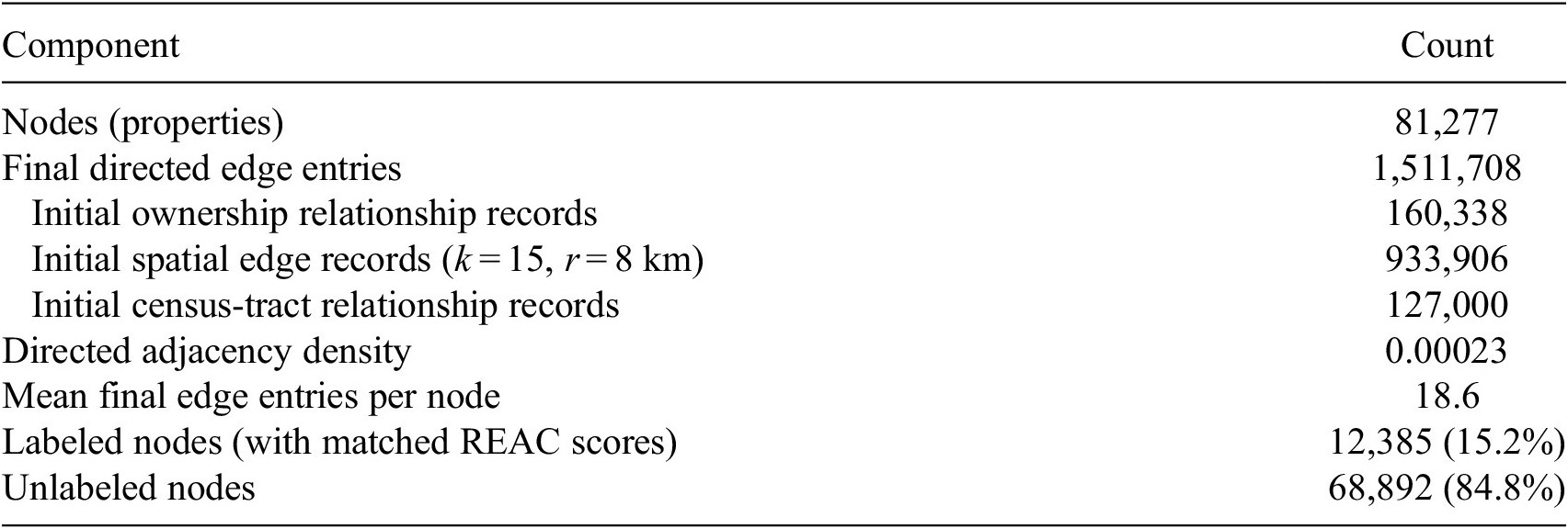


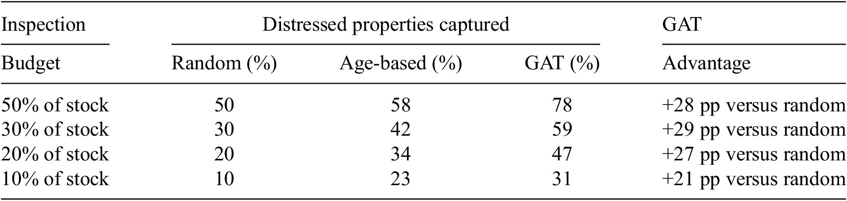

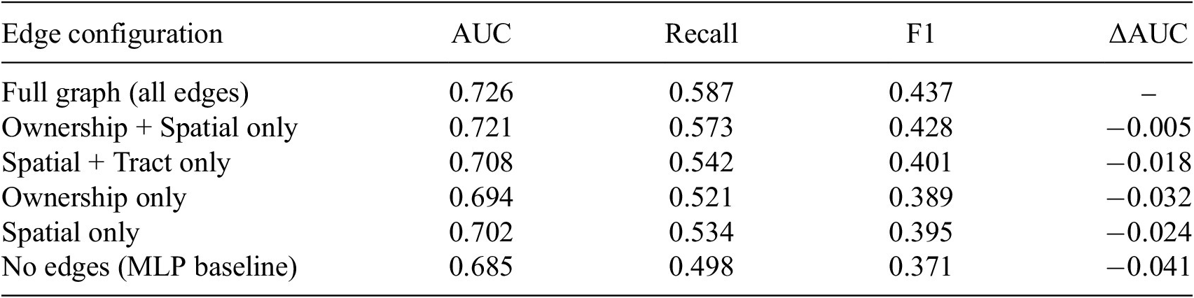


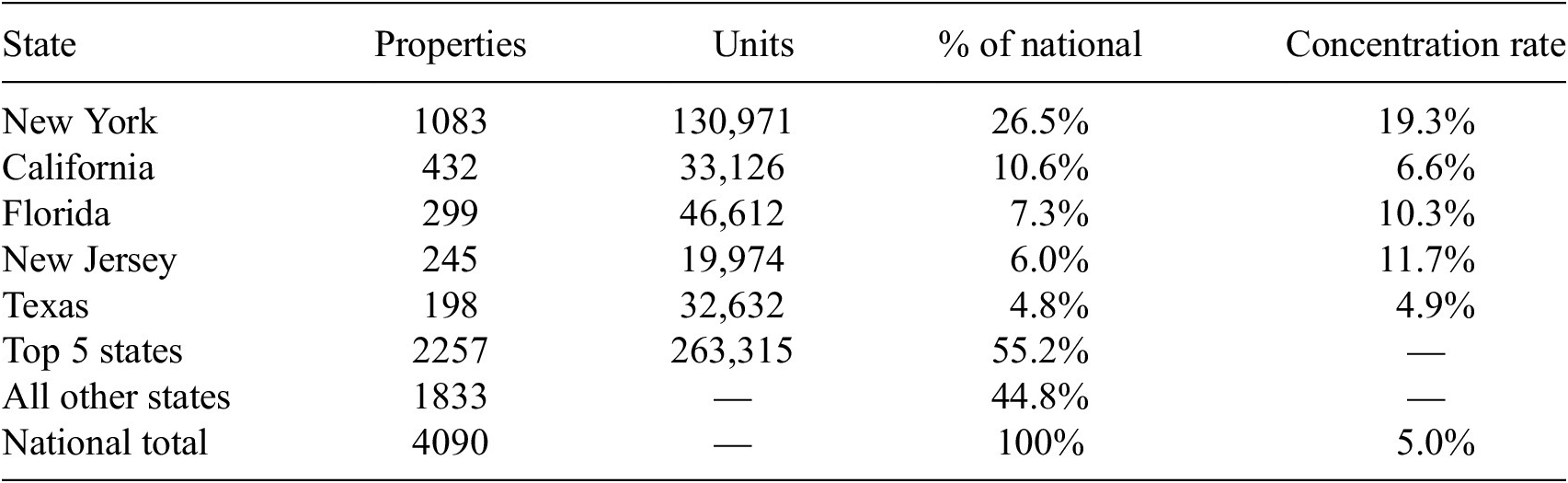

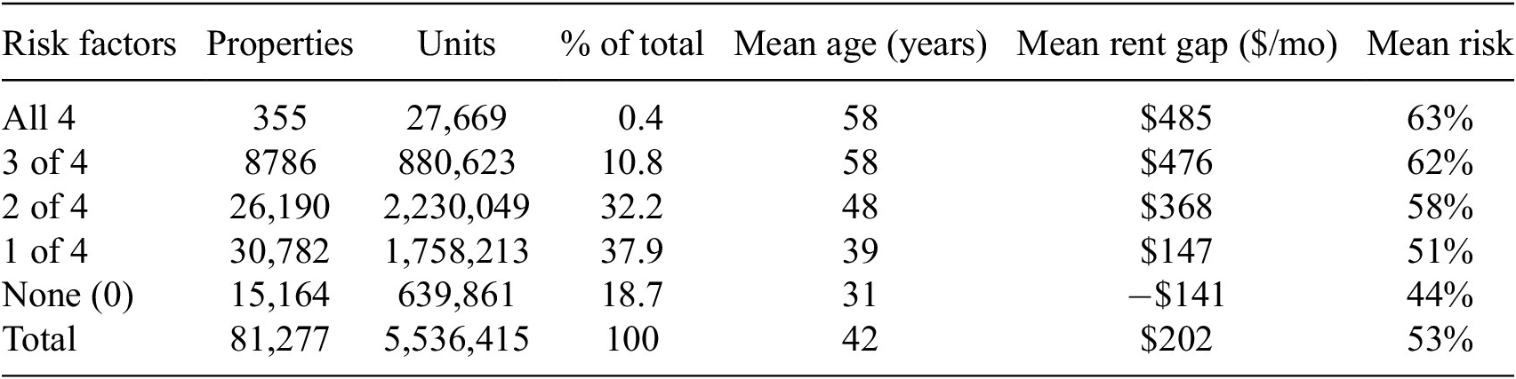
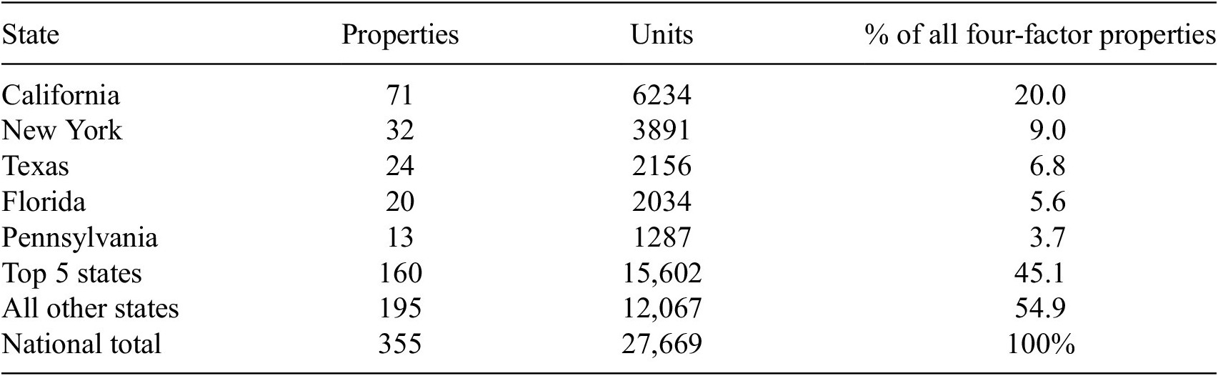
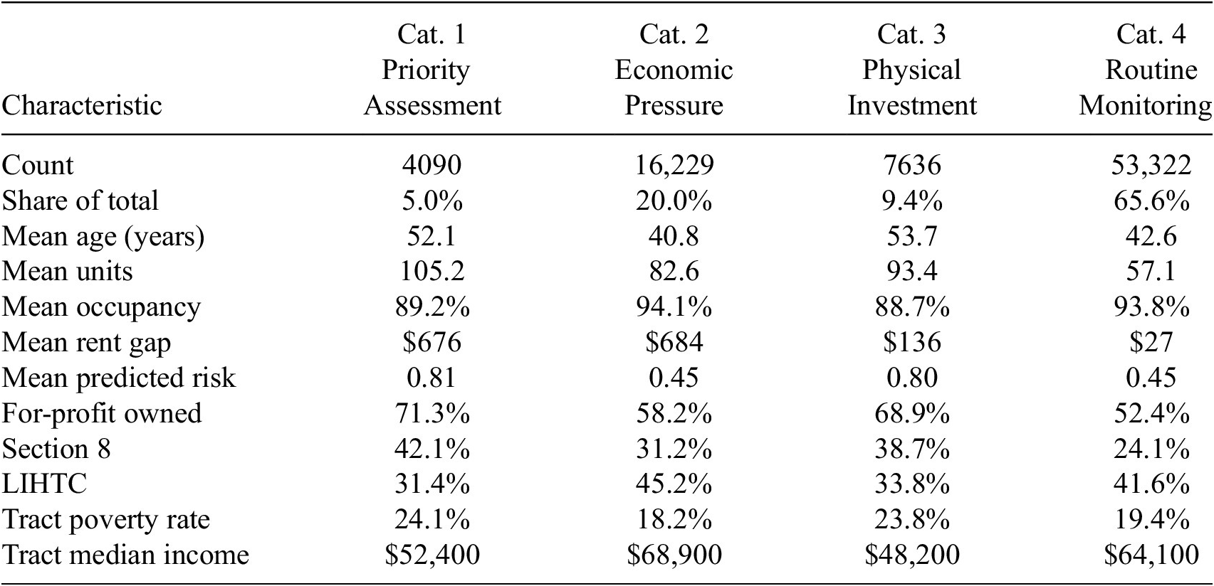


 Open access


Comments
No Comments have been published for this article.