1. Introduction
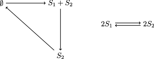
Reaction network models are often used to study the dynamics of the abundances of species from various branches of chemistry and biology. Here, the word ‘species’ can refer to different (bio)chemical molecules or different animal species, depending on the context. These networks take the form of directed graphs in which the vertices, often termed complexes in the domains of interest, are linear combinations of the species over the non-negative integers and the directed edges, which imply a state transition for the associated dynamical system, are termed reactions. See Figure 1 for an example of a reaction network.
A reaction network with two species:
 $S_1$
and
 $S_2$
. The vertices are linear combinations of the species over the integers. The directed edges are termed reactions and determine the net change in the counts of the species due to one instance of the reaction. For example, the reaction
 $S_1 + S_2 \to S_2$
reduces the count of
 $S_1$
by one, but does not affect the count of
 $S_2$
.

To each such graph a quantity termed the deficiency can be computed, and this quantity has been central to many classical results pertaining to the associated dynamical systems [Reference Anderson and Cotter4, Reference Anderson, Craciun and Kurtz5, Reference Anderson and Nguyen6, Reference Cappelletti and Wiuf9, Reference Feinberg11, Reference Horn13, Reference Horn and Jackson15]. To compute the deficiency, we first note that the vertices of a reaction network, which will be denoted by y and/or y
 $^{\prime}$
throughout this paper, can be viewed as vectors in
 ${\mathbb{Z}}^n_{\ge0}$
. For example, the vertices in Figure 1 can be associated with the vectors
 $\left[\begin{smallmatrix}0\\ 0\end{smallmatrix}\right]$
,
 $\left[\begin{smallmatrix}1\\1\end{smallmatrix}\right]$
,
 $\left[\begin{smallmatrix}0\\1\end{smallmatrix}\right]$
,
 $\left[\begin{smallmatrix}2\\0\end{smallmatrix}\right]$
, and
 $\left[\begin{smallmatrix}0\\2\end{smallmatrix}\right]$
. Moreover, a directed edge between two such vectors,
 $y \to y'$
, implies a state update of the form
 $y'-y \in {\mathbb{Z}}^n$
. The set of state update vectors implied by the graph is called the set of reaction vectors for the model. Viewing things in this manner, the deficiency for the graph provides a relation between the number of vertices, the number of connected components, and the dimension of the space spanned by the reaction vectors. The formal definition of deficiency is given in Definition 2.6.
Given the importance of the deficiency-zero property, it is natural to ask how common this property is. There are a number of ways one can tackle this question, including a simple enumeration of all networks of a given size. In fact, the earliest attempt to answer this question can be traced back to work by Horn in 1973 [Reference Horn14]. In that paper, Horn considered all reaction networks with exactly three vertices, each of which satisfies
 $\sum_{i = 1}^n y_i \le 2$
, where
 $y_i$
denotes the ith component of the vector associated with a vertex y, but with no condition on the number of species. Horn found 43 isomorphism classes of such networks, and among these, 41 have deficiency zero.
We choose a different approach by considering networks with a fixed number of species, say n, and then quantifying the prevalence of the deficiency-zero property via limit theorems (as
 $n\to \infty$
) in an Erdös–Rényi random graph framework in which there is an equal probability,
 $p_n$
, that there is an edge between any two vertices. However, we are immediately confronted with a modeling problem: for any finite number of species there are an infinite number of possible graphs that can be constructed from them. For example, with just the single species
 $S_1$
, possible vertices include
 $S_1$
,
 $2S_1$
,
 $3S_1$
, … Hence, we must restrict ourselves in some manner so that for a given number of species, only a finite number of vertices are possible.
In this paper we restrict ourselves to studying so-called ‘binary’ reaction networks, whose vertices satisfy
 $\sum_{i = 1}^n y_i \le 2$
. Such models are quite common in the literature. Our main finding is that in such a scenario
 $r(n)=\frac{1}{n^3}$
is a threshold function in that if
 $p_n \ll r(n)$
as
 $n\to \infty$
, then the probability of deficiency zero converges to 1, whereas if
 $p_n \gg r(n)$
, then the probability of deficiency zero converges to 0; see Theorems 4.1 and 4.2. Moreover, along the way we prove that in the setting of
 $p_n\ll r(n)$
, with high probability all the connected components of deficiency-zero reaction networks will consist of pairs of vertices. Intriguingly, paired reaction networks can be found in certain models of autocatalytic cycles related to the study of the origin of life [Reference Peng, Plum, Gagrani and Baum16].
The remainder of this paper is organized as follows. In Section 2 we briefly review some key terminology of reaction network theory, and provide some preliminary results related to deficiency. In Section 3, we set up the Erdös–Rényi random graph framework for reaction networks. In Section 4 we present our main results, which quantify the prevalence of deficiency-zero reaction networks in our chosen framework. Finally, in Section 5 we end with a brief discussion.
2. Chemical reaction networks
Here we formally introduce reaction networks and deficiency. Moreover, we collect some preliminary results related to the deficiency of a reaction network.
2.1 Reaction networks and key definitions
Let
 $\{S_1,\dots,S_n\}$
be a set of n species undergoing a finite number of reaction types. We denote a particular reaction by
 $y \to y'$
, where y and y
 $^{\prime}$
are linear combinations of the species on
 $\{0,1,2,\dots\}$
representing the number of molecules of each species consumed and created in one instance of that reaction, respectively. The linear combinations y and y
 $^{\prime}$
are often called complexes of the system. For a given reaction,
 $y\to y'$
, y is called the source complex and y
 $^{\prime}$
is called the product complex. A complex can be both a source complex and a product complex. However, a complex cannot be both the source and product for a single reaction, nor do we include isolated complexes that are not involved in any reaction. We may associate each complex with a vector in
 $\mathbb{Z}^n_{\geq 0}$
whose coordinates give the number of molecules of the corresponding species in the complex. As is common in the reaction network literature, both ways of representing complexes will be used interchangeably throughout the paper. For example, if the system has two species,
 $\{S_1,S_2\}$
, the reaction
 $S_1+S_2\to 2S_2$
has
 $y=S_1+S_2$
, which is associated with the vector
 $\left[\begin{smallmatrix}1\\1\end{smallmatrix}\right]$
, and
 $y'=2S_2$
, which is associated with the vector
 $\left[\begin{smallmatrix}0\\2\end{smallmatrix}\right]$
. Viewing the complexes as vectors, the reaction vector associated to the reaction
 $y\to y'$
is simply
 $y'-y\in {\mathbb{Z}}^n$
, which gives the state update of the system due to one occurrence of the reaction.
Definition 2.1. For
 $n \ge 0$
, let
 $\mathcal{S} =\{S_1, \ldots, S_n\}$
,
 $\mathcal{C}=\cup_{y\to y'}\{y,y'\}$
, and
 $\mathcal{R}=\cup_{y\to y'}\{y\to y'\}$
be the sets of species, complexes, and reactions, respectively. The triple
 $\{\mathcal{S,C,R}\}$
is called a reaction network. When
 $n = 0$
, in which case
 $\mathcal{S} = \mathcal{C} = \mathcal{R} = \emptyset$
, the network is termed the empty network.
For each reaction network
 $\{\mathcal{S,C,R}\}$
there is a unique directed graph constructed in the obvious manner: the vertices of the graph are given by
 $\mathcal{C}$
and a directed edge is placed from y to y
 $^{\prime}$
if and only if
 $y \to y' \in \mathcal{R}$
. Figure 1 is an example of such a graph. Note that by definition the directed graph associated to a reaction network contains only vertices corresponding to elements in
 $\mathcal{C}$
involved in some reaction, i.e. the degree of all vertices is at least 1 and so isolated vertices are not present in the associated network. We denote by
 $\ell$
the number of connected components of the graph.
Remark 2.1. Note that since each connected component must consist of at least two vertices, we have the bound
 $\ell \le \frac{|\mathcal{C}|}{2}$
.
Definition 2.2. The linear subspace generated by all reaction vectors is called the stoichiometric subspace of the network. Denote by
 $s=\dim(\mathrm{span}\{y'-y\,{:}\,y\to y'\in\mathcal{R}\})$
the dimension of the stoichiometric subspace. Note that
 $s \le n$
, where n is the number of species. This fact will be used a number of times in this paper.
Definition 2.3. A vertex,
 $y \in {\mathbb{Z}}^n_{\ge 0}$
, is called binary if
 $\sum_{i = 1}^n y_i = 2$
. A vertex is called unary if
 $\sum_{i = 1}^n y_i = 1$
. The vertex
 $\vec{0} \in {\mathbb{Z}}^n$
is said to be of zeroth order.
Definition 2.4. A reaction network
 $\{\mathcal{S,C,R}\}$
is called binary if each vertex is binary, unary, or of zeroth order.
As discussed in the introduction, we will focus on binary reaction networks in this paper. The following type of network will play a key role.
Definition 2.5. A reaction network is called paired if each of its connected components contains precisely two vertices. A reaction network is called i-paired if it is paired and contains i connected components.
2.2 Deficiency of a reaction network
Definition 2.6. The deficiency of a reaction network
 $\{\mathcal{S,C,R}\}$
is
 $\delta=|\mathcal{C}|-\ell-s$
, where
 $|\mathcal{C}|$
is the number of vertices,
 $\ell$
is the number of connected components of the associated graph, and
 $s = \dim(\text{span}\{y'-y\,{:}\, y\to y'\in \mathcal{R}\})$
is the dimension of the stoichiometric subspace of the network.
For each
 $j\le \ell$
, we let
 $\mathcal{C}_j$
denote the collection of vertices in the jth connected component,
 $s_j$
be the corresponding dimension of the span of the reaction vectors of that component, and we define
 $\delta_j = |\mathcal{C}_j| - 1 - s_j$
to be the deficiency of that component.
We collect a number of basic properties of deficiency in the following lemma.
Lemma 2.1. Let
 $n \ge 1$
and let
 $\{\mathcal{S},\mathcal{C},\mathcal{R}\}$
be a reaction network with n species.
-
(a)
 $\delta$
does not depend upon the direction of the edges.
-
(b)
$s_j \le |\mathcal{C}_j| - 1$
, and so
$\delta_j \ge 0$
. -
(c)
$s \le |\mathcal{C}| - \ell$
, and so
$\delta \ge 0$
. -
(d)
$\delta = 0$
if and only if both the following conditions hold:-
i.
$s_j = |\mathcal{C}_j| - 1$
for each
$j\le \ell$
(equivalently,
$\delta_j= 0$
for each
$j\le \ell$
). -
ii.
$\sum_{j=1}^\ell s_j = s$
.
-
-
(e) If
$\delta = 0$
, then
$|\mathcal{C}| \le 2n$
. -
(f) Suppose the reaction network is paired, and that
$\zeta_j$
is a reaction vector from the jth connected component. Then
$\delta=0$
if and only if
$\cup_{j=1}^\ell\{\zeta_j\} = \{\zeta_1,\dots,\zeta_\ell\}$
are linearly independent. -
(g) (Monotonicity of deficiency.) Let
$\{\widehat{\mathcal{S}},\widehat{\mathcal{C}},\widehat{\mathcal{R}}\}$
and
$\{\mathcal{S},\mathcal{C},\mathcal{R}\}$
be two reaction networks with
$\widehat{\mathcal{R}}\setminus \mathcal{R} = \{y\to y'\}$
, a single reaction. Let
$\hat \delta$
and
$\delta$
be the deficiencies of the two networks. Then
$\hat\delta \geq \delta$
.








Proof.
-
(a) This follows from the definition of deficiency.
-
(b) This follows from the observation that a cycle within a connected component implies a dependency among the reaction vectors.
-
(c) This follows from (b) since
$\mathcal{C} = \cup_{j=1}^\ell \mathcal{C}_j$
and
$s \le \sum_{j=1}^\ell s_j$
. -
(d) This follows in a straightforward manner from (b) and (c).
-
(e) From the definition of deficiency
$\delta = |\mathcal{C}|-\ell-s$
, the fact that
$s\leq n$
, and
$\ell\leq \frac{|\mathcal{C}|}{2}$
(from Remark 2.1), we have
$\delta \geq |\mathcal{C}|- \frac{|\mathcal{C}|}{2} -n =\frac{|\mathcal{C}|}{2}-n$
. Since the reaction network has deficiency zero, we therefore have
$0\geq \frac{|\mathcal{C}|}{2} -n$
, which implies
$|\mathcal{C}|\le 2n$
. -
(f) Since the reaction network is paired, we have
$s_j=1$
and
$|\mathcal{C}_j|=2$
for each
$j\leq \ell$
. Thus, condition (i) in (d) is satisfied. Since
$s_j=1$
, condition (ii) in (d) holds if and only if all
$\zeta_j$
are linearly independent. -
(g) Let
$\ell,s$
and
$\hat{\ell},\hat{s}$
be the number of connected components and dimension of the stoichiometric subspace of
$\{\mathcal{S},\mathcal{C},\mathcal{R}\}$
and
$\{\widehat{\mathcal{S}},\widehat{\mathcal{C}},\widehat{\mathcal{R}}\}$
, respectively.Case 1:
$y,y'\in\mathcal{C}$
, and y and y
$^{\prime}$
are from the same connected component. In this case, we have
$|\widehat{\mathcal{C}}|=|\mathcal{C}|$
and
$\hat{\ell}=\ell$
. Since y and y
$^{\prime}$
are from the same connected component, the reaction vector
$y'-y$
can be written as the linear combination of the remaining reaction vectors from its connected component. Therefore, adding
$y\to y'$
to
$\{\mathcal{S},\mathcal{C},\mathcal{R}\}$
does not increase the dimension of its stoichiometric subspace. Thus,
$\hat{s}=s$
and
$\hat\delta=\delta$
.Case 2:
$y,y'\in\mathcal{C}$
, and y and y
$^{\prime}$
are from different connected components. In this case, we have
$|\widehat{\mathcal{C}}|=|\mathcal{C}|$
and
$\hat{\ell}=\ell-1$
. Since we are adding one reaction to
$\{\mathcal{S},\mathcal{C},\mathcal{R}\}$
to obtain
$\{\widehat{\mathcal{S}},\widehat{\mathcal{C}},\widehat{\mathcal{R}}\}$
, we add at most one dimension to the stoichiometric subspace of
$\{\mathcal{S},\mathcal{C},\mathcal{R}\}$
. Thus,
$\hat{s}\leq s+1$
and
$\hat\delta=|\widehat{\mathcal{C}}|-\hat{\ell}-\hat{s} \geq |\mathcal{C}| - (\ell-1) - (s+1) = \delta$
.Case 3:
$y \in \mathcal{C}$
and
$y' \notin \mathcal{C}$
, or vice versa. In this case, we have
$|\widehat{\mathcal{C}}|=|\mathcal{C}|+1$
and
$\hat{\ell}=\ell$
. Similar to the previous case, we must have
$\hat{s}\leq s+1$
, and thus
$\hat\delta=|\widehat{\mathcal{C}}|-\hat{\ell}-\hat{s} \geq |\mathcal{C}|+1 - \ell - (s+1) = \delta$
.Case 4:
$y,y'\notin \mathcal{C}$
. In this case we have
$|\widehat{\mathcal{C}}|=|\mathcal{C}|+2$
and
$\hat{\ell}=\ell+1$
. Similar to the previous cases, we still have
$\hat{s}\leq s+1$
and thus
$\hat\delta=|\widehat{\mathcal{C}}|-\hat{\ell}-\hat{s} \geq |\mathcal{C}|+2- (\ell+1) - (s+1) = \delta$
.















Remark 2.2. Lemma 2.1(g) implies that if we remove a reaction from a reaction network with deficiency zero, then the resulting network also has deficiency zero. This means that deficiency zero is a monotone decreasing property, which guarantees that a threshold function for deficiency zero exists (see [Reference Bollobás and Thomason8]).
We illustrate the concept of deficiency via two examples.
Example 2.1. (Enzyme kinetics [Reference Anderson, Craciun and Kurtz5]) Consider a reaction network with species
 $\{S$
, E, SE,
 $P\}$
and associated graph
 $S+E \leftrightarrows SE \leftrightarrows P+E$
,
 $E \leftrightarrows \emptyset \leftrightarrows S$
. In this example, the reaction network has
 $|\mathcal{C}|=6$
vertices, there are
 $\ell=2$
connected components, and the dimension of the stochiometric subspace is
 $s=4$
. Thus, the deficiency is
 $\delta = 6-2-4=0$
.
The following example demonstrates that it is sometimes most natural to use Lemma 2.1(f) to verify that a network has a deficiency of zero.
Example 2.2. (Binary, 3-paired network) Consider a reaction network with species
 $\{S_1, S_2, \dots, S_9\}$
and associated graph
 $S_1 + S_2 \rightleftarrows S_3 + S_4$
,
 $S_1 + S_3 \rightleftarrows S_5 + S_6$
,
 $S_6+S_7 \rightleftarrows S_8+S_9$
. This network is paired in the sense of Definition 2.5. Moreover, there is linear independence among the connected components, which can be seen easily since each connected component has a species not found in any other connected component. Hence, Lemma 2.1(f) implies that the deficiency of this network is zero.
3. Erdös–Rényi model for binary reaction networks
As alluded to in the introduction, the vast majority of reaction network models found in the literature are binary. Hence, those are the focus of the current paper.
Let the set of species be
 $\mathcal{S}=\{S_1,S_2,\dots,S_n\}$
. We consider binary reaction networks with species in
 $\mathcal{S}$
. The set of all possible vertices is then
 $\mathcal{C}^0_n = \{\emptyset, S_i, S_i+S_j$
for
 $1 \le i \le n$
and
 $1 \le j \le n\}$
. For a given n, we denote by
 $N_n = |\mathcal{C}^0_n|$
the cardinality of
 $\mathcal{C}^0_n$
. Thus,
 $N_n$
is the total number of possible zeroth-order, unary, and binary vertices that can be generated from n distinct species. A straightforward calculation gives
 $N_n=1+n+n+\frac{1}{2}n(n-1) = \frac{1}{2}(n^2+3n+2)$
, and so
 $n \sim \sqrt{2N_n}$
. Here, we use the notation
 $\sim$
in the standard way: for any two sequences of real numbers
 $\{a_n\}$
and
 $\{b_n\}$
, we write
 $a_n\sim b_n$
if
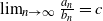 $\lim_{n\to \infty} \frac{a_n}{b_n} = c$
for some constant
 $c \in {\mathbb{R}}$
.
We consider an Erdös–Rényi random graph
 $G(N_n,p_n)$
, which we will simply denote by
 $G_n$
throughout, where the set of vertices is the set
 $\mathcal{C}^0_n$
, and the probability that there is an edge between any two particular vertices is
 $p_n$
, independently of all other edges. To each such random graph a reaction network graph can be associated in the following way:
-
• each vertex with positive degree in the random graph represents a vertex in the reaction network, and
-
• each edge in the random graph represents a reaction in the reaction network (we can assume all reactions are reversible, i.e. that
$y\to y'\in \mathcal{R} \implies y'\to y \in \mathcal{R}$
, since we do not need to worry about direction—see Lemma 2.1(a)).

We will denote the reaction network associated with the graph
 $G(N_n,p_n)$
by
 $R_n$
. We will denote the deficiency of
 $R_n$
by
 $\delta_{R_n}$
.
In order to solidify the notation, we present below the cases
 $n=1$
and
 $n=2$
.
Example 3.1. (The case with
 $n=1$
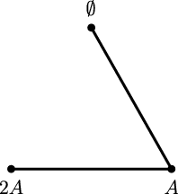
species) Denote the only species by A. The set of vertices, or equivalently the set of all possible complexes, is
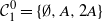 $\mathcal{C}^0_1=\{\emptyset ,A,2A\}$
. Figure 2 shows one possible realization of the random graph
 $G(N_1,p)$
when
 $p \in (0,1)$
. The associated reaction network
 $R_1$
for the particular graph shown in Figure 2 is
 $\emptyset \leftrightarrows A \leftrightarrows 2A$
.
A realization of a random graph when
 $n=1$
and
 $p\in (0,1)$
. The associated reaction network is
 $\emptyset \leftrightarrows A \leftrightarrows 2A$
.

Example 3.2 (The case with
 $n=2$
species) Denote the set of species by
 $\mathcal{S}=\{A,B\}$
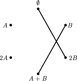
. The set of vertices is
 $\mathcal{C}^0_2=\{\emptyset,A,B,2A,2B,A+B\}$
. Figure 3 illustrates a possible realization of the random graph
 $G(N_2,p)$
when
 $p \in (0,1)$
. The associated reaction network
 $R_2$
for the particular graph shown in Figure 2 is
 $\emptyset \leftrightarrows 2B$
,
 $B \leftrightarrows A+B$
.
A realization of a random graph when
 $n=2$
and
 $p\in (0,1)$
.

4. The threshold function for deficiency zero
The goal of this section is to prove that
 $r(n) = \frac1{n^3}$
is a threshold function in that
 \begin{equation*} \lim_{n\to\infty}\mathbb{P}(\delta_{R_n} = 0) = \begin{cases} 0 &\text{if } p_n \gg r(n) , \\ \\[-8pt] 1 & \text{if } p_n \ll r(n). \end{cases}\end{equation*}
Throughout this section we will make use of the standard notation
 $a_n \ll b_n$
or
 $b_n \gg a_n$
to mean
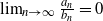 $\lim_{n\to \infty} \frac{a_n}{b_n} = 0$
whenever
 $\{a_n\}$
and
 $\{b_n\}$
are sequences of non-negative real numbers. We also remind the reader that we write
 $a_n \sim b_n$
to mean
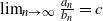 $\lim_{n\to \infty} \frac{a_n}{b_n} = c$
for some constant
 $c \in {\mathbb{R}}_{>0}$
.
4.1. The case
$p_n\gg r(n)$

This case is relatively straightforward. We will show that if
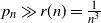 $p_n \gg r(n)=\frac{1}{n^3}$
, then with high probability we have
 $|\mathcal{C}|>2n$
. In this case, Lemma 2.1(e) implies that the associated reaction network does not have deficiency zero.
Since
 $|\mathcal{C}|$
is the number of non-isolated vertices in
 $G_n$
, we start with a lemma regarding the number of isolated vertices in
 $G_n$
.
Lemma 4.1. Suppose
 $p_n = \frac{2n+\alpha_n}{N_n(N_n-1)}$
, with
 $\alpha_n \gg n^{1/2}$
. Let I be the set of isolated vertices in
 $G_n$
, that is
 $I =\big\{ v\in \mathcal{C}^0_n \,{:}\, \mathrm{deg}(v)=0\big\}$
. Then we have
 $\lim_{n\to\infty}\mathbb{P}(|I|\geq N_n-2n)=0$
.
Proof. We require both
 $\mathbb{E} ( |I|)$
and
 $\text{Var} (|I|)$
. First, a straightforward calculation yields
 \begin{align*} \mathbb{E} (|I|) &= \mathbb{E} \left[\sum_{v\in \mathcal{C}^0_n} \textbf{1}_{\{\deg(v)=0\}}\right] =N_n\mathbb{P}(\deg(v)=0)=N_n(1-p_n)^{N_n-1}.\end{align*}
Turning to the variance, we have
 \begin{align*} \left| I \right|^2 = \sum_{v,w \in \mathcal{C}^0_n}\textbf{1}_{\{\deg(v)=\deg(w)=0\}} = \sum_{v\in \mathcal{C}^0_n}\textbf{1}_{\{\deg(v)=0\}}+ \sum_{v,w \in \mathcal{C}^0_n: v\neq w}\textbf{1}_{\{\deg(v)=\deg(w)=0\}}.\end{align*}
Therefore, we have
 \begin{align*} \text{Var} (|I|) &= \mathbb{E}(|I|^2) - \mathbb{E}(|I|)^2 \\ &= \mathbb{E}\Bigg[\sum_{v\in \mathcal{C}^0_n}\textbf{1}_{\{\deg(v)=0\}}+ \sum_{v,w \in \mathcal{C}^0_n: v\neq w}\textbf{1}_{\{\deg(v)=\deg(w)=0\}}\Bigg]- N_n^2(1-p_n)^{2N_n-2} &=N_n(1-p_n)^{N_n-1} +N_n(N_n-1)(1-p_n)^{2N_n-3} - N_n^2(1-p_n)^{2N_n-2} \\[3pt] &=N_n(1-p_n)^{N_n-1}(1-(1-p_n)^{N_n-2})+N_n^2(1-p_n)^{2N_n-3}p_n \\[3pt] &\leq N_n(1-p_n)^{N_n-1}(N_n-2)p_n + N_n^2(1-p_n)^{2N_n-3}p_n \\[3pt] &\leq N_n(N_n-2)p_n+N_n^2p_n \leq 2N_n^2p_n,\end{align*}
where the first inequality follows from Bernoulli’s inequality.
We will utilize
 $\mathbb{E}(|I|)$
and
 $\text{Var}(|I|)$
to show that
 $\lim_{n\to\infty}\mathbb{P}(|I|\geq N_n-2n) = 0$
. It suffices to prove this in the three cases below.
When
 $\alpha_n \sim N_n$
we have
 $p_n\sim \frac{1}{N_n}$
, and thus
 $p_n > \frac{c}{N_n}$
for some constant
 $c>0$
and n large enough. Therefore,
 $\mathbb{E}(|I|) = N_n(1-p_n)^{N_n-1} \le N_n\Big(1-\frac{c}{N_n}\Big)^{N_n-1}\le N_n \mathrm{e}^{-c}$
. Applying Chebyshev’s inequality yields
 \begin{equation*} \mathbb{P}(|I|>N_n-2n) \leq \frac{\text{Var}(|I|)}{(N_n-2n-E[|I|])^2}\le\frac{2N_n^2p_n}{(N_n-2n-N_n\mathrm{e}^{-c})^2} = \frac{2p_n}{(1-2n/N_n-\mathrm{e}^{-c})^2}.\end{equation*}
Since
 $p_n\sim\frac{1}{N_n}$
and
 $N_n \sim n^2$
, we have
 $\lim_{n\to\infty}\mathbb{P}(|I|>N_n-2n)=0$
.
The next case is when
 $\alpha_n\ll N_n$
, or equivalently when
 $p_n\ll\frac{1}{N_n}$
. Using Taylor’s expansion, we have
 $\mathbb{E}(|I|)=N_n(1-p_n)^{N_n-1} \leq N_n\big(1-p_n(N_n-1)+\frac{1}{2}p_n^2(N_n-1)(N_n-2)\big)$
. Again, we apply Chebyshev’s inequality:
 \begin{align*} \mathbb{P}(|I|\geq N_n-2n) & \leq \frac{\text{Var}(|I|)}{(N_n-2n-E[|I|])^2} \\ & \leq \frac{2N_n^2p_n}{\big(N_n-2n-N_n+N_n(N_n-1)p_n-\frac{1}{2}N_n(N_n-1)(N_n-2)p_n^2\big)^2} \\ & = \frac{2N_n^2p_n}{\big({-}2n+N_n(N_n-1)p_n-\frac{1}{2}N_n(N_n-1)(N_n-2)p_n^2\big)^2}. \end{align*}
Now we plug in
 $p_n=\frac{2n+\alpha_n}{N_n(N_n-1)}$
:
 \begin{align*} \mathbb{P}(|I|\geq N_n-2n) & \leq \frac{\frac{2N_n}{N_n-1}(2n+\alpha_n)}{\Big(\!-2n+2n+\alpha_n-\frac{N_n-2}{2N_n(N_n-1)}(2n+\alpha_n)^2\Big)^2} \\ & = \frac{2N_n}{N_n-1}\frac{2n+\alpha_n}{\Big(\alpha_n-\frac{N_n-2}{2N_n(N_n-1)}(2n+\alpha_n)^2\Big)^2}.\end{align*}
If
 $\alpha_n\ll n$
or
 $\alpha_n\sim n$
, we have
 \begin{equation*} \frac{2n+\alpha_n}{\Big(\alpha_n-\frac{N_n-2}{2N_n(N_n-1)}(2n+\alpha_n)^2\Big)^2} \sim \frac{n}{\alpha_n^2} \to 0 \end{equation*}
as
 $n\to\infty$
, since
 $\alpha_n \gg n^{1/2}$
. If
 $\alpha_n\gg n$
, we have
 \begin{equation*} \frac{2n+\alpha_n}{\Big(\alpha_n-\frac{N_n-2}{2N_n(N_n-1)}(2n+\alpha_n)^2\Big)^2} \sim \frac{\alpha_n}{\alpha_n^2} = \frac{1}{\alpha_n} \to 0 \end{equation*}
as
 $n\to\infty$
, since
 $\alpha_n\ll N_n$
. Thus, either way we must have
 $\lim_{n\to\infty}\mathbb{P}(|I|>N_n-2n)=0$
.
When
 $\alpha_n \gg N_n$
, we can apply the same argument as in the second case, since
 \begin{equation*} \frac{2n+\alpha_n}{\Big(\alpha_n-\frac{N_n-2}{2N_n(N_n-1)}(2n+\alpha_n)^2\Big)^2} \ll \frac{\alpha_n}{\alpha_n^2} = \frac{1}{\alpha_n} \to 0.\end{equation*}
In all three cases we have
 $\lim_{n\to\infty}\mathbb{P}(|I|\geq N_n-2n)=0$
.
We are now ready to provide the first main theorem.
Theorem 4.1. Let
 $G_n$
denote the Erdös–Rényi random graph with
 $N_n$
vertices and edge probability
 $p_n$
, and let
 $R_n$
be the reaction network associated to
 $G_n$
. When
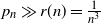 $p_n \gg r(n)=\frac1{n^3}$
, we have
 $\lim_{n\to\infty} \mathbb{P}(\delta_{R_n}=0)=0$
.
Proof. Note that the vertices of the reaction network
 $R_n$
correspond to the vertices in
 $G_n$
with positive degree. Thus, letting I denote the set of isolated vertices of
 $G_n$
, Lemma 2.1(e) implies that if the network is deficiency zero, we must have
 $|I| \geq N_n-2n $
. From this, we have
 $\mathbb{P}(\delta_{R_n} =0)\leq \mathbb{P}(|I|\geq N_n-2n)$
. Since
 $ r(n)=\frac{1}{n^3}\sim \frac{n}{N_n^2}$
and
 $p_n\gg r(n)$
, we have that
 $p_n$
satisfies the condition in Lemma 4.1. Hence, using Lemma 4.1, we have
 $\lim_{n\to\infty} \mathbb{P}(\delta_{R_n}=0)=\lim_{n\to \infty} \mathbb{P}(|I| \ge N_n - 2n) = 0$
.
4.2. The case
$p_n\ll r(n)$

We will show that in the case
 $p_n\ll r(n)$
it is enough to focus on paired reaction networks, which are introduced in Section 2. We first state the main theorem.
Theorem 4.2. Let
 $G_n$
denote the Erdös–Rényi random graph with
 $N_n$
vertices and edge probability
 $p_n$
, and let
 $R_n$
be the reaction network associated to
 $G_n$
. When
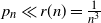 $p_n \ll r(n)=\frac1{n^3}$
, we have
 $\lim_{n\to\infty}\mathbb{P}(\delta_{R_n} =0)=1$
.
Proof. We have
 $\mathbb{P}(\delta_{R_n}=0) = \mathbb{P}(\delta_{R_n}=0, R_n$
is paired
 $) + \mathbb{P}(\delta_{R_n}=0, R_n$
is not paired
 $) \geq \mathbb{P}(\delta_{R_n}=0, R_n$
is paired). Therefore, it suffices to show that
 $\lim_{n\to\infty}\mathbb{P}(\delta_{R_n}=0, R_n$
is paired
 $)\,{=}\, 1$
. Noting that, for deficiency-zero models, the number of reversible reaction vectors is bounded above by n, we have
 \begin{align} \mathbb{P}(\delta_{R_n} & = 0, R_n \text{ is paired} ) \nonumber \\[3pt] & = \sum_{i=1}^n\mathbb{P}(\delta_{R_n}=0, R_n \text{ is \textit{i}-paired} ) \nonumber \\[3pt] & = \sum_{i=1}^n\mathbb{P}(\delta_{R_n}=0 \mid R_n \text{ is \textit{i}-paired} )\mathbb{P}(R_n \text{ is \textit{i}-paired}) \nonumber \\[3pt] & = \sum_{i=1}^n \mathbb{P}(\delta_{R_n}=0 \mid R_n \text{ is \textit{i}-paired} )\frac{N_n!}{i!2^i(N_n-2i)!}p_n^i (1-p_n)^{N_n(N_n-1)/2-i} \nonumber \\[3pt] & \geq \sum_{i=1}^n \mathbb{P}(\delta_{R_n}=0 \mid R_n \text{ is \textit{i}-paired} )\frac{(N_n-2i)^{2i}}{i!2^i}p_n^i (1-p_n)^{N_n(N_n-1)/2-i} ;\end{align}
the third equality uses that the number of i-paired graphs is
 $\left(\begin{smallmatrix}N_n\\ 2 \end{smallmatrix}\right)\left(\begin{smallmatrix}N_n-2\\ 2 \end{smallmatrix}\right)\cdots \left(\begin{smallmatrix}N_n-2i+2\\ 2 \end{smallmatrix}\right)$
, with the repetition of the graphs accounted for by division by
 $i!$
.
Note that because
 $p_n \ll 1/n^3$
and
 $N_n \sim n^2$
, we have
 $N_n^2p_n \ll n$
. Now let
 $k_n$
satisfy
 $\lim_{n\to\infty}k_n=\infty$
and
 $N_n^2 p_n \ll k_n\ll n$
. Cutting off the last
 $n-k_n$
terms from (4.1) yields
 \begin{align} \mathbb{P}(\delta_{R_n} & = 0, R_n \text{ is paired} ) \nonumber \\[3pt] & \ge \sum_{i=1}^{k_n} \mathbb{P}(\delta_{R_n}=0 \mid R_n \text{ is \textit{i}-paired} )\frac{(N_n-2i)^{2i}}{i!2^i}p_n^i (1-p_n)^{N_n(N_n-1)/2-i} \nonumber \\[3pt] & \geq \sum_{i=1}^{k_n}\bigg(1-c\frac{i^4}{n^4}\bigg)\bigg(1-\frac{21i}{n}\bigg) \frac{(N_n-2i)^{2i}}{i!2^i}p_n^i (1-p_n)^{N_n(N_n-1)/2-i} \\[3pt] & \geq \bigg(1-c\frac{k_n^4}{n^4}\bigg)\bigg(1-\frac{21k_n}{n}\bigg)(1-p_n)^{N_n^2/2} \sum_{i=1}^{k_n}\frac{(N_n-2i)^{2i}}{i!2^i}p_n^i \nonumber\\[3pt] & \geq \bigg(1-c\frac{k_n^4}{n^4}\bigg)\bigg(1-\frac{21k_n}{n}\bigg)(1-p_n)^{N_n^2/2} \sum_{i=1}^{k_n}\frac{(N_n-2k_n)^{2i}}{i!2^i}p_n^i , \nonumber \end{align}
where the inequality in (4.2) will be proven using Lemma 4.2, Proposition 4.1, and Lemma 4.3 after the proof of the main theorem. The inequalities after (4.2) follow by noting that
 $i \le k_n$
.
Let
 $\lambda_n = \frac{1}{2}(N_n-2k_n)^2p_n$
, and note that
 $\lambda_n\ll k_n$
since we chose
 $N_n^2p_n\ll k_n$
. Using Taylor’s remainder theorem and Stirling’s approximation, we have
 \begin{align*} \sum_{i=1}^{k_n}\frac{\lambda_n^i}{i!} & \geq \mathrm{e}^{\lambda_n} - \frac{e^{\lambda_n}\lambda_n^{k_n+1}}{(k_n+1)!} \\ & \geq \mathrm{e}^{\lambda_n}\bigg(1-\frac{\lambda_n^{k_n+1}}{\sqrt{2\pi}(k_n+1)^{k_n+1}\mathrm{e}^{-k_n+1}}\bigg) \\ & = \mathrm{e}^{\lambda_n}\bigg(1-\frac{1}{\sqrt{2\pi}\,}\bigg(\frac{\lambda_n \mathrm{e}}{k_n+1}\bigg)^{k_n+1}\bigg).\end{align*}
Thus, we have
 \begin{multline*} \mathbb{P}(\delta_{R_n}=0, R_n \text{ is paired} ) \\ \geq \bigg(1-c\frac{k_n^4}{n^4}\bigg)\bigg(1-\frac{21k_n}{n}\bigg)(1-p_n)^{N_n^2/2} \mathrm{e}^{\lambda_n}\bigg(1-\frac{1}{\sqrt{2\pi}\,}\bigg(\frac{\lambda_n \mathrm{e}}{k_n+1}\bigg)^{k_n+1}\bigg).\end{multline*}
Since
 $\lambda_n\ll k_n\ll n$
, the first, second, and last terms converge to 1. Hence, it suffices to show that
 $\lim_{n\to\infty}(1-p_n)^{N_n^2/2} \mathrm{e}^{\lambda_n} =1$
, or
 $\lim_{n\to\infty}\frac{1}{2}N_n^2\ln(1-p_n) + \lambda_n \,{=}\,0$
. Since
 $p_n\ll 1$
, we have
 $-p_n-p_n^2\leq \ln(1-p_n) \leq -p_n$
. Thus,
 $\frac{1}{2}N_n^2\ln(1-p_n) + \lambda_n \leq -\frac{1}{2}N_n^2p_n +\lambda_n = \frac{1}{2}p_n((N_n-2k_n)^2-N_n^2) = \frac{1}{2}p_n(\!-4k_nN_n + 4k_n^2)$
. On the other hand, and using the equality above,
 $\frac{1}{2}N_n^2\ln(1-p_n) + \lambda_n \geq -\frac{1}{2}N_n^2(p_n+p_n^2) + \lambda_n = \frac{1}{2}p_n(\!-4k_nN_n + 4k_n^2) - \frac{1}{2}N_n^2p_n^2$
. Since
 $k_n\ll n$
,
 $N_n\sim n^2$
and
 $p_n\ll \frac{1}{n^3}$
, we have
 $\lim_{n\to\infty}\frac{1}{2}p_n(\!-4k_nN_n + 4k_n^2) = 0$
and
 $\lim_{n\to\infty}\frac{1}{2}N_n^2p_n^2 =0$
. Thus,
 $\lim_{n\to\infty}\frac{1}{2}N_n^2\ln(1-p_n) + \lambda_n =0$
, which concludes the proof of the theorem.
We complete this section by providing the required technical lemmas and proposition leading to the inequality in (4.2). Recall that we only consider binary reaction networks, and thus each reaction can contain at most four species (two in each vertex). The next lemma shows that in our later analysis it suffices to only consider reaction networks for which each reaction vector has exactly four non-zero components.
Note that in the construction we are using, random graphs with the same number of edges have the same probability. We use this fact heavily in the proofs of the next two lemmas, where we condition on
 $R_n$
being
 $k_n$
-paired and can therefore generate
 $R_n$
uniformly from the set of all
 $k_n$
-paired graphs.
Lemma 4.2. Suppose that
 $k_n\ll n$
. Let
 $A_n$
be the event that each reaction vector in
 $R_n$
has exactly four non-zero components. Then
 $\mathbb{P}(A_n \mid R_n$
is
 $k_n$
-paired
 $) \geq 1-\frac{21k_n}{n}$
.
Proof. Let
 $R_n$
be a
 $k_n$
-paired reaction network, where
 $k_n\ll n$
. Denote the
 $k_n$
reaction vectors by
 $\{v_n^i\}_{i=1}^{k_n} \in \mathbb{Z}^{n}$
. We denote by
 $A_n^i$
the event that the vector
 $v^i_n$
has four non-zero elements, thus
 $A_n=\cap_{i=1}^{k_n}A_n^i$
. The proof will proceed by using the fact that
 $\mathbb{P}(A_n \mid R_n$
is
 $k_n$
-paired
 $) = \prod_{j=0}^{k_n-1}\mathbb{P}(A_n^{j+1} \mid \cap_{i=1}^{j}A_n^i$
,
 $R_n$
is
 $k_n$
-paired), and showing that the limit of the right-hand side as
 $n\to \infty$
is 1.
First, note that the total number of vertices of the form
 $S_k+S_m$
where
 $k\neq m$
is
 $\left(\begin{smallmatrix}n\\ 2 \end{smallmatrix}\right)$
. Suppose we have already picked j pairs of reversible reactions where each pair has four species. Then the number of unpicked vertices of the form
 $S_k+S_m$
where
 $k\neq m$
is
 $\left(\begin{smallmatrix}n\\ 2 \end{smallmatrix}\right)-2j$
. After picking one such
 $S_k+S_m$
for the
 $(j+1)$
st pair, we need to pick another vertex. The number of available vertices of the form
 $S_p+S_q$
where p, q, m, and k are all different is at least
 $\left(\begin{smallmatrix}n-2\\ 2 \end{smallmatrix}\right)-2j$
, where the
 $-2$
comes from the fact that we remove the species
 $S_k$
and
 $S_m$
from the possibilities, and the 2j is the number of vertices we have already chosen. Thus, for n large enough, we have
 \begin{align*} \mathbb{P}\big(A_n^{j+1} & \mid \cap_{i=1}^{j}A_n^i,R_n \text{ is } \text{$k_n$-paired}\big) \\ & \geq \frac{\frac{1}{2}\Big(\left(\begin{smallmatrix}n\\ 2 \end{smallmatrix}\right)- 2j\Big)\Big(\left(\begin{smallmatrix}n-2\\ 2 \end{smallmatrix}\right)- 2j\Big)}{\left(\begin{smallmatrix}N_n-2j\\ 2 \end{smallmatrix}\right)} \qquad \text{(by considering our choices as detailed above)} \\ & \ge \frac{\frac{1}{2}\Big(\left(\begin{smallmatrix}n\\ 2 \end{smallmatrix}\right)- 2n\Big)\Big(\left(\begin{smallmatrix}n-2\\ 2 \end{smallmatrix}\right)- 2n\Big)}{\left(\begin{smallmatrix}N_n\\ \ell \end{smallmatrix}\right)} \qquad \text{(since $j \le n$)} \\ & = \frac{(n^2-5n)(n^2-9n+6)}{(n^2+3n+2)(n^2+3n)}\ge\frac{(n^2-5n)(n^2-9n)}{(n^2+4n)(n^2+3n)} \\ & = \frac{n^2-14n+45}{n^2+7n+12}=1-\frac{21n-33}{n^2+7n+12} \ge 1-\frac{21}{n}, \end{align*}
where the
 $\frac{1}{2}$
in the first term accounts for the symmetry between the selected vertices.
Therefore, for n large enough, we have
 \begin{align*} \mathbb{P}(A_n \mid R_n \text{ is } \text{$k_n$-paired}) & = \prod_{j=0}^{k_n-1}\mathbb{P}\big(A_n^{j+1} \mid \cap_{i=1}^{j}A_n^i,R_n \text{ is } \text{$k_n$-paired}\big) \\ & \ge \bigg(1-\frac{21}{n}\bigg)^{k_n}\geq 1-\frac{21k_n}{n} , \end{align*}
where the last inequality is due to Bernoulli’s inequality.
Lemma 4.2 shows that if
 $k_n\ll n$
and
 $R_n$
is
 $k_n$
-paired, then with high probability each reaction vector will have precisely four non-zero components. The following proposition, stated in terms of discrete random matrices, proves that with probability approaching 1, as
 $n \to \infty$
this set of reaction vectors will be linearly independent.
For each
 $n \ge 4$
, let
 $D_n \subset {\mathbb{R}}^n$
be a set of vectors for which (i) each vector in
 $D_n$
has precisely four non-zero elements, and (ii) for each choice of four distinct indices from
 $\{1,\dots,n\}$
there is precisely one vector in
 $D_n$
with those as its non-zero components (so the size of
 $D_n$
is
 $\binom{n}{4}$
). While the specific values of the non-zero elements do not play a role in the subsequent proposition, we note that these values are
 $+1$
and
 $-1$
in the current paper.
Proposition 4.1. Let
 $k_n\ll n$
, and let
 $\Gamma_n \in {\mathbb{R}}^{n\times k_n}$
be a matrix whose columns are distinct vectors chosen uniformly from
 $D_n$
. Let
 $I_n$
be the event that all column vectors of
 $\Gamma_n$
are linearly independent. Then there is a constant
 $c>0$
for which
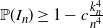 $\mathbb{P}(I_n) \geq 1- c\frac{k_n^4}{n^4}$
.
Proof. We denote the
 $k_n$
column vectors of
 $\Gamma_n$
by
 $\{v_n^i\}_{i=1}^{k_n} \in \mathbb{R}^{n}$
. We say a set of vectors is minimally dependent if any of its proper subsets are linearly independent. For any set of indices of vectors
 $T\subseteq \{1,2,\dots,k_n\}$
we denote
 $V_n^T =\{v_n^i\,{:}\, i\in T\}$
. By noting that
 $I_n^\mathrm{c} = \bigcup_{\ell = 2}^{k_n} \{$
there exists a minimally dependent set of size
 $\ell\}$
, we have
 \begin{equation} \mathbb{P}(I_n^\mathrm{c}) \leq \sum_{\ell=2}^{k_n}\sum_{|T|=\ell}\mathbb{P}(V_n^T \text{ is minimally dependent}) = \sum_{\ell=2}^{k_n}\left(\begin{smallmatrix}k_n\\ 1\end{smallmatrix}\right)\mathbb{P}(B_\ell) , \end{equation}
where
 $B_\ell$
is the event that
 $V_n^T$
is minimally dependent for a particular set T satisfying
 $|T|=\ell$
.
Now fix a set T with
 $|T|=\ell$
. Without loss of generality, let
 $T=\{1,2,\dots,\ell\}$
. Consider a matrix
 $M_\ell$
whose columns are the vectors in
 $V_n^T$
. Note that the set
 $V_n^T$
being minimally dependent implies that
 $M_\ell$
has no row with only one non-zero entry (otherwise, the set of vectors without the column associated with that element would be linearly dependent). This further implies that each non-zero row of
 $M_\ell$
has at least two entries. Since each column of
 $M_\ell$
has exactly four non-zero entries,
 $M_\ell$
has exactly
 $4\ell$
non-zero entries. Therefore, the number of non-zero rows in
 $M_\ell$
must be at most
 $2\ell$
, and the number of zero rows in
 $M_\ell$
must be at least
 $n-2\ell$
. Combining all of the arguments above, we must have
 \begin{align} \mathbb{P}(B_\ell)\leq \mathbb{P}(M_\ell \text{ has at least } n-2\ell \text{ zero rows}). \end{align}
We denote the row vectors of
 $M_\ell$
by
 $\{w_n^i\}_{i=1}^{n}$
. For a subset of indices of species
 $R\subseteq \{1,2,\dots,n\}$
we denote
 $W_n^R=\{w_n^i\,{:}\, i\in R\}$
. We say that
 $W_n^R=0$
if all the vectors in the set are the zero vector. We have
 \begin{equation} \mathbb{P}(M_\ell \text{ has at least } n-2\ell \text{ zero rows}) \leq \sum_{|R|=n-2\ell}\mathbb{P}\big(W_n^R=0\big) =\left(\begin{smallmatrix}n\\ n-2\ell\end{smallmatrix}\right)\mathbb{P}(C_\ell) , \end{equation}
where
 $C_\ell$
is the event that
 $W_n^R=0$
for a particular R satisfying
 $|R|=n-2\ell$
.
Now fix a set R with
 $|R|=n-2\ell$
. Without loss of generality, let
 $R=\{2\ell+1,\dots,n\}$
. Then, the event
 $C_\ell$
involves picking
 $\ell$
column vectors
 $V_n^T=\{v_n^1,\dots,v_n^\ell\}$
where the last
 $n-2\ell$
elements of each column vector are zero. Recall that each column vector has exactly four non-zero elements. Suppose we have already picked j such column vectors. The number of ways we can pick the
 $(j+1)$
st vector is at least
 $\big(\left(\begin{smallmatrix}n\\ 2 \end{smallmatrix}\right)-2j\big)\big(\left(\begin{smallmatrix}n-2\\ 2 \end{smallmatrix}\right) -2j\big)$
(this follows from the same argument as in the proof of Lemma 4.2). Among these, the number of ways we can pick the
 $(j+1)$
st vector whose last
 $n-2\ell$
elements are zero is less than
 $\left(\begin{smallmatrix}2\ell \\ 2\end{smallmatrix}\right) \left(\begin{smallmatrix}2\ell-2 \\ 2\end{smallmatrix}\right)$
. Thus, we have
 \begin{equation*} \mathbb{P}(C_\ell) \leq \prod_{j=0}^{\ell-1} \frac{\left(\begin{smallmatrix}2\ell \\ 2\end{smallmatrix}\right) \left(\begin{smallmatrix}2\ell-2 \\ 2\end{smallmatrix}\right)}{\big(\left(\begin{smallmatrix}n\\ 2 \end{smallmatrix}\right)-2j\big)\big(\left(\begin{smallmatrix}n-2\\ 2 \end{smallmatrix}\right) -2j\big)} \leq \prod_{j=0}^{\ell-1} \frac{\left(\begin{smallmatrix}2\ell \\ 2\end{smallmatrix}\right) \left(\begin{smallmatrix}2\ell-2 \\ 2\end{smallmatrix}\right)}{\frac{1}{4}\left(\begin{smallmatrix}n\\ 2 \end{smallmatrix}\right)\left(\begin{smallmatrix}n-2\\ 2 \end{smallmatrix}\right)} \leq 4 \bigg(\frac{2\ell}{n}\bigg)^4, \end{equation*}
where the second inequality is due to the fact that
 $j\ll n$
. Plugging the above into (4.5), we see that
 \begin{align} \mathbb{P}(M_\ell \text{ has at least } n-2\ell \text{ zero rows}) & \leq \left(\begin{smallmatrix}n\\ n-2\ell\end{smallmatrix}\right)4\bigg(\frac{2\ell}{n}\bigg)^{4\ell} \leq \frac{n^{2\ell}}{(2\ell)!} 4\bigg(\frac{2\ell}{n}\bigg)^{4\ell} \nonumber \\ & \leq \frac{4n^{2\ell}}{\sqrt{2\pi}(2\ell/\mathrm{e})^{2\ell}}\bigg(\frac{2\ell}{n}\bigg)^{4\ell} = \frac{4}{\sqrt{2\pi}\,}\bigg(\frac{2\ell \mathrm{e}}{n}\bigg)^{2\ell}. \end{align}
Now, combining (4.3), (4.4), and (4.6), we have
 \begin{align*} \mathbb{P}(I_n^\mathrm{c}) & \leq \sum_{\ell=2}^{k_n} \left(\begin{smallmatrix}k_n\\[2pt] \ell \end{smallmatrix}\right)\frac{4}{\sqrt{2\pi}\,}\bigg(\frac{2\ell \mathrm{e}}{n}\bigg)^{2\ell}\leq\sum_{\ell=2}^{k_n} \frac{k_n^\ell}{\ell!}\frac{4}{\sqrt{2\pi}\,}\bigg(\frac{2\ell \mathrm{e}}{n}\bigg)^{2\ell} \\[2pt] & \leq \sum_{\ell=2}^{k_n} \frac{k_n^\ell}{\sqrt{2\pi}(\ell/\mathrm{e})^\ell}\frac{4}{\sqrt{2\pi}\,}\bigg(\frac{2\ell \mathrm{e}}{n}\bigg)^{2\ell} =\sum_{\ell=2}^{k_n}\frac{2}{\pi}\bigg(\frac{4\ell \mathrm{e}^3 k_n}{n^2}\bigg)^\ell \\[2pt] & \leq \sum_{\ell=2}^{\infty}\frac{2}{\pi}\bigg(\frac{4 \mathrm{e}^3 k_n^2}{n^2}\bigg)^\ell \leq c \frac{k_n^4}{n^4} \end{align*}
for some constant
 $c>0$
, since
 $k_n\ll n$
. Thus, we have
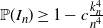 $\mathbb{P}(I_n) \geq 1 - c\frac{k_n^4}{n^4}$
.
We return to the setting of reaction networks with our final key lemma.
Lemma 4.3. Suppose that
 $k_n\ll n$
. Then,
 \begin{equation*} \mathbb{P}(\delta_{R_n}=0 \mid R_n \ \mathrm{is}\ k_n\mathrm{\mbox{-}paired}) \geq \bigg(1-c\frac{k_n^4}{n^4}\bigg)\bigg(1-\frac{21k_n}{n}\bigg). \end{equation*}
Proof. Let
 $R_n$
be a
 $k_n$
-paired reaction network, where
 $k_n\ll n$
. From Lemma 2.1,
 $R_n$
has deficiency zero if and only if all
 $k_n$
reaction vectors are linearly independent. Let
 $I_n$
be the event that all
 $k_n$
reaction vectors are linearly independent.
Similar to Lemma 4.2, denote by
 $A_n$
the event that all reactions have exactly four species. We have
 \begin{align*} \mathbb{P}(\delta_{R_n}=0 \mid R_n \text{ is } \text{$k_n$-paired}) & = \mathbb{P}(I_n \mid R_n \text{ is } \text{$k_n$-paired}) \nonumber \\[2pt] & \geq \mathbb{P}(I_n \mid A_n,R_n \text{ is } \text{$k_n$-paired})\mathbb{P}(A_n \mid R_n \text{ is } \text{$k_n$-paired}). \end{align*}
Utilizing Lemma 4.2 and Proposition 4.1, we complete the proof of Lemma 4.3.
5. Discussion
This work stemmed from a natural question pertaining to reaction networks: given the importance of deficiency zero in the reaction network literature, can we quantify how prevalent the condition is? In the Erdös–Rényi framework we have chosen here, we have provided a threshold function,
 $r(n) = \frac{1}{n^{3}}$
, for the property, in that if
 $p_n \ll r(n)$
then the probability of deficiency zero converges to 1, and if
 $p_n \gg r(n) $
then the probability of deficiency zero converges to 0.
We do not make the claim that the framework selected here is the only, or even the most, biologically relevant. Instead, having equal probabilities for each edge puts as few assumptions on our model as possible, thereby making it a reasonable starting point for analysis. In fact, there are multiple avenues for future research, and we list just a few here.
-
• We may want to study models in which some added structure is known. For example, our assumption of equal probabilities would need to be relaxed in those contexts where different reaction types are more likely to appear in the network than others (such as when inflows and outflows of species are common). This would necessitate the use of a stochastic block model framework. We have carried out such an analysis in [Reference Anderson and Nguyen7].
-
• In the setting of molecular biology, some proteins may be more active and interact with many other proteins, while some proteins may be relatively inactive and have fewer interactions. In such cases, we can study random reaction networks under a more general random graph framework such as the Chung–Lu model, where vertices can be assigned different weights [Reference Chung and Lu10].
-
• Situations can arise in which some species are chemostated, which keeps their concentrations constant. In such a case we may want to focus on the asymptotic behavior of ‘subnetworks’, which consist of the species not being chemostated, instead of the whole network. The study of subnetworks may also be useful in multi-scale settings, where we want to focus on a subset of ‘discrete’ species which have low abundances and behave differently than those in high abundance [Reference Anderson, Cappelletti and Kurtz3].
-
• There are other meaningful topological features beside deficiency zero that we could study with our approach. Some features of interest are deficiency one (together with additional graphical features) as in [Reference Shinar and Feinberg17], endotactic, strongly endotactic, and asyphonic as in [Reference Agazzi, Dembo and Eckmann1, Reference Agazzi, Dembo and Eckmann2, Reference Gopalkrishnan, Miller and Shiu12].
The analysis and methods developed here will, to varying degrees, be applicable to each of the situations listed above.
Acknowledgements
We thank Robin Pemantle for influencing the formulation of the question posed in this paper. We also thank an anonymous reviewer whose comments greatly influenced the final version of this paper.
Funding Information
We gratefully acknowledge grant support from the Army Research Office via grant W911NF-18-1-0324 and the National Science Foundation via grant DMS-2051498.
Competing Interests
There were no competing interests to declare which arose during the preparation or publication process of this article.