



1. Introduction
Liquid–solid two-phase flows are ubiquitous in both natural phenomena, such as alluvial depositions (Fang et al. Reference Fang, Cui, Liu, Zhang, Zhou and Fan2023), landslides (Li et al. Reference Li, Nian, Tiong, Shen and Shao2023a ) and debris flows (Kong & Guan Reference Kong and Guan2023), and industrial processes, including solid waste handling (Zhang et al. Reference Zhang, Okuyama, Higuchi, Soon, Lisak and Law2023) and fluidised beds (Renganathan & Krishnaiah Reference Renganathan and Krishnaiah2004). These systems are characterised by highly nonlinear interphase interactions and interparticle contacts, rendering their accurate modelling a significant challenge.
Extensive experimental investigations have been carried out over decades to elucidate the macroscopic behaviour of liquid–solid flows, particularly focusing on quantities such as bed expansion and the minimum fluidisation velocity. A cornerstone of this effort is the Richardson–Zaki equation, which relates the sedimentation velocity to the fluid volume fraction via a power-law relationship. Originally proposed by Richardson & Zaki (Reference Richardson and Zaki1954) based on experimental data on fluidisation, this relation was later refined by Garside & Al-Dibouni (Reference Garside and Al-Dibouni1977) through modification of the exponent. The resulting correlation has since become widely adopted in drag models for particle-laden flows (Wen & Yu Reference Wen and Yu1966; Syamlal et al. Reference Syamlal, Rogers and O‘Brien1993; Di Felice Reference Di Felice1994). More recent experimental studies have extended this framework to systems involving low-density particles. For instance, Renganathan & Krishnaiah (Reference Renganathan and Krishnaiah2004) examined inverse fluidisation of acrylic particles (with solid densities
 $\rho _s$
ranging from 250 to 917 kg m
 $^{-3}$
) in water, while Nelson et al. (Reference Nelson, Srabet, Nan, Pjontek and Zhu2022) measured the minimum fluidisation velocity of Styrofoam particles and proposed a modified Wen–Yu correlation. Similarly, Nan & Zhu (Reference Nan and Zhu2022) investigated hydrodynamics in an inverse liquid–solid circulating fluidised bed (CFB) using polystyrene particles in salt water, observing deviations from homogeneity and introducing a revised Richardson–Zaki formulation. In another application, Lv et al. (Reference Lv, Zhao, Deng, Fang, Xing and Dong2021) studied fluidised granular activated carbon for copper ion removal from wastewater.
Complementing experimental efforts, numerical simulations offer detailed insights into the structures of these flows. Two-fluid models (TFM), for example, have been employed to capture bulk hydrodynamic features. Wang et al. (Reference Wang, Sun, Yang, Zhao, Gao and Liu2014) simulated inverse liquid–solid fluidisation using the Huilin–Gidaspow drag model and noted that predicted bed expansion slightly exceeded experimental measurements, a discrepancy suggesting the need for drag correlations that explicitly account for the particle–fluid density ratio
 $\rho ^\ast =\rho _s/\rho _{\!f}$
, where
 $\rho _{\!f}$
denotes the fluid density. Song et al. (Reference Song, Zhu, Zhang, Sun and Lu2019) further applied TFM to both upward and downward CFBs, reporting similar distributions of particle concentration and velocity in the two configurations.
However, conventional TFM formulations rely on constitutive relations derived from kinetic theory for granular flows (KTGF) (Jenkins & Savage Reference Jenkins and Savage1983; Lun et al. Reference Lun, Savage, Jeffrey and Chepurniy1984; Sinclair & Jackson Reference Sinclair and Jackson1989; Louge et al. Reference Louge, Mastorakos and Jenkins1991; Gidaspow Reference Gidaspow1994), which were originally developed for dry granular systems and neglect the influence of the interstitial fluid phase. While the liquid-phase turbulence is often modelled using the
 $k-\epsilon$
turbulence model equations, particle–turbulence interactions remain neglected. The solid pressure
 $p_s$
model proposed by Lun et al. (Reference Lun, Savage, Jeffrey and Chepurniy1984), for instance, depends on the radial distribution function (RDF) at contact,
 $\chi$
, and the restitution coefficient,
 $e$
, to describe inelastic collisions. Values of
 $\chi$
are typically obtained from experiments on dry granular media (Gidaspow & Huilin Reference Gidaspow and Huilin1998) or molecular dynamics simulations (Ma & Ahmadi Reference Ma and Ahmadi1986), yet such approaches fail to reproduce the anisotropic microstructures observed in liquid–solid suspensions (Yin & Koch Reference Yin and Koch2007; Willen & Prosperetti Reference Willen and Prosperetti2019). Moreover, lubrication interactions arising from the thin interstitial fluid films between closely approaching particles introduce additional dissipation beyond that present in dry granular flows (Gao et al. Reference Gao, Liu, Guo and Lu2022), thereby altering collision dynamics. The viscous dissipation stemming from interphase momentum exchange plays a crucial role in flow instabilities (Koch Reference Koch1990; Garzó Reference Garzó2005; Yin et al. Reference Yin, Zenk, Mitrano and Hrenya2013), indicating that existing models – such as the viscous dissipation term for dilute gas–solid flows by Louge et al. (Reference Louge, Mastorakos and Jenkins1991) and the collisional dissipation model for inelastic granular materials by Jenkins & Savage (Reference Jenkins and Savage1983) – are inadequate for liquid–solid systems.
Particle-resolved direct numerical simulation (PR-DNS) offers a more fundamental approach by solving the hydrodynamic (Willen & Prosperetti Reference Willen and Prosperetti2019; Wang & Hu Reference Wang and Hu2025) or kinetic (Yin & Koch Reference Yin and Koch2007; Rubinstein et al. Reference Rubinstein, Derksen and Sundaresan2016; Fullmer et al. Reference Fullmer, Liu, Yin and Hrenya2017) equations for the fluid phase and Newton’s equations for individual particles, with no-slip boundary conditions enforced at particle surfaces. This method yields fully resolved interphase interactions without empirical closures, as the fluid stress tensor is integrated directly over particle boundaries. Consequently, PR-DNS has become pivotal for constructing particle–fluid interaction models. For instance, Lattanzi et al. (Reference Lattanzi, Tavanashad, Subramaniam and Capecelatro2022) developed a force Langevin model for particle–fluid interactions based on PR-DNS data, whilst recent work by Wang & Hu (Reference Wang and Hu2025) proposed a stochastic drag model in particle-laden turbulence.
Over the past decade, PR-DNS has been extensively employed to investigate particle suspensions across a wide spectrum of particle–fluid density ratios (
 $\rho ^\ast$
), revealing profound effects on flow structures and particle dynamics. For neutrally buoyant suspensions (
 $\rho ^\ast =1$
), PR-DNS studies have elucidated the modulation of wall turbulence by finite-size particles. For instance, Zhu et al. (Reference Zhu, Yu and Shao2018) and Eshghinejadfa et al. (Reference Eshghinejadfa, Zhao and Thévenin2018) demonstrated that non-spherical neutrally buoyant particles can induce significant drag reduction in turbulent channel flows by altering near-wall streaks and suppressing Reynolds shear stress. When the density ratio deviates from unity, the interplay between particle inertia, buoyancy and fluid turbulence leads to complex migration and clustering behaviours. Xia et al. (Reference Xia, Yu and Guo2020) investigated particle-laden turbulent channel flows with spanwise rotation, revealing that heavy particles (
 $\rho ^\ast \gt 1$
) migrate towards the pressure wall, whereas light particles (
 $\rho ^\ast \lt 1$
) migrate towards the suction wall, driven by mean secondary flow structures. For settling suspensions (
 $\rho ^\ast \gt 1$
), PR-DNS has provided critical insights into particle clustering, microstructures and pseudoturbulence. Jiang et al. (Reference Jiang, Xu and Zhao2024) and Jiang et al. (Reference Jiang, Brandt, Xu and Zhao2025) showed that settling spheroids form column-like clusters due to wake-induced hydrodynamic interactions, which enhances the mean settling velocity and induces anisotropic pseudoturbulence. Furthermore, Zhu et al. (Reference Zhu, Yu, Pan and Shao2020) and Xia et al. (Reference Xia, Lin, Guo and Yu2024) highlighted the significant effects of particle shape and mesoscale clustering on the flow friction and filtered drag force in upward vertical flows and clustered settling suspensions. In addition to dynamic suspensions, PR-DNS of flow past fixed or rotating particle arrays has been instrumental in formulating accurate hydrodynamic force correlations for both spherical and non-spherical particles across various Reynolds numbers and solid volume fractions (Zhou & Fan Reference Zhou and Fan2015a
,
Reference Zhou and Fanb
; Li et al. Reference Li, Chen, Yang and Zhou2023b
).
In practice, gas–solid flows are often simplified as flows through fixed particle arrays owing to slow response and corresponding high Stokes numbers of inertial particles, whereas liquid–solid flows are characterised as sedimenting suspensions, equivalent to fluidisations under a Galilean transformation. Fullmer et al. (Reference Fullmer, Liu, Yin and Hrenya2017) compared PR-DNS data with TFM simulations based on the Garzó–Tenneti–Subramaniam–Hrenya (GTSH) model (Garzó et al. Reference Garzó, Tenneti, Subramaniam and Hrenya2012) for density ratios
 $\rho ^\ast$
between 2 and 1000, finding significant deviations when the high thermal Stokes number assumption breaks down.
The thermal Stokes number is defined as the ratio of the particle–fluid viscous dissipation relaxation time to the mean particle–particle collision time; a high value implies that fluid-mediated dissipation is negligible compared with collisional effects. Moreover, both Yin & Koch (Reference Yin and Koch2007) and Willen & Prosperetti (Reference Willen and Prosperetti2019) reported pronounced anisotropy of particle arrangements in liquid–solid suspensions, which is a feature absent in the isotropic GTSH framework. The non-exponential decay of the particle velocity autocorrelation function (ACF), as observed by Willen & Prosperetti (Reference Willen and Prosperetti2019), also challenges the Langevin-type stochastic assumption underpinning the GTSH model.
Despite these insights, the development of particle–fluid interaction models in liquid–solid flows, particularly those valid across broad density-ratio ranges, remains inadequate. Zaidi (Reference Zaidi2018) proposed a drag law dependent on particle inertia for particle concentration
 $\phi \leqslant 0.2$
, while Tavanashad et al. (Reference Tavanashad, Passalacqua and Subramaniam2021) developed a drag correlation in terms of the particle Reynolds number
 $\textit{Re}$
, particle concentration
 $\phi$
and particle–fluid density ratio
 $\rho ^\ast$
. However, both studies explored only a limited range of
 $\rho ^\ast$
, insufficient to capture the trends identified by Fullmer et al. (Reference Fullmer, Liu, Yin and Hrenya2017) across broader density contrasts. It is important to note that the study of Fullmer et al. (Reference Fullmer, Liu, Yin and Hrenya2017) was restricted to heavy, settling particles (
 $\rho ^\ast \geqslant 2$
). The floating (
 $\rho ^\ast \lt 1$
) and near-neutral-buoyancy (
 $\rho ^\ast \approx 1$
) regimes, which are prevalent in applications such as inverse fluidisation and neutrally buoyant suspensions, remain essentially unexplored by particle-resolved simulations. A systematic quantification of the KTGF closures and the role of particle–fluid density ratio over a wide range is still lacking.
In this work, we perform PR-DNS of fully periodic liquid–solid suspensions to extend the parameter space of Fullmer et al. (Reference Fullmer, Liu, Yin and Hrenya2017), who considered density ratios
 $\rho ^\ast$
between 2 and 1000. By including
 $\rho ^\ast$
as low as 0.05, we span the full range from floating (
 $\rho ^\ast \lt 1$
) through near-neutral buoyancy (
 $\rho ^\ast \approx 1$
) to settling (
 $\rho ^\ast \gt 1$
) particles. This extension is essential because the floating and neutrally buoyant regimes are relevant to inverse fluidisation and many environmental flows (Song et al. Reference Song, Zhu, Zhang, Sun and Lu2019), yet they have received little attention in PR-DNS studies. Moreover, the lower
 $\rho ^\ast$
values magnify the role of fluid inertia and virtual mass forces, which are negligible in the high-density-ratio limit of Fullmer et al. (Reference Fullmer, Liu, Yin and Hrenya2017). Consequently, the present dataset reveals density-ratio effects on the Richardson–Zaki exponent, on the granular temperature, and on the collisional transport that could not be observed in the earlier work. This allows us to systematically explore the influence of particle–fluid density ratio on suspension dynamics. A further objective is to quantify correlations proposed in KTGF models, e.g. the RDF at contact
 $\chi$
and the solid pressure
 $p_s$
, and to examine quantitatively deviations from the Maxwell velocity distribution. To ensure statistical convergence, sufficiently long time series are simulated, guided by the ACF results reported by Willen & Prosperetti (Reference Willen and Prosperetti2019).
This paper is organised as follows. Section 2 outlines the lattice Boltzmann method (LBM) developed by Ladd (Reference Ladd1994a
,Reference Ladd
b
), describes the simulation set-up, specifies the parameter ranges and introduces the statistical tools and mathematical notation used throughout. In § 3.3, we establish dependence on
 $\rho ^\ast$
of the exponent
 $n$
and the prefactor
 $k$
in the modified Richardson–Zaki equation for both terminal Reynolds numbers. Section 3.4 investigates particle velocity fluctuations through the granular temperature, the second and third invariants, and the skewness and kurtosis (the third and fourth moments). The ACF and partial ACF (PACF) of particle velocity are analysed in § 3.5 to quantify the contribution of interstitial fluid to particle random motion. Section 3.6 presents the pair correlation function (PCF) to characterise the anisotropic spatial microstructure, together with quantification of the RDF at contact
 $\chi$
, which represents the collision frequency. In § 3.7, we compute collisional solid pressure and dissipation, which is compared with predictions of KTGF models. Section 3.8 examines the divergence of local spatial averaged solid-phase velocity, which provides another measure of spatial fluctuations. Finally, key findings are summarised in § 4.
2. Methods
2.1. The PR-DNS method
We conduct PR-DNS using the Susp3D code (Ladd Reference Ladd1994a , Reference Laddb ). The fluid phase is governed by the incompressible Navier–Stokes equations,
 \begin{align} \boldsymbol{\nabla \boldsymbol{\cdot }u} &= 0, \\[-12pt]\nonumber \end{align}
 \begin{align} \frac {\partial \boldsymbol{u}}{\partial t} + \boldsymbol{u\boldsymbol{\cdot }\boldsymbol{\nabla }u} &= -\frac {1}{\rho _{\!f}}\boldsymbol{\nabla }\!p + \nu _{\!f}{\nabla} ^2\boldsymbol{u} + \boldsymbol{g}, \end{align}
where
 $\boldsymbol{u}$
is the fluid velocity,
 $p$
is the pressure,
 $\nu _{\!f}$
is the kinematic viscosity and
 $\boldsymbol{g}$
is gravity. The fluid equations are solved using the D3Q19 LBM with a two-relaxation-time model. The evolution of the distribution functions follows the lattice Boltzmann equations with the two-relaxation-time collision operator; the detailed information can be found in Ladd (Reference Ladd1994a
,Reference Ladd
b
).
The motion of the
 $p$
th rigid spherical particle is governed by Newton’s equations for translation and rotation,
 \begin{align} m_{\!p}\frac {\mathrm{d}\boldsymbol{v}_p}{\mathrm{d}t} &= \boldsymbol{F}_{\!p}^h + \sum _{q}\boldsymbol{F}_{\!pq}^c + m_{\!p}\boldsymbol{g}, \\[-12pt]\nonumber \end{align}
 \begin{align} I_{\!p}\frac {\mathrm{d}\boldsymbol{\omega }_p}{\mathrm{d}t} &= \boldsymbol{T}_{\!p}^h + \sum _{q}\boldsymbol{T}_{\!pq}^c, \end{align}
where
 $m_{\!p}$
and
 $I_{\!p}$
are the mass and moment of inertia of the
 $p$
th particle,
 $\boldsymbol{v}_p$
and
 $\boldsymbol{\omega }_p$
are its translational and angular velocities,
 $\boldsymbol{F}_{\!p}^h$
and
 $\boldsymbol{T}_{\!p}^h$
are the hydrodynamic force and torque exerted by the fluid, and
 $\boldsymbol{F}_{\!pq}^c$
and
 $\boldsymbol{T}_{\!pq}^c$
are the force and torque due to interparticle collisions by the
 $q$
th particle. The hydrodynamic force and torque are, respectively, defined by
 \begin{align} \boldsymbol{F}_{\!p}^h &= \iint _{S_p}\boldsymbol{\sigma \boldsymbol{\cdot }n}\mathrm{d}S, \\[-12pt]\nonumber \end{align}
 \begin{align} \boldsymbol{T}_{\!p}^h &= \iint _{S_p} (\boldsymbol{x}-\boldsymbol{x}_{\!p} ) \times \left (\boldsymbol{\sigma \boldsymbol{\cdot }n}\right )\mathrm{d}S, \end{align}
where
 $S_p$
is the surface of the particle,
 $\boldsymbol{\sigma }=-p{\unicode{x1D644}}+\mu _{\!f}[\boldsymbol{\nabla u}+(\boldsymbol{\nabla u})^T]$
is the total stress tensor,
 $\boldsymbol{n}$
is the unit outward normal vector on the particle surface,
 $\boldsymbol{x}$
is the variable of integration and
 $\boldsymbol{x}_{\!p}$
is the centre of the particle. The no-slip boundary condition is imposed on the particle surfaces via the bounce-back scheme. The hydrodynamic force and torque are computed by accumulating the momentum exchange between the fluid and the particle across the surface links (Ladd Reference Ladd1994a
,
Reference Laddb
).
We model interparticle collisions via a hard-sphere collision model. During each lattice time step, all potential pairwise collisions are iteratively identified and used to update postcollision velocities. The collisions are binary and instantaneous, characterised by a normal restitution coefficient
 $e$
. When two particles are in near contact, the fluid flow in the gap cannot be resolved by the grid (Nguyen & Ladd Reference Nguyen and Ladd2002). Therefore, a lubrication correction is required to account for the unresolved hydrodynamic interactions. We adopt the analytical lubrication model and its implementation described in Nguyen & Ladd (Reference Nguyen and Ladd2002), which is applied when the surface-to-surface distance between two particles is smaller than a threshold
 $h_c = 0.01d_p$
. This threshold is chosen following Nguyen & Ladd (Reference Nguyen and Ladd2002) and Fullmer et al. (Reference Fullmer, Liu, Yin and Hrenya2017). This correction ensures accurate particle dynamics at small separations.
The terminal velocity of an isolated settling particle
 $v_t$
defines the terminal Reynolds number (
 $\textit{Re}_t=\rho _{\!f}v_td_p/\mu _{\!f}$
), where
 $\rho _{\!f}$
is the fluid density,
 $d_p$
is the particle diameter and
 $\mu _{\!f}$
is the dynamic viscosity of the fluid. Grid independence is maintained across varying
 $\textit{Re}_t$
, by adjusting
 $d_p$
in lattice units. For
 $\textit{Re}_t=3$
, the particle diameter is
 $d_p=5.84$
lattice units, and for
 $\textit{Re}_t=30$
,
 $d_p=6.354$
lattice units. These resolutions correspond to at least
 $5.84$
grid points per particle diameter, which is known to be sufficient for the accurate computation of hydrodynamic forces and lubrication interactions in the LBM framework (Fullmer et al. Reference Fullmer, Liu, Yin and Hrenya2017). The other physical parameters (fluid density, viscosity and system size relative to
 $d_p$
) are chosen to match the benchmark cases of Fullmer et al. (Reference Fullmer, Liu, Yin and Hrenya2017), so that the present results can be validated against their data in the overlapping density-ratio range. This choice does not imply an identical simulation; the density ratio, gravity and resulting flow dynamics are markedly different across the extended parameter space. Particles are not perfectly spherical due to the staircase approximation inherent in the bounce-back scheme, leading to an effective hydrodynamic diameter
 $d_p$
, which differs from the geometric diameter
 $d_p^0$
. The hydrodynamic correction is thus defined as
 $\Delta _d=d_p-d_p^0$
. This procedure is standard in LBM simulations of spherical particles (Ladd Reference Ladd1994a
,
Reference Laddb
) and has been shown to yield correct hydrodynamic forces and torques, with the asphericity effects being negligible for the Reynolds numbers considered here. Table 1 summarises simulation parameters in lattice units.
Simulation parameters for terminal Reynolds numbers
 $\textit{Re}_t=3$
and
 $\textit{Re}_t=30$
in lattice units.

Table 1. Long description
A table comparing simulation parameters for terminal Reynolds numbers of 3 and 30. The table has 6 rows and 3 columns. Column headers are Archimedes number, Particle diameter, Fluid density, Fluid viscosity, Fluid relaxation time, and Hydrodynamic correction. Row 1: Archimedes number, Ar, 71.03, 1432. Row 2: Particle diameter, d p, 5.84, 6.354. Row 3: Fluid density, ρ f, 36, 36. Row 4: Fluid viscosity, μ f, 0.36, 0.03. Row 5: Fluid relaxation time, τ f, 0.53, 0.5025. Row 6: Hydrodynamic correction, Δ d, 0.224, 0.477.
To ensure statistical significance, we run simulations for 1 000 000 and 1 600 000 lattice time steps for
 $\textit{Re}_t=3$
and
 $\textit{Re}_t=30$
, respectively. These time steps are estimated using the autocorrelation results reported by Willen & Prosperetti (Reference Willen and Prosperetti2019), which ensure at least 100 independent samples for each case. Data are saved every 100 and 200 time steps to optimise storage.
2.2. System description
The system comprises monodisperse rigid spheres suspended in an incompressible Newtonian fluid. Periodic boundary conditions are imposed in all directions, which keeps
 $\phi$
a constant. Particles are initially randomly distributed with zero overlap. A constant body force (gravity
 $\boldsymbol{g}$
) in the y direction induces relative motions between the two phases. In a real, unbounded suspension, gravity would be balanced by a macroscopic pressure gradient that supports the weight of the mixture and is physically equivalent to the buoyancy force acting on the mixture. Because our domain is triply periodic, a net pressure gradient cannot develop spontaneously; the flow would otherwise accelerate indefinitely. To reproduce the physical stress state, we therefore impose a mean fluid pressure gradient
 $\langle \partial P_{\!f}/\partial y\rangle$
that exactly balances the total weight of the suspension,
 \begin{equation} -\left \langle \frac {\partial P_{\!f}}{\partial y}\right \rangle = \left [\rho _{\!f}(1-\phi )+\rho _s\phi \right ]g, \end{equation}
where
 $\langle \boldsymbol{\cdot }\rangle$
denotes the spatial average over the entire computational domain (the formal definition is given in § 2.3 by (2.22)),
 $\phi =({\pi }/{6})d_p^3N_{\!p}/V$
is the mean particle concentration defined by the ratio of the particle-phase volume to the entire domain volume
 $V$
,
 $\rho _s$
is particle density and
 $g=|\boldsymbol{g}|$
is the magnitude of gravitational acceleration. Thus, the net force acting on the system is zero in each direction.
To maintain the low-Mach-number assumption of LBM, where smaller macroscopic velocity magnitude would ensure higher precision, we set the superficial mixture velocity to zero by
 \begin{equation} \phi \boldsymbol{U}_{\!s} + (1-\phi )\boldsymbol{U_{\!f}} = \boldsymbol{0}, \end{equation}
where
 $\boldsymbol{U}_{\!s}$
and
 $\boldsymbol{U_{\!f}}$
denote the mean velocities of particle and fluid phase, respectively. This Galilean transformation to a frame with zero mixture velocity does not alter the relative motion between the phases; the particle–fluid interactions and all statistical quantities of interest remain unchanged. Thus, drift velocity
 $\boldsymbol{U_d}$
, defined as relative velocity
 $\boldsymbol{U}_{\!r}=\boldsymbol{U}_{\!s}-\boldsymbol{U_{\!f}}$
multiplied by mean fluid volume fraction
 $(1-\phi )$
, equals to the mean solid velocity
 $\boldsymbol{U}_{\!s}$
,
 \begin{equation} \boldsymbol{U_d} = (1-\phi )\left (\boldsymbol{U}_{\!s}-\boldsymbol{U_{\!f}}\right ) = \boldsymbol{U}_{\!s}. \end{equation}
Here,
 $\boldsymbol{U_{\!f}}$
and
 $\boldsymbol{U}_{\!s}$
are obtained from the simulation by volume averaging over the respective phases and time averaging after the flow reaches a statistically steady state. It is important to note that
 $\boldsymbol{U_{\!f}}$
is not zero; its value is determined by the dynamic balance of gravity, the imposed pressure gradient (buoyancy) and the interphase momentum exchange (e.g. drag).
The particle Reynolds number is defined as
 \begin{equation} \textit{Re} = \frac {\rho (1-\phi )|\boldsymbol{U}_{\!s}-\boldsymbol{U_{\!f}}|d_p}{\mu _{\!f}} = \frac {\rho |\boldsymbol{U}_{\!s}|d_p}{\mu _{\!f}}. \end{equation}
This system is characterised by seven dimensionless parameters: Archimedes number,
 $Ar=\rho _{\!f}|(\rho _s-\rho _{\!f})g|d_p^3/\mu _{\!f}^2$
; particle–fluid density ratio,
 $\rho ^\ast =\rho _s/\rho _{\!f}$
; mean particle concentration,
 $\phi$
; restitution coefficient of interparticle collisions,
 $e$
; and relative system size in each direction,
 $L_j^\ast =L_j/d_p$
, where
 $j=x,y,z$
.
The Archimedes number
 $Ar$
quantifies gravity-to-viscous force ratio and is uniquely determined by
 $\textit{Re}_t$
(Yin & Koch Reference Yin and Koch2007),
 \begin{equation} Ar = \left \{\begin{array}{ll} 18\textit{Re}_t\big [1+0.1315\textit{Re}_t^{(0.82-0.05\log _{10}\textit{Re}_t)}\big ], & 0.01\lt \textit{Re}_t\lt 20, \\[5pt] 18\textit{Re}_t\big (1+0.1935\textit{Re}_t^{0.6305}\big ), & 20\lt \textit{Re}_t\lt 260. \end{array}\right . \end{equation}
As shown in table 1,
 $\textit{Re}_t=3$
and
 $\textit{Re}_t=30$
cases are investigated, where
 $Ar=71.03$
and 1432, respectively. For each combination of
 $\rho ^\ast$
and
 $\textit{Re}_t$
, the magnitude of gravitational acceleration
 $g$
is uniquely determined from the definition
 $Ar = \rho _{\!f} |(\rho _s - \rho _{\!f})g| d_p^3/\mu _{\!f}^2$
, using the value of
 $Ar$
obtained from (2.11) for the chosen
 $\textit{Re}_t$
. Consequently, the prescribed Archimedes number is exactly achieved in the simulations irrespective of
 $\rho ^\ast$
. The sign of
 $g$
is then set positive for
 $\rho ^\ast \gt 1$
and negative for
 $\rho ^\ast \lt 1$
to ensure that the steady mean particle velocity is directed along the positive
 $y$
axis. We investigate density ratios
 $\rho ^\ast =\{0.05,0.9,1.2,1.8,2.5,5.5\}$
, covering three regimes: floating (
 $\rho ^\ast \lt 1$
); near-neutral-buoyant (
 $\rho ^\ast \approx 1$
); settling (
 $\rho ^\ast \gt 1$
) particles. Specifically,
 $\rho ^\ast =0.05$
and 0.9 are chosen to represent floating behaviours of particles, such as inverse fluidisation (Renganathan & Krishnaiah Reference Renganathan and Krishnaiah2004; Song et al. Reference Song, Zhu, Zhang, Sun and Lu2019; Nan & Zhu Reference Nan and Zhu2022). Near-neutral-buoyant particles are represented by
 $\rho ^\ast =0.9$
, 1.2 and 1.8, which correspond to materials with comparable densities to the fluid, such as granular activated carbon (Lv et al. Reference Lv, Zhao, Deng, Fang, Xing and Dong2021) and polyformaldehyde particles (Jiang et al. Reference Jiang, Shen, Qi, Jing, Li, Yare and Li2021). Here
 $\rho ^\ast =2.5$
represents the typical glass–water density ratio. Heavy materials, such as copper and zirconia, employed as particle electrodes (Cheng et al. Reference Cheng, Yang, Li, Hu, Yu and Li2022) are represented by
 $\rho ^\ast =5.5$
. For convenience, we set
 $g$
positive for
 $\rho ^\ast \gt 1$
and negative for
 $\rho ^\ast \lt 1$
, to keep the steady mean particle velocity positive in the y direction. Notably, it is the density difference and gravity that drive the motion of the suspensions. The particles and the fluid would maintain stationary, if
 $\rho ^\ast =1$
. Thus, the conclusions of this study may not apply to neutrally buoyant particles (
 $\rho ^\ast =1$
).
We adopt system sizes from Fullmer et al. (Reference Fullmer, Liu, Yin and Hrenya2017), with
 $L_x^\ast =L_z^\ast$
for statistical axisymmetry and
 $L_y^\ast =4L_x^\ast$
to resolve particle wakes. We acknowledge that the present domain size (
 $L_x^\ast \approx 8.56$
) is modest when compared with the scale required to eliminate all periodic boundary artefacts in unbounded suspensions. The dimensions were chosen to match the validated benchmark cases of Fullmer et al. (Reference Fullmer, Liu, Yin and Hrenya2017), thereby ensuring that the vertical extent (
 $L_y^\ast = 4L_x^\ast$
) is sufficient to resolve particle wakes and that the results remain directly comparable to existing data. Carrying out direct numerical simulation in substantially larger systems is not computationally feasible for the parameter space investigated here (six density ratios, four concentrations and two restitution coefficients at two terminal Reynolds numbers). We therefore regard the present simulations in this smaller, carefully controlled system as a necessary and reasonable first step in isolating the density-ratio effects on local particle–fluid interactions and suspension microstructure. In our system, the
 $x$
and
 $z$
components of the vectors in the results can be treated as independently and identically distributed samples, simplifying the analysis. Specific values for
 $L_x^\ast$
are 8.562 at
 $\textit{Re}_t=3$
and 8.656 at
 $\textit{Re}_t=30$
. Four mean particle concentrations
 $\phi$
are employed: 0.1, 0.15, 0.25 and 0.4. The corresponding numbers of particles
 $N_{\!p}$
are listed in table 2. To investigate the effect of inelastic collisions, two restitution coefficients, 0.9 and 1.0, are employed. Five independent initial configurations ensure statistical independence.
Particle numbers
 $N_{\!p}$
for mean particle concentrations
 $\phi$
at
 $\textit{Re}_t=3$
and
 $\textit{Re}_t=30$
.

Table 2. Long description
A table comparing particle numbers for mean particle concentrations at Reynolds numbers 3 and 30. The table has four rows and three columns. The columns are labeled with Reynolds numbers 3 and 30, and the row labels are phi values: 0.1, 0.15, 0.25, and 0.4. Row 1: phi = 0.1, 479, 495. Row 2: phi = 0.15, 719, 743. Row 3: phi = 0.25, 1199, 1239. Row 4: phi = 0.4, 1918, 1982.
2.3. Statistical tools
This section presents the mathematical framework for statistical analysis. To investigate the structure of the flow field, we employ the volume filter method proposed by Capecelatro & Desjardins (Reference Capecelatro and Desjardins2013), a further development of the local spatial average method introduced by Anderson & Jackson (Reference Anderson and Jackson1967) and Jackson (Reference Jackson2000). The volume-filtered value of an arbitrary phase-
 $i$
quantity
 $\mathcal{F}$
is defined as
 \begin{equation} \varepsilon _i(\boldsymbol{x},t)\langle \mathcal{F}\rangle ^i(\boldsymbol{x},t) = \iiint _{V_i}\mathcal{F}(\boldsymbol{y},t)G(|\boldsymbol{x}-\boldsymbol{y}|) \mathrm{d}V_{\!y}, \end{equation}
where
 $G(r)$
is the kernel function,
 $V_i$
is the volume occupied by phase-
 $i$
and
 $\langle \boldsymbol{\cdot }\rangle ^i$
denotes the volume filter operator for phase-
 $i$
. For the discrete phase, we assume that
 $\mathcal{F}$
varies little over
 $V_i$
, allowing us to simplify (2.12) into
 \begin{equation} \varepsilon _s(\boldsymbol{x},t)\langle \mathcal{F}\rangle ^s(\boldsymbol{x},t) = V_p\sum _p\mathcal{F}(\boldsymbol{y}_{\!p},t)G(|\boldsymbol{x}-\boldsymbol{y}_{\!p}|), \end{equation}
where
 $\boldsymbol{y}_{\!p}$
is the coordinate of particle
 $p$
, and
 $V_p$
is its volume.
The local (or volume-filtered) particle concentration
 $\varepsilon _s$
and local solid velocity
 $\boldsymbol{u_s}$
are obtained by setting
 $\mathcal{F}=1$
and
 $\mathcal{F}=\boldsymbol{v_p}$
in (2.13), respectively,
 \begin{equation} \varepsilon _s(\boldsymbol{x},t) = V_p\sum _{p}G(|\boldsymbol{x}-\boldsymbol{y}_{\!p}|), \end{equation}
and
 \begin{equation} \varepsilon _s(\boldsymbol{x},t)\boldsymbol{u_s}(\boldsymbol{x},t) = V_p\sum _p\boldsymbol{v_p}G(|\boldsymbol{x}-\boldsymbol{y}_{\!p}|), \end{equation}
where
 $\boldsymbol{v_p}$
is the velocity of particle
 $p$
.
To ensure differentiability and smoothness, we employ the Gaussian kernel function
 \begin{equation} G(r) = \frac {1}{(2\pi )^{3/2}\sigma ^3}e^{-\frac {r^2}{2\sigma ^2}}, \end{equation}
where
 $\sigma$
is the bandwidth, which should satisfy the scale separation assumption. Namely,
 $\sigma$
should be large enough to recover the appropriation in (2.13) and align with classic drag models, yet small enough to preserve mesoscale structures. Capecelatro & Desjardins (Reference Capecelatro and Desjardins2013) suggest that for monodisperse systems, the filter length should be proportional to several particle diameters and recommend
 $\sigma =3d_p/\sqrt {2\ln 2}\approx 2.548d_p$
.
Using (2.14) and (2.16), the gradient of
 $\varepsilon _s$
is defined as
 \begin{eqnarray} \boldsymbol{\nabla }\varepsilon _s(\boldsymbol{x},t) &=& V_p\sum _p\boldsymbol{\nabla }G(|\boldsymbol{x}-\boldsymbol{y}_{\!p}|) \nonumber \\&=& -\frac {V_p}{\sigma ^2}\sum _p\big (\boldsymbol{x}-\boldsymbol{y}_{\!p}\big ) G(|\boldsymbol{x}-\boldsymbol{y}_{\!p}|). \end{eqnarray}
The gradient of left-hand side of (2.13) is
 \begin{eqnarray} \boldsymbol{\nabla }\left (\varepsilon _s(\boldsymbol{x},t) \langle \mathcal{F}\rangle ^s(\boldsymbol{x},t)\right ) &=& \boldsymbol{\nabla }\left [V_p\sum _p\mathcal{F}(\boldsymbol{y}_{\!p},t) G(|\boldsymbol{x}-\boldsymbol{y}_{\!p}|)\right ] \nonumber \\&=& V_p\sum _p\mathcal{F}(\boldsymbol{y}_{\!p},t)\boldsymbol{\nabla }G(|\boldsymbol{x}-\boldsymbol{y}_{\!p}|) \nonumber \\&=& -\frac {V_p}{\sigma ^2}\sum _p \mathcal{F}(\boldsymbol{y}_{\!p},t) \big (\boldsymbol{x}-\boldsymbol{y}_{\!p}\big)G(|\boldsymbol{x}-\boldsymbol{y}_{\!p}|). \end{eqnarray}
Combining (2.17) and (2.20), the explicit definition of gradient of
 $\langle \mathcal{F}\rangle ^s(\boldsymbol{x},t)$
is given by
 \begin{eqnarray} \boldsymbol{\nabla }\langle \mathcal{F}\rangle ^s(\boldsymbol{x},t) &=& \frac {1}{\varepsilon _s} \left [\boldsymbol{\nabla }\left (\varepsilon \langle \mathcal{F}\rangle ^s(\boldsymbol{x},t)\right ) -\left (\boldsymbol{\nabla }\varepsilon _s\right )\langle \mathcal{F}\rangle ^s(\boldsymbol{x},t)\right ] \nonumber \\ &=&\frac {-V_p}{\varepsilon _s\sigma ^2}\sum _p \left (\mathcal{F}(\boldsymbol{y}_{\!p},t)-\langle \mathcal{F}\rangle ^s(\boldsymbol{x},t)\right ) \left (\boldsymbol{x}-\boldsymbol{y}_{\!p}\right ) G\left (|\boldsymbol{x}-\boldsymbol{y}_{\!p}|\right )\!. \end{eqnarray}
Applying this to
 $\mathcal{F}=\boldsymbol{v_p}$
, we obtain the gradient and divergence of
 $\boldsymbol{u_s}$
:
 \begin{equation} \boldsymbol{\nabla u_s} =-\frac {V_p}{\varepsilon _s\sigma ^2} \sum _p\big (\boldsymbol{v_p}-\boldsymbol{u_s}\big ) \big (\boldsymbol{x}-\boldsymbol{y}_{\!p}\big ) G\big (|\boldsymbol{x}-\boldsymbol{y}_{\!p}|\big ), \end{equation}
and
 \begin{equation} \boldsymbol{\nabla \boldsymbol{\cdot }u_s} =-\frac {V_p}{\varepsilon _s\sigma ^2} \sum _p\big (\boldsymbol{v_p}-\boldsymbol{u_s}\big ) \boldsymbol{\cdot }\big (\boldsymbol{x}-\boldsymbol{y}_{\!p}\big ) G\big (|\boldsymbol{x}-\boldsymbol{y}_{\!p}|\big ). \end{equation}
When
 $G(r)$
is taken as a uniform kernel over the whole domain, the volume filter reduces to the spatial average over the entire system. For any field
 $\mathcal{F}$
of the fluid phase, this average is defined as
 \begin{equation} \langle \mathcal{F}\rangle (t) = \frac {1}{(1-\phi )V}\iiint _{V_{\!f}}\mathcal{F}(\boldsymbol{y},t) \mathrm{d}V_{\!y}, \end{equation}
while for any quantity
 $\mathcal{F}(t)$
of the particle phase, it is given by
 \begin{equation} \langle \mathcal{F}\rangle \left (t\right ) = \frac {1}{N_{\!p}}\sum _p\mathcal{F}_p\left (t\right ), \end{equation}
where
 $\mathcal{F}_p$
is the property of particle
 $p$
. The unbiased variance and standard deviation are defined as
 \begin{align} \mathrm{Var}(\mathcal{F}) &= \frac {1}{N_{\!p}-1}\sum _{p} \left (\mathcal{F}-\langle \mathcal{F}\rangle \right )^2\!, \\[-12pt]\nonumber \end{align}
 \begin{align} \mathrm{Std}(\mathcal{F}) &= \sqrt {\mathrm{Var}(\mathcal{F})}. \end{align}
For simplicity, the terms ‘mean’, ‘variance’ and ‘standard deviation’ refer to spatial averages over the whole domain unless otherwise specified.
The time average of an arbitrary field function
 $\mathcal{F}_i$
is defined as
 \begin{equation} \overline {\mathcal{F}_i}=\frac {1}{t_2-t_1} \int _{t_1}^{t_2}\mathcal{F}_i\mathrm{d}t =\frac {1}{N_s} \sum _{N_s}\mathcal{F}_i, \end{equation}
where
 $t_1$
and
 $t_2$
lie within the statistical steady state, and
 $N_s$
is the number of data samples taken from
 $t_1\leqslant t \leqslant t_2$
.
Data samples are saved per 100 and 200 time steps for
 $\textit{Re}_t=3$
and 30, respectively. The start of the statistically steady state is determined from the time evolution of the particle velocity statistics (see § 3.2) and is set to
 $t_0 = 2000$
samples. Due to the hard sphere model, the collisions are instantaneous. Consequently, the contact force vanishes in all samples, appears only in accumulating particle displacement and velocity. The time average, thereby, becomes an appropriate approach to quantify collisions, while the spatial average is employed to investigate the kinetic characteristics of particles.
To simplify the mathematical notations, we define symbols as follows. For volume fraction,
 $\phi$
is used as the spatial averaged particle concentration which is a constant parameter, while
 $\varepsilon _i$
denotes the volume filtered volume fraction of phase-
 $i$
with
 $\varepsilon _{\!f}+\varepsilon _s=1$
. For velocity,
 $\boldsymbol{v}_i$
is the velocity output by the simulations,
 $\boldsymbol{u}_i$
is the volume filtered velocity and
 $\boldsymbol{U}_i$
is the spatial averaged velocity.
3. Results
3.1. Flow structure
For visual insight into the spatial organisation of the particle phase, we construct a Voronoi tessellation based on the instantaneous positions of the particle centres. From each Voronoi cell volume
 $\mathcal{V}_p$
, a local Voronoi particle concentration is defined as
 $\tilde {\phi }_p=V_p / \mathcal{V}_p$
, where
 $V_p=( {\pi }/{6})d_p^3$
is the volume of an individual particle. This approach follows the methodology introduced by Monchaux et al. (Reference Monchaux, Bourgoin and Cartellier2010) for characterising spatial structures and local particle concentration fluctuations in particle-laden flows.
Figure 1 shows the instantaneous three-dimensional particle configurations coloured by
 $\tilde {\phi }$
for the four mean particle concentration
 $\phi$
. The black wireframe in each panel delineates the boundary of the simulation domain. The colour scale is centred on the global mean
 $\phi$
and spans
 $\pm 40\,\%$
, i.e. from
 $0.6\phi$
to
 $1.4\phi$
. It is evident that the particle configuration is highly inhomogeneous at low
 $\phi$
. For
 $\phi =0.1$
, particles are organised into vertical layered clusters, producing alternating regions of enhanced local concentration (red) and depletion (blue). As
 $\phi$
increases, the particle phase becomes more uniformly distributed; at
 $\phi =0.4$
, the particle concentration fluctuations are smaller and the spatial arrangement approaches an isotropic packing, consistent with the cage-like structure identified in the PCF analysis (§ 3.6). These visualisations therefore provide a direct link between the local concentration fluctuations, the flow anisotropy and the particle microstructure.
Instantaneous three-dimensional particle configuration for
 $\textit{Re}_t=30$
,
 $\rho ^\ast =0.05$
,
 $e=1$
and four mean particle concentrations
 $\phi$
. Particles are coloured by the local Voronoi particle concentration
 $\tilde {\phi }$
. The colour scale ranges from
 $0.6\phi$
to
 $1.4\phi$
, corresponding to fluctuations of
 $\pm 40\,\%$
around the mean. The black wireframe represents the computational domain.

3.2. Time evolution of particle statistics
In this section, we present the time evolution of the (normalised) mean and variance of particle velocity to verify that the system has reached statistical steady states.
Time evolutions of normalised mean (upper) and standard deviations (lower) of particle velocities for (a)
 $\textit{Re}_t=3$
and (b)
 $\textit{Re}_t=30$
at
 $e=1$
. The black dashed lines denote the start of steady state
 $t_0$
. The mean particle concentrations are distinguished by the colours.

Figure 2 shows that after an initial transient the normalised mean velocity and its standard deviation become essentially constant in time, fluctuating around well-defined mean values. The dashed lines indicate the chosen start of the steady state,
 $t_0 = 2000$
(in units of saved samples), which corresponds to
 $200\,000$
and
 $400\,000$
lattice time steps for
 $\textit{Re}_t=3$
and
 $\textit{Re}_t=30$
, respectively.
For further quantitative verification, we apply the augmented Dickey–Fuller test (Dickey & Fuller Reference Dickey and Fuller1979) to the time series of the mean and variance of the particle velocity after
 $t_0$
. For all cases, the augmented Dickey–Fuller test statistic lies below the critical value at the 5 % significance level, meaning that the null hypothesis of a unit root is rejected. The system is therefore confirmed to be statistically steady after
 $t_0$
. Consequently, spatial, temporal and ensemble averages can be treated as equivalent in the subsequent analysis.
3.3. Mean particle velocity
The mean particle velocity
 $U_s$
in steady liquid–solid suspensions is classically well described by the Richardson–Zaki correlation (Richardson & Zaki Reference Richardson and Zaki1954),
 \begin{equation} \frac {U_s}{v_t} = \left (1-\phi \right )^n, \end{equation}
where the exponent
 $n$
depends on the terminal Reynolds number
 $\textit{Re}_t$
(Garside & Al-Dibouni Reference Garside and Al-Dibouni1977; Rowe Reference Rowe1987). Subsequent modifications were proposed (Di Felice Reference Di Felice1999; Yin & Koch Reference Yin and Koch2007) to address deviations in dilute regimes via a prefactor
 $k$
,
 \begin{equation} \frac {U_s}{v_t} = k\left (1-\phi \right )^n. \end{equation}
Taking the logarithm of both sides in (3.2) leads to a linear correlation between
 $\log (U_s/v_t)$
and
 $\log (1-\phi )$
,
 \begin{equation} \log (U_s/v_t) = n\log (1-\phi ) + \log k, \end{equation}
where
 $\log$
is the natural logarithm. As verified in figure 3, the open and filled symbols correspond to PR-DNS results for
 $\textit{Re}_t=3$
and
 $\textit{Re}_t=30$
, respectively, while the dashed and solid lines represent their linear fits. The PR-DNS data show strong linearity, with coefficients of determination
 $R^2\gt 0.998$
and negligible standard deviations, thus confirming the modified Richardson–Zaki power law (3.2). Notably, inelasticity (
 $e=0.9$
versus
 $e=1.0$
) causes minimal deviations of up to 0.44 % in
 $n$
and 2.21 % in
 $k$
, justifying its omission in subsequent analyses.
Validation of the modified Richardson–Zaki correlation (3.2) for
 $\textit{Re}_t=3$
and
 $\textit{Re}_t=30$
at
 $e=1$
. Open and filled symbols denote PR-DNS results for
 $\textit{Re}_t=3$
and
 $\textit{Re}_t=30$
, respectively; the dashed and solid lines represent the corresponding linear fitting results.

The exponent
 $n$
shows dependence on
 $\rho ^\ast$
at low
 $\textit{Re}_t$
. As shown in figure 4,
 $n$
remains constant for
 $\textit{Re}_t=30$
(consistent with (3.5)), while for
 $\textit{Re}_t=3$
, it increase linearly with
 $\log \rho ^\ast$
and is fitted as
 \begin{equation} n = 4.0693 + 0.0397\log \rho ^\ast , \end{equation}
with
 $R^2=0.992$
. Error bars represent standard deviations of the linear fit of (3.3), ranging from 0.69 % to 0.97 %. Black dashed lines indicate predictions from the polynomial fit proposed by Yin & Koch (Reference Yin and Koch2007):
 \begin{equation} n = 4.23 - 0.0536\textit{Re}_t + 0.00111\textit{Re}_t^2. \end{equation}
For
 $\textit{Re}_t=30$
, our simulation results show little variation and agree well with (3.5). In contrast, discrepancies for
 $\textit{Re}_t=3$
data arise from the linear dependence of
 $n$
on
 $\log \rho ^\ast$
, indicating a significant influence of
 $\rho ^\ast$
on the power-law exponent at low terminal Reynolds numbers, whereas the effect is negligible at higher
 $\textit{Re}_t$
. Notably, our simulations use the same code and set-ups as Yin & Koch (Reference Yin and Koch2007), except for values of
 $\rho ^\ast$
(fixed at 2 in their work) and
 $\textit{Re}_t$
. Thus, our results converge to (3.5) when
 $\rho ^\ast \approx 2$
. These differences highlight the need to incorporate
 $\rho ^\ast$
dependence in low-Reynolds-number corrections.


To quantify the impact of
 $n$
on the steady settling or rising velocity, we compare the mean particle velocity predicted by (3.1) at a representative solid volume fraction
 $\phi =0.4$
(where the exponential dependence is strong). For
 $\textit{Re}_t=3$
, using the present fit (3.4) as the reference, the Yin & Koch (Reference Yin and Koch2007) expression (3.5) overestimates the settling velocity by
 $+3.00\,\%$
at
 $\rho ^\ast =5.5$
and underestimates the rising velocity by
 $-6.37\,\%$
at
 $\rho ^\ast =0.05$
. At
 $\rho ^\ast =2$
the deviation is only
 $0.90\,\%$
, consistent with the results of Yin & Koch (Reference Yin and Koch2007) at this density ratio. For
 $\textit{Re}_t=30$
, where our data show no systematic dependence on
 $\rho ^\ast$
, the maximum relative deviation of (3.5) from the PR-DNS results is only
 $-0.82\,\%$
at
 $\rho ^\ast =5.5$
and
 $+0.54\,\%$
at
 $\rho ^\ast =1.2$
. These discrepancies, particularly for the lightest and heaviest particles, are non-negligible and fully justify the introduction of a
 $\rho ^\ast$
-dependent exponent for low terminal Reynolds numbers.
Yin & Koch (Reference Yin and Koch2007) attributed deviations from power-law behaviour to particle wake interactions and resulting microstructure. Therefore, the prefactor
 $k$
is expected to reflect underlying microscopic particle dynamics, which are classically modelled by KTGF (Garzó et al. Reference Garzó, Tenneti, Subramaniam and Hrenya2012). When a particle accelerates in a fluid, it induces a corresponding fluid acceleration, known as the virtual mass force (Crowe et al. Reference Crowe, Schwarzkopf, Sommerfeld and Tsuji2012). Since the particle–fluid density ratios
 $\rho ^\ast$
in this study (ranging from 0.05 to 5.5) are not significantly larger than the virtual mass coefficient
 $C_m=1/2$
(Michaelides & Roig Reference Michaelides and Roig2011), the virtual mass effect is non-negligible. Moreover, Tenneti et al. (Reference Tenneti, Mehrabadi and Subramaniam2016) showed that a Langevin-type equation is necessary to correctly recover the granular temperature in a homogeneous steady suspension. Motivated by these considerations, we incorporate the virtual mass force into the generalised Langevin model proposed by Garzó et al. (Reference Garzó, Tenneti, Subramaniam and Hrenya2012), as follows:
 \begin{equation} m_{\!p}\mathrm{d}\boldsymbol{v_p} = \frac {V_p}{\phi }\beta \left (\boldsymbol{U_{\!f}}-\boldsymbol{U}_{\!s}\right )\mathrm{d}t - \boldsymbol{\gamma \boldsymbol{\cdot }v_p^\prime }\mathrm{d}t + C_m\rho _{\!f}V_p\left (\frac {\mathrm{D}\boldsymbol{U_{\!f}}}{\mathrm{D}t} -\frac {\mathrm{d}\boldsymbol{v_p}}{\mathrm{d}t}\right )\mathrm{d}t + \boldsymbol{B\boldsymbol{\cdot }}\mathrm{d}\boldsymbol{W}, \end{equation}
where
 $m_{\!p}=\rho _sV_p$
and
 $V_p=\pi d_p^3/6$
are the particle mass and volume;
 $\boldsymbol{v_p^\prime }=\boldsymbol{v_p}-\boldsymbol{u_s}$
is the
 $p$
th particle fluctuating velocity;
 $\mathrm{D}/\mathrm{D}t$
is the material derivative operator;
 $\beta$
,
 $\boldsymbol{\gamma }$
and
 $\boldsymbol{B}$
are coefficients of the GTSH model (Garzó et al. Reference Garzó, Tenneti, Subramaniam and Hrenya2012); and
 $\mathrm{d}\boldsymbol{W}$
is a Wiener process increment, representing unresolved disturbances of the interstitial fluid. For clarity, the gravity and buoyancy terms are not shown explicitly. In a homogeneous steady state, the mean drag force balances gravity and buoyancy, and the macroscopic acceleration of the fluid
 $\mathrm{D}\boldsymbol{U_{\!f}}/\mathrm{D}t$
is negligible in (3.6). Under these conditions, moving the virtual mass term to the left-hand side of (3.6) and simplifying yields
 \begin{equation} \left (\rho ^\ast +C_m\right )\rho _{\!f}V_p\mathrm{d}\boldsymbol{v_p^\prime } = - \boldsymbol{\gamma \boldsymbol{\cdot }v_p^\prime }\mathrm{d}t + \boldsymbol{B\boldsymbol{\cdot }}\mathrm{d}\boldsymbol{W}. \end{equation}
This equation introduces a combined variable
 $(\rho ^\ast +C_m)$
representing the effective inertia of a particle, which governs its acceleration under hydrodynamic forces.
We hypothesise that this effective inertia may influence the macroscopic prefactor
 $k$
that quantifies structure-induced deviations from the Richardson–Zaki power law. To test this heuristic idea, we examine the correlation between
 $\log k$
and
 $\log (\rho ^\ast +C_m)$
. As illustrated in figure 5, a clear linear relationship is observed for both terminal Reynolds numbers. The empirical fits are
 \begin{equation} \log k = \left \{\begin{array}{ll} 0.0277\log (\rho ^\ast +C_m) - 0.2169, & \textit{Re}_t=3,\\[5pt] 0.0112\log (\rho ^\ast +C_m) - 0.1516, & \textit{Re}_t=30, \end{array}\right . \end{equation}
with
 $R^2=0.992$
and
 $R^2=0.974$
, respectively.
Linear correlation between
 $\log k$
and
 $\log (\rho ^\ast +C_m)$
at
 $e=1$
(
 $C_m=1/2$
). Solid lines represent linear regression results. The black dashed line denotes the physical constraint
 $\rho ^\ast \gt 0$
.

This empirical scaling suggests that the virtual mass effect, embedded in the combined variable
 $(\rho ^\ast +C_m)$
, contributes to the departure from the Richardson–Zaki correlation, as captured by the prefactor
 $k$
. The two fitted lines intersect at
 $\rho ^\ast =51.8$
with
 $k=0.898$
, and yield minimum
 $k$
values of
 $0.790$
and
 $0.853$
for
 $\textit{Re}_t=3$
and
 $\textit{Re}_t=30$
, respectively. The prefactor
 $k$
reaches a maximum of 0.8768 at
 $\textit{Re}_t=30$
,
 $\rho ^*=5.5$
and
 $e=0.9$
and a minimum of 0.7922 at
 $\textit{Re}_t=3$
,
 $\rho ^*=0.05$
and
 $e=0.9$
, which fall outside the ranges reported by Di Felice (Reference Di Felice1999) (
 $k\in (0.8,0.9)$
) and Yin & Koch (Reference Yin and Koch2007) (
 $k\in (0.86,0.92)$
). We expect that a lower
 $\rho ^\ast$
would yield a smaller
 $k$
. Error bars represent standard deviations from the linear fits of (3.3), ranging from 3.60 % to 8.03 %.
We emphasise that the correlation is obtained heuristically and should be regarded as an empirical observation; the precise physical mechanism linking the effective inertia to
 $k$
remains a topic for future study.
3.4. Velocity fluctuation
3.4.1. Granular temperature
This section analyses particle velocity fluctuations characterised by the granular temperature
 $T$
, defined as one-third the trace of the particle-phase Reynolds stress tensor
 $\langle \boldsymbol{v_p^\prime v_p^\prime }\rangle$
,
 \begin{equation} T = \frac 13\big \langle \boldsymbol{v_p^\prime \boldsymbol{\cdot }v_p^\prime }\big \rangle , \end{equation}
where
 $\boldsymbol{v_p^\prime }=\boldsymbol{v_p}-\boldsymbol{U}_{\!s}$
denotes particle velocity fluctuations. Following Fullmer et al. (Reference Fullmer, Liu, Yin and Hrenya2017), we define the granular temperature Reynolds number
 $\textit{Re}_T$
as
 \begin{equation} \textit{Re}_T = \frac {\rho _{\!f}d_p\sqrt {T}}{\mu _{\!f}}. \end{equation}
Figure 6 shows
 $\textit{Re}_T$
as a function of mean particle concentration
 $\phi$
, with data coloured by particle–fluid density ratio
 $\rho ^\ast$
, for (a)
 $\textit{Re}_t=3$
and (b)
 $\textit{Re}_t=30$
. Error bars represent standard deviations of time-averaged
 $\textit{Re}_T$
. For
 $\textit{Re}_t=3$
,
 $\textit{Re}_T$
increases weakly with
 $\rho ^\ast$
, whereas for
 $\textit{Re}_t=30$
, it decreases with
 $\rho ^\ast$
. This trend is more pronounced at lower
 $\phi$
for
 $\textit{Re}_t=3$
and higher
 $\phi$
for
 $\textit{Re}_t=30$
, indicating a non-trivial coupling between
 $\rho ^\ast$
and
 $\textit{Re}_T$
.
Reynolds number of granular temperature
 $\textit{Re}_T$
. Error bars are the standard deviations. Black lines show the algebraic model of Alméras et al. (Reference Alméras, Masbernat, Risso and Fox2019).

To further assess our results, we refer to the algebraic model proposed by Alméras et al. (Reference Alméras, Masbernat, Risso and Fox2019). This model is developed for high-Reynolds-number flows, where velocity correlations between neighbouring particles are weak, and provides root-mean-square fluctuating velocities of both phases,
 \begin{align} \sqrt {\big \langle v_{f,i}^{\prime 2}\big \rangle } &= \gamma _i\big |\boldsymbol{U_{\!f}}-\boldsymbol{U}_{\!s}\big |\sqrt {\phi (1-\phi )}, \\[-12pt]\nonumber \end{align}
 \begin{align} \sqrt {\big \langle v_{p,i}^{\prime 2}\big \rangle } &= \sqrt {\big \langle v_{f,i}^{\prime 2}\big \rangle } + \kappa _i \frac {\mathrm{d}\big |\boldsymbol{U_{\!f}}-\boldsymbol{U}_{\!s}\big |} {\mathrm{d}\phi } \sqrt {\phi (1-\phi )}, \end{align}
where
 $v_{f,i}^\prime$
and
 $v_{p,i}^\prime$
denote the fluctuating velocity components in the
 $i$
direction for the fluid and solid phases, respectively. The coefficients are given as
 $\gamma _x=0.79$
,
 $\gamma _y=1.24$
,
 $\kappa _x=0.21$
and
 $\kappa _y=0.35$
(Alméras et al. Reference Alméras, Risso, Masbernat and Fox2021).
Substituting the drift velocity relation (2.9) and the modified Richardson–Zaki correlation (3.2) into (3.11) and (3.12) yields
 \begin{equation} \begin{aligned} \sqrt {\big \langle v_{p,i}^{\prime 2}\big \rangle } &= \sqrt {\phi (1-\phi )}\left |\boldsymbol{U_{\!f}}-\boldsymbol{U}_{\!s}\right | \left (\gamma _i+\frac {\kappa _i}{\left |\boldsymbol{U_{\!f}}-\boldsymbol{U}_{\!s}\right |} \frac {\mathrm{d}\left |\boldsymbol{U_{\!f}}-\boldsymbol{U}_{\!s}\right |} {\mathrm{d}\phi }\right ) \\[3pt] &= k\left [\gamma _i(1-\phi )-\kappa _i(n-1)\right ]\sqrt {\phi } \left (1-\phi \right )^{n-3/2}, \end{aligned} \end{equation}
where
 $k=0.848$
and
 $n=2.31$
(Alméras et al. Reference Alméras, Masbernat, Risso and Fox2019). Averaging over all directions gives the granular temperature Reynolds number,
 \begin{equation} \textit{Re}_T = \textit{Re}_t k\left [\gamma _T(1-\phi )-\kappa _T(n-1)\right ]\sqrt {\phi } \left (1-\phi \right )^{n-3/2}, \end{equation}
with
 $\gamma _T=(\gamma _x+\gamma _y+\gamma _z)/3=0.94$
and
 $\kappa _T=(\kappa _x+\kappa _y+\kappa _z)/3=0.257$
.
Predictions of (3.14) are plotted as black solid lines in figure 6. This model predicts a maximum particle concentration
 $\phi =0.642$
, close to the random close packing fraction
 $\phi _m=0.64356$
reported by Ma & Ahmadi (Reference Ma and Ahmadi1986), and a peak in
 $\textit{Re}_T$
at
 $\phi =0.178$
, near the Gidaspow drag model threshold
 $\phi =0.2$
(Gidaspow Reference Gidaspow1994), indicating a transition between dilute suspension (or fluidisation) and packing. However, this model systematically underestimates
 $\textit{Re}_T$
in our PR-DNS results. For
 $\textit{Re}_t=3$
, the predictions agree well with the data at
 $\phi =0.4$
, but deviate significantly at lower particle concentrations. In addition, the maximum points of
 $\textit{Re}_T$
are around 0.15, close to 0.178, and the shape of the correlation varies little with
 $\rho ^\ast$
. The prefactor
 $k$
of the modified Richardson–Zaki correlation (3.2) is explicitly included in (3.14), which may account for the dependence of
 $\textit{Re}_T$
on
 $\rho ^\ast$
at
 $\textit{Re}_t=3$
.
In contrast, for
 $\textit{Re}_t=30$
, the
 $\textit{Re}_T$
peak shifts to higher
 $\phi$
with decreasing
 $\rho ^\ast$
, highlighting the need to incorporate
 $\rho ^\ast$
dependence when using blending functions in drag modelling. The algebraic model relies on a high-Archimedes-number assumption that particle wake volumes are negligibly small, resulting in rapid decay of velocity disturbances and weak particle velocity correlation. This assumption holds in experiments by Alméras et al. (Reference Alméras, Risso, Masbernat and Fox2021) with
 $Ar=116\,375$
, where wake effects on velocity correlation are negligible. In our simulations at low
 $Ar$
(71 and 1432), however, significant wake volumes enhance velocity correlations between neighbouring particles through velocity disturbances, causing deviations from the model.
Fullmer et al. (Reference Fullmer, Liu, Yin and Hrenya2017) compared PR-DNS results with TFM simulations based on the GTSH theory (Garzó et al. Reference Garzó, Tenneti, Subramaniam and Hrenya2012), and observed poor agreement in predicting
 $\textit{Re}_T$
at low particle–fluid density ratios. In GTSH theory (Garzó et al. Reference Garzó, Tenneti, Subramaniam and Hrenya2012), the expression for
 $\textit{Re}_T$
in steady and homogeneous suspensions with elastic collisions (as in this system) is given by (Koch & Sangani Reference Koch and Sangani1999)
 \begin{equation} \left (\frac {\textit{Re}_T}{\textit{Re}_t}\right )^3 = \frac {R_s}{6\sqrt {\pi }\textit{St}_t R_{\textit{diss}}}, \end{equation}
where
 $\textit{St}_t=\rho ^\ast \textit{Re}_t/9$
is the terminal Stokes number. The source term
 $R_s$
represents the source of granular temperature due to hydrodynamic interactions (Koch & Sangani Reference Koch and Sangani1999),
 \begin{equation} R_s = \frac {1}{\chi \left (1+3.5\sqrt {\phi }+5.9\phi \right )}, \end{equation}
and the thermal drag model
 $R_{\textit{diss}}$
(Wylie et al. Reference Wylie, Koch and Ladd2003; Fullmer et al. Reference Fullmer, Liu, Yin and Hrenya2017) is given by
 \begin{equation} \begin{aligned} R_{\textit{diss}} &= 1 + 3\sqrt {\frac {\phi }{2}} + \frac {135}{64}\phi \ln \phi + 11.26\phi \big (1-5.1\phi +16.57\phi ^2-21.77\phi ^3\big ) \\[3pt] &- \phi \chi \ln \epsilon + \frac {\sqrt {0.3\phi }}{\left (1-\phi \right )^{3.6}}\textit{Re}_T, \end{aligned} \end{equation}
with
 $\chi$
being the RDF at contact. In the following, we employ the empirical correlation provided by Ma & Ahmadi (Reference Ma and Ahmadi1986) as an approximation for
 $\chi$
, and denote it as
 $\chi _M$
to distinguish it from the actual values obtained from our PR-DNS results. The model
 $\chi _M$
is given by
 \begin{equation} \chi _M = \frac {1+2.5\phi +4.5094\phi ^2+4.515439\phi ^3} {\left [1-\left (\phi /\phi _m\right )^3\right ]^{0.678021}}, \end{equation}
where
 $\phi _m = 0.64356$
denotes the volume fraction of randomly packed hard spheres, and
 $\epsilon =0.01$
represents the lubrication cutoff distance. Hereafter,
 $\chi$
denotes the RDF at contact directly computed from the PR-DNS results (see § 3.6.2), while
 $\chi _M$
refers to the algebraic expression of Ma & Ahmadi (Reference Ma and Ahmadi1986) (3.18). In solving (3.15)–(3.18) for the GTSH predictions, we replace
 $\chi$
with
 $\chi _M$
and plot the predictions as dashed lines coloured by
 $\rho ^\ast$
in figure 7. The GTSH model predicts a monotonic decrease of
 $\textit{Re}_T$
with
 $\phi$
and
 $\rho ^\ast$
, inconsistent with our simulations.
Reynolds number of granular temperature
 $\textit{Re}_T$
. Error bars represent standard deviations. Dotted lines show predictions of the GTSH model for different particle–fluid density ratio
 $\rho ^\ast$
.

Furthermore, non-zero values of
 $\textit{Re}_T$
are observed at the dilute limit
 $\phi \to 0$
, with
 \begin{equation} \lim _{\phi \to 0}\textit{Re}_T = \textit{Re}_t\left (6\sqrt {\pi }\textit{St}_t\right )^{-1/3}, \end{equation}
which violates physical realisability, since particle mass and corresponding kinetic energy should vanish in this limit. The classic KTGF (van Wachem et al. Reference van Wachem, Schouten, van den Bleek, Krishna and Sinclair2001) yields another expression,
 \begin{equation} 3T - \frac {\beta d_p\left (\boldsymbol{U_{\!f}}-\boldsymbol{U}_{\!s}\right )^2} {4\rho _s\phi \sqrt {\pi T}} = 0, \end{equation}
where
 $\beta$
is the momentum exchange coefficient. Substituting the modified Richardson–Zaki correlation (3.2) into this equation leads to
 \begin{equation} \textit{Re}_T^3 = \frac {{\textit{ArRe}}}{12\sqrt {\pi }\rho ^\ast }, \end{equation}
which also predicts unphysical non-zero
 $\textit{Re}_T$
as
 $\phi \to 0$
.
Schneiderbauer (Reference Schneiderbauer2024) demonstrated that KTGF predicts unphysical non-zero granular viscosity in the dilute limit (
 $\phi \to 0$
) and suggested constraining the mean free path of the particles for numerical stability. In contrast, as shown in figures 6 and 7, this behaviour stems from an incorrect asymptotic limit of the granular temperature as
 $\phi \to 0$
. Hence, a physically consistent model must enforce
 $T\to 0$
as
 $\phi \to 0$
. This finding suggests a correction in low-density-ratio regimes for constitutive models based on KTGF.
Scatter plots of the second and third invariants
 $(\eta ,\xi )$
of the normalised particle-phase Reynolds stress tensors for (a)
 $\textit{Re}_t=3$
and (b)
 $\textit{Re}_t=30$
at
 $e=1$
. Different symbols denote different mean particle concentrations
 $\phi$
; colours represent different particle-to-fluid density ratios
 $\rho ^\ast$
.

3.4.2. Anisotropy of particle velocity fluctuations
In many Eulerian–Eulerian and kinetic-theory-based models (e.g. Lun et al. Reference Lun, Savage, Jeffrey and Chepurniy1984; Garzó & Dufty Reference Garzó and Dufty1999; Garzó et al. Reference Garzó, Tenneti, Subramaniam and Hrenya2012), the particle velocity fluctuations are assumed to be isotropic, so that the Reynolds stress tensor is fully characterised by its first invariant, which is known as the scalar granular temperature
 $T$
. However, in liquid–solid suspensions the gravitational acceleration introduces a preferred direction, and the hydrodynamic interactions (wakes, drag) are inherently anisotropic. It is therefore necessary to quantify the degree and nature of the anisotropy of
 $\langle \boldsymbol{v}_p^\prime \boldsymbol{v}_p^\prime \rangle$
in order to assess the validity of isotropic closures and to inform future anisotropic models. To quantify anisotropy, we examine the second and third invariants of the deviatoric part of this tensor. Following Lumley & Newman (Reference Lumley and Newman1977), Pope (Reference Pope2000) and Garzó et al. (Reference Garzó, Tenneti, Subramaniam and Hrenya2012), we define the normalised deviatoric particle-phase Reynolds stress tensor as
 \begin{equation} {\unicode{x1D657}} = \frac {\big \langle \boldsymbol{v_p^\prime v_p^\prime }\big \rangle } {\big \langle \boldsymbol{v_p^\prime \boldsymbol{\cdot }v_p^\prime }\big \rangle } - \frac 13{\unicode{x1D644}} = \frac {\big \langle \boldsymbol{v_p^\prime v_p^\prime }\big \rangle }{3T} - \frac 13{\unicode{x1D644}}, \end{equation}
where
 $\unicode{x1D644}$
is the identity tensor. By construction, the trace of
 $\unicode{x1D657}$
is zero.
The second and third invariants of
 $\unicode{x1D657}$
are defined using the Einstein summation convention as
 \begin{align} 6\eta ^2 &= b_{ij}b_{ij}, \\[-12pt]\nonumber \end{align}
 \begin{align} 6\xi ^3 &= b_{ij}b_{jk}b_{ki}, \end{align}
where subscripts
 $i$
,
 $j$
and
 $k$
denote spatial directions.
Figure 8 shows scatter plots of
 $(\eta ,\xi )$
for (figure 8
a)
 $\textit{Re}_t=3$
and (figure 8
b)
 $\textit{Re}_t=30$
. A clear linear correlation
 $\eta = \xi$
is observed in both cases, which corresponds to axisymmetric fluctuations (Pope Reference Pope2000) characterised by one dominant eigenvalue
 $\lambda _1\gt 0$
and two equal, negative eigenvalues
 $-1/3\lt \lambda _2=\lambda _3\lt 0$
, indicating a prolate spheroidal shape of
 $\unicode{x1D657}$
. The data align with the right-hand boundary of the Lumley triangle (Lumley & Newman Reference Lumley and Newman1977; Pope Reference Pope2000), confirming axisymmetry. Temporal fluctuations in
 $(\eta ,\xi )$
are statistically non-significant and confined closely to this line, demonstrating that axisymmetry is a robust and stable feature of particle velocity distributions in liquid–solid suspensions.
Further inspection of the eigenvectors of
 $\unicode{x1D657}$
(not shown) reveals that the principal axis corresponding to the largest eigenvalue
 $\lambda _1$
is aligned with the direction of gravity (
 $y$
). This confirms that the axisymmetry is a direct consequence of the gravitational forcing: the mean relative motion between the phases induces anisotropic drag and wake structures that preferentially enhance the vertical velocity fluctuations. The two horizontal directions remain statistically equivalent, consistent with the homogeneity of the problem set-up.
In this study, the gradient of mean velocity
 $\boldsymbol{\nabla U_s}$
vanishes under spatial averaging due to the fully periodic boundary condition and absence of macroscopic shear. Consequently, the spatial-averaged shear stress tensor is zero. In KTGF, the particle phase is modelled as a homogeneous gas, and the anisotropic part of the Reynolds stress tensor thus responds to shearing. Nevertheless, the observed axisymmetry in figure 8 indicates that anisotropy persists even in the absence of external shear. Therefore, in addition to the granular temperature
 $T$
, the second invariant is required to fully characterise the anisotropy of particle velocity fluctuations. As shown in figure 8, values of
 $(\eta ,\xi )$
are smaller at
 $\textit{Re}_t=30$
than at
 $\textit{Re}_t=3$
. A potential explanation is that the higher particle-scale inertia at the higher Reynolds number can make the y fluctuations in the suspension more isotropic. For the homogeneous steady suspension considered here, gradients such as those of mean velocity are not statistically significant. The primary influencing factors are thus drag, the difference between gravity and buoyancy, and the pervading anisotropic hydrodynamic interactions. Since the anisotropic hydrodynamic interactions are generated by the mean relative velocity, the entire variance tensor depends on the direction and magnitude of the mean slip. Consequently, the two coefficients in the Langevin-type equation (3.6),
 $\boldsymbol{\gamma }$
and
 $\boldsymbol{B}$
, should be treated as tensorial quantities that are functions of the mean momentum exchange coefficient
 $\beta$
and the direction of the mean slip velocity. Further quantitative research is necessary to confirm and model this relationship.
3.4.3. Skewness and kurtosis
Fullmer et al. (Reference Fullmer, Liu, Yin and Hrenya2017) attributed discrepancies between KT-TFM and PR-DNS results to deviations from the Maxwell velocity distribution (a normal distribution in each direction). However, the actual distribution of particle velocities has not been thoroughly examined. Skewness and kurtosis are the third and fourth moment normalised using the variance, which quantify the deviation from the Maxwell distribution, and are expected to be zero for the Ornstein–Uhlenbeck process described by the Langevin equation (3.6). Therefore, in this section, we quantify deviations from the Maxwell distribution using skewness and kurtosis of
 $v_i^\prime$
.
Owing to the axisymmetry of particle velocity fluctuations, as illustrated in figure 8, the distribution of
 $v_x^\prime$
is symmetric about zero; consequently, its skewness is approximately zero and hence neglected. Figure 9 displays the unbiased skewness
 $\mathcal{S}$
of
 $v_y^\prime$
as a function of
 $\phi$
for both terminal Reynolds numbers
 $\textit{Re}_t=3$
and
 $\textit{Re}_t=30$
, and for restitution coefficients
 $e=0.9$
and
 $e=1.0$
. In the figure, dashed lines represent
 $\textit{Re}_t=3$
, solid lines
 $\textit{Re}_t=30$
, open symbols denote
 $e=0.9$
, filled symbols
 $e=1.0$
and colours indicate different
 $\rho ^\ast$
as shown in the legend. The magnitude of
 $\mathcal{S}$
is generally larger for
 $\textit{Re}_t=3$
than for
 $\textit{Re}_t=30$
. The restitution coefficient
 $e$
exerts only a slight influence on
 $\mathcal{S}$
, with no systematic trend discernible. Negative skewness is observed in most cases, indicating that the majority of particles travel slightly faster than the mean solid velocity
 $U_s$
, while a minority exhibit significantly reduced or reversed velocities. The skewness decreases approximately linearly with
 $\phi$
, while the effect of
 $\rho ^\ast$
remains generally negligible except at the highest solid volume fractions for
 $\textit{Re}_t=30$
. These results demonstrate that skewness is essential to characterise the increasing asymmetry of the velocity distribution, and complements the kurtosis analysis below.
Skewness of particle velocity in the
 $y$
direction as a function of
 $\phi$
for
 $\textit{Re}_t=3$
and
 $30$
, and
 $e=0.9$
and
 $1.0$
. Dashed lines,
 $\textit{Re}_t=3$
; solid lines,
 $\textit{Re}_t=30$
; open symbols,
 $e=0.9$
; filled symbols,
 $e=1.0$
; colours denote
 $\rho ^\ast$
as in the legend.

Kurtosis of particle velocity in (a)
 $x$
direction and (b)
 $y$
direction as a function of
 $\phi$
for
 $\textit{Re}_t=3$
and
 $30$
, and
 $e=0.9$
and
 $1.0$
. Dashed lines,
 $\textit{Re}_t=3$
; solid lines,
 $\textit{Re}_t=30$
; open symbols,
 $e=0.9$
; filled symbols,
 $e=1.0$
; colours denote
 $\rho ^\ast$
as in the legend.

Figure 10 presents the unbiased kurtosis
 $\mathcal{K}_i$
of
 $v_i^\prime$
for
 $e=0.9$
and
 $e=1.0$
, with figure 10(a) showing the
 $x$
direction and figure 10(b) the
 $y$
direction. The line and symbol conventions presented are identical to those in figure 9. For
 $\textit{Re}_t=3$
,
 $\mathcal{K}$
increases monotonically with
 $\phi$
, whereas for
 $\textit{Re}_t=30$
,
 $\mathcal{K}$
exhibits a trough around
 $\phi =0.15$
before rising. In the
 $x$
direction, leptokurtic distributions (
 $\mathcal{K}\gt 0$
) are observed for all cases. In the
 $y$
direction, platykurtic distributions (
 $\mathcal{K}\lt 0$
) occur at
 $\phi =0.1$
and
 $0.15$
, while leptokurtic distributions appear at
 $\phi =0.25$
and
 $0.4$
. The shapes of the curves are similar in both directions. The restitution coefficient
 $e$
has a minor influence on
 $\mathcal{K}$
, with no systematic trend discernible, broadly consistent with the skewness results.
van Noije & Ernst (Reference van Noije and Ernst1998) showed that in the homogeneous cooling state of granular gases, the kurtosis of the particle velocity initially decreases with decreasing restitution coefficient
 $e$
, reaches a minimum and then increases for sufficiently small
 $e$
. In the regime where the kurtosis is positive (leptokurtic), it increases with decreasing
 $e$
. In the present liquid–solid suspensions, the kurtosis is predominantly positive, and the interstitial fluid may have acted as a source of effective inelasticity, dissipating kinetic energy of particle velocity fluctuations. However, this effect is weak, as evidenced by the small differences observed between
 $e=0.9$
and
 $e=1.0$
, and the fact that the particle-phase dynamics are dominated by hydrodynamic interactions rather than by collisional inelasticity. As
 $\phi$
increases, the effective inelasticity is enhanced, leading to larger kurtosis values. At lower Reynolds numbers, the fluid layer surrounding the particles is more dissipative, resulting in generally higher
 $\mathcal{K}$
at
 $\textit{Re}_t=3$
than at
 $\textit{Re}_t=30$
.
Significant skewness and kurtosis of the velocity components together quantify the substantial deviation from a Maxwellian distribution; kurtosis alone is insufficient to characterise the statistics, as skewness is essential to capture the asymmetry induced by gravity. These results highlight nonlinear hydrodynamic interactions not captured by Langevin-type models.
3.5. Velocity autocorrelation
The ACF quantifies the similarity between a time series and a time-shifted version of itself as a function of the time lag
 $\tau$
, i.e. the interval between two samples. It is defined as the normalised autocovariance, with values constrained to
 $[-1,1]$
. A value of 1 indicates perfect positive correlation,
 $-1$
indicates perfect negative correlation and 0 indicates no correlation between a signal and its lagged version. The ACF of particle velocity fluctuations is defined as
 \begin{equation} R_{ij}(\tau ; t) = \dfrac {\mbox{Cov}\big (v_{p,i}^\prime (t+\tau ),v_{p,j}^\prime (t)\big )} {\mbox{Cov}\big (v_{p,i}^\prime (t),v_{p,j}^\prime (t)\big )} = \dfrac {\big \langle v_{p,i}^\prime (t+\tau ),v_{p,j}^\prime (t)\big \rangle } {\big \langle v_{p,i}^\prime (t),v_{p,j}^\prime (t)\big \rangle }, \end{equation}
where
 $t$
is the reference (or actual) time,
 $\tau$
is the time lag (or interval) between two samples,
 $v_{p,i}^\prime$
denotes the particle fluctuating velocity in the
 $i$
direction and
 $\mbox{Cov}$
is the covariance operator. In a statistically steady state, the ACF is independent of the reference time
 $t$
. Thus, both the numerator and denominator are averaged over
 $t$
, including all steady-state samples and five independent initial configurations. Namely, the operator
 $\langle \boldsymbol{\cdot }\rangle$
denotes a combination of time and volume averages. Following Willen & Prosperetti (Reference Willen and Prosperetti2019), we neglect cross-correlations between velocity components in different directions.
Particle velocity ACFs as functions of time lag for variations in (a) direction, (b) terminal Reynolds number
 $\textit{Re}_t$
, (c) mean particle concentration
 $\phi$
and (d) particle–fluid density ratio
 $\rho ^\ast$
. All curves are compared with the
 $y$
direction ACF at
 $\textit{Re}_t=30$
,
 $\phi =0.25$
,
 $e=1.0$
and
 $\rho ^\ast =0.9$
. The dashed line in (a) represents an exponential decay
 $R_{yy}(\tau )=\exp (-\tau /\tau _{yy}^R)$
with
 $\tau _{yy}^R$
obtained from the reference case, highlighting the deviation from a single-exponential behaviour.

The integral time scale
 $\tau ^R$
of an ACF is defined as
 \begin{equation} \tau _{ii}^R = \int _{0}^{\infty }R_{ii}(\tau ){\rm d}\tau . \end{equation}
For an exponentially decaying ACF,
 $\tau _{ii}^R$
is the relaxation time and uniquely determines the decay, such that
 $R_{ii}(\tau )=\exp (-\tau /\tau _{ii}^R)$
. In the derivation of the GTSH model (Garzó et al. Reference Garzó, Tenneti, Subramaniam and Hrenya2012), particle motions are assumed to be Brownian and modelled using an undamped Langevin equation. Therefore, their ACFs are expected to follow such an exponential decay. As illustrated by figure 11, particle velocity fluctuations maintain self-correlation over a short time scale, followed by a rapid decay of ACFs to zero, after which ACFs fluctuate. This behaviour aligns with findings reported by Willen & Prosperetti (Reference Willen and Prosperetti2019). To assess whether the present particle-resolved data conform to this Brownian-motion assumption, we overlay in figure 11(a) an exponential reference curve (red dashed line) with relaxation time
 $\tau _{yy}^R$
extracted from the data for the reference case. For a purely exponential decay, the ACF would decrease immediately from unity with a non-zero slope
 $-1/\tau _{yy}^R$
at
 $\tau =0$
, whereas the actual ACF displays a clear plateau, maintaining
 $R(\tau )\approx 1$
over a finite time window before declining steeply. The comparison reveals that the actual ACF remains close to unity for a short time, then decays more rapidly than the exponential reference and eventually oscillates around zero. This behaviour is clearly inconsistent with a single exponential decay; instead, the observed curvature indicates the need for at least two distinct time scales. It again indicates that the Brownian-motion assumption is not accurate in liquid–solid suspensions, which is perhaps one reason for the poor agreement between KT-TFM simulations and PR-DNS results at
 $\rho ^\ast \lt 100$
reported by Fullmer et al. (Reference Fullmer, Liu, Yin and Hrenya2017). Figure 11(a) also reveals anisotropy of ACFs: in the
 $y$
direction, self-correlation maintains longer and the undershoot is more pronounced. Figure 11(c) shows that higher particle concentrations lead to longer self-correlation times and faster decay rates. The effects of
 $\textit{Re}_t$
and
 $\rho ^\ast$
are similar, as shown in figures 11(b) and 11(d), where curves of decay are nearly parallel, indicating a similar decay rate and weak sensitivity to these parameters. The short time scale of self-correlation appears to increase with increasing
 $\rho ^\ast$
and decreasing
 $\textit{Re}_t$
or
 $\phi$
.
Normalised integral time scales for ACF in the (a,b)
 $x$
direction and (c,d)
 $y$
direction for (a,c)
 $\textit{Re}_t=3$
and (b,d)
 $\textit{Re}_t=30$
at
 $e=1.0$
.

For an exponentially decaying ACF,
 $\tau _R$
is its only time scale – the relaxation time. However, the decay patterns observed in figure 11 require at least two distinct time scales for their full descriptions: one for the maintenance of self-correlation and another for its decay. Therefore, a singular
 $\tau ^R$
is unsuitable for characterising ACF in liquid–solid suspensions. Despite this drawback,
 $\tau ^R$
remains useful for determining the spacing between time-independent samples in sampling. Figure 12 shows normalised values of
 $\tau _{xx}^R$
and
 $\tau _{yy}^R$
at
 $e=1.0$
for
 $\textit{Re}_t=3$
and 30, respectively. In both cases,
 $\tau _{yy}^Rv_t/d_p\gt \tau _{xx}^Rv_t/d_p$
. The maximum values of
 $\tau _{yy}^Rv_t/d_p$
are 6.497 at
 $\phi =0.4$
,
 $\rho ^\ast =5.5$
for
 $\textit{Re}_t=3$
, and 7.361 for
 $\textit{Re}_t=30$
. Correspondingly, the maximum values of
 $\tau _{yy}^R/\varDelta _t$
are approximately 73.86 and 59.44, respectively. Thus, we adopt
 $\varDelta _t=80$
and 60 as the minimum intervals between time-independent samples for
 $\textit{Re}_t=3$
and 30, respectively. At least 100 independent samples were taken per simulation. Considering five independent initial configurations, there are at least 500 independent samples for each parameter set. The total simulation time of the steady state is therefore at least
 $100\varDelta _t$
. This ensures that the time window is sufficiently large to obtain converged statistics, even for the cases with relatively low particle numbers.
Given the limitation of
 $\tau ^R$
, we introduce the PACF, which isolates the direct correlation between observations at lag
 $s$
. It provides a more detailed insight into the underlying dynamics. The PACF
 $\varPhi (s)$
is defined via the Yule–Walker equations as
 \begin{equation} \varPhi (s) = \frac {\mbox{Cov}\left (Y_t,Y_{t-s}|Y_{t-1},Y_{t-2},\ldots ,Y_{t-s+1}\right )} {\mbox{Var}\left (Y_t|Y_{t-1},Y_{t-2},\ldots ,Y_{t-s+1}\right )}, \,\,\,\, s\in \mathbb{N}, \end{equation}
where
 $Y_t=v_{p,i}^\prime (t)$
denotes the particle fluctuating velocity time series, and Var represents the variance operator. Note that
 $\varPhi (s)$
is defined using a discrete time series, with
 $\varPhi (0)=1$
and
 $\varPhi (1)=R(1)$
. The discrete time series is constructed from samples separated by 100 lattice time steps for
 $\textit{Re}_t=3$
and 200 for
 $\textit{Re}_t=30$
. For a Brownian motion,
 $\varPhi (s\geqslant 2)=0$
. We compute the PACF using Burg’s method, which minimises the mean square error and is the most efficient for our dataset.
The PACFs of particle velocity fluctuations for variations in (a) direction, (b) terminal Reynolds number
 $\textit{Re}_t$
, (c) mean particle concentration
 $\phi$
and (d) particle–fluid density ratio
 $\rho ^\ast$
. All PACFs are compared with that at
 $\textit{Re}_t=30$
,
 $\phi =0.25$
,
 $e=1.0$
and
 $\rho ^\ast =0.9$
in the
 $y$
direction.

Figure 13 presents PACFs of particle fluctuating velocity in different directions and under varying
 $\textit{Re}_t$
,
 $\phi$
and
 $\rho ^\ast$
. Weak negative correlations are observed for
 $s\geqslant 2$
, which decay to zero and indicate a memory effect. Specifically, the non-zero values of the PACF at
 $s\geqslant 2$
indicate that the current velocity fluctuation is directly correlated with past fluctuations even after conditioning on intermediate states. Such a memory effect cannot be reproduced by a Langevin equation with only instantaneous friction and random forcing, as such model yields a first-order autoregressive (AR(1)) process in which
 $\varPhi (s)=0$
for
 $s\geqslant 2$
. In particle-laden flows, the Basset history force introduces a convolution of the particle acceleration history with a slowly decaying kernel
 $\sim t^{-1/2}$
, leading to long-range temporal dependence. Therefore, the observed PACF structure serves as a direct signature of the history force, and its decay pattern reflects the shape of the history kernel. Magnitudes of PACFs decay with time lag, and approximate zero for
 $s\gt 20$
, suggesting that the memory effect can be truncated to a recent time window. As shown in figure 13(a), unlike ACFs, PACFs appear isotropic, suggesting that the anisotropy of history force is negligible. Since history forces arise from rapid changes in the vicinity fluids surrounding particles, the observed anisotropy in the ACF should be mainly due to the anisotropy of the wake structure. The effect of terminal Reynolds number is complex. As shown in figure 13(b), the correlation is stronger (both positive and negative) for
 $\textit{Re}_t=3$
, indicating a longer response time to history effects. Additionally, the curve for
 $\textit{Re}_t=3$
is less smooth, implying larger and more complex particle–fluid–particle hydrodynamic interactions. In figure 13(c), the PACF decreases with
 $\phi$
, suggesting that at higher particle concentrations, the history effect is weaker due to less volume of interstitial fluid. The general decay pattern suggests that
 $\phi$
should be included in the model coefficient. In figure 13(d), the PACF decays more rapidly for lower
 $\rho ^\ast$
, but the negative correlation at
 $s=2$
is stronger. The shape of the curves varies with
 $\rho ^\ast$
, implying that the kernel function used in the history force model may depend on
 $\rho ^\ast$
. These PACF results emphasise the need to incorporate memory effects into the stochastic models of particle dynamics in liquid–solid suspensions.
3.6. Spatial structure
3.6.1. The PCF
The PCF quantifies the variation in particle number density as a function of the separation vector from a reference particle, characterising the spatial arrangement of particles within the system. As suggested by Subramaniam (Reference Subramaniam2020), PCF serves as a two-point statistical tool for analysing particle concentration fluctuations. The normalised PCF, scaled to unity at infinite distance, is defined as
 \begin{equation} g(\boldsymbol{r}) = \frac {L_xL_yL_z}{N_{\!p}^{(2)}}\left \langle \sum _{i=1}^{N_{\!p}} \sum _{j=1}^{i-1}\delta \left (\boldsymbol{r}-\boldsymbol{r}_{ij}\right )\right \rangle \!, \end{equation}
where
 $N_{\!p}^{(2)}=N_{\!p}(N_{\!p}-1)/2$
is the number of particle pairs,
 $\delta$
is the Dirac delta function and
 $\boldsymbol{r}_{ij}$
is the distance vector between the
 $i$
th and
 $j$
th particles. For non-overlapping particles,
 $g(\boldsymbol{r})$
vanishes for at
 $r\lt d_p$
. For particles far away, i.e.
 $r/d_p\to \infty$
,
 $g(\boldsymbol{r})$
approaches unity. Due to the axisymmetric geometry and corresponding velocity fluctuations,
 $g(\boldsymbol{r})$
can be reduced in a spherical coordinate system to
 $g(r,\theta )$
, where
 $r=\left |\boldsymbol{r}\right |$
is the magnitude of
 $\boldsymbol{r}$
and
 $\theta \in [0,\pi ]$
is the angle between
 $\boldsymbol{r}$
and the
 $y$
direction (the direction of gravity). Because each particle pair contributes two opposite relative position vectors with angles
 $\theta$
and
 $\pi -\theta$
, the resulting
 $g(r,\theta )$
is symmetric about
 $\theta =\pi /2$
, i.e.
 $g(r,\theta )=g(r,\pi -\theta )$
. Hence, only the range
 $0\leqslant \theta \leqslant \pi /2$
is displayed. To approximate
 $g(r,\theta )$
, we employ a two-dimensional weighted histogram defined as
 \begin{equation} g(r,\theta ) \approx \frac {\csc {\theta }\csc {\Delta \theta }/2} {4\pi \Delta r(r^2-\Delta r^2/12)} \frac {L_xL_yL_z}{N_{\!p}^{(2)}} \sum _{i=1}^{N_{\!p}}\sum _{j=1}^{i-1} K\left (\frac {r-r_{ij}}{\Delta r}\right ) K\left (\frac {\theta -\theta _{ij}}{\Delta \theta }\right )\!, \end{equation}
where
 $K(x)$
is the uniform kernel function, equal to unity within
 $[-1/2,1/2]$
and zero otherwise. The distance
 $r$
is normalised by the effective hydrodynamic diameter of particles
 $d_p$
. Here
 $\Delta r=0.1d_p$
and
 $\Delta \theta =\pi /60$
are chosen as the bandwidths of the two-dimensional histograms. Two corrections for the spherical coordinate system are implemented: the term
 $\Delta r^2/12$
accounts for the slight difference between areas of the inner and outer spherical surfaces; and
 $\csc \theta \csc \Delta \theta /2$
arise from variation of the pitch angle. We take 40 and 30 time-independent samples in statistical steady state from each initial configuration as samples for
 $\textit{Re}_t=3$
and 30, respectively.
Figure 14 illustrates
 $g(r,\theta )$
for different
 $\textit{Re}_t$
and
 $\phi$
at
 $e=1.0$
and
 $\rho ^\ast =0.9$
, where the red and blue colours, respectively, represent
 $g(r,\theta )$
being higher and lower than unity that illustrate the denser and more dilute than normal distributions. We observe two spatial structures: a cage-like structure (Willen & Prosperetti Reference Willen and Prosperetti2019) at
 $\phi =0.4$
and an anisotropic one at lower particle concentrations, in which neighbour particles are concentrated in the horizontal direction. This anisotropy decays with the increase of particle concentration. At high concentration (
 $\phi =0.4$
), the anisotropy of particle spatial distribution vanishes. At
 $\phi =0.4$
, we observe concentration of neighbour particles at
 $r/d_p=1$
and 2, forming the cage-like structure suggested by Willen & Prosperetti (Reference Willen and Prosperetti2019). The configuration of particles approaches the isotropic state of random packing with growing particle concentration. This structure is also observed at moderate concentration (
 $\phi =0.25$
), indicating clustering of particles and the form of local dense regions exist at relatively lower concentrations. Cases of
 $\phi =0.15$
and 0.25 can be considered as intermediate states between
 $\phi =0.1$
and
 $\phi =0.4$
. A comparison between figures 14(a) and 14(e) reveals that the anisotropy is stronger at
 $\textit{Re}_t=30$
, while the effect of
 $\textit{Re}_t$
on the cage-like structure is less significant. This anisotropic clustering behaviour is consistent with the three-dimensional Voronoi maps in figure 1, where at
 $\phi =0.1$
elongated structures along the y direction are visible, while the distribution becomes isotropic at
 $\phi =0.4$
, reflecting the cage-like arrangement.
The PCFs
 $g(r,\theta )$
for different
 $\textit{Re}_t$
and
 $\phi$
at
 $e=1.0$
and
 $\rho ^\ast =0.9$
.

We have also computed PCFs for different density ratios
 $\rho ^\ast$
(not shown) and observe that the qualitative patterns – anisotropy and cage-like structure – are almost identical across the investigated range of density ratios. The influence of
 $\rho ^\ast$
on
 $g(r,\theta )$
is therefore negligible compared with the dominant roles of
 $\textit{Re}_t$
and
 $\phi$
. Quantitative differences induced by
 $\rho ^\ast$
are instead captured by the RDF and its contact value, discussed in §§ 3.6.2 and 3.6.3.
Owing to the bounce-back scheme used in the simulations, particle surfaces exhibit roughness, resulting in overlapping regions between
 $d_p^0$
and
 $d_p$
. Consequently, some non-zero PCF values occur at
 $r/d_p \lt 1$
, as evident in figure 14(d).
3.6.2. The RDF
To quantify the distribution of interparticle distance, we compute the RDF by integrating the PCF over the angular coordinate
 $\theta$
:
 \begin{equation} g(r) \approx \frac {L_xL_yL_z}{4\pi \Delta r(r^2-\Delta r^2/12)N_{\!p}^{(2)}} \sum _{i=1}^{N_{\!p}}\sum _{j=1}^{i-1}K\left (\frac {r-r_{ij}}{\Delta r}\right )\!. \end{equation}
Figure 15 shows RDFs for different
 $\textit{Re}_t$
and
 $\phi$
at
 $e=1.0$
and
 $\rho ^\ast =0.9$
. The RDF is normalised and thus its value fluctuates around unity, whereas the magnitude of the fluctuation decreases with growing
 $r/d_p$
, meaning a decay of the spatial correlation with the increasing distance between particles. Peaks in the RDF occur at
 $r/d_p=1$
, 2 and 3, whereas the minimum values for
 $r/d_p \geqslant 1$
are approximately 1.5 and 2.5 at higher concentrations, indicating preferred separation distances due to excluded-volume constraints. Higher peaks and lower valleys are observed at higher concentrations. Comparing figures 15(a) and 15(b) at
 $\phi =0.4$
, we find that the peak is slightly larger for
 $\textit{Re}_t=3$
. The shapes of RDFs at
 $\phi =0.15$
is similar to those at
 $\phi =0.25$
and 0.4, which supports the clustering phenomenon described above and indicates a transition around
 $\phi =0.15$
. The valleys of RDF for
 $\phi =0.1$
are lower than those for
 $\phi =0.15$
and more evident than the peaks. The minimum points of RDFs at the lowest particle concentration
 $\phi =0.1$
are lower than 1.5, indicating the vanishing of the cage-like structure.
The RDFs
 $g(r)$
at
 $e=1.0$
and
 $\rho ^\ast =0.9$
for (a)
 $\textit{Re}_t=3$
and (b)
 $\textit{Re}_t=30$
.

To further investigate the impact of
 $\rho ^\ast$
, we plot RDFs of different
 $\rho ^\ast$
in figure 16 for (figure 16
a)
 $\phi =0.1$
and (figure 16
b)
 $\phi =0.25$
at
 $\textit{Re}_t=30$
and
 $e=1.0$
. As shown in figure 16(a), for
 $\phi =0.1$
, the RDF valley rises with increasing
 $\rho ^\ast$
, suggesting that higher density ratios reduce spatial correlation in dilute suspensions. The minimum and maximum points of RDFs are found smaller than 1.5 and 2, respectively. For the highest density ratio
 $\rho ^\ast =5.5$
, the peak and valley vanish and the RDF seems to fluctuate randomly, like that in a granular hard-sphere fluid. However, the dependence of RDF on
 $\rho ^\ast$
is reversed at
 $\phi =0.25$
, as shown in figure 16(b). With the increase of
 $\rho ^\ast$
, the peak is larger and the valley is smaller. Meanwhile, the minimum point of RDF is slightly larger at
 $\rho ^\ast =0.05$
. Comparing figures 16(a) and 16(b), we also find that the effect of
 $\rho ^\ast$
is more significant at lower mean particle concentrations. We infer that there exists at least two effect of the increase of
 $\rho ^\ast$
: one is to weaken the spatial correlation in dilute flows; while the other is to enhance it in flows with dense particles. Both effects, however, reduce the influence of the interstitial fluid and make the structure of the suspension more like that of a granular hard-sphere fluid.
The RDFs
 $g(r)$
at
 $\textit{Re}_t=30$
and
 $e=1.0$
for (a)
 $\phi =0.1$
and (b)
 $\phi =0.25$
.

3.6.3. The RDF at contact
The RDF at contact, denoted
 $\chi =g(r=d_p)$
, is a key parameter in KTGF, as it influences the solid pressure tensor
 ${\unicode{x1D64B}}_{{\unicode{x1D668}}}$
by characterising the collision likelihood. A number of expressions for monodisperse particles (reviewed by van Wachem et al. (Reference van Wachem, Schouten, van den Bleek, Krishna and Sinclair2001)) have been proposed. We evaluate
 $\chi$
by applying (3.30) and using the value of
 $g(r)$
at
 $r=d_p$
, which in our simulations also corresponds to the maximum of
 $g(r)$
. Following the procedure described in Appendix A, we use
 $\Delta r/d_p=0.01$
as the bandwidth, which is slightly finer than the suggestion (
 $\Delta r/d_p\approx 0.017$
) by Gidaspow & Huilin (Reference Gidaspow and Huilin1998) and much finer than Yin & Koch (Reference Yin and Koch2007) (
 $\Delta r/d_p=0.17$
) and Alméras et al. (Reference Alméras, Risso, Masbernat and Fox2021) (
 $\Delta r/d_p=0.1$
). Additionally, we employ the moving average method (Hyndman & Athanasopoulos Reference Hyndman and Athanasopoulos2021) instead of the histogram used in § 3.6.1 with the spacing between points of
 $r$
being
 $0.001d_p$
. This procedure provides a smoother curve of
 $g(r)$
and a more accurate value of
 $\chi$
.
Results based on (3.30) are depicted as hollow symbols in figure 17, with the particle–fluid density ratios
 $\rho ^\ast$
distinguished by gradient colours. The predictions of the Ma–Ahmadi correlation (3.18) evaluated at the mean particle concentration
 $\phi$
are included as dashed lines for comparison. The PR-DNS values of
 $\chi$
are substantially larger than the correlation prediction, indicating that the instantaneous particle configurations contain significantly more contacting pairs than would be expected for a homogeneous granular flow. This excess of contacts indicates persistent local inhomogeneities that keep particles in prolonged close proximity.
The RDFs at contact
 $\chi$
for (a)
 $\textit{Re}_t=3$
and (b)
 $\textit{Re}_t=30$
. Open scatters are calculated using (3.30), whereas the solid markers are calculated using the volume-filtered local particle concentrations
 $\varepsilon _s$
and (3.18). The back dashed lines represent (3.18).

The visualisations of instantaneous particle configurations and local Voronoi particle concentration
 $\tilde {\phi }$
in figure 1, however, do not reveal pronounced mesoscale clusters. To reconcile this observation with the elevated
 $\chi$
, we compute
 $\chi$
from (3.18) using the local particle concentration
 $\varepsilon _s$
obtained by the volume-filter method with the bandwidth
 $\sigma =3d_p/\sqrt {2\ln 2}$
(see Capecelatro & Desjardins (Reference Capecelatro and Desjardins2013) and § 2.3). The resulting values (solid symbols in figure 17) remain close to the dashed lines based on the mean concentration, and fail to reproduce the PR-DNS results. This indicates that (i) at mesoscopic scales larger than
 $\sigma$
, the suspension is essentially homogeneous, and (ii) the inhomogeneities that enhance
 $\chi$
must occur at scales smaller than the filter width
 $\sigma$
.
The inability of the volume-filtered
 $\varepsilon _s$
to capture these inhomogeneities suggests that they involve only a few particles. The filter width
 $\sigma =3d_p/\sqrt {2\ln 2}$
corresponds to a cubic box of side length
 $3d_p$
, i.e. a filtering volume of
 $27d_p^3$
. For the mean concentrations considered here (
 $0.1 \leqslant \phi \leqslant 0.4$
), such a volume contains on average
 $\mathcal{N}_p = 162\phi /\pi$
particles. At
 $\phi = 0.1$
,
 $\mathcal{N}_p \approx 5$
; at
 $\phi = 0.4$
,
 $\mathcal{N}_p \approx 21$
. Since the clustering must exist even at the lowest concentration to be a universal feature of the suspension, we estimate the typical cluster size to comprise roughly two to five particles – where two is the minimum for a cluster and five is the upper bound inferred from the average number of particles in the filter volume at
 $\phi = 0.1$
. Clusters of this size are too small to be resolved by the volume-filtering operation and are difficult to discern in the three-dimensional renderings of figure 1. Within such microclusters, interparticle distances are much smaller than the mean free path of a homogeneous granular gas,
 $l_{mfp} = d_p/(6\sqrt {2}\phi \chi )$
, leading to stronger velocity correlations among the neighbouring particles. Consequently, multibody correlations, in particular two-point correlations, become important and cannot be neglected in a statistical description.
To further test the sensitivity to the filter scale, we repeat the calculation with a reduced bandwidth
 $\sigma = 2d_p/\sqrt {2\ln 2}$
, which is equivalent to a cubic box of side length
 $2d_p$
(filtering volume
 $8d_p^3$
) and contains on average
 $\mathcal{N}_p = 48\phi /\pi$
particles (
 $\mathcal{N}_p \approx 1.5$
for
 $\phi = 0.1$
and
 $\mathcal{N}_p \approx 6.1$
for
 $\phi = 0.4$
). The resulting
 $\chi$
predictions (not shown) remain close to the dashed lines, confirming that the inhomogeneities occur at microscales much smaller than the volume-filter operation and that the estimation of two to five particles per cluster is robust.
Turning to the trends in
 $\chi$
, we observe that
 $\chi$
increases with
 $\phi$
for both
 $\textit{Re}_t$
values, but the dependence of
 $\log \chi$
on
 $\phi$
is not concave as in (3.18). The values of
 $\chi$
are slightly larger at
 $\textit{Re}_t = 3$
. Additionally,
 $\chi$
increases with
 $\rho ^\ast$
, with larger differences at lower concentrations and at
 $\textit{Re}_t = 30$
. At
 $\phi =0.4$
, the differences due to
 $\rho ^\ast$
are small enough to be neglected. The inhomogeneous structure is enhanced by the increase of particle inertia and the decrease of fluid viscosity. We infer that a turning point in
 $\rho ^\ast$
exists, beyond which
 $\chi$
declines with increasing
 $\rho ^\ast$
, approaching the typical behaviour of granular flows at high concentrations.
Finally, we note that PR-DNS results for
 $e=0.9$
(not shown) are nearly identical to those for
 $e=1.0$
; figures of PCFs and RDFs for
 $e=0.9$
and
 $e=1.0$
are indistinguishable; and the maximum relative difference in
 $\chi$
is
 $4.26\,\%$
and lies within the statistical uncertainty. Thus, the PCF, the RDF and the contact value
 $\chi$
are effectively independent of the restitution coefficient in the present liquid–solid suspensions.
3.7. Collisions
3.7.1. Collisional solid pressure
The KTGF propose that collisions affects momentum transport by contributing to the solid pressure tensor and collisional dissipation due to inelasticity. Garzó & Dufty (Reference Garzó and Dufty1999) provided the collisional contribution
 ${\unicode{x1D64B}}_{\!{\unicode{x1D668}}{\unicode{x1D658}}}$
to the pressure tensor
 ${\unicode{x1D64B}}_{\unicode{x1D668}}$
by
 \begin{equation} {\unicode{x1D64B}}_{\!{\unicode{x1D668}}{\unicode{x1D658}}} = \frac {1+e}{4}m_{\!p}d_p^3 \iint H(\boldsymbol{n_{12}\boldsymbol{\cdot }g_{12}}) \left (\boldsymbol{n_{12}\boldsymbol{\cdot }g_{12}}\right )^2 \boldsymbol{n_{12}}\boldsymbol{n_{12}} f^{(2)}(\boldsymbol{r_1},\boldsymbol{v_1},\boldsymbol{r_2},\boldsymbol{v_2},t) \mathrm{d}\boldsymbol{v_1}\mathrm{d}\boldsymbol{v_2}, \end{equation}
where
 $H$
is the Heaviside function,
 $f^{(2)}$
is the two-particle joint velocity distribution function,
 $\boldsymbol{n_{12}}=(\boldsymbol{r_1}-\boldsymbol{r_2})/d_p$
is the unit vector from the centre of particle 1 to particle 2 and
 $\boldsymbol{g_{12}}=\boldsymbol{v_1}-\boldsymbol{v_2}$
is the relative velocity between particle 1 and 2 before collision.
As mentioned in § 2, particle contacts are modelled as two-body hard-spherical collisions with zero duration. Consequently, all particles are separated at any instant. Thus, we accumulate the collisional solid pressure and dissipation over the entire domain and average the results over time and the computational domain. The sample variances and standard deviations are calculated based on the independence arising from the five initial configurations. In practice,
 ${\unicode{x1D64B}}_{\!{\unicode{x1D668}}{\unicode{x1D658}}}$
is computed by
 \begin{equation} {\unicode{x1D64B}}_{\!{\unicode{x1D668}}{\unicode{x1D658}}} = \frac {1}{t_2-t_1}\frac {1}{L_xL_yL_z} \sum _i\frac {1+e}{2}m_{\!p}d_p \left |\left (\boldsymbol{v_{i_1}}-\boldsymbol{v_{i_2}}\right ) \boldsymbol{\cdot n_i}\right |\boldsymbol{n_in_i}, \end{equation}
where
 $t_1$
and
 $t_2$
represent the start and end times of the sample;
 $i$
denotes the index of collisions;
 $i_1$
and
 $i_2$
represent the indices of particles involved in the
 $i$
th collision;
 $\boldsymbol{v_{i_1}}$
and
 $\boldsymbol{v_{i_2}}$
denote precollisional velocities of particles
 $i_1$
and
 $i_2$
; and
 $\boldsymbol{n_i}$
represents the unit vector from the centre of particle
 $i_1$
to particle
 $i_2$
of the
 $i$
th collision.
The collisional solid pressure is defined using the trace of
 ${\unicode{x1D64B}}_{\!{\unicode{x1D668}}{\unicode{x1D658}}}$
as
 \begin{equation} p_{sc}=\frac 13\mathrm{tr}({\unicode{x1D64B}}_{\!{\unicode{x1D668}}{\unicode{x1D658}}}). \end{equation}
To normalise the collisional solid pressure
 $p_{sc}$
, we refer to the well-known model for particle pressure by Lun et al. (Reference Lun, Savage, Jeffrey and Chepurniy1984),
 \begin{equation} p_s = \rho _s\phi T\left [1+2\phi \chi (1+e)\right ], \end{equation}
where
 $\chi$
is the RDF at contact. The first and second terms denote the kinetic and collisional contributions, i.e.
 $p_{sk}$
and
 $p_{sc}$
, respectively. Therefore, a normalised collisional solid pressure
 $p_{sc}^\ast$
is defined as
 \begin{equation} p_{sc}^\ast = \frac {\overline {p_{sc}}}{2\rho _s\phi ^2T(1+e)\chi _M} \end{equation}
where
 $\chi _M$
is given by Ma & Ahmadi (Reference Ma and Ahmadi1986) in (3.18). Namely,
 $p_{sc}^\ast$
represents the ratio between the actual collisional solid pressure and predictions of classic KTGF.
We plot
 $p_{sc}^\ast$
in figure 18 and observe a nearly linear increase with the mean particle concentration
 $\phi$
. As illustrated by colours in figure 18(a),
 $p_{sc}^\ast$
decreases with
 $\rho ^\ast$
. For
 $\textit{Re}_t=3$
,
 $p_{sc}^\ast$
is larger than unity at
 $\phi =0.4$
, whereas it is less than unity at at
 $\phi =0.1$
and 0.15. For
 $\textit{Re}_t=30$
, we observe a similar decrease of
 $p_{sc}^\ast$
with
 $\rho ^\ast$
, except for the case at
 $\rho ^\ast =5.5$
,
 $\phi =0.1$
and 0.15. Additionally, larger maximum and smaller minimum values of
 $p_{sc}^\ast$
for
 $\textit{Re}_t=3$
indicate that the effect of
 $\rho ^\ast$
is more pronounced at lower Reynolds numbers. In summary, when compared with simulations, KTGF tends to underestimate collisional solid pressure at high
 $\phi$
and low
 $\rho ^\ast$
, and overestimate
 $p_{sc}$
at low
 $\phi$
and high
 $\rho ^\ast$
.
Collisional solid pressure normalised using (3.18) for (a)
 $\textit{Re}_t=3$
and (b)
 $\textit{Re}_t=30$
at
 $e=1.0$
.

As revealed in § 3.6.2, the values of
 $\chi$
are much larger than predictions of (3.18). To further investigate the underlying mechanism, we define an alternative normalisation as
 \begin{equation} p_{sc}^{\ast \ast } = \frac {\overline {p_{sc}}}{2\rho _s\phi ^2T(1+e)\chi }, \end{equation}
where
 $\chi$
is computed from (3.30) and shown in figure 17. Thus,
 $p_{sc}^{\ast \ast }$
represents the residual deviation of the KTGF prediction after correcting for
 $\chi$
and is plotted in figure 19. For
 $\textit{Re}_t=3$
,
 $p_{sc}^{\ast \ast }$
increases monotonically with
 $\phi$
. For
 $\textit{Re}_t=30$
, it attains a minimum at
 $\phi =0.15$
before increasing with
 $\phi$
. For both terminal Reynolds numbers,
 $p_{sc}^{\ast \ast }$
decreases with increasing
 $\rho ^\ast$
. A value
 $p_{sc}^{\ast \ast }\gt 1$
is observed only at
 $\phi =0.4$
and
 $\rho ^\ast =0.05$
. The minimum of
 $p_{sc}^{\ast \ast }$
, 0.00982, occurs at
 $\textit{Re}_t=3$
,
 $\phi =0.1$
and
 $\rho ^\ast =0.05$
. This trend implies that a prefactor such as
 $p_{sc}^\ast$
alone is insufficient to correct the collisional solid pressure prediction; simultaneous corrections to both collisional solid pressure and the RDF at contact models are required. Notably, this phenomenon is specific to liquid–solid suspensions, where the fluid density
 $\rho _{\!f}$
plays a significant role.
Collisional solid pressure normalised using
 $\chi$
values shown in figure 17 for (a)
 $\textit{Re}_t=3$
and (b)
 $\textit{Re}_t=30$
at
 $e=1.0$
.

Comparison between
 $e=0.9$
and
 $e=1.0$
shows that the relative differences in
 $p_{sc}^\ast$
and
 $p_{sc}^{\ast \ast }$
are at most
 $\pm 7.5\,\%$
. Specifically, the largest positive deviation of
 $5.92\,\%$
for
 $p_{sc}^*$
occurs at
 $\textit{Re}_t=3$
,
 $\phi =0.1$
,
 $\rho ^*=0.05$
, and the largest negative deviation of
 $-7.30\,\%$
for
 $p_{sc}^*$
occurs at
 $\textit{Re}_t=3$
,
 $\phi =0.4$
,
 $\rho ^*=0.05$
. The trends with
 $\phi$
respect to
 $\rho ^*$
remain quantitatively identical for both restitution coefficients, confirming that the influence of
 $e$
on the collisional solid pressure is negligible in the present parameter range.
Referring to (3.32), the collisional solid pressure depends on two factors: the relative velocity between colliding particles and the collision frequency. We infer that the momentum exchange per collision is attenuated by the interstitial fluid. In other words, interparticle velocity correlations are enhanced. Consequently, any correction to
 $p_{sc}^{\ast \ast }$
should incorporate the effect of these correlations.
The KTGF assumes that particle motion is dominated by collisions (or contacts) (Fullmer et al. Reference Fullmer, Liu, Yin and Hrenya2017). In granular flows, the trajectory of a particle between two collisions is straight and deterministic. The GTSH theory can be viewed as correcting the particle trajectory (or mean free path) by accounting for the slight disturbance caused by fluid viscosity in gas–solid flows. In liquid–solid suspensions, the effect of the interstitial fluid is more than just a correction. Constitutive models based on the assumptions of granular flow or its small corrections need to be examined. In other words, relative motion between particles in liquid–solid suspensions is Brownian, rather than deterministic as assumed in the Enskog theory. Consequently, constitutive models based on Enskog theory are inaccurate in liquid–solid suspensions.
3.7.2. Collisional dissipation
In the preceding analysis of the mean velocity and stresses, the influence of particle inelasticity is neglected. In contrast, this subsection focuses on the collisional dissipation,
 $\varGamma _c$
Similar to the computation of
 ${\unicode{x1D64B}}_{\!{\unicode{x1D668}}{\unicode{x1D658}}}$
,
 $\varGamma _c$
is evaluated via volume and time averages as
 \begin{equation} \varGamma _c = \frac {1}{t_2-t_1}\frac {1}{L_xL_yL_z} \sum _i \frac {1-e^2}{4}m_{\!p}|\boldsymbol{v_{i_1}}-\boldsymbol{v_{i_2}}|^2, \end{equation}
where
 $t_1$
and
 $t_2$
represent the start and end times of the sample;
 $i$
denotes the index of collisions;
 $i_1$
and
 $i_2$
represent the indices of particles involved in the
 $i$
th collision;
 $\boldsymbol{v_{i_1}}$
and
 $\boldsymbol{v_{i_2}}$
denote precollisional velocities of particles
 $i_1$
and
 $i_2$
. The computed
 $\varGamma _c$
is normalised by the model proposed by Lun et al. (Reference Lun, Savage, Jeffrey and Chepurniy1984),
 \begin{equation} \varGamma _{Lun} = \frac {12}{d_p}\big (1-e^2\big )\rho _s\phi ^2T\chi \sqrt {\frac {T}{\pi }}, \end{equation}
where the RDF
 $\chi$
is taken from the results presented in figure 17. The normalised collisional dissipation is thus defined as
 \begin{equation} \varGamma _c^\ast = \frac {\varGamma _c}{\varGamma _{Lun}}. \end{equation}
There is no collisional dissipation for elastic collisions (
 $e=1.0$
). Hence, only results for
 $e=0.9$
are presented in this section to evaluate collisional dissipation. Figure 20 illustrates the variation of
 $\varGamma _c^\ast$
with particle concentration
 $\phi$
for two terminal Reynolds numbers at
 $e=0.9$
. Overall,
 $\varGamma _c^\ast$
remains (mostly well) below unity and increases monotonically with
 $\phi$
. This trend aligns with the weakened collisional momentum exchange observed in the previous subsection. For
 $\textit{Re}_t=3$
(figure 20
a), the
 $\varGamma _c^\ast -\phi$
curves are convex, and
 $\varGamma _c^\ast$
decreases with increasing
 $\rho ^\ast$
. These variations are qualitatively similar to those of
 $p_{sc}^{\ast \ast }$
, and may be explained by analogous arguments. In contrast, as illustrated in figure 20(b), for
 $\textit{Re}_t=30$
,
 $\varGamma _c^\ast$
generally exhibits the opposite trend: the curves are concave, and
 $\varGamma _c^\ast$
increases with decreasing
 $\rho ^\ast$
. An exception occurs at
 $\rho ^\ast =0.05$
, where the behaviour resembles the
 $\textit{Re}_t=3$
cases more closely, resulting in values larger than those for
 $0.9\leqslant \rho ^\ast \leqslant 2.5$
.
Normalised collisional dissipation
 $\varGamma _c^\ast$
for (a)
 $\textit{Re}_t=3$
and (b)
 $\textit{Re}_t=30$
at
 $e=0.9$
.

This exceptional case can be examined through the terminal Stokes number
 $\textit{St}_t=\rho ^\ast \textit{Re}_t/9$
. For
 $\textit{Re}_t=30,\rho ^\ast =0.05$
, we have
 $\textit{St}_t=0.167$
. This value lies between the two cases for
 $\textit{Re}_t=3$
:
 $\textit{St}_t=0.0167$
(
 $\rho ^\ast =0.05$
) and
 $\textit{St}_t=0.3$
(
 $\rho ^\ast =0.9$
). For the
 $\textit{Re}_t=30$
cases,
 $\textit{St}_t$
is significantly larger, e.g.
 $\textit{St}_t=3$
at
 $\textit{Re}_t=30,\rho ^\ast =0.9$
and
 $\textit{St}_t=1.83$
at
 $\textit{Re}_t=3,\rho ^\ast =5.5$
. As evidenced in figure 6(b), the granular temperature Reynolds number
 $\textit{Re}_T$
aligns more closely with the predictions of Alméras’ model (Alméras et al. Reference Alméras, Masbernat, Risso and Fox2019) at higher
 $\rho ^\ast$
(and thus higher
 $\textit{St}_t$
), suggesting weaker interparticle velocity correlation. Conversely, at lower
 $\rho ^\ast$
, disturbances from the interstitial fluid are more intense, which are represented by the Wiener process in (3.7). These fluid disturbances act as a source of granular temperature (Garzó et al. Reference Garzó, Tenneti, Subramaniam and Hrenya2012), promoting particle’s random walk. Paradoxically, they may also enhance velocity correlations among neighbouring particles. The balance between these two competing effects likely underpins the observed dependence of
 $\varGamma _c^\ast$
on
 $\textit{St}_t$
.
3.8. Divergence of local spatial averaged particle-phase velocity
The analyses in the preceding sections are based on a spatial homogeneous assumption, where spatial and temporal fluctuations in particle concentrations are considered negligible. However, the validation via the RDF at contact for local particle concentration
 $\varepsilon _s$
in § 3.6.3 is not straightforward. Therefore, we summarise the local gradient of the particle-phase velocity field
 $\boldsymbol{\nabla u_s}$
in this section for further investigation. Within the Euler–Euler framework, the particle phase is treated as a continuum gas, making it compressible and described by the divergence of local particle-phase velocity
 $\boldsymbol{\nabla \boldsymbol{\cdot }u_s}$
. Given that the fully periodic boundary condition imposes a zero mean value of
 $\boldsymbol{\nabla \boldsymbol{\cdot }u_s}$
, we employ the standard deviation instead. Jenkins & Savage (Reference Jenkins and Savage1983) proposed a collisional dissipation model,
 \begin{equation} \varGamma _{\textit{JS}} = 3\big (1-e^2\big )\rho _s\phi ^2T\chi \left (\frac {4}{d_p}\sqrt {\frac {T}{\pi }}-\boldsymbol{\nabla \boldsymbol{\cdot }u_s}\right )\!, \end{equation}
which accounts for the effect of local compressibility of the particle phase on collisional dissipation. Consequently, we define a dimensionless measure of particle-phase compressibility as
 \begin{equation} \mathcal{C} = \frac {d_p}{4}\sqrt {\frac {\pi }{T}} \mathrm{Std}\left (\boldsymbol{\nabla \boldsymbol{\cdot }u_s}\right )\!. \end{equation}
As shown in figure 21,
 $\mathcal{C}$
generally increases with
 $\rho ^\ast$
and decreases with
 $\phi$
, while the influence of
 $\textit{Re}_t$
is complex and not fully elucidated owing to the limited parameter set. The maximum value of
 $\mathcal{C}$
is 0.00371, corresponding to a maximum impact of 3.71 %, indicating that the system remains relatively homogeneous and the compressibility of the particle phase is insignificant compared with the granular temperature
 $T$
. Thus, the compressibility term
 $\boldsymbol{\nabla \boldsymbol{\cdot }u_s}$
is negligible in the collisional dissipation model for liquid–solid suspensions. This result also suggests that the spatial homogeneous assumption is valid for liquid–solid suspensions.
A measure of particle phase compressibility for (a)
 $\textit{Re}_t=3$
and (b)
 $\textit{Re}_t=30$
.

4. Conclusion
The PR-DNS spanning a wide range of particle–fluid density ratios (
 $0.05\leqslant \rho ^\ast \leqslant 5.5$
) provide a comprehensive analysis of homogeneous steady liquid–solid suspensions, revealing systematic deviations from the framework of KTGF.
For the mean flow, described by a modified Richardson–Zaki correlation, the influence of
 $\rho ^\ast$
manifests in two ways. First, the exponent
 $n$
exhibits a dependence on
 $\log \rho ^\ast$
at lower terminal Reynolds number, indicating that the density ratio itself modulates the hindrance effect. Second, and more fundamentally, the scaling law between the prefactor
 $k$
and the effective density ratio
 $(\rho ^\ast +C_m)$
explicitly incorporates the virtual mass effect into the macroscopic drag correlation. The exponent and prefactor of this scaling law are functions of the terminal Reynolds number. These findings necessitate the inclusion of
 $\rho ^\ast$
in future drag modelling.
Analysis of velocity fluctuations reveals a granular temperature that departs markedly from both algebraic models and KTGF predictions, exhibiting a complex coupling with
 $\rho ^\ast$
and
 $\phi$
. The second and third invariants of the particle-phase Reynolds stress tensor are found to be equal, indicating axisymmetric fluctuations and suggesting the need for an additional invariant in models of stochastic particle motion. Significant skewness and kurtosis of the velocity components quantify the substantial deviation from a Maxwellian distribution, highlighting nonlinear hydrodynamic interactions not captured by Langevin-type models. The ACF of particle velocity shows a short time scale persistence followed by non-exponential decay, indicating a dependence on flow history. Further investigation via the PACF reveals a weak, isotropic, negative correlation with past velocities, attributable to the history force. This memory effect depends on
 $\phi$
and
 $\rho ^\ast$
and appears amenable to truncation within a finite temporal window (around 20 time steps). These results underscore the importance of incorporating fluid-mediated memory effects into constitutive models.
Examination of the spatial structure via the PCF confirms anisotropic microstructure and a cage-like arrangement at higher concentrations, consistent with prior studies (Yin & Koch Reference Yin and Koch2007; Willen & Prosperetti Reference Willen and Prosperetti2019). The RDF at contact
 $\chi$
, computed via a refined methodology, is found an order of magnitude larger than classical expressions fitted for granular flows. This enhancement persists even when evaluated using local spatial averaged particle concentrations, implying a microscopically inhomogeneous state at a scale smaller than the filter width but vanishing on the macroscopic scale. This structure underpins a significantly increased collision frequency compared with granular flows.
Collisional dynamics are altered profoundly. The collisional solid pressure is significantly attenuated relative to KTGF predictions when normalised using the measured
 $\chi$
. This indicates that while collisions are more frequent, the momentum exchange per collision is weakened, a consequence of viscous interphase interactions that enhance interparticle velocity correlation. Conversely, the interstitial fluid also acts as a stochastic energy source, inducing particle relative motions which may further increase collision frequency. The dissipation due to inelastic collisions is also found to be substantially lower than KTGF predictions. The competing effects of this fluid-mediated stochastic forcing and velocity correlation show a complex dependence on the terminal Stokes number. These findings suggest that Enskog theory and its small correction for the effect of interstitial gas are inaccurate in modelling particle–fluid motion in liquid–solid flows.
The transition from floating regime (
 $\rho ^\ast \lt 1$
) to settling regime (
 $\rho ^\ast \gt 1$
) is smooth and does not involve a qualitative change in the flow topology. While the mean relative velocity, granular temperature and collisional dynamics exhibit systematic quantitative variations with
 $\rho ^\ast$
, the anisotropic microstructure, cage-like spatial arrangement and non-Maxwellian velocity statistics persist across the entire density ratios examined. This indicates that the particle–fluid density ratio acts as a modulating parameter that primarily alters the strength of fluid-mediated interactions, such as the virtual mass and history forces, without fundamentally changing the underlying mechanisms of particle–fluid coupling. Consequently, the present results confirm the well-established finding that the terminal Reynolds number is not the sole governing parameter; rather, the density ratio itself significantly influences the particle dynamics, albeit through continuous quantitative adjustments rather than abrupt regime transitions.
In summary, this work demonstrates that constitutive models for liquid–solid suspensions must move beyond adaptations of KTGF designed for dry granular or gas–solid flows. Future theories should account for the influence of
 $\rho ^\ast$
, anisotropic, non-Maxwellian velocity distribution, fluid-mediated history (memory) effects and revised collision formalisms that incorporate the complex role of the interstitial fluid in enhancing contacting pairs while attenuating collisional momentum transfer and dissipation.
Acknowledgements
The authors would like to thank Professor Z. Ding from the Harbin Institute of Technology (HIT) for his insightful discussions. The authors would also thank DeepSeek-V3.2 and Kimi-K2.5 for language-polishing assistance during the preparation of this manuscript.
Funding
This research was supported by National Natural Science Foundation of China (no. 52576158) and CGN-HIT Advanced Nuclear and New Energy Research Institute (no. CGN-HIT202301).
Declaration of interests
The authors report no conflict of interest.
Data availability statement
The data that support the findings of this study are available from the corresponding authors upon reasonable request.
Author contributions
Y.C. – data curation, formal analysis, investigation, validation, visualisation, writing (original draft); X.Y. – methodology, software, supervision, writing (review and editing); G.L. – conceptualisation, funding acquisition, resources, supervision, writing (review and editing).
Appendix A. Details on computing the RDF at contact
This appendix provides how we choose the bandwidth
 $\Delta r/d_p$
used in § 3.6.2. When using (3.30) to calculate the RDF at contact
 $\chi$
, the bandwidth
 $\Delta r/d_p$
determines the number of contacting particle pairs. Gidaspow & Huilin (Reference Gidaspow and Huilin1998) suggest that the number of contacting particle pairs should be no less than 330. This value is less than the number of our time-independent samples. Thus, there should be at least 0.66 contacting particle pairs (in average) in each sample. For
 $\chi$
, (3.30) can be approximated by
 \begin{equation} \chi \approx \frac {L_xL_yL_zN_c}{2\pi d_p^2\Delta rN_{\!p}(N_{\!p}-1)} = \frac {N_c}{\dfrac {3}{2}\phi (N_{\!p}-1)(\Delta r/d_p)}, \end{equation}
where
 $N_c$
is the number of contacting particle pairs. For the case with lowest mean particle concentration and least particles (
 $\textit{Re}_t=3$
and
 $\phi =0.1$
), we use (3.18) for
 $\chi$
and obtain
 $N_c\approx 93\Delta r/d_p\gt 0.66$
. Additionally, the bandwidth in RDF profile by Gidaspow & Huilin (Reference Gidaspow and Huilin1998) is around
 $\Delta r/d_p=0.02$
. Therefore, the bandwidth in this work is limited by
 $0.007\lt \Delta r/d_p\lt 0.02$
. For computational convenience, we choose
 $\Delta r/d_p=0.01$
for all cases, which contains enough contacting particle pairs and is smaller than that used by Gidaspow & Huilin (Reference Gidaspow and Huilin1998). This bandwidth is finer than the usual one (
 $\Delta r/d_p=0.1$
) (Alméras et al. Reference Alméras, Risso, Masbernat and Fox2021), indicating a lack of data when calculating
 $\chi$
in many researches. Additionally, there are actually more contacting particle pairs than derived above.
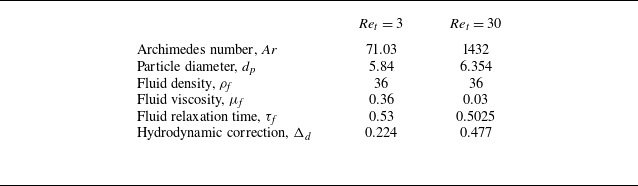
 Ret=3
 Ret=30
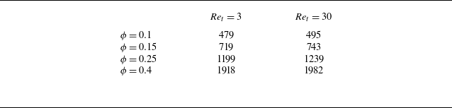
 Np
 ϕ
 Ret=3
 Ret=30

 Ret=30
 ρ∗=0.05
 e=1
 ϕ
 ϕ~
 0.6ϕ
 1.4ϕ
 ±40%

 Ret=3
 Ret=30
 e=1
 t0

 Ret=3
 Ret=30
 e=1
 Ret=3
 Ret=30
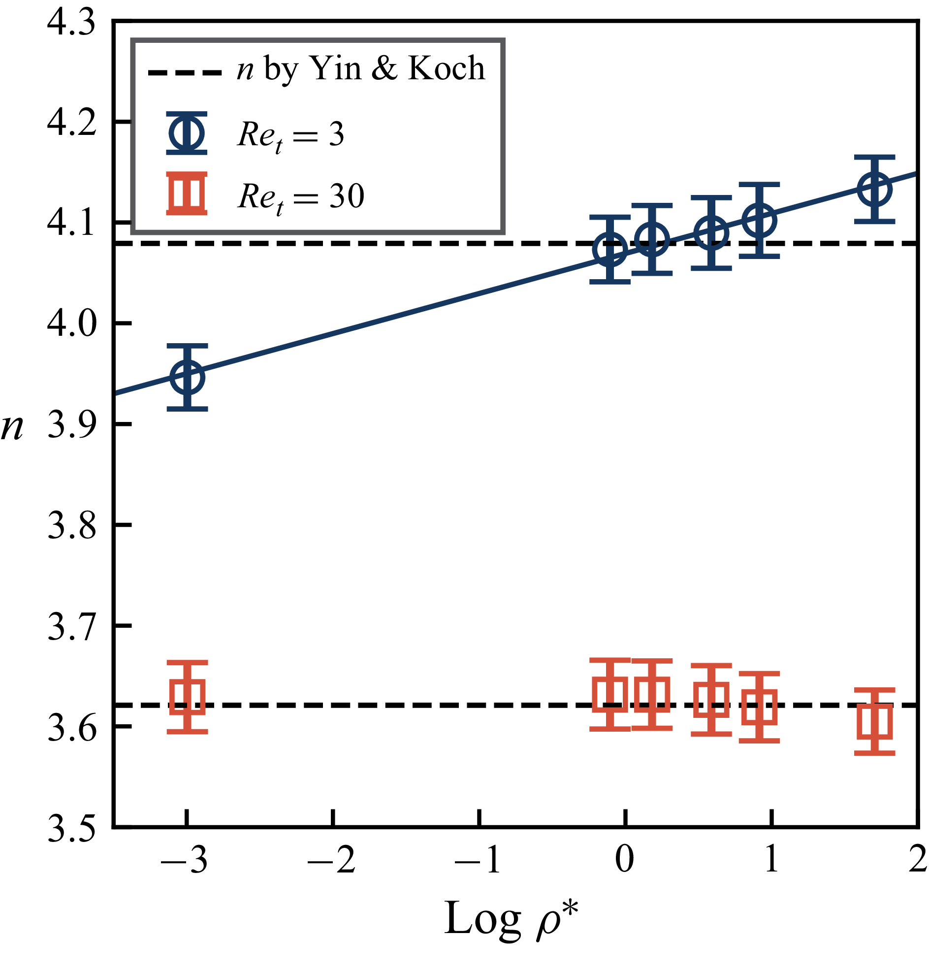
 n
 logρ∗
 e=1
 Ret=3
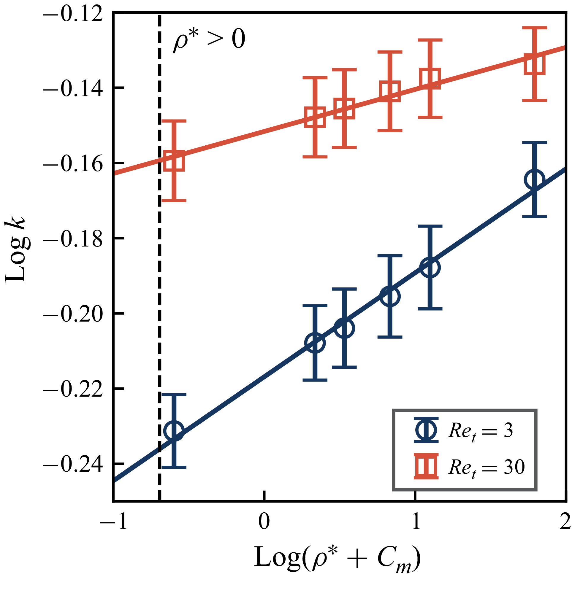
 logk
 log(ρ∗+Cm)
 e=1
 Cm=1/2
 ρ∗>0

 ReT

 ReT
 ρ∗
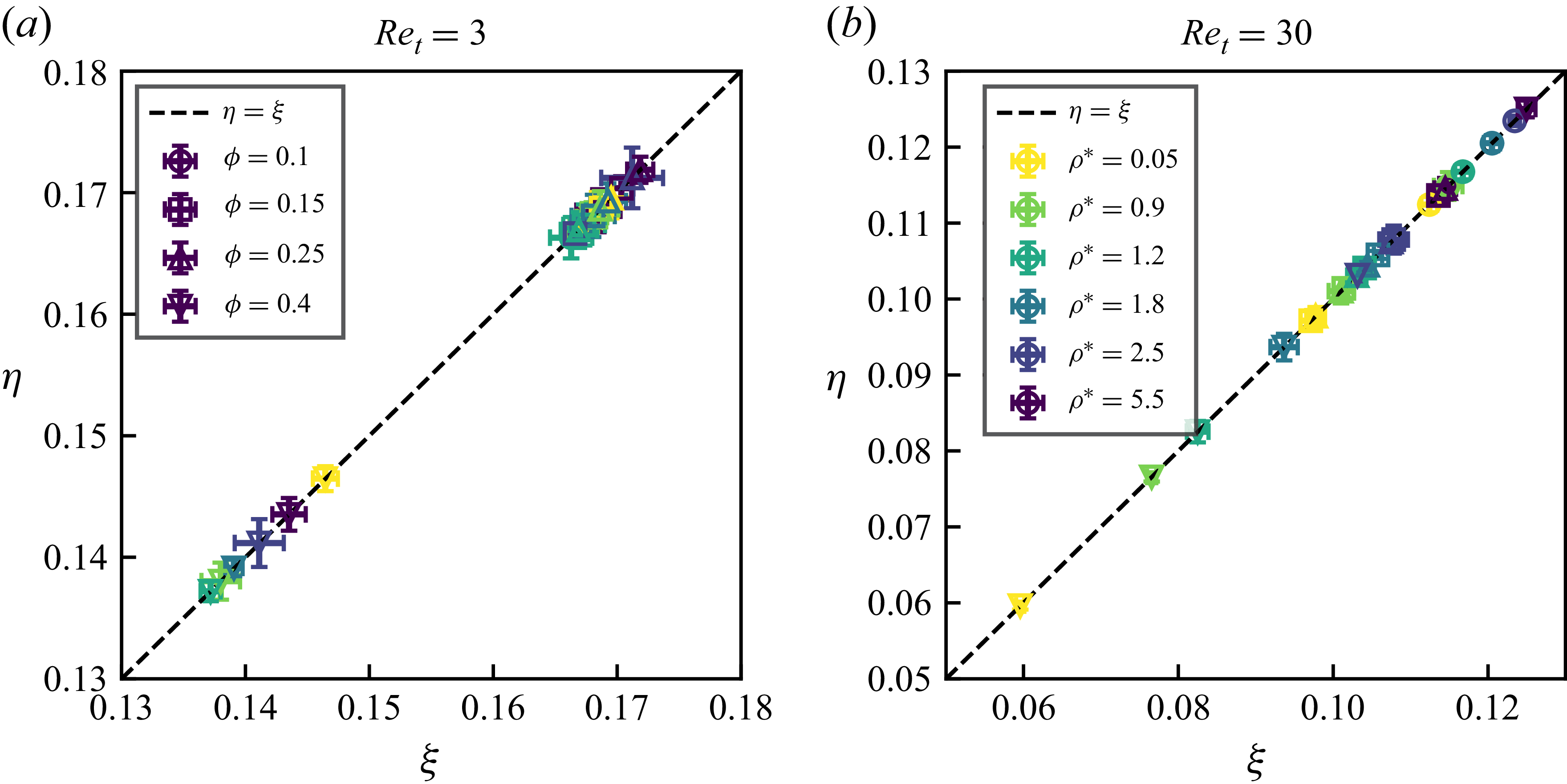
 (η,ξ)
 Ret=3
 Ret=30
 e=1
 ϕ
 ρ∗

 y
 ϕ
 Ret=3
 30
 e=0.9
 1.0
 Ret=3
 Ret=30
 e=0.9
 e=1.0
 ρ∗

 x
 y
 ϕ
 Ret=3
 30
 e=0.9
 1.0
 Ret=3
 Ret=30
 e=0.9
 e=1.0
 ρ∗

 Ret
 ϕ
 ρ∗
 y
 Ret=30
 ϕ=0.25
 e=1.0
 ρ∗=0.9
 Ryy(τ)=exp(−τ/τyyR)
 τyyR

 x
 y
 Ret=3
 Ret=30
 e=1.0

 Ret
 ϕ
 ρ∗
 Ret=30
 ϕ=0.25
 e=1.0
 ρ∗=0.9
 y

 g(r,θ)
 Ret
 ϕ
 e=1.0
 ρ∗=0.9

 g(r)
 e=1.0
 ρ∗=0.9
 Ret=3
 Ret=30

 g(r)
 Ret=30
 e=1.0
 ϕ=0.1
 ϕ=0.25
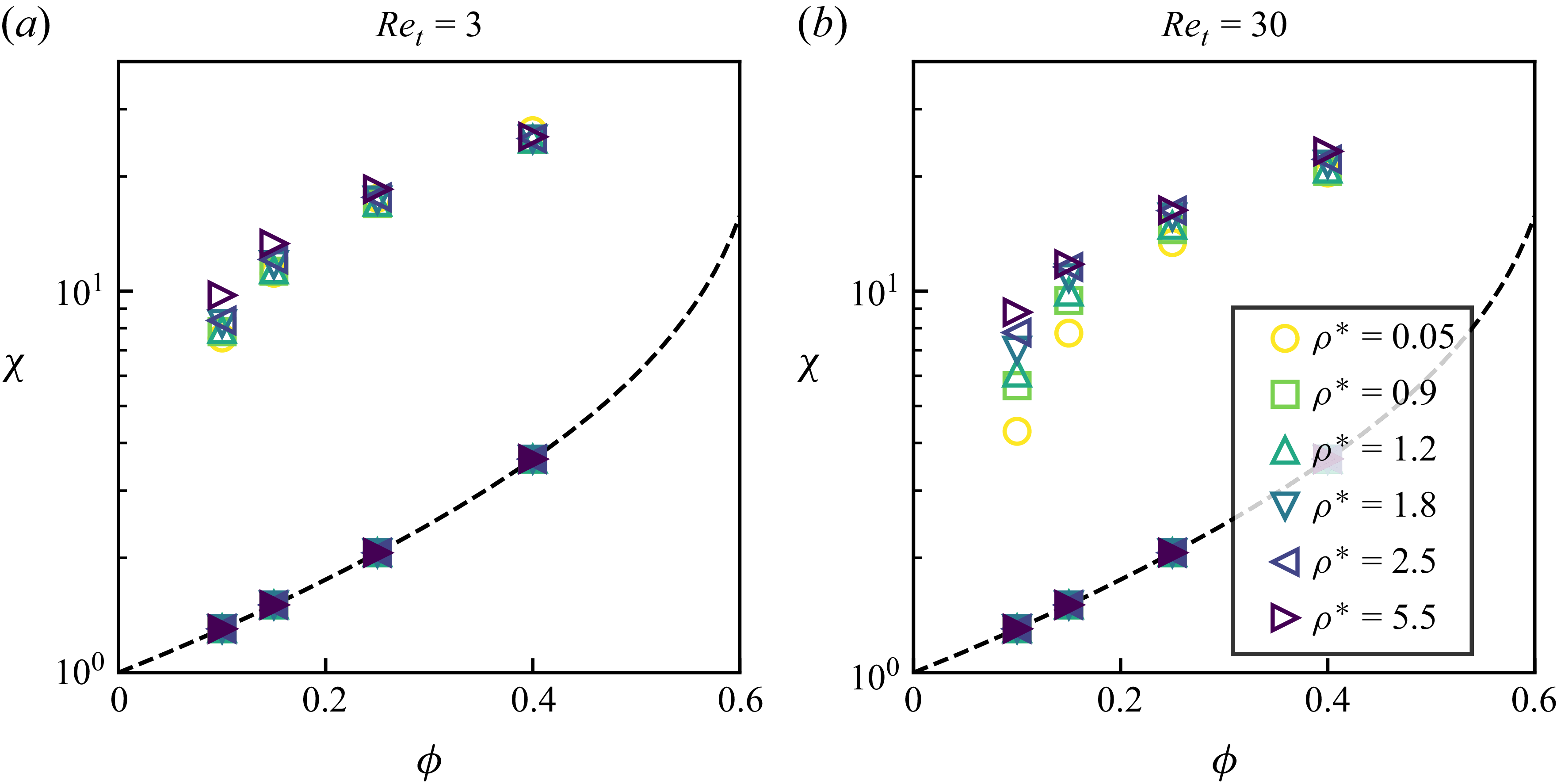
 χ
 Ret=3
 Ret=30
 εs

 Ret=3
 Ret=30
 e=1.0

 χ
 Ret=3
 Ret=30
 e=1.0

 Γc∗
 Ret=3
 Ret=30
 e=0.9

 Ret=3
 Ret=30


