



1. Introduction
Radial spreading of a liquid film after a vertical jet hits the rigid surface appears in two classic problems. They are a circular hydraulic jump on a fixed plane and a thin film flow over a rotating disk.
The statement of the first problem is the following. A vertical liquid jet falls on a horizontal disk and spreads radially, forming a thin film. At a certain distance from the fall point, the film thickness abruptly increases – one observes the hydraulic jump (Rayleigh Reference Rayleigh1914). The jump separates supercritical and subcritical flows where the gravity wave velocity is smaller and larger than the liquid velocity. A hydraulic jump is an analogue to a shock wave in the shallow-water gas-dynamics analogy framework (Landau & Lifshitz Reference Landau and Lifshitz1987). This analogy allows using the hydraulic jump for small-scale laboratory modelling of detonation (Kasimov Reference Kasimov2008), white holes (Volovik Reference Volovik2005; Jannes et al. Reference Jannes, Piquet, Maïssa, Mathis and Rousseaux2011) and accretion (Foglizzo et al. Reference Foglizzo, Masset, Guilet and Durand2012) in astrophysics.
The ideal liquid theory used by Lord Rayleigh (Reference Rayleigh1914) includes inertia and gravity and does not predict the location of the jump. The axisymmetric flow from a source has two solutions with either supercritical or subcritical flow everywhere. Taking viscosity into account in supercritical flow defines the location of the jump (Watson Reference Watson1964; Rozhdestvenskii Reference Rozhdestvenskii1979; Bohr, Dimon & Putkaradze Reference Bohr, Dimon and Putkaradze1993).
For usual laboratory experiments and applications, capillarity is negligible in the momentum equations for smooth parts of steady flows (Duchesne, Andersen & Bohr Reference Duchesne, Andersen and Bohr2019). However, the surface tension forces add a term to the momentum jump conditions (Bush & Aristoff Reference Bush and Aristoff2003) and affect the boundary conditions at the disk edge (Mohajer & Li Reference Mohajer and Li2015). Capillarity influences the stability of the hydraulic jump (Fernandez-Feria, Sanmiguel-Rojas & Benilov Reference Fernandez-Feria, Sanmiguel-Rojas and Benilov2019) and leads to the non-existence of a steady axisymmetric solution Kasimov (Reference Kasimov2008). For liquids with low surface tension (e.g. silicone oils), the capillarity is negligible. Experiments (Duchesne, Lebon & Limat Reference Duchesne, Lebon and Limat2014) and calculations (Wang & Khayat Reference Wang and Khayat2019) show that the hydraulic jump forms a flow with a specific Froude number in this case.
Bhagat et al. (Reference Bhagat, Jha, Linden and Wilson2018) and Bhagat & Linden (Reference Bhagat and Linden2020) proposed a shallow-water theory that does not involve gravity but predicts the hydraulic jumps due to surface tension. Their theoretical results fit the experimental data for liquids with high surface tension (water, water–glycerol mixtures, water with surfactants). They stated that gravity is irrelevant for the hydraulic jump formation since they observed similar values of jump radii for the experiments with water jets hitting the vertical plate, the horizontal plate from below and for the classical situation. The experimental pictures (figure 1c from Bhagat et al. (Reference Bhagat, Jha, Linden and Wilson2018)) show that, for the flow underneath the plane, there exists a short dripping ‘crown’ but not a long film after the jump, so the shallow-water approximation is not applicable. A recent letter (Bohr & Scheichl Reference Bohr and Scheichl2021) shows mathematical faults in the theory developed in Bhagat & Linden (Reference Bhagat and Linden2020).
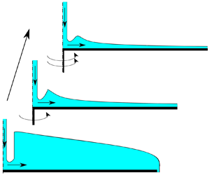
Scheme of the flow.

The second problem deals with smooth thin film flows over rotating disks. These flows appear in coating applications (Weinstein & Ruschak Reference Weinstein and Ruschak2004) and in chemical reactors (Pask, Nuyken & Cai Reference Pask, Nuyken and Cai2012). For large rotation rates, the centrifugal force is the main driving force (Espig & Hoyle Reference Espig and Hoyle1965; Charwat, Kelly & Gazley Reference Charwat, Kelly and Gazley1972). In this case, a liquid film on a rotating disk is similar to a falling film (Kapitza & Kapitza Reference Kapitza and Kapitza1949). The flow is unstable for long waves; the scale of the growing waves indicates a balance of the centrifugal force, viscosity and capillarity (Shkadov Reference Shkadov1967; Sisoev, Matar & Lawrence Reference Sisoev, Matar and Lawrence2003). The influence of gravity stabilises the flow; the Needham criterion (Needham & Merkin Reference Needham and Merkin1987) predicts that the flow is stable if the ratio of centrifugal force at the reference radius and gravity is below a specific value of the order of unity.
Interesting effects take place if the inertia, gravity and centrifugal forces have the same order. This situation corresponds to a relatively low rotation rate (Pask et al. Reference Pask, Nuyken and Cai2012). The centrifugal force adds momentum to the liquid and pushes the hydraulic jump away from the axis of rotation (Ozar, Cetegen & Faghri Reference Ozar, Cetegen and Faghri2003; Wang & Khayat Reference Wang and Khayat2018). The model considered by Wang & Khayat (Reference Wang and Khayat2018) assumes synchronous rotation of the disk and the liquid. This model predicts monotonic ‘washing’ of the jump away from the disk while the rotation rate increases. However, the momentum is transferred from the disk to the liquid by viscosity, and the Coriolis force slows down this process (Myers & Lombe Reference Myers and Lombe2006). There is an interplay between all forces that define the flow regime. Near the jet impact region, viscosity balances inertia (Watson Reference Watson1964), then gravity becomes of the same order as inertia and viscosity (Bohr et al. Reference Bohr, Dimon and Putkaradze1993). Finally, in the disk periphery, the centrifugal force and viscous friction dominate (Espig & Hoyle Reference Espig and Hoyle1965). Scheichl & Kluwick (Reference Scheichl and Kluwick2019) concentrated on the case of a relatively large rotation rate, so the flow is globally supercritical, and gravity does not dominate anywhere. The same case is simulated and studied experimentally by Wang et al. (Reference Wang, Jin, Ling, Peng, Yu and Cui2020).
Our goal is to fill the gap between the two problems mentioned above, investigating the transition from the flow over a static disk with the hydraulic jump to the continuous flow on a fast rotating disk and to study the disappearance of the jump. We consider the rotation rate range from zero to large enough values that ensure globally supercritical flow.
We extend the shallow-water theory proposed by Bohr et al. (Reference Bohr, Dimon and Putkaradze1993) for the flow over a rotating disk. We derive governing equations taking the inertia, hydrostatic pressure gradient, centrifugal and Coriolis forces into account. The surface tension influences boundary conditions but is neglected in the equations for smooth parts of the flow. We perform a qualitative analysis of the equations showing the structure of the solutions and obtain estimates for parameters corresponding to the existence of a hydraulic jump.
We derive the governing equations in § 2 and provide their qualitative analysis in § 3 followed by numerical calculation and comparison with experiments (§ 4). We summarise our results in § 5.
2. Governing equations
In this section, we state the problem. First, we describe the system, provide dimensional equations and boundary conditions. We introduce non-dimensional coordinates and parameters following Bohr et al. (Reference Bohr, Dimon and Putkaradze1993); we simplify the equations and discuss the range of validity of our assumptions. Finally, we derive the system of ordinary differential equations (ODE) for depth-averaged characteristics to be analysed further.
2.1. Dimensional equations
Consider the round jet of an incompressible fluid that falls to the centre of a horizontal rotating disk. The jet is vertical and has a constant flow rate of  $Q$. The angular velocity
 $\varOmega$ of the disk is constant. The disk radius is
 $R_f$.
In the vicinity of the disk centre, the fluid changes the direction of motion from vertical to radial. Viscous effects are negligible in this region (Watson Reference Watson1964). Further, inertia, viscous friction and gravity define the flow. We consider steady axially symmetric flow in the region where the viscous flow is fully developed.
In cylindrical coordinates (figure 1), the momentum Navier–Stokes and continuity equations for axisymmetric flow in an inertial frame are (Batchelor Reference Batchelor2000)
 $$\begin{gather} V_R\dfrac{\partial V_R}{\partial R}+V_Z\dfrac{\partial V_R}{\partial Z}-\frac{V_\varphi^2}{R}={-}\frac{1}{\rho}\dfrac{\partial P}{\partial R}+\nu\left[ \dfrac{\partial ^2V_R}{\partial Z^2}+\frac{1}{R}\dfrac{\partial }{\partial R}\left(R\dfrac{\partial V_R}{\partial R}\right)-\frac{V_R}{R^2}\right], \end{gather}$$
 $$\begin{gather}V_R\dfrac{\partial V_\varphi}{\partial R}+V_Z\dfrac{\partial V_\varphi}{\partial Z}+\frac{V_R V_\varphi}{R}=\nu\left[\dfrac{\partial ^2V_\varphi}{\partial Z^2}+\frac{1}{R}\dfrac{\partial }{\partial R}\left(R\dfrac{\partial V_\varphi}{\partial R}\right)-\frac{V_\varphi}{R^2}\right], \end{gather}$$
 $$\begin{gather}V_R\dfrac{\partial V_Z}{\partial R}+V_Z\dfrac{\partial V_Z}{\partial Z}={-}\frac{1}{\rho}\dfrac{\partial P}{\partial Z}-g+\nu\left[ \dfrac{\partial ^2V_Z}{\partial Z^2}+\frac{1}{R}\dfrac{\partial }{\partial R}\left(R\dfrac{\partial V_Z}{\partial R}\right)\right], \end{gather}$$
 $$\begin{gather}\dfrac{\partial V_R}{\partial R}+\frac{V_R}{R}+\dfrac{\partial V_Z}{\partial Z}=0, \end{gather}$$
where  $V_R(R, Z)$,
 $V_\varphi (R, Z)$,
 $V_Z(R, Z)$ are the radial, azimuthal and vertical components of the velocity,
 $P$ is pressure,
 $R$ is the coordinate along the disk radius,
 $Z$ is the coordinate along the vertical axis (
 $Z = 0$ corresponds to the disk plane),
 $\rho$ is the fluid density,
 $\nu$ is kinematic viscosity and
 $g$ is the gravitational acceleration.
At the disk surface, the no-slip boundary condition reads
 \begin{equation} V_R(R, 0) = V_Z(R, 0) = 0,\quad V_\varphi(R, 0) = \varOmega R. \end{equation}
At the free surface  $Z=H(R)$, boundary conditions state no-penetration, zero shear projections to the (
 $R,Z$) plane and azimuthal direction, action of surface tension (coefficient
 $\sigma$) and external constant pressure
 $P_0$
 $$\begin{gather} V_Z = V_R\frac{\textrm{d}H}{\textrm{d}R}, \end{gather}$$
 $$\begin{gather}\left(\dfrac{\partial V_R}{\partial Z}+\dfrac{\partial V_Z}{\partial R}\right)\left[1-\left(\frac{\textrm{d}H}{\textrm{d}R}\right)^2\right]+2\left(\dfrac{\partial V_Z}{\partial Z}-\dfrac{\partial V_R}{\partial R}\right)\frac{\textrm{d}H}{\textrm{d}R} = 0, \end{gather}$$
 $$\begin{gather}\dfrac{\partial V_\varphi}{\partial Z}- R\dfrac{\partial }{\partial R}\left(\frac{V_\varphi}{R}\right)\frac{\textrm{d}H}{\textrm{d}R} = 0, \end{gather}$$
 $$\begin{gather}P - 2\rho \nu \left[\dfrac{\partial V_Z}{\partial Z}-\left(\dfrac{\partial V_R}{\partial Z}+\dfrac{\partial V_Z}{\partial R}\right)\frac{\textrm{d}H}{\textrm{d}R}-\dfrac{\partial V_R}{\partial R}\left(\frac{\textrm{d}H}{\textrm{d}R}\right)^2 \right]= P_0 -2\sigma \kappa, \end{gather}$$
where  $\kappa$ is the surface mean curvature
 \begin{equation} 2\kappa = \dfrac{1}{R}\dfrac{\textrm{d}}{\textrm{d}R}\left(\dfrac{R\dfrac{\textrm{d}H}{\textrm{d}R}}{\sqrt{1+\left(\dfrac{\textrm{d}H}{\textrm{d}R}\right)^2 }}\right). \end{equation}
We do not consider the flow in the axis of symmetry where the jet hits the disk. We set the boundary conditions at the finite distance  $R=R_s$ (inlet) specifying the value of the film thickness
 $H_s$ and velocity distribution
 \begin{equation} V_R(R_s, Z) = V_{rs}(Z),\quad V_\varphi(R_s, Z) = V_{\varphi s}(Z). \end{equation}
The value of  $H_s$ and the function
 $V_{rs}(Z)$ define the flow rate
 $Q$:
 \begin{equation} R_s\int_0^{H_s}V_{rs}(Z)\,\textrm{d}Z =q= \frac{Q}{2{\rm \pi}}. \end{equation}
Since the Navier–Stokes equations are elliptic, they require boundary conditions for all velocity components at the edge of the disk  $R=R_f$, e.g. outflow boundary conditions (Fernandez-Feria et al. Reference Fernandez-Feria, Sanmiguel-Rojas and Benilov2019).
2.2. Scales
We introduce non-dimensional coordinates, velocities and pressure. We use different scales  $R_0$ and
 $H_0$ for radial and vertical coordinates as the film thickness and typical distances to the axis of symmetry have different orders of magnitude. For given
 $R_0$,
 $H_0$, the value of the flow rate gives the scale for the radial velocity
 $U$; the aspect ratio
 $H_0/R_0$ allows us to calculate the proper scaling for the vertical velocity. For the azimuthal velocity, we introduce the relative value: the difference between local azimuthal velocity
 $V_\varphi$ of the liquid and the azimuthal velocity
 $\varOmega R$ of the disk point right below the given one. The latter provides the scale for the relative azimuthal velocity.
The dimensional coordinates and functions are
 \begin{equation} \left.\begin{array}{c} R = R_0r_1,\quad Z = H_0z_1,\quad H=H_0h_1,\\ V_R = Uv_{r1},\quad V_\varphi = \varOmega R_0r_1(1 + v_{\varphi1}),\quad V_Z = \dfrac{UH_0}{R_0}v_{z1},\\ P=P_0+\rho g H_0 p_1. \end{array}\right\} \end{equation}
Following Bohr et al. (Reference Bohr, Dimon and Putkaradze1993), we choose scales for radial coordinate  $R_0$, radial velocity
 $U$ and the film thickness
 $H_0$ so that viscous, gravity and inertial terms are of the same order if non-dimensional velocity, radial coordinate and thickness have the order of unity
 \begin{equation} \frac{U^2}{R_0}=\frac{gH_0}{R_0}=\frac{\nu U}{H_0^2}. \end{equation}
The mass conservation law (2.12) gives the third relation for  $R_0$,
 $U$,
 $H_0$
 \begin{equation} R_0UH_0=q. \end{equation}
From (2.14), (2.15), the scale parameters are
 \begin{equation} \left.\begin{array}{c} R_0 = (q^5\nu^{{-}3}g^{{-}1})^{1/8},\\ U = (q\nu g^3)^{1/8},\\ H_0 = (q\nu g^{{-}1})^{1/4}. \end{array}\right\} \end{equation}
The non-dimensional form of the problem (2.1)–(2.11a,b) has five non-dimensional parameters: two of them are physical and express the effect of rotation and surface tension, the three others are geometrical, namely non-dimensional radii of the inlet and of the disk, and the aspect ratio
 \begin{equation} \left.\begin{array}{c} \omega_1^2=\dfrac{\varOmega^2R_0^2}{U^2}=\dfrac{\varOmega^2q}{\nu g},\quad Bo_1^{{-}1}=\dfrac{\sigma}{\rho g H_0 R_0},\\ r_{1 s}=\dfrac{R_s}{R_0},\quad r_{1 f}=\dfrac{R_f}{R_0},\quad \varepsilon=\dfrac{H_0}{R_0}. \end{array}\right\} \end{equation}
For the parameters presented in table 1, typical values of geometrical parameters are
 \begin{equation} r_{1s}\lesssim 1,\quad r_{1f}\sim 10^{2}\gg1,\quad \varepsilon\sim 10^{{-}2}\ll1. \end{equation}
The Reynolds number is
 \begin{equation} Re=\frac{UH_0}{\nu}=\varepsilon^{{-}1}=\left(\frac{q^3 g}{\nu^5}\right)^{1/8}\gg1. \end{equation}
Parameters of some hydraulic jump experiments.

The centrifugal and Coriolis forces have the same order of magnitude as inertia, viscous friction and gravity if
 \begin{equation} \omega_1^2\sim 1. \end{equation}
For the values presented in table 1,  $\omega _1=1$ corresponds to
 \begin{equation} \varOmega\sim10 \text{ rad s}^{{-}1}\approx 1.5\text{ r.p.s.}=90\text{ r.p.m}. \end{equation}
Experiments by Leshev & Peev (Reference Leshev and Peev2003), Ozar et al. (Reference Ozar, Cetegen and Faghri2003) and Wang et al. (Reference Wang, Jin, Ling, Peng, Yu and Cui2020) correspond to  $\omega _1=0.5$ to
 $8$,
 $\omega _1=10$ to
 $50$ and
 $\omega _1=3.6$ to
 $40$, respectively.
2.3. Thin-layer approximation
In most experiments, the aspect ratio  $\varepsilon \ll 1$ and the governing equations (2.1)–(2.4) contain small terms and admit simplification. The Navier–Stokes equations (2.1)–(2.4) read
 \begin{equation} \left.\begin{array}{c} v_{r1}\dfrac{\partial v_{r1}}{\partial r_1}+v_{z1}\dfrac{\partial v_{r1}}{\partial z_1} -\omega_1^2r_1\left(1 + 2v_{\varphi1} + v_{\varphi1}^2\right)\\ \qquad\qquad={-}\dfrac{\textrm{d}p_1}{\textrm{d}r_1}+\dfrac{\partial ^2v_{r1}}{\partial z_1^2}+ \varepsilon^2\left[ \dfrac{1}{r_1}\dfrac{\partial }{\partial r_1}\left(r_1\dfrac{\partial v_{r1}}{\partial r_1}\right)-\dfrac{v_{r1}}{r_1^2} \right],\\ v_{r1}\dfrac{\partial v_{\varphi1}}{\partial r_1}+v_{z1}\dfrac{\partial v_{\varphi1}}{\partial z_1}+\dfrac{2v_{r1}(1+v_{\varphi1})}{r_1}=\dfrac{\partial ^2v_{\varphi1}}{\partial z_1^2}+\varepsilon^2\left[ \dfrac{1}{r_1}\dfrac{\partial }{\partial r_1}\left(r_1\dfrac{\partial v_{\varphi 1}}{\partial r_1}\right)-\dfrac{v_{\varphi 1}}{r_1^2} \right],\\ \varepsilon^2\left[ v_{r1}\dfrac{\partial v_{z1}}{\partial r_1}+v_{z1}\dfrac{\partial v_{z1}}{\partial z_1}\right]={-}\dfrac{\partial p_1}{\partial z_1}-1+\varepsilon^2\left\{ \dfrac{\partial ^2v_{z1}}{\partial z_1^2}+\varepsilon^2\left[\dfrac{1}{r_1}\dfrac{\partial }{\partial r_1}\left(r_1\dfrac{\partial v_{z1}}{\partial r_1}\right)\right]\right\},\\ \dfrac{\partial v_{r1}}{\partial r_1}+\dfrac{v_{r1}}{r_1}+\dfrac{\partial v_{z1}}{\partial z_1}=0. \end{array}\right\} \end{equation}
The boundary conditions (2.5a,b)–(2.10) have the following form: at  $z_1=0$
 \begin{equation} v_{r1}= v_{z1}=v_{\varphi 1}= 0; \end{equation}
at  $z_1=h_1(r_1)$
 $$\begin{gather} v_{z1} = v_{r1}\frac{\textrm{d}h_1}{\textrm{d}r_1}, \end{gather}$$
 $$\begin{gather}\left( \dfrac{\partial v_{r1}}{\partial z_1}+\varepsilon^2 \dfrac{\partial v_{z1}}{\partial r_1}\right)\left[1-\varepsilon^2\left(\frac{\textrm{d}h_1}{\textrm{d}r_1}\right)^2\right]+2\varepsilon^2\left(\dfrac{\partial v_{z1}}{\partial z_1}-\dfrac{\partial v_{r1}}{\partial r_1}\right)\frac{\textrm{d}h_1}{\textrm{d}r_1}= 0, \end{gather}$$
 $$\begin{gather}\dfrac{\partial v_{\varphi 1}}{\partial z_1}-\varepsilon^2 r_1\dfrac{\partial }{\partial r_1}\left(\frac{v_{\varphi 1}}{r_1}\right)\frac{\textrm{d}h_1}{\textrm{d}r_1}= 0, \end{gather}$$
 $$\begin{gather}p_1 - 2\varepsilon^2 \left[\dfrac{\partial v_{z1}}{\partial z_1}-\left(\dfrac{\partial v_{r1}}{\partial z_1}+\varepsilon^2 \dfrac{\partial v_{z1}}{\partial r_1}\right)\frac{\textrm{d}h_1}{\textrm{d}r_1}-\dfrac{\partial v_{r1}}{\partial r_1}\left(\frac{\textrm{d}h_1}{\textrm{d}r_1}\right)^2 \right]={-}2\varepsilon Bo_1^{{-}1} \kappa_1, \end{gather}$$
the non-dimensional curvature  $\kappa _1$ is
 \begin{equation} 2\kappa_1 = \dfrac{1}{r_1}\dfrac{\textrm{d}}{\textrm{d}r_1}\left(\dfrac{r_1\dfrac{\textrm{d}h_1}{\textrm{d}r_1}}{\sqrt{1+\varepsilon^2\left(\dfrac{\textrm{d}h_1}{\textrm{d}r_1}\right)^2 }}\right). \end{equation}
Omitting small terms of the order of  $\varepsilon ^2$ and
 $\varepsilon Bo^{-1}$, we simplify the problem. The problem for pressure separates from the one for velocity and gives the hydrostatic pressure distribution
 \begin{equation} p_1 = h_1(r_1) - z_1. \end{equation}
The equations (2.22) together with (2.29) read
 \begin{equation} \left.\begin{array}{c} v_{r1}\dfrac{\partial v_{r1}}{\partial r_1}+v_{z1}\dfrac{\partial v_{r1}}{\partial z_1} -\omega_1^2r_1\left(1 + 2v_{\varphi1} + v_{\varphi1}^2\right)={-}\dfrac{\textrm{d}h_1}{\textrm{d}r_1}+\dfrac{\partial ^2v_{r1}}{\partial z_1^2},\\ v_{r1}\dfrac{\partial v_{\varphi1}}{\partial r_1}+v_{z1}\dfrac{\partial v_{\varphi1}}{\partial z_1}+\dfrac{2v_{r1}(1+v_{\varphi1})}{r_1}=\dfrac{\partial ^2v_{\varphi1}}{\partial z_1^2},\\ \dfrac{\partial v_{r1}}{\partial r_1}+\dfrac{v_{r1}}{r_1}+\dfrac{\partial v_{z1}}{\partial z_1}=0. \end{array}\right\} \end{equation}
The boundary conditions (2.23)–(2.26) transform to
 \begin{equation} \left.\begin{array}{c} v_{r1}(r_1, 0) = v_{\varphi1}(r_1, 0) = v_{z1}(r_1, 0) = 0,\\ v_{z1}(r_1, h_1)=v_{r1}(r_1, h_1)\dfrac{\textrm{d}h_1}{\textrm{d}r_1},\\ \dfrac{\partial v_{r1}(r_1, h_1)}{\partial z_1} = \dfrac{\partial v_{\varphi1}(r_1, h_1)}{\partial z_1}= 0. \end{array}\right\} \end{equation}
The derivation implies that the non-dimensional free surface slope is less or of the order of unity. Hence, the regions where this assumption does not hold, namely, the jet impact region (inlet), the hydraulic jump and the disk edge, require separate consideration.
2.4. Boundary conditions
This subsection considers the regions where the thin-layer approximation is not valid. These regions are the inlet, the hydraulic jump and the outer edge of the disk. We replace the consideration of the complex two-dimensional flow with boundary conditions.
2.4.1. Inlet conditions
The inlet boundary conditions at  $R=R_s$ (2.11a,b)–(2.12) in non-dimensional form are
 \begin{equation} \left.\begin{array}{c} v_{r1}(r_{1s}, z_1) = v_{rs}(z_1),\quad v_{\varphi1}(r_{1s}, z_1) = v_{\varphi s}(z_1),\\[8pt] \displaystyle h_1(r_{1s})=h_{1s},\quad r_{1s}\int_0^{h_{1s}}v_{rs}(z_1)\,\textrm{d}z_1 = 1,\\ v_{r s}=\dfrac{V_{r s}}{U},\quad v_{\varphi s}=\dfrac{V_{\varphi s}}{\varOmega R_s} -1. \end{array}\right\} \end{equation}
These boundary conditions match the flow in the considered domain with the one near the impact area. After the jet hits the disk, the liquid changes the direction of motion, and the viscous friction at the disk surface affects the velocity distribution. We put the boundary  $r_{1s}$ at the point where the viscous radial flow becomes fully developed. The location of this point depends on the jet Reynolds number
 $Re_{jet}=Q/(\nu a)$, where
 $a$ is the jet radius.
If  $Re_{jet}\gg 1$, the boundary layer takes some space to grow throughout the film; Watson (Reference Watson1964) estimated the location where it reaches the free surface, and a self-similar solution develops at
 \begin{equation} R_s=0.3155 a Re_{jet}^{1/3}. \end{equation}
This value corresponds to
 \begin{equation} r_{1s}=0.581\left(\frac{a^3g}{\nu^2}\right)^{2/9}Re^{{-}7/9}. \end{equation}
This solution states a film thickness of (in the present notation)
 \begin{equation} h_{1s}=1.94\left(\frac{a^3g}{\nu^2}\right)^{4/9}Re^{{-}14/9}=5.74r_{1s}^2. \end{equation}
The radial velocity distribution is
 \begin{equation} v_{rs}=v_{rs0}f_{w}(z_1),\quad v_{rs0}=\frac{1}{r_{1s}h_{1s}}, \end{equation}
where  $v_{rs0}$ is the mean velocity value, and the function
 $f_w$ is a solution of the boundary-value problem for the ODE
 \begin{equation} f_w''=cf_w^2,\quad f_w(0)=0,\quad f_w'(1)=0,\quad \int_0^1f_w(\zeta)\,\textrm{d}\zeta=1. \end{equation}
The value of  $v_{rs0}$ ensures that the velocity at the free surface equals the jet velocity for
 $r=r_{1s}$. At this location, the surface velocity starts changing.
For low values of  $Re_{jet}$ this solution is not valid as it gives
 $R_s< a$. In this case, numerical modelling of the two-dimensional flow gives the radius where the free surface becomes nearly horizontal and viscous stresses become significant throughout the film thickness. Calculations (Sisoev, Tal'drik & Shkadov Reference Sisoev, Tal'drik and Shkadov1986) show that the free surface velocity remains nearly constant while
 $R< R_s=ka$ for some constant
 $k$. The value of
 $k$ can be a fitting parameter for comparing the results of calculations with the experimental data. The velocity distribution
 $v_{rs}(z_1)$ is a smooth function with zero value at
 $z_1=0$, zero derivative at
 $z_1=h_{1s}$, unit value of the integral from
 $z_1=0$ to
 $z_1=h_{1s}$ and value of the function at
 $z_1=h_{1s}$ equal to the jet velocity. The second derivative of this function is negative everywhere due to the relaxation of the viscous stresses.
In experiments considering the flow over a rotating disk, e.g. Leshev & Peev (Reference Leshev and Peev2003), Ozar et al. (Reference Ozar, Cetegen and Faghri2003) and Wang et al. (Reference Wang, Jin, Ling, Peng, Yu and Cui2020), the jet is non-swirling. During the development of the velocity profile in the radial direction, the azimuthal velocity changes. Asymptotically, its distribution reflects the balance between viscous and Coriolis forces (Sisoev et al. Reference Sisoev, Tal'drik and Shkadov1986), but at a small or finite distance from the axis, this velocity profile is different (Myers & Lombe Reference Myers and Lombe2006). Since the viscous friction with the disk is the only source of non-zero azimuthal velocity, we take the following limitations for the function  $v_{\varphi s}$:
 \begin{equation} -1\leq v_{\varphi s}\leq0, \end{equation}
which means that the liquid cannot overtake the disk rotation and counter-rotate.
2.4.2. Jump conditions
Governing equations (2.30) express momentum and mass conservation laws assuming the free surface slope is small, and the vertical velocity is much smaller than the radial one. We replace these equations in the regions inside the computational domain where the assumption fails by integral conservation laws and treat the regions as the discontinuity surfaces.
The flow with balanced inertia and viscous friction, e.g. the self-similar flow (Watson Reference Watson1964), exhibits blow-up at a finite distance from the axis of symmetry (Bohr et al. Reference Bohr, Dimon and Putkaradze1993), the flow drops from the supercritical to subcritical flow regime, forming a hydraulic jump. A detailed description of the jump involves recirculation zones near the free surface or the disk (Bush & Aristoff Reference Bush and Aristoff2003). It requires special effort to model in the framework of the thin-layer equations (Watanabe, Putkaradze & Bohr Reference Watanabe, Putkaradze and Bohr2003). For simplification, as the transition region from supercritical to subcritical flow is usually much shorter than the reference length  $R_0$, the discontinuity is a suitable replacement of this region, similarly to the shock wave in gas dynamics.
Mass flux is continuous at the jump; the momentum flux is affected by surface tension (Bush & Aristoff Reference Bush and Aristoff2003). In the dimensional form, the jump conditions are
 \begin{align} \int_0^{H^{(1)}}V_R^{(1)}\,\textrm{d}Z&=\int_0^{H^{(2)}}V_R^{(2)}\,\textrm{d}Z, \end{align}
 \begin{align} \rho \int_0^{H^{(1)}} (V_R^{(1)})^2 \,\textrm{d}Z + \int_0^{H^{(1)}} P^{(1)} \,\textrm{d}Z &=\rho \int_0^{H^{(2)}}(V_R^{(2)})^2 \,\textrm{d}Z + \int_0^{H^{(2)}} P^{(2)} \,\textrm{d}Z\nonumber\\ &\quad +\sigma \frac{H^{(2)}-H^{(1)}}{R_j}+\int_{H^{(1)}}^{H^{(2)}}P_0\,\textrm{d}Z. \end{align}
Here, the superscripts ‘(1)’ and ‘(2)’ denote the magnitudes of quantities before and after the jump. Transferring to non-dimensional variables (2.13) gives the following conditions:
 \begin{align} \left.\begin{array}{c} \displaystyle r_j\int_0^{h_1^{(1)}}v_{r1}^{(1)}(z_1)\,\textrm{d}z_1 =r_j\int_0^{h_1^{(2)}}v_{r1}^{(2)}(z_1)\,\textrm{d}z_1=1,\\ \displaystyle \int_0^{{h_1}^{(1)}} (v_{r1}^{(1)})^2\,\textrm{d}z_1 + \dfrac{1}{2}(h_1^{(1)})^2 = \int_0^{{h_1}^{(2)}} (v_{r1}^{(2)})^2\,\textrm{d}z_1 + \dfrac{1}{2}(h^{(2)})^2 +Bo_1^{{-}1}\dfrac{h^{(2)}-h^{(1)}}{r_j}. \end{array}\right\} \end{align}
For rotating flows, the circular hydraulic jump is an oblique shock and the shock condition for the tangential velocity component (conservation of the angular momentum) completes the Rayleigh conditions (2.41):
 \begin{equation} r_j\int_0^{h_1^{(1)}}v_{r1}^{(1)}(z_1)v_{\varphi 1}^{(1)}(z_1)\,\textrm{d}z_1 =r_j\int_0^{h_1^{(2)}}v_{r1}^{(2)}(z_1)v_{\varphi 1}^{(2)}(z_1)\,\textrm{d}z_1. \end{equation}
Unlike the problem of a rotating curvilinear hydraulic jump considered by Ivanova & Gavrilyuk (Reference Ivanova and Gavrilyuk2019), we consider axially symmetric flows and the direction of the jump is known a priori.
2.4.3. Outlet conditions
Parabolic partial differential equations, e.g. boundary layer equations, do not require boundary conditions at large values of the longitudinal coordinate and can be solved by a downstream marching procedure (Anderson Reference Anderson1995). The considered thin-layer equations (2.30) contain a hydrostatic pressure gradient term on the right-hand side. The solution depends on the downstream conditions if the radial velocity  $v_{r1}$ is less than the gravitational wave velocity. To obtain a unique solution, we set a downstream boundary condition at some point after the jump.
Watson (Reference Watson1964) did not consider the flow after the jump and set the film thickness after the jump  $h_{1}^{(2)}$. With the self-similar solution before the jump and the jump conditions, this value fixes a unique solution and determines the jump location.
Bohr et al. (Reference Bohr, Dimon and Putkaradze1993) and Watanabe et al. (Reference Watanabe, Putkaradze and Bohr2003) showed that a solution for the flow after the jump has a singular point, where the free surface has a vertical tangent, and demand that the singularity is located at the disk edge. Kasimov (Reference Kasimov2008) extended the computational domain beyond the disk edge, attaching a step-down topography and keeping the thin-layer approximation valid. Flowing over the step-down, the liquid transfers from the subcritical to the supercritical regime. A unique solution satisfies the continuity condition during this transition. Duchesne et al. (Reference Duchesne, Lebon and Limat2014) used a general solution in the subcritical zone, which neglects the effect of inertia and assumes a parabolic velocity profile. This solution has one arbitrary constant fixed by setting the film thickness at the disk edge. In experiments, the film thickness at the disk edge is specified explicitly by a rim (Ellegaard et al. Reference Ellegaard, Hansen, Haaning, Hansen, Marcussen, Bohr, Hansen and Watanabe1998; Bush, Aristoff & Hosoi Reference Bush, Aristoff and Hosoi2006; Rojas et al. Reference Rojas, Argentina and Tirapegui2013) or defined by capillarity.
For liquids with a high value of the surface tension coefficient, the film thickness at the disk edge depends on the surface tension (Mohajer & Li Reference Mohajer and Li2015). Neglecting inertia and viscous stresses for the flow near the disk edge, we obtain that the balance of gravity and surface tension defines the free surface shape. The Young–Laplace equation specifies this (Landau & Lifshitz Reference Landau and Lifshitz1987). The film thickness is of the order of the capillary length
 \begin{equation} H(R_f)=b_1\sqrt{\frac{\sigma}{\rho g}}, \end{equation}
where  $b_1$ is constant dependent on the wetting properties of the disk edge. The maximal value of
 $b_1$ is
 $\sqrt {2}$ (Landau & Lifshitz Reference Landau and Lifshitz1987). In non-dimensional form we have
 \begin{equation} h_1(r_{1f})=b_1\sqrt{\frac{Bo_1^{{-}1}}{\varepsilon}}. \end{equation}
The solution neglecting inertia in the subcritical zone (Bohr et al. Reference Bohr, Dimon and Putkaradze1993) gives nearly constant film thickness after the jump for  $h_1(r_{1f})\gg 1$. The same outlet boundary condition describes the propagation of the liquid front over a non-wetted surface (Askarizadeh et al. Reference Askarizadeh, Ahmadikia, Ehrenpreis, Kneer, Pishevar and Rohlfs2019).
For the film on a rotating disk, the momentum flux at the disk edge is significant as the centrifugal force keeps the liquid moving. Generally, a complete numerical simulation involving jet formation at the disk edge is required (Li, Sisoev & Shikhmurzaev Reference Li, Sisoev and Shikhmurzaev2019). Simple boundary conditions such as infinite slope or a fixed thickness give the limit cases for the qualitative analysis of the flow.
2.5. Range of the model applicability
During the derivation of the governing equations (2.30) and boundary conditions at the free surface (2.31), we neglected the terms of the order of  $\varepsilon ^2$ and
 $\varepsilon Bo_1^{-1}$. The jump conditions (2.41) and the outlet conditions (2.44) involve
 $Bo_1^{-1}$,
 $Bo_1^{-1}/\varepsilon$. If at least one of these numbers is small, the model can be further simplified. In particular, small values of both of these numbers means a negligible effect of the surface tension.
Both non-dimensional parameters  $Bo_1^{-1}$ and
 $\varepsilon$ involve flow rate
 $q$. To separate the effect of surface tension and inertia we introduce a new set of non-dimensional values: the flow independent Kapitza number
 $\varGamma$ and the surface tension independent Reynolds number as
 \begin{equation} \varGamma=\frac{\sigma}{\rho g^{1/3} \nu^{4/3}},\quad Re=\left(\frac{q^3 g}{\nu^5}\right)^{1/8}. \end{equation}
Since the surface tension coefficients and densities for all liquids used in experiments (water, water with surfactants, water–glycerol mixtures, silicone oils) have the same order of magnitude (from  $20\times 10^{-3}$ to
 $72\times 10^{-3}$ N m
 $^{-1}$, from 980 to 1260 kg m
 $^{-3}$), the value of the Kapitza number is mainly affected by the viscosity.
The non-dimensional numbers of interest are
 \begin{equation} \varepsilon^2=Re^{{-}2}, \ \ Bo_1^{{-}1}=\varGamma Re^{{-}7/3}, \ \ \varepsilon Bo_1^{{-}1}=\varGamma Re^{{-}10/3},\ \ \frac{Bo_1^{{-}1}}{\varepsilon}=\varGamma Re^{{-}4/3}. \end{equation}
Figure 2 shows the ( $Re,\ \varGamma$) plane and presents the areas where assumptions for the equations (2.30) and free surface boundary conditions (2.31) hold at the level of 10 % and 1 % accuracy assuming all functions and their derivatives are of the order of unity. We also plotted reference values of the capillary term at the jump (
 $Bo_1^{-1}$) and at the disk edge (
 $Bo_1^{-1}/\varepsilon$). We put the values of the parameters from the experiments and simulations by Bhagat et al. (Reference Bhagat, Jha, Linden and Wilson2018), Bohr et al. (Reference Bohr, Dimon and Putkaradze1993), Choo & Kim (Reference Choo and Kim2016), Duchesne et al. (Reference Duchesne, Lebon and Limat2014), Fernandez-Feria et al. (Reference Fernandez-Feria, Sanmiguel-Rojas and Benilov2019), Hansen et al. (Reference Hansen, Hørlück, Zauner, Dimon, Ellegaard and Creagh1997) and Mohajer & Li (Reference Mohajer and Li2015). Microgravity experiments (Avedisian & Zhao Reference Avedisian and Zhao2000; Phillips et al. Reference Phillips, Kuhlman, Mohebbi, Calandrelli and Gray2008) correspond to the upper-left corner of the diagram (figure 2) and cannot be described by the presented model. The majority of tests (except some experiments by Hansen et al. (Reference Hansen, Hørlück, Zauner, Dimon, Ellegaard and Creagh1997) and Duchesne et al. (Reference Duchesne, Lebon and Limat2014) with highly viscous oils) lie in the thin-layer equations’ range of applicability. The capillarity is significant for the outlet boundary conditions for most cases, except the tests with highly viscous silicone oils by Duchesne et al. (Reference Duchesne, Lebon and Limat2014) and those with a water–glycerol 10/90 mixture by Bhagat et al. (Reference Bhagat, Jha, Linden and Wilson2018) (points below the lowest blue dotted line in figure 2). For water and water with surfactant experiments at the lower part of the Reynolds number range, the capillarity dominates at the outer boundary. The surface tension term in the jump conditions is significant for water and water with surfactant experiments but is negligible if water–glycerol mixtures or oils are used. The sink of the momentum flux due to gravity at the hydraulic jump is significant for all the analysed experiments.
Parameters of some experiments and simulations and range of the model applicability. Light and dark shades show areas when the omitted terms are less than 10 % and 1 %, respectively. Blue dotted and red dashed lines indicate values of the capillary terms at the disk edge and the jump. Symbols show the ranges of parameters in the cited experiments and simulations.

2.6. Equations for mean values
Following the general approach for thin film dynamics (Kalliadasis et al. Reference Kalliadasis, Ruyer-Quil, Scheid and Velarde2011), we average the equation across the film. This procedure results in an ODE system for the film thickness and mean values of the velocity components. The obtained system captures the main features of the flow dynamics and skips less important details. The averaging is consistent with the integral jump conditions. To close the equations for mean values, one has to specify the shape of the velocity profiles. In this subsection, we describe the averaging procedure, discuss the system's closure and obtain the equations for mean values to perform qualitative analysis and numerical simulations.
2.6.1. Averaging the equations
We use the von Kármán–Polhausen method (Schlichting & Gersten Reference Schlichting and Gersten2016) assuming the profiles of radial and azimuthal velocities are similar in any cross-section
 \begin{equation} v_{r 1}(r_1, z_1)=u_1(r_1)f_u\left(\frac{z_1}{h_1(r_1)}\right),\quad v_{\varphi 1}(r_1, z_1)=v_1(r_1)f_v\left(\frac{z_1}{h_1(r_1)}\right), \end{equation}
where  $f_u$ and
 $f_v$ satisfy boundary conditions (2.31) and have the unit mean values
 \begin{equation} \left.\begin{array}{c} f_u(0) = f_v(0) = 0,\\ f_u'(1) = f_v'(1) = 0,\\ \displaystyle \int_0^1 f_u(\zeta)\,\textrm{d}\zeta =1,\quad \int_0^1 f_v(\zeta) \,\textrm{d}\zeta = 1. \end{array}\right\} \end{equation}
The inlet boundary condition (2.12) and the mass conservation law give
 \begin{equation} u_1r_1h_1 = 1. \end{equation}
The von Kármán–Polhausen method is a basis of the integral boundary layer (IBL) approach (Shkadov Reference Shkadov1967) which shows strong predictive power for nonlinear waves in falling films (Kalliadasis et al. Reference Kalliadasis, Ruyer-Quil, Scheid and Velarde2011). It is a particular case of Galerkin method application with one basic function (Shkadov Reference Shkadov1967). The calculations with a large number of basic functions in the framework of the full Navier–Stokes equations for the falling film (Trifonov Reference Trifonov2014) and thin-layer equations for the flow on the static (Fernandez-Feria et al. Reference Fernandez-Feria, Sanmiguel-Rojas and Benilov2019) or fast rotating (Sisoev et al. Reference Sisoev, Tal'drik and Shkadov1986; Mogilevskii & Shkadov Reference Mogilevskii and Shkadov2009) disk show that the contribution of the first basic function is dominant apart from the regions where the free surface profile sharply changes. Bohr et al. (Reference Bohr, Dimon and Putkaradze1993) used the IBL approach for the description of the hydraulic jump. Equations obtained by this approach describe nonlinear (Sisoev et al. Reference Sisoev, Matar and Lawrence2003) and stationary spiral (Sisoev, Goldgof & Korzhova Reference Sisoev, Goldgof and Korzhova2010) waves on a rotating disk. More complicated methods involving shape factors (Watanabe et al. Reference Watanabe, Putkaradze and Bohr2003) for velocity profiles and equations for energy transport (Ivanova & Gavrilyuk Reference Ivanova and Gavrilyuk2019) allow us to study the hydraulic jump structure and other details of the flow but make the analysis much more intricate.
Integration of the momentum equations (2.30) across the film taking into account boundary conditions (2.31) and (2.49) gives
 \begin{equation} \left.\begin{array}{c} C_1u_1\dfrac{\textrm{d}u_1}{\textrm{d}r_1}-\omega_1^2r_1(1+2v_1+C_5v_1^2)={-}\dfrac{\textrm{d}h_1}{\textrm{d}r_1}-C_2\dfrac{u_1}{h_1^2},\\ \dfrac{\textrm{d}v_1}{\textrm{d}r_1}+\dfrac{2}{C_3 r_1}+2\dfrac{v_1}{r_1}={-}\dfrac{C_4}{C_3}{v_1}u_1r_1^2, \\ u_1r_1h_1 = 1,\\ \displaystyle C_1=\int_0^1f_u^2(\zeta)\,\textrm{d}\zeta,\quad C_2=f_u'(0),\\ \displaystyle C_3 = \int_0^1 f_u(\zeta)f_v(\zeta) \,\textrm{d}\zeta, \quad C_4= f_v'(0),\quad C_5=\int_0^1f_v^2(\zeta)\,\textrm{d}\zeta. \end{array}\right\} \end{equation}
The boundary conditions at  $r_1=r_{1 s}$ give the values of
 $u_1$ and
 $v_1$ in this point
 \begin{equation} \left.\begin{array}{c} h_1(r_{1 s})=h_{1 s},\quad u_1(r_{1 s})=u_{1 s},\quad v_1(r_{1 s})=v_{1 s},\\ \displaystyle u_{1 s}=\dfrac{1}{h_{1 s}}\int_0^{h_{1 s}}v_{r s}(z_1)\,\textrm{d}z_1,\\ \displaystyle v_{1 s}=\dfrac{1}{h_{1 s}}\int_0^{h_{1 s}}v_{\varphi s}(z_1)\,\textrm{d}z_1. \end{array}\right\} \end{equation}
2.6.2. Rescaling
Following Bohr et al. (Reference Bohr, Dimon and Putkaradze1993), to simplify the equations (2.50), we rescale the magnitudes for velocities and the film thickness to make the coefficients in the first equation equal to unity:
 \begin{equation} u_1 = \alpha u,\quad r_1 = \beta r, \quad h_1 = \gamma h,\quad v_1 = \delta v. \end{equation}
Substituting (2.52a–d) in (2.50), we get
 \begin{equation} \left.\begin{array}{c} \dfrac{C_1\alpha^2}{\beta} u\dfrac{\textrm{d}u}{\textrm{d}r}-\beta \omega_1^2r(1+2\delta v+C_5\delta^2v^2)={-}\dfrac{\gamma}{\beta}\dfrac{\textrm{d}h}{\textrm{d}r}-\dfrac{C_2 \alpha}{\gamma^2} \dfrac{u}{h^2},\\ \dfrac{\delta}{\beta} \dfrac{\textrm{d}v}{\textrm{d}r}+\dfrac{2}{C_3\beta r}+2\dfrac{\delta}{ \beta}\dfrac{v}{r}={-}\dfrac{C_4}{C_3}\alpha^2\beta^2\delta {v}ur^2,\\ \alpha \beta \gamma u r h=1. \end{array}\right\} \end{equation}
We choose the coefficients  $\alpha , \beta , \gamma , \delta$ to have as many unit coefficients in the system (2.53) as possible:
 \begin{equation} C_1\frac{\alpha^2}{\beta}=\frac{\gamma}{\beta},\quad C_1\frac{\alpha^2}{\beta}=C_2\frac{\alpha}{\gamma^{2}},\quad \frac{\delta}{\beta}=\frac{2}{C_3\beta},\quad \alpha\beta\gamma=1. \end{equation}
Equation (2.54a–d) gives the expressions for  $\alpha , \beta , \gamma , \delta$ via
 $C_i$,
 $i = 1\dots 5$:
 \begin{equation} \alpha=C_1^{{-}1/2}C_2^{1/8},\quad \beta=C_1^{1/2}C_2^{{-}3/8},\quad \gamma=C_2^{1/4},\quad \delta=2C_3^{{-}1}. \end{equation}
The system of equations (2.53) has the following form (primes denote derivative by  $r$):
 \begin{equation} \left.\begin{array}{c} u u'-\omega^2r(1+B_1v+B_2v^2)={-}h'-\dfrac{u}{h^2},\\ v'+\dfrac{1}{r}+\dfrac{2v}{r}={-}Avur^2,\\ uhr=1,\\ \omega^2=W^2\omega_1^2,\quad W^2=\dfrac{\beta^2}{\gamma}=\omega_1^2\dfrac{C_1}{C_2},\\ A=\dfrac{C_4 \alpha\beta^3}{ C_3 }=\dfrac{C_4 C_1}{C_3C_2},\quad B_1 = \dfrac{4}{C_3},\quad B_2 = \dfrac{4C_5}{C_3^2}. \end{array}\right\} \end{equation}
The values of the boundaries of the computational domain  $r_{1 s}$,
 $r_{1 f}$ and functions in the former point
 $u_{1 s}$ and
 $v_{1 s}$ transform into
 $r_s$,
 $r_f$,
 $u_s$,
 $v_s$ according to (2.52a–d), respectively. The jump conditions (2.41 and (2.42) for the mean values give
 \begin{equation} \left.\begin{array}{c} u^{(1)}h^{(1)}r_j =u^{(2)}h^{(2)}r_j=1,\\ (u^{(1)})^2h^{(1)} + \dfrac{1}{2}(h^{(1)})^2 = (u^{(2)})^2h^{(2)} + \dfrac{1}{2}(h^{(2)})^2 +{Bo}^{{-}1}\dfrac{h^{(2)}-h^{(1)}}{r_j},\\ v^{(1)}=v^{(2)},\\ Bo^{{-}1}=Bo_1^{{-}1}\dfrac{C_2^{1/8}}{C_1^{1/2}}. \end{array}\right\} \end{equation}
For a static disk ( $\omega =0$), the first equation of (2.56) and the first two jump conditions (2.57) coincide with those obtained by Bohr et al. (Reference Bohr, Dimon and Putkaradze1993), and the other equation and jump condition have no physical meaning.
Eliminating  $h$ from (2.56) we obtain
 $$\begin{gather} u u'-\omega^2r(1+B_1v+B_2v^2)=\frac{1}{u^2r} u'+\frac{1}{ur^2}-u^3r^2, \end{gather}$$
 $$\begin{gather}v' +2\frac{v}{r}+\frac{1}{r}={-}Auvr^2. \end{gather}$$
The boundary conditions for the system (2.58)–(2.59) are
 \begin{equation} u(r_s) = u_s,\quad v(r_s) = v_s. \end{equation}
Bohr et al. (Reference Bohr, Dimon and Putkaradze1993) proposed an equivalent form of (2.58) for  $\omega =0$ introducing a new independent variable on the integral curve. This allows numerical calculation near the fixed point (
 $r=1$,
 $u=1$). We use the same variable transformation and obtain
 \begin{equation} \left.\begin{array}{c} \displaystyle{\dfrac{\textrm{d}r}{\textrm{d}s}=u^3r^2-r,}\\ \displaystyle{\dfrac{\textrm{d}u}{\textrm{d}s}=u-u^5r^4+\omega^2u^2r^3(1+B_1v+B_2v^2),}\\ \displaystyle{\dfrac{\textrm{d}v}{\textrm{d}s} ={-}(u^3r-1)(1+2v+Avur^3).} \end{array}\right\} \end{equation}
The first equation is the definition of the new variable  $s$. The boundary conditions now are
 \begin{equation} s=0:\quad r = r_s,\ u = u_{s},\ v= v_{s}. \end{equation}
The solutions for the problem (2.58)–(2.60a,b) correspond to the solutions of (2.61)–(2.62); the latter system of equations simplifies the analysis.
2.6.3. Polynomial velocity profiles
To obtain the specific values of the coefficients  $W^2$,
 $A$,
 $B_1$,
 $B_2$,
 $C_i$,
 $i = 1\ldots 5$, we set the velocity profiles assuming that the viscous stresses in the radial direction balance an independent of
 $z_1$ force (centrifugal force, hydrostatic pressure gradient or the mean value of the inertial term) and the viscous stresses in the azimuthal direction balance the Coriolis force
 \begin{equation} \frac{\textrm{d}^2f_u}{\textrm{d}z_1^2}=\mathrm{const.},\quad \frac{\textrm{d}^2f_v}{\textrm{d}z_1^2}\sim f_u. \end{equation}
Together with boundary and normalisation conditions (2.48), this gives
 \begin{equation} f_{u}(\zeta)=\frac32 (2\zeta-\zeta^2),\quad f_{v}={-}\frac{5}{16} (4\zeta^3-\zeta^4-8\zeta),\quad \zeta=\frac{z}{h}. \end{equation}
These velocity profiles (2.64a–c) with
 \begin{equation} u=\omega^{2/3}r^{{-}1/3},\quad v={-}\frac{1}{A}\omega^{{-}2/3}r^{{-}8/3},\quad h=\omega^{{-}2/3}r^{{-}2/3} \end{equation}
are the asymptotic solution of the thin-layer equations (2.30)–(2.31) at  $r\to \infty$. Higher terms of the asymptotic are given in Shkadov (Reference Shkadov1973). The solution (2.65a–c) provides the analogy between the falling film and the film on a rotating disk and is referred to as the Nusselt solution. Shkadov (Reference Shkadov1967), Bohr et al. (Reference Bohr, Dimon and Putkaradze1993) and Sisoev et al. (Reference Sisoev, Matar and Lawrence2003) used these functions for finite thickness film modelling.
The use of functions  $f_u$,
 $f_v$ different from (2.64a–c), e.g. self-similar solution
 $f_u=f_w$ given by (2.37a–d) and
 $f_v$ defined by (2.63a,b) (Bush & Aristoff Reference Bush and Aristoff2003; Askarizadeh et al. Reference Askarizadeh, Ahmadikia, Ehrenpreis, Kneer, Pishevar and Rohlfs2019) changes the coefficients of (2.56), but not the structure of equations. Table 2 gives the values of the coefficients for the profiles (2.64a–c) and self-similar profile (2.37a–d) referred to as polynomial and self-similar. Figure 3 shows these velocity profiles. Despite the relatively large discrepancy in
 $C_2$ and
 $W^2$, the equations (2.56) contain only
 $A$,
 $B_1$,
 $B_2$ which weakly depend on the profile and do not affect qualitative properties of the system. Further, we use polynomial velocity profiles for the calculations.
Profiles of radial (a) and azimuthal (b) velocity.

Coefficients for different velocity profiles.

3. Qualitative analysis
In this section, we analyse fixed points of (2.61). This analysis predicts the existence or absence of a hydraulic jump and gives an estimation of its location. We recall results for the static disk (Bohr et al. Reference Bohr, Dimon and Putkaradze1993) and study the transformation of the system properties while  $\omega \neq 0$.
3.1. General properties
Consider  $\omega =0$. The system (2.61) has the form (Bohr et al. Reference Bohr, Dimon and Putkaradze1993)
 \begin{equation} \left.\begin{array}{c} \displaystyle\dfrac{\textrm{d}r}{\textrm{d}s}=u^3r^2-r,\\[8pt] \displaystyle\dfrac{\textrm{d}u}{\textrm{d}s}=u-u^5r^4. \end{array}\right\} \end{equation}
At the line
 \begin{equation} u^3r=1, \end{equation}
we have  $\textrm {d}r/\textrm {d}s=0$ and thus
 $\textrm {d}u/\textrm {d}r=\infty$. This line at the
 $(r,u)$ plane separates supercritical (above the line) and subcritical (below the line) flow regimes as the local Froude number indicates the ratio of the velocity and the gravity wave speed. It equals
 \begin{equation} Fr=\frac{u^2}{h}=u^3r. \end{equation}
The point  $(r, u) = (1, 1)$ is a fixed point, its type is a stable focus. Approaching this point, all phase trajectories are ‘spiralling’ and there are multiple values of
 $u$ for a given value of
 $r$ close to 1.
Bohr et al. (Reference Bohr, Dimon and Putkaradze1993) proved that for any phase trajectory  $u$ is uniquely defined for
 $r$ from a finite segment only. For boundary conditions and parameters corresponding to experiments (table 1), the trajectory going through the point (
 $r_s,\ u_s$) does not reach
 $r_f$ and no continuous solution exists. To obtain the overall solution at the interval
 $(r_s,r_f)$, one considers two parts of the solution separately. The inner solution describes the supercritical flow at
 $r_s\leq r< r_j$, the outer one is defined at
 $r_j< r\leq r_f$ and corresponds to subcritical flow. Here,
 $r_j$ is the a priori unknown location of the hydraulic jump.
The outer solution requires boundary conditions at  $r_f$. Bohr et al. (Reference Bohr, Dimon and Putkaradze1993) and Watanabe et al. (Reference Watanabe, Putkaradze and Bohr2003) stated that the outer solution has a singularity (
 $\textrm {d}u/\textrm {d}r=\infty$) at the disk edge, Kasimov (Reference Kasimov2008) considered the flow beyond the disk edge adding a step-down topography and found a continuous solution at the step-down. Duchesne et al. (Reference Duchesne, Lebon and Limat2014) fixed a film thickness at
 $r_f$. All these boundary conditions lead to close prediction of the jump locations, provided
 $r_f$ is large enough.
To find the jump location  $r_j$, we integrate (3.1) from
 $r_s$ towards larger
 $r$ and from
 $r_f$ towards smaller values. The integration stops at the point when
 ${\rm d}r/{\rm d}s$ changes sign. We find the point
 $r_j$ in the common domain of definition for inner and outer solutions where Rayleigh jump conditions (2.57) hold.
For  $\omega >0$, we introduce the radial Froude number
 \begin{equation} Fr_r = \frac{u^2}{h}=u^3r. \end{equation}
Further, we will refer to the region with  $Fr_r > 1$ as supercritical and
 $Fr_r < 1$ as subcritical, although the total Froude number can be larger than one.
Due to the asymptotic solution (2.65a–c), the radial Froude number at infinity is
 \begin{equation} Fr_r=\omega^2. \end{equation}
For  $\omega ^2<1$, the flow is subcritical at infinity. If the flow is supercritical at
 $r_s$, it must change its type from supercritical to subcritical at least once. Due to continuity, one expects hydraulic jump formation for the transition from supercritical to the subcritical regime, at least for small
 $\omega$.
3.2. Estimation of azimuthal velocity
Purely radial spreading is impossible for the flow over the rotating disk due to the Coriolis force:  $v\equiv 0$ does not satisfy the angular momentum equation (2.59). The relative azimuthal velocity
 $v$ defines the local centrifugal force, the last term in the left-hand side of the radial momentum equation (2.58). This term makes the main difference between flows over the static and rotating disks, and thus the qualitative analysis requires estimations for
 $v$.
3.2.1. Global estimation
The liquid gets azimuthal momentum by viscous friction. Hence, the relative azimuthal velocity  $v$ has limitations. On the one hand, the disk pulls the liquid, and the latter cannot overtake the former. On the other hand, the liquid must follow the disk, so the liquid azimuthal velocity has the same direction. The inequality (2.38) holds for the entire domain. Taking into account scaling (2.55a–d), we obtain the global estimation
 \begin{equation} -\frac{68}{175}=v_m\leq v<0\quad \forall r. \end{equation}
3.2.2. Supercritical region
The equation for angular momentum (2.59) allows us to enhance the lower estimation in the supercritical region  $r_s< r< r_j$. There,
 $Fr_r=u^3r\geq 1$ then
 \begin{equation} \frac{\textrm{d}v}{\textrm{d}r} ={-}2\frac{v}{r}-\frac{1}{r}-Avur^2 \geq{-}2\frac{v}{r}-\frac{1}{r}-Avr^{5/3}. \end{equation}
Consider the function  $\tilde {v}$ such that its derivative is the right-hand side of (3.7), and its value at
 $r=r_s$ is the minimum possible velocity
 $v=v_m$. The equation for
 $\tilde {v}$ is
 \begin{equation} r\frac{\textrm{d}\tilde{v}}{\textrm{d}r} + (2+Ar^{8/3})\tilde{v} ={-}1, \quad \tilde{v}(r_i)=v_m, \end{equation}
which is a linear heterogeneous equation with the solution
 \begin{align} \tilde{v}&=v_m\left(\frac{r_s}{r}\right)^2\exp\left[-\frac{3A}{8}(r^{8/3}-r_s^{8/3}) \right]\nonumber\\ &\quad -\exp\left(-\frac{3A}{8}r^{2/3}\right)\int_{r_s}^{r}\xi\exp\left(\frac{3A}{8}\xi^{8/3}\right)\textrm{d}\xi . \end{align}
As we underestimated the right-hand side of (2.59) while obtaining (3.8), we have
 \begin{equation} \tilde{v}\leq v<0. \end{equation}
3.2.3. Estimation for small  $r$

At small distances from the axis of rotation, the hydrostatic pressure gradient and centrifugal force are negligible (Watson Reference Watson1964). Omitting these terms transforms the governing equations (2.58)–(2.59) to
 \begin{equation} \left.\begin{array}{c} u u'={-}u^3r^2,\\ v' +2\dfrac{v}{r}+\dfrac{1}{r}={-}Auvr^2,\\ u(r_s)=u_s,\quad v(r_s)=v_s. \end{array}\right\} \end{equation}
The solution  $\hat {u}$,
 $\hat {v}$ for these equations is
 \begin{equation} \left.\begin{array}{c} \displaystyle{\hat{u}=\dfrac{3u_s}{u_s r^3 + C},\quad C=3-u_s r_s^3},\\[8pt] \displaystyle{\hat{v}=\dfrac{-\displaystyle\int_{r_s}^r \xi(u_s \xi^3+C)^A \,\textrm{d}\xi+3^A v_s r_s^2}{r^{2}(u_s r^3+C )^A}}. \end{array}\right\} \end{equation}
The first term in the numerator in the expression for  $\hat {v}$ does not depend on the boundary condition
 $v_s$ and grows with
 $r$. The second term is constant; the first one overrates it by an order of magnitude for
 $r\approx 2r_s$. As a result, the function
 $\hat {v}(r)$ weakly depends on
 $v_s$ near the jump. The function
 $\hat {v}$ can be smaller or larger than the exact solution
 $v(r)$ for the full equations (2.58)–(2.59) as the sign of the omitted terms changes. This function does not provide any inequality but gives quite a precise estimation.
3.2.4. Comparison of estimations
Figure 4 shows the dependence of  $u$ and
 $v$ on
 $r$ for different boundary conditions
 $v_s$ together with the estimations (3.9) and (3.12). We obtained the solution of the full equations (2.58) and (2.59) numerically by solving the Cauchy problem with fixed values of
 $r_s=0.3$ and
 $u_s=7$. We stopped the integration when the radial Froude number
 $Fr_r=u^3r$ reached unity or the radial coordinate became large enough.
Distribution of radial (a) and azimuthal (b) velocity in supercritical region. Dotted lines show estimation for small  $r$ (3.12). Dashed lines indicate
 $Fr_r=1$ and the estimation (3.9) in panels (a) and (b), respectively. Solid lines are results of numerical integration with the conditions
 $r_s=0.3$,
 $u_s=7$,
 $v_s=0$ and
 $v_s=v_m$;
 $\omega =1.35$. Solid lines in panel (a) are indistinguishable.

The numerical solutions are close to the analytical estimation (3.12), the solutions for different  $v_s$ quickly reach a common trajectory. The value
 $v_s$ weakly changes the dependencies
 $u(r)$ and the free surface shape for small
 $r$, (3.12) approximates the solution well. The change of
 $\omega$ affects the dependence
 $u(r)$ and the free surface shape for
 $r>1$ (figure 5).
Projections of phase trajectories on  $(r,u)$ plane for different values of
 $\omega$. Lines 1–5 correspond to
 $\omega =0,\ 0.5,\ 1.2,\ 1.32,\ 1.5$. Panel (b) presents enlarged area shown by rectangle in panel (a).

The global estimation (3.6) is stricter than the estimation (3.9) in the supercritical zone for small values of  $r$. The numerical solutions with
 $v_s$ close to
 $v_m$ violate the condition
 $v\geq v_m$ providing a physically impossible situation when upper liquid layers rotate counter to the disk rotation. This result is an artefact of the approximation procedure that assumes a fixed shape of the radial and azimuthal velocity profiles.
The effect of the centrifugal force given by  $\omega$ and
 $v$ is noticeable at
 $u(r)$ for
 $r\gtrsim 1$. In particular, for large values of
 $\omega$ the line
 $u(r)$ does not intersect the line
 $Fr_r=1$ and the solution of the Cauchy problem (2.58)–(2.60a,b) gives an overall solution for
 $r_s< r< r_f$.
We analyse how the line  $u(r)$ crosses the line
 $Fr_r=1$ considering fixed points of the system (2.61) in the next subsection.
3.3. Fixed points
We assume that boundary conditions at  $r=r_s$ provide a supercritical flow regime. Figure 4 shows that these boundary conditions generally do not correspond to a solution defined for all
 $r$, similar to the case of the flow on a static disk. Bohr et al. (Reference Bohr, Dimon and Putkaradze1993) associated a switch between phase trajectories (2.61) and the existence of the overall solution with a fixed point of the equations. In this subsection, we derive the conditions of existence of fixed points and provide their classification. As a result, we obtain a global classification of the flow regimes.
At the fixed points  $(r_*,u_*,v_*)$ of the system (2.61), the right-hand side of all equations (2.61) are zero. The first equation gives
 \begin{equation} u_*^3r_* = 1, \end{equation}
which makes the right-hand side of the third equation equal to zero. We have two equations for three variables
 \begin{equation} \left.\begin{array}{c} u_*=r_*^{-{1}/{3}},\\ r_*^{-{8}/{3}} = 1-\omega^2(1 + B_1v_* + B_2v_*^2). \end{array}\right\} \end{equation}
The second equation is quadratic with respect to  $v_*$ and its roots are
 \begin{equation} v_{{\pm}}=\frac{-B_1\pm\sqrt{D}}{2B_2},\quad D = B_1^2-4B_2\left(1-\frac{1-r^{{-}8/3}}{\omega^2}\right), \end{equation}
if  $D\geq 0$. One of the roots
 $v_-\le -{B_1}/{(2B_2)}< v_m$, so the fixed point corresponds to the other root
 $v_*=v_+$. The inequality
 $\tilde {v}< v_*<0$ gives an estimation for the location of the fixed point which provides the transition of the flow from the supercritical to the subcritical regime.
To find the type of fixed point, we consider the characteristic polynomial for the Jacobi matrix of (2.61)
 \begin{align} &\left|\begin{array}{ccc} 1-\lambda & 3r_*^{4/3} & 0\\ -(4-3\omega^2K)r_*^{4/3} & -(4-\omega^2K)r_*^{8/3}-\lambda & \omega^2L r_*^{7/3}\\ -M r_*^{{-}1} & -3M r_*^{1/3} & -\lambda \end{array}\right|\nonumber\\ &\quad ={-}\lambda(a_2\lambda^2+a_1\lambda+a_0), \end{align}
where
 \begin{equation} K = 1+B_1v_*+B_2v_*^2, \quad L=B_1+2B_2v_*,\quad M=1+2v_*+Av_*r_*^{2/3} \end{equation}
and
 \begin{equation} a_2 = 1,\quad a_1 = 3r_*^{8/3}>0,\quad a_0 = 8+3\omega^2MLr_*^{8/3}. \end{equation}
For given  $\omega$ and
 $r_*$, (3.15a,b) gives the value of
 $v_*$ and defines the type of the fixed point. Depending on the point location
 $r_*$ and
 $\omega$, we have the following possibilities:
(i) there is no solution for
$v_*$ satisfying $v_m< v_*<0$ then no fixed points;(ii)
$a_1^2-4a_0<0$ then the fixed point is a focus;(iii)
$a_1^2-4a_0\geq 0,\ a_0>0$ then the fixed point is a node; and(iv)
$a_1^2-4a_0\geq 0,\ a_0<0$ then the fixed point is a saddle.


Since  $a_1>0$, all foci and nodes are attractive. Figure 6 presents a chart indicating the domain of fixed point existence and the type of fixed point inside this domain on the
 $(r_*,\omega )$ plane. We also plot a line corresponding to
 $v_*=\tilde {v}$, the points with
 $v_*>\tilde {v}$ lie below this line.
Domain of existence of fixed points and chart of their type. Shaded area shows parameters corresponding to  $\tilde {v}< v_*<0$.

There are no fixed points satisfying the condition  $v_*\leq \tilde {v}$ for
 $\omega >1.49$. This means that, for these values of
 $\omega$, a solution corresponding to supercritical flow at
 $r_s$ never approaches a fixed point. The transition to the subcritical regime is impossible in this case. For smaller values of
 $\omega$ where a focus or node exists, the solution of the Cauchy problem can fall into the domain of attraction of this fixed point and cross the line
 $Fr_r=1$ or end at this line.
Figure 5 shows the projections of phase trajectories onto the  $(r,u)$ plane for the same boundary conditions at
 $r=r_s$. For
 $\omega =0$ the only fixed point is the focus at
 $(1,1)$. While
 $\omega$ increases, the terminal point of the phase trajectory moves towards larger
 $r$. The absolute value of the imaginary part of the Lyapunov exponents
 $\lambda$ decreases, and the spiral near the fixed point becomes hardly noticeable in the figure. After the fixed point type changes from a focus to a node during the further increase of
 $\omega$, the spiral and multiple intersections with the line
 $Fr_r=1$ disappear. However, the phase trajectory turns around at some point on the line
 $Fr_r=1$.
While  $\omega$ increases further, the phase trajectory comes over the eigenvector, resulting in the disappearance of the turning around. The solution monotonically goes to its terminal fixed point; the values of
 $\textrm {d}u/\textrm {d}r$ remain finite. For larger
 $\omega$, the fixed point is a saddle that is repelling; the solution does not reach the fixed point and goes away from the line
 $Fr_r=1$ after approaching.
In the cases when the solution of the Cauchy problem is not defined for all  $r$, the overall solution is a union of several phase trajectories combined by the jump conditions (2.57) or continuity condition at the line
 $Fr_r=1$ if this line is reached with a finite value of
 $\textrm {d}u/\textrm {d}r$.
3.4. Flow regimes
Transitions from the supercritical flow regime to the subcritical one and back occur in the vicinity of fixed points (Bohr et al. Reference Bohr, Dimon and Putkaradze1993). Consider the flow structure depending on the type of fixed point. The hydraulic jump conditions (2.57) combine two phase trajectories into the overall solution locating the jump. We assume that the flow is supercritical at  $r=r_s$.
For  $0<\omega <1$, we have supercritical flow at
 $r=r_s$ and subcritical at
 $r\gg 1$ (2.65a–c). The solution crosses the line
 $Fr_r = 1$ an odd number of times (at least once). Figure 6 shows that fixed points are a focus or node for the considered values of
 $\omega$, and the hydraulic jump exists. We call this regime Regime I and present an example of the phase trajectory on the
 $(r,u)$ plane in figure 7(a). The phase trajectories are obtained numerically, Subsection 4.1 describes details of the procedure.
The dependence of radial velocity on radial coordinate for different flow regimes: (a) Regime I ( $\omega =0.5$), (b) Regime II (
 $\omega =1.2$), (c) Regime III (
 $\omega =1.32$), (d) Regime IV (
 $\omega =1.5$). All solutions correspond to
 $r_s=0.3$,
 $u_s=7$,
 $v_s=v_m$. Dashed and dotted lines show asymptotics at infinity and
 $Fr_r=1$, respectively.

If  $\omega > 1$, the fluid flow is supercritical at infinity (
 $Fr_r = \omega ^2 > 1$). The phase trajectory crosses the line
 $Fr_r = 1$ an even number of times (e.g. never or twice). The first transition from the supercritical to subcritical flow regime occurs in the vicinity of a focus or a node at
 $r\sim 1$. The backward transition to the supercritical regime takes place at large
 $r$ via a saddle point. If the first transition goes through the jump, we call the regime Regime II (shown in figure 7b).
For given value of  $u_s$, at certain
 $\omega =\omega _*$, the phase trajectory changes the behaviour from the hydraulic jump to the continuous regime (e.g. from the type shown by line 3 in figure 5 to the one like line 4 in that figure). For values of
 $\omega$ above
 $\omega _*$, there is an interval of
 $r$ with subcritical flow. The continuous flow with the structure supercritical–subcritical–supercritical is Regime III (shown in figure 7c). At a certain value of
 $\omega =\omega _{**}$, the phase trajectory detaches from the
 $Fr_r=1$ line, from this value onwards the flow is supercritical for any
 $r$ (regime IV, figure 7d). Table 3 summarises the properties of the regimes described above.
Characteristics of the flow regimes.

The values of  $\omega _*$,
 $\omega _{**}$ weakly depend on boundary conditions at
 $r=r_s$. Lines in figure 8 show the dependencies of
 $\omega _*$ and
 $\omega _{**}$ on
 $u_s$ for
 $v_s=0$ and
 $v_s=v_m$; for the calculations we set
 $r_s=0.3$. The estimation of
 $\omega _{**}$ based on the existence of the fixed points (no fixed point for
 $\omega >1.49$, hence
 $\omega _{**}\leq 1.49$) is quite accurate: we obtained that the transition to Regime IV takes place at
 $\omega <1.46$ for all boundary conditions corresponding to supercritical flow at
 $r=r_s$ and satisfying physical limitations for
 $v_s$. The dependence of
 $\omega _*$ on
 $u_s$ is non-monotonic as
 $v(r)$ is non-monotonic (figure 4) and different values of
 $u_s$ lead to a different location of the terminal point for the supercritical flow.
Flow regime chart. Lines indicate angular velocity for the regime change, solid and dashed lines correspond to  $v_s=v_m$ and
 $v_s=0$. Roman numbers stand for the regime number.

4. Results
In this section, we present the results of the numerical solution of the problem (2.58)–(2.60a,b) for different disk angular velocities. First, we neglect the effect of surface tension. After that, we analyse the effect of surface tension on the flow on a static or rotating disk. We describe the numerical procedure, present our results on the flow regime, jump location and intensity dependence on the disk angular velocity and compare our results with the data presented by Wang et al. (Reference Wang, Jin, Ling, Peng, Yu and Cui2020). We analyse the influence of surface tension on the jump on a static disk and consider the change of this effect when the rotation occurs.
4.1. Numerical procedure
The procedure for the modelling of the flow on a static disk described in § 3.1 needs some modifications to take into account the effect of rotation. The general idea remains the same: we integrate the equations for supercritical and subcritical regions of the flow separately using (2.58)–(2.59) and find the proper jump location to satisfy the jump conditions (2.57). Several problems arise for rotating flows depending on the flow regime. The common point for Regimes I and II is that the jump conditions provide two equations that have to be solved relative to one unknown, namely the jump location; the solvability of this problem is not given. For Regimes II and III, there are two transitions between supercritical and subcritical zones, and the locations of both transitions are unknown. There is also a technical problem: the integration of (2.58)–(2.59) or, equivalently, (2.61) is unstable if the initial conditions (with respect to  $s$) correspond to the subcritical flow regime. Nevertheless, the integration is stable if one fixes a function
 $v(r)$ and solves the problem with respect to
 $u(s)$,
 $r(s)$ in the subcritical zone. The integration of the equation for
 $v$ is stable after the transformation
 $s_1=-s$ and fixing a function
 $u(r)$. In other words, the integration of the equation for
 $v$ is stable if we go rightwards by
 $r$; the integration of the equation for
 $u$ must take into account whether the flow is supercritical or subcritical (it must go rightwards or leftwards by
 $r$ in these cases, respectively).
We propose an iterative method to solve the problem (2.58)–(2.59) using the continuation over  $\omega$. The first step is to obtain the solution
 $u(r)$ for the static disk (
 $\omega =0$) for all
 $r$:
 $r_s< r< r_f$. Then, we integrate the equation (2.59) from
 $r_s$ to
 $r_f$ and obtain
 $v(r)$. This function has no physical meaning but is used in the iterative process.
4.1.1. Regime I
After the solution for  $\omega =0$ is known, we fix a sufficiently small
 $\Delta \omega >0$ and find a solution for
 $\omega =\Delta \omega$ by the steps listed below. After that, we apply the same procedure to go from
 $\omega$ to
 $\omega +\Delta \omega$. This method works for
 $\omega <1$ while the solution exhibits Regime I.
(i) Inner solution. We integrate (2.61) with initial conditions (2.62) while the value of
${\rm d}r/{\rm d}s$ is positive, obtaining the inner supercritical solution $u_i(r)$, $v_i(r)$.(ii) Approximation of
$u$ for outer solution. For the $k$th iteration, we fix the function $v_o^{\kern0.06em k}(r)$ as $v(r)$ (from the ($k-1$)th iteration or obtained for the previous value of $\omega$ for the first iteration) and integrate (2.61) with respect to $r(s)$, $u(s)$ taking initial conditions as $r(0)=r_f$, $u(0)=(1-\epsilon ) r_f^{-1/3}$ for some small positive $\epsilon$ (similarly to the case of the static disk). The integration stops when ${\rm d}r/{\rm d}s$ changes its sign. This gives a function $u_o^{\kern0.06em k}(r)$ which is the $k$th approximation for the outer subcritical solution.(iii) Jump location. Since the fixed point is a focus or node and the inner solution correspond to Regime I, the functions
$u_i(r)$ and $u_o^{\kern0.06em k}(r)$ has non-empty intersection of definition domains. At the smallest value of $r$ of the intersection, the inner solution has $Fr_r>1$ and the outer has $Fr_r=1$; at the largest $r$, the inner solution has $Fr_r=1$ and the outer has $Fr_r<1$. This fact allows us to find a point $r_j^{\kern0.06em k}$ where Rayleigh jump conditions (2.57) for mass and momentum conservation hold.(iv) Approximation of
$v$ for outer solution. Substituting $u_o^{\kern0.06em k}(r)$ to the right-hand side of (2.59) we integrate this equation from $r_j^{\kern0.06em k}$ to $r_f$ using $v_i(r_j^{\kern0.06em k})$ as the boundary condition. The integration gives the next approximation for $v_o(r)$. From this procedure, the jump condition for angular momentum satisfied automatically.


We repeat steps (ii)–(iv) until the differences  $|r_j^{\kern0.09em k}-r_j^{k+1}|$,
 $\max _r|u_o^{\kern0.06em k}(r)-u_o^{k+1}(r)|$,
 $\max _r|v_o^{\kern0.06em k}(r)-v_o^{k+1}(r)|$ are larger than a specified tolerance. For the tolerance of
 $10^{-6}$ and
 $\Delta \omega =0.01$, the process needs up to seven iterations for convergence.
4.1.2. Regimes II, III and IV
Obtaining a solution for  $\omega >1$ requires a slight modification of the procedure described above for Regime I as the flow is supercritical at infinity. The solutions for considered regimes contain a subcritical zone, and one has to find two points:
 $r_j$ and
 $r_t$, where transitions from the supercritical regime to the subcritical one and back occur.
We start with the inner solution  $u_i(r)$,
 $v_i(r)$, similarly to step (i) for Regime I. Then, we fix an approximation
 $v_o^{\kern0.06em k}(r)$ defined for all
 $r$ and tending to zero at infinity. After that, we find an approximation for the subcritical–supercritical transition point
 $r_t^{\kern0.06em k}$ solving the equation
 \begin{equation} (r_t^{\kern0.06em k})^{-{8}/{3}} = 1-\omega^2(1 + B_1v_o^{\kern0.06em k}(r_t^{\kern0.06em k}) + B_2(v_o^{\kern0.06em k}(r_t^{\kern0.06em k}))^2), \end{equation}
which follows from the expression for the fixed point location (3.14).
We obtain the approximation  $u_o^{\kern0.06em k}(r)$ and
 $r_j^{\kern0.06em k}$ similarly to steps (ii) and (iii) for Regime I replacing
 $r_f$ by
 $r_t^{\kern0.06em k}$ and stating the boundary condition for
 $u_o^{\kern0.09em k}$ as
 $(r_t^{\kern0.06em k})^{-1/3}$ there. The integration on step (iv) giving
 $v_o^{k+1}$ stops at the point
 $r_t^{\kern0.09em k+1}$ where the condition (4.1) for the fixed point holds.
After convergence of iterations for  $r_j$,
 $u_o$,
 $v_o$ and
 $r_t$, the direct integration of (2.58) and (2.59) at the segment
 $[r_t,r_f]$ with continuity boundary conditions at
 $r=r_t$ gives the solution for the second supercritical region. The system does not need boundary conditions at
 $r=r_f$ in this case.
For Regime III, the inner solution solely defines the value of  $r_j$; the functions
 $u_i(r)$ and
 $v_i(r)$ are not defined for
 $r>r_j$. To ensure that the outer solution reaches this value of
 $r$ and continuously matches the inner solution, we keep
 $v_o^{\kern0.06em k}(r_j)=v_i(r_j)$ for all
 $k$. We skip steps (ii) and (iii) for the first iteration and use function
 $u(r)$ from the previous value of
 $\omega$ as
 $u_o^1$ at step (iv).
Regime IV does not require special effort – the continuous solution for all  $r$ comes from direct integration of (2.61).
4.2. Velocity distribution and free surface shape
The described numerical method allows us to obtain solutions and determine the hydraulic jump location for arbitrary parameters. We provide the results of our calculations showing the effect of the inlet liquid velocity  $u_s$ and rotation
 $v_s$ for the fixed inlet radius
 $r_s=0.3$. We examine the values
 $u_s=7$,
 $10$ and
 $20$ and vary
 $\omega$ for each variant. We consider
 $v_s=v_m$ only as the value of
 $v_s$ has a minor effect on the jump location: the dependences
 $v(r)$ reach the common trajectory at the typical jump location. In this subsection, we focus on the effect of the centrifugal force.
Figure 9 presents radial and azimuthal velocity distributions and the free surface shape for  $u_s=7$,
 $v_s=v_m$ and different values of
 $\omega$. The curves continuously transform while the rotation rate increases. Regardless of
 $\omega$, the solution follows the estimation (3.12) for small
 $r$. The point where the numerical solution deviates from the estimation moves towards larger
 $r$ while
 $\omega$ increases. The centrifugal force partially compensates the decelerating hydrostatic pressure gradient keeping the inertial and viscous terms the principal ones and making the estimation valid. At large values of
 $r$, the solutions significantly depend on
 $\omega$, as predicted by asymptotics (2.65a–c).
Radial (a) and azimuthal (b) velocity distributions and free surface shape (c). Lines 1–6 correspond to  $\omega =0,\ 0.5,\ 1.2,\ 1.32,\ 1.5,\ 2$. Dotted line indicates
 $Fr_r=1$. Boundary conditions for all lines are
 $r_s=0.3$,
 $u_s=7$,
 $v_s=v_m$. For
 $\omega <1$,
 $r_f=15$ and
 $u_f=15^{-1/3}$. The surface tension is neglected (
 $Bo^{-1}=0$).

The location of the jump gradually moves away from the axis of symmetry. The difference between the liquid thickness after and before the jump (the jump intensity) decreases down to zero. It disappears when the flow regime changes from Regime II to Regime III. Figure 10 presents the dependence of the jump radius and intensity on  $\omega$.
Dependence of the jump location (a) and intensity (b) on angular velocity  $\omega$. Solid, dashed and dotted lines correspond to (
 $u_s=7$,
 $Bo^{-1}=0$), (
 $u_s=20$,
 $Bo^{-1}=0$), (
 $u_s=7$,
 $Bo^{-1}=0.5$). For all lines,
 $r_s=0.3$,
 $v_s=v_m$. For
 $\omega <1$,
 $r_f=15$ and
 $u_f=15^{-1/3}$.

For small values of  $\omega$, the jump location and intensity change due to rotation are proportional to
 $\omega ^2$. For larger
 $\omega$, the dependence of these values on
 $\omega$ becomes weaker. The maximal displacement of the jump due to rotation is approximately 30 % of the jump radius for the static disk. Larger values of the radial velocity in the inlet
 $u_s$ lead to larger jump radii. The jump intensity weakly depends on
 $u_s$.
Figure 11 shows lines separating subcritical and supercritical regions in the  $(r,\omega )$ plane. Lines for different values of
 $u_s$ lie close to each other. Increasing
 $u_s$ moves the left boundary of the subcritical region (
 $r_j$) rightwards. There is no right boundary of the subcritical region for
 $\omega <1$. For
 $\omega >1$, the right boundary corresponding to
 $r_t$ coincides for different values of
 $u_s$ within the accuracy of the graphical representation.
Chart of parameters for subcritical and supercritical flow regimes. Solid, dashed and dotted lines correspond to  $u_s=7$, 10, 20. Other parameters are
 $r_s=0.3$,
 $v_s=v_m$. Circles and squares indicate
 $\omega _*$ and
 $\omega _{**}$. The surface tension is neglected (
 $Bo^{-1}=0$).

4.3. Effect of surface tension
Capillarity is negligible in the smooth parts of the flow, the corresponding term is of the order of  $\varepsilon Bo^{-1}$ (Duchesne et al. Reference Duchesne, Andersen and Bohr2019), but changes the jump conditions (Bush & Aristoff Reference Bush and Aristoff2003) and has an impact on the outlet boundary conditions (Mohajer & Li Reference Mohajer and Li2015). Hence, the surface tension does not affect continuous flows (Regimes III and IV). For Regime II, no outlet boundary conditions are stated, so the surface tension changes the flow through the jump conditions only. We start our consideration with Regime I taking into account capillarity for the jump conditions and the outlet conditions. We recall the results for the static disk (Rojas et al. Reference Rojas, Argentina and Tirapegui2013) and consider the changes due to rotation.
4.3.1. Static disk
Consider  $\omega =0$. The jump location determination requires two integrations of the ODE for the inner and the outer solutions and solving of a finite equation for
 $r_j$. The ODE contains three terms for inertia, viscosity and the hydrostatic pressure gradient. The former becomes negligible at a certain distance in the subcritical zone downstream of the jump; the latter is usually small in the supercritical zone (Fernandez-Feria et al. Reference Fernandez-Feria, Sanmiguel-Rojas and Benilov2019). Omitting these small terms allows analytical solution of (2.56) in supercritical and subcritical zones separately (Watson Reference Watson1964; Duchesne et al. Reference Duchesne, Lebon and Limat2014). For the supercritical zone,
 \begin{equation} uu'={-}\frac{u}{h^2},\quad uhr=1,\quad u(r_s)=u_s, \end{equation}
and
 \begin{equation} u=\frac{3}{r^3 - r_s^3+{3}/u_s}, \end{equation}
which is equivalent to (3.12). For the experiments with a small jet radius and large jet Reynolds number,  $r_s\ll 1$,
 $u_s\gg 1$ and the solution takes simple form of
 \begin{equation} u=\frac{3}{r^3},\quad h=\frac{r^2}{3}. \end{equation}
For the subcritical zone, taking into account the boundary condition (2.44) gives
 \begin{equation} 0={-}h'-\frac{u}{h^2},\quad uhr=1,\quad h(r_f)=h_f=b\sqrt{\frac{Bo^{{-}1}}{\varepsilon}},\quad b=b_1\frac{C_1^{1/4}}{C_2^{5/16}}, \end{equation}
and
 \begin{equation} h=\left(h_f^4-4\ln \frac{r}{r_f}\right)^{1/4}, \end{equation}
which is the non-dimensional form of the solution used by Duchesne et al. (Reference Duchesne, Lebon and Limat2014). For experiments with high Kapitza number liquids, e.g. water or water with surfactant (Bohr et al. Reference Bohr, Dimon and Putkaradze1993; Hansen et al. Reference Hansen, Hørlück, Zauner, Dimon, Ellegaard and Creagh1997; Brechet & Néda Reference Brechet and Néda1999; Mohajer & Li Reference Mohajer and Li2015; Choo & Kim Reference Choo and Kim2016; Bhagat et al. Reference Bhagat, Jha, Linden and Wilson2018), the first term dominates
 \begin{equation} h_f^4\sim \varGamma^2Re^{{-}8/3}\ge40, \quad 4\ln r_f\approx 10, \end{equation}
and the film thickness is large and nearly constant in the subcritical zone
 \begin{equation} h=h_f,\quad u=\frac{1}{rh_f}. \end{equation}
As a result, in the jump conditions (2.57) one can neglect the hydrostatic pressure term for the supercritical flow  $(h^{(1)})^2/2$ and the inertial term
 $(u^{(2)})^2h^{(2)}$ for the subcritical flow and set the film thickness before the jump to much less than those after the jump to simplify the capillary term. Thus, the jump radius satisfies an equation similar to the one obtained by Rojas et al. (Reference Rojas, Argentina and Tirapegui2013)
 \begin{equation} \frac{3}{r_j^4}=\frac{1}{2}h_f^2+Bo^{{-}1}\frac{h_f}{r_j}, \quad h_f=b\sqrt{\frac{Bo^{{-}1}}{\varepsilon}}, \end{equation}
with one fitting parameter  $b$ that describes the wetting properties of the disk. Due to the limitations for
 $b_1$ (Landau & Lifshitz Reference Landau and Lifshitz1987),
 $b\leq 1.05$. If the capillary term is negligible, we obtain
 \begin{equation} r_j=\frac{6^{1/4}}{h_f^{1/2}}\end{equation}
that gives the dimensional value of
 \begin{equation} R_j=\frac{0.266}{b_1^{1/4}}\left(\frac{\rho Q^{3}}{\sigma \nu}\right)^{1/4}. \end{equation}
Qualitatively, this result coincides with the correlation derived by Bhagat et al. (Reference Bhagat, Jha, Linden and Wilson2018) for  $b_1=0.575\pm 0.15$. The derivation shows that their conclusion on the irrelevance of gravity is wrong. We see that, despite the hydraulic jump radius not depending on gravitational acceleration explicitly, the force has been taken into account three times: the film thickness is defined by the balance of the gravity and surface tension; gravity ensures constant thickness throughout the subcritical zone; last but not least, the location of the jump reflects the balance of the film momentum flux and the thrust produced by the hydrostatic pressure.
The capillary term in (4.9a,b) is small if
 \begin{equation} \frac{Bo^{{-}1}}{h_f r_j}\ll1\Leftrightarrow Bo^{{-}3/4}\varepsilon^{1/4}\ll 1, \end{equation}
which is not true for typical experiments with water and water with surfactant (Bohr et al. Reference Bohr, Dimon and Putkaradze1993; Hansen et al. Reference Hansen, Hørlück, Zauner, Dimon, Ellegaard and Creagh1997; Brechet & Néda Reference Brechet and Néda1999; Mohajer & Li Reference Mohajer and Li2015; Choo & Kim Reference Choo and Kim2016; Bhagat et al. Reference Bhagat, Jha, Linden and Wilson2018). To compare the simplified theory with experiments, we solve the algebraic equation (4.9a,b) and obtain the dependence of the hydraulic jump radius on Reynolds number, taking into account (2.46a–d). Figure 12 presents the results of the simplified theory and experimental data and empirical correlations by Bhagat et al. (Reference Bhagat, Jha, Linden and Wilson2018) and Rozhdestvenskii (Reference Rozhdestvenskii1979). The latter assumes that the hydraulic jump location is mostly defined by viscosity and corresponds to the equality of the local Reynolds number to a certain value. The theory coincides with experimental data within the accuracy level of the scatter of the experimental data. The deviation is of the order of the omitted terms. The simplified theory for low Kapitza number liquids is given by Wang & Khayat (Reference Wang and Khayat2019). It predicts a nearly constant Froude number after the jump and corresponds to the empirical relation obtained by Duchesne et al. (Reference Duchesne, Lebon and Limat2014).
Comparison of the simplified theory predictions for the hydraulic jump radius with experiments for high Kapitza number liquids: water  $\varGamma =3360$ (a), water with surfactant
 $\varGamma =1850$ (b).

To observe the effect of surface tension in the calculations, it is more convenient to fix  $\varepsilon$ and vary
 $Bo^{-1}$ only. In this case, the surface tension changes the jump conditions and the outer solution through the value of
 $h_f$, unlike the case considered by Kasimov (Reference Kasimov2008). Figure 13 shows the dependence of the jump radius on
 $Bo^{-1}$. The radius monotonically decreases down to
 $r_s$. The simplified theory works well within its range of applicability (
 $u_s\gg 1$,
 $r_j\gg r_s$,
 $h_f\gg 1$).
Effect of surface tension on the jump radius in case of a static disk. Lines 1–3 correspond to  $u_s=7,\ 20,\ 3/r_s^3$,
 $r_s=0.3$, dashed line shows the result of the simplified theory (4.9a,b),
 $\varepsilon =10^{-2}$,
 $r_f=15$.

4.3.2. Rotating disk
The key difference between the flow over the static and rotating disks is the presence of the centrifugal force, which grows towards the disk periphery. If  $\omega >1$, it dominates for large
 $r$ and no boundary conditions at
 $r=r_f$ is required (Regime II). The situation is similar to those considered by Kasimov (Reference Kasimov2008) as the capillarity affects the jump conditions only. If the surface tension is large enough, no solution exists; for each
 $\omega$, there is a critical value of
 $Bo^{-1}$. Figure 14 shows the dependence of the domain of the steady solution existence in the
 $(Bo^{-1},\omega )$ plane.
Domain of the solution existence for Regimes I and II. Lines 1, 2 correspond to  $u_s=7$,
 $20$. At dashed lines
 $r_j=r_s$. Parameters are
 $r_s=0.3$,
 $v_s=v_m$,
 $r_f=15$,
 $\varepsilon =10^{-2}$.

For  $\omega <1$, the boundary condition at
 $r=r_f$ is a significant issue that cannot be solved in the framework of depth-averaged equations (Li et al. Reference Li, Sisoev and Shikhmurzaev2019). For consistency with the case of a static disk, we state the same
 $h_f$: it corresponds to
 $Fr_r=1$ for
 $Bo^{-1}=0$ and is proportional to
 $\sqrt {Bo^{-1}/\varepsilon }$, otherwise. While
 $Bo^{-1}$ increases, the solution disappears in two ways. The hydraulic jump collapses to
 $r=r_s$, similarly to the static disk case, or the solution disappears, similarly to the case of the static disk with capillarity-independent outlet conditions (Kasimov Reference Kasimov2008). The first occurs if the balance of capillary and gravity forces produces such a large film thickness that the influence of this boundary condition reaches the jump area. For large
 $\omega$, the centrifugal force localises the capillary ridge near the disk edge. It forms the asymptotic solution (2.65a–c) in the intermediate range between the jump and the disk edge (figure 15). In this case, the film thickness rise appears near the disk edge (Thomas, Faghri & Hankey Reference Thomas, Faghri and Hankey1991; Leshev & Peev Reference Leshev and Peev2003; Ozar et al. Reference Ozar, Cetegen and Faghri2003). This rise is not a hydraulic jump since the flow is subcritical before and after it. The dependence of the jump radius on surface tension (figure 16) indicates the transition between the flow with a localised ridge (weak change of the jump radius) and that with a thick subcritical zone affected by the conditions at the disk edge (sharp decrease of the jump radius). Dashed and solid lines in figure 14 show the limits of the parameters for the solution existence; they correspond to the former and the latter ways of the solution disappearance.
Radial (a) and azimuthal (b) velocity distributions and free surface shape (c). Lines 1–3 correspond to  $Bo^{-1}=0,\ 1,\ 2$. For all lines
 $\omega =0.4$, dotted line indicates asymptotic solution (2.65a–c). Parameters are
 $r_s=0.3$,
 $u_s=20$,
 $v_s=v_m$,
 $r_f=15$,
 $\varepsilon =10^{-2}$.

Hydraulic jump radius vs  $Bo^{-1}$ for
 $\omega =0.2,\ 0.4,\ 0.8$ (lines 1–3). Parameters are
 $r_s=0.3$,
 $u_s=20$,
 $v_s=v_m$,
 $r_f=15$,
 $\varepsilon =10^{-2}$.

4.4. Comparison with experiments
The considered range of the disk angular velocity  $\omega$ corresponds to the relatively low rotation rate for commonly used flow rates and viscosities (table 1); for
 $Q\sim 10$ ml s
 $^{-1}$,
 $\nu \sim 10^{-5}$ m
 $^2$ s
 $^{-1}$, a unit value of
 $\omega$ corresponds to 12.6 rad s
 $^{-1}$ (120 r.p.m.).
Thomas et al. (Reference Thomas, Faghri and Hankey1991) and Leshev & Peev (Reference Leshev and Peev2003) examined water and water–glycerol mixtures flowing over rotating disks in this range of angular velocity; however, they used a relatively large  $r_s$ (
 $r_s>1$). Thomas et al. (Reference Thomas, Faghri and Hankey1991) used a collar with a radius of 50.8 mm, which is the radius of the liquid inlet, and the scale for radial coordinate (2.16) is approximately10 mm. In the experiments by Leshev & Peev (Reference Leshev and Peev2003), the liquid jet fell into the centre of the rotating disk, but the jet's radius is not reported. The authors focused on the structures that appeared near the disk edge; they measured the film thickness for
 $R>2$ cm, which corresponds to
 $r\gtrsim 3$. The sharp rise of the liquid thickness near the disk edge (Thomas et al. Reference Thomas, Faghri and Hankey1991; Leshev & Peev Reference Leshev and Peev2003; Ozar et al. Reference Ozar, Cetegen and Faghri2003) appeared due to capillarity: all the cited experiments used liquids with relatively high surface tension coefficient (from 64 to 72 mN m
 $^{-1}$).
Wang et al. (Reference Wang, Jin, Ling, Peng, Yu and Cui2020) used the scheme studied in the present work and controlled a falling jet's radius. Typically, the non-dimensional angular velocity in their experiments is  $\omega >1.7$ (Regime IV). There is one experiment that corresponds
 $\omega =1.2$ (Regime II) but the measurements in this case were performed at larger
 $r$ than that for which the described effects take place. The authors do not report the sharp change of the film thickness but notice a local maximum of the thickness and a local maximum of the radial velocity. Their locations are referred to as jump and synchronisation radii. For the flows that belong to Regime IV, our theory predicts no jumps, but the calculations show these maxima as well. We denote the thickness and velocity maximum locations as
 $r_j^{\kern0.06em IV}$ and
 $r_{sync}$ to avoid confusion with the previous notation. Wang et al. (Reference Wang, Jin, Ling, Peng, Yu and Cui2020) derived empirical correlations for
 $r_j^{\kern0.06em IV}$ and
 $r_{sync}$, in our notation they read
 \begin{equation} r_j^{\kern0.06em IV}=2.095\omega^{{-}1/4},\quad r_{sync}=3.389\omega^{{-}1/4}. \end{equation}
Figure 17 shows comparison of the results given by (4.13a,b) and by our calculations for different values of  $u_s$. For large values of
 $u_s$, the obtained data fit the power-law exponent of
 $-1/4$, but the coefficient is lower than that given by (4.13a,b) by approximately 15 %. The ratio between calculated values of
 $r_j^{\kern0.06em IV}$ and
 $r_{sync}$ tends to the experimentally observed constant value as
 $u_s$ increases.
Jump (a) and synchronisation (b) radii as introduced by Wang et al. (Reference Wang, Jin, Ling, Peng, Yu and Cui2020) and their ratio (c) versus  $\omega$. Lines 1–3 correspond to
 $u_s=5,\ 15,\ 25$,
 $r_s=0.3$,
 $v_s=v_m$. Dashed lines show experimental correlation (4.13a,b). Panels (a) and (b) have a logarithmic scale, panel (c) has a linear scale for all axes.

Figure 18 presents comparison of the free surface shape for the flows with the lowest available values of  $\omega$ corresponding to Regime IV. We observe a good correspondence in the asymptotic region (large
 $r$) and overestimation of the film thickness closer to the axis of rotation. This overestimation results in a lower value of the thickness maximum position treated as a hydraulic jump in Wang et al. (Reference Wang, Jin, Ling, Peng, Yu and Cui2020). A large value of the thickness means the overestimation of the viscous friction implied by the parabolic velocity profile assumption. The parabolic velocity profile also implies the Nusselt solution is the asymptotic at large
 $r$ (2.65a–c); however, Wang et al. (Reference Wang, Jin, Ling, Peng, Yu and Cui2020) observed the difference between the measurements and this prediction by a factor that varies from 0.96 to 1.11 in the considered range of parameters. These correction factors correspond to the ratio between our data for the jump and synchronisation radii and the correlations by Wang et al. (Reference Wang, Jin, Ling, Peng, Yu and Cui2020).
Free surface shapes for Regime IV: calculations (lines) and measurements (points) by Wang et al. (Reference Wang, Jin, Ling, Peng, Yu and Cui2020). Parameters of the flows are listed in table 4.

Parameters of experiments for Regime IV (Wang et al. Reference Wang, Jin, Ling, Peng, Yu and Cui2020) plotted in figure 18. The jet radius is 2 mm for all experiments.

5. Conclusion
In this work, we applied the viscous shallow-water theory developed by Bohr et al. (Reference Bohr, Dimon and Putkaradze1993) for a description of the liquid film flow over a rotating disk. Averaging the governing equations across the film gives the system of ODE for mean values of the radial and azimuthal velocity components. We consider inertia, hydrostatic pressure gradient, viscous momentum transport in the radial and azimuthal directions and centrifugal and Coriolis forces. The averaging procedure uses the von Kármán–Polhausen method and implies specific velocity profiles. The profiles affect coefficients but not the structure of the equations.
We performed a qualitative analysis of the obtained system of ODE, focusing on the location and type of fixed points. Since the hydraulic jump appears in the vicinity of a fixed point, this analysis estimates parameters for the existence of a hydraulic jump and points to its location. We proved that there are four qualitatively different flow regimes; they differ by the number of regions of supercritical and subcritical flow and type of transition between these regions (continuous or discontinuous). For the flow on a rotating disk, the radial velocity component solely defines whether the flow is supercritical or subcritical.
We trace continuous transition between two well-studied situations: supercritical and subcritical flows separated by a hydraulic jump at a static disk and a fully supercritical rotating flow at a fast rotating disk where viscous friction balances the centrifugal force (asymptotic flow). If the rotation rate is relatively small, the flow is similar to the static disk: the supercritical flow near the inlet transfers to the subcritical regime via a hydraulic jump (Regime I). While the rotation rate increases, we observe the transformation of the flow regime at the disk periphery from subcritical to the supercritical regime, a transition from the subcritical regime to the supercritical one is continuous (Regime II). Further increase of the rotation rate smooths the hydraulic jump; there remains a subcritical region but the flow is continuous everywhere (Regime III). For large enough rotation rate, the flow is supercritical everywhere (Regime IV). We found the values of the rotation rates for all transitions between flow regimes depending on the inlet conditions and surface tension.
We show that non-synchronous rotation of the liquid and the disk due to the Coriolis force is crucial for the flow structure. This force decreases the local liquid angular velocity and prevents the shift of the jump location to infinity. During the transition from Regime I to Regime III, the hydraulic jump moves away from the axis of rotation by approximately 30 % of its radius at the static disk. The difference between the liquid thickness before and after the jump (the jump intensity) gradually decreases to zero, so the hydraulic jump is not ‘washed away’ as predicted by Wang & Khayat (Reference Wang and Khayat2018) but smoothed by rotation. We validate our calculations by comparison with experiments and simulations by Wang et al. (Reference Wang, Jin, Ling, Peng, Yu and Cui2020). We observe good agreement for the radii of local maxima for the film thickness and radial velocity dependence on the rotating rate. The estimation of 30 % enlargement of the jump radius before the disappearance by rotation is similar to the result experimentally obtained by Saberi, Mahpeykar & Teymourtash (Reference Saberi, Mahpeykar and Teymourtash2019) for the film flow over a sphere.
The surface tension affects the jump conditions for Regimes I and II and the boundary conditions at the disk edge for Regime I. The balance of the surface tension and gravity defines the film thickness at the disk edge if the flow is subcritical there. For high Kapitza number liquids, this equilibrium thickness is large. For a static disk, the thick film fills the entire subcritical region. Increase of surface tension pushes the jump towards the axis of symmetry until the jump collapses to the inlet. The effect of surface tension remains qualitatively the same for low rotation rates. While the rotation rate increases, there appears a zone of asymptotic flow in the subcritical region. This flow cancels the influence of the outlet boundary conditions on the jump location. For this case, as well as for Regime II, there is no solution for large enough surface tension.
From a practical point of view, the presence of a subcritical region is essential for coating applications. If the flow is locally subcritical a disturbance on the disk surface produces distortion of the free surface at smaller radii than the disturbance's location. The proposed analysis estimates the rotation rate, which ensures the transition to fully supercritical continuous flow.
Funding
The qualitative analysis is a part of the state research programme of Lomonosov Moscow State University. The numerical simulations and the analysis of the surface tension effect are partially supported by Russian Foundation for Basic Research, projects 18-51-00006, 18-01-00762.
Declaration of interests
The authors report no conflict of interest.



