2. Modelling of particle dynamics

The objective is here to focus on finite Reynolds number effects on the small bubble or solid particle response in a turbulent flow. For that purpose, the viscous transient correction to the drag force and the lift force are neglected and the momentum balance equation for a small sphere with diameter $d_p$ is then expressed as

(2.1)\begin{equation} m_p d_t\boldsymbol{u}_p = 2{\rm \pi} \rho_f \nu d_p \phi(Re_p) (\boldsymbol{u}_f-\boldsymbol{u}_p) + m_f D_t\boldsymbol{u}_f + C_M m_f ( D_t\boldsymbol{u}_f - d_t\boldsymbol{u}_p) , \end{equation}

where $m_p = {\rm \pi}\rho _p d_p^{3}/6$, $m_f = {\rm \pi}\rho _f d_p^{3}/6$, $\rho _p$ and $\rho _f$ are the density of the particles and the fluid respectively, $\nu$ is kinematic viscosity and $C_M=0.5$ is the added mass coefficient for a sphere; $d_t\boldsymbol {u}_p$ is the time derivative of the particle velocity and $D_t\boldsymbol {u}_f$ is the material derivative of the fluid velocity. Here, the fluid velocity and acceleration are evaluated at the particle position $\boldsymbol {u}_f= \boldsymbol {u}_f(\boldsymbol {x}=\boldsymbol {x}_p,t)$ and $D_t\boldsymbol {u}_f=D_t\boldsymbol {u}_f(\boldsymbol {x}=\boldsymbol {x}_p,t)$.

In (2.1), the first term on the right-hand side stands for the drag force $\boldsymbol {f_D}$ that remains dominated by viscous effects up to $Re_p =O(100)$ where the particle Reynolds number $Re_p = |\boldsymbol {u}_f-\boldsymbol {u}_p| d_p / \nu$ is based on the slip velocity and the particle diameter. The correction $\phi (Re_p)$ accounts for finite Reynolds number effects but may also integrate other effects such as the interface mobility or contamination, the viscosity of a fluid particle as well as the particle shape. By definition, the case of a clean spherical bubble in the limit $Re_p \rightarrow 0$ (Hadamard Reference Hadamard1911; Rybczynski Reference Rybczynski1911) will be in this paper the case of reference

(2.2)\begin{equation} \phi(Re_p) = 1 . \end{equation}

Considering the drag coefficient defined as $\boldsymbol {f}_{\boldsymbol {D}}= C_D {\rm \pi}d_p^{2} \, \rho _f |\boldsymbol {u}_f-\boldsymbol {u}_p| \, (\boldsymbol {u}_f-\boldsymbol {u}_p)/8$, any kind of particle can then be considered with $\phi (Re_p) = C_D / C_{D,0}$, where $C_{D,0} = 16/Re_p$ is the drag coefficient of a clean spherical bubble under the creeping flow condition (Hadamard Reference Hadamard1911; Rybczynski Reference Rybczynski1911). Note also that, as a consequence of its definition, the $Re_p$-correction satisfies $\phi (Re_p)\geqslant 1$.

In this paper, two types of $Re_p$-corrections will be considered. The first one expresses the behaviour of clean spherical bubbles or spheres with a perfect slip condition (zero shear stress). For this type of particle, $\phi (Re_p)$ is obtained from the Mei et al. (Reference Mei, Klausner and Lawrence1994) drag force expression able to describe the drag force of a spherical bubble for any value of the Reynolds number

(2.3)\begin{equation} \phi(Re_p) = 1 + \left(\frac{8}{Re_p}+\frac{1}{2}\left(1+\frac{3.315}{Re_p^{1/2}}\right) \right) ^{{-}1}. \end{equation}

This relation is based on DNSs and has been built in order to recover in the limit $Re_p \rightarrow 0$ both $\phi (Re_p) =1$ and $\phi (Re_p) =1+ Re_p/8$ corresponding to the creeping flow solution (Hadamard Reference Hadamard1911; Rybczynski Reference Rybczynski1911) and the Oseen solution (Taylor & Acrivos Reference Taylor and Acrivos1964), respectively. In the limit of large Reynolds number, relation (2.3) recovers both $\phi (Re_p) =3$ and $\phi (Re_p) = 3 [ 1 - 2.211 Re_p^{-1/2} ]$ corresponding to the viscous potential solution of Levich (Reference Levich1962) and the boundary layer correction of Moore (Reference Moore1963), respectively. In the following, this type of $Re_p$-correction will be referred to as the spherical bubble case.

The second type of particle considered is a solid sphere with a no-slip surface or spherical bubble with a fully immobilized or contaminated interface. For this type of particle, the $Re_p$-correction is deduced from the drag coefficient of Schiller & Naumann (Reference Schiller and Naumann1933) valid for $Re_p<800$

(2.4)\begin{equation} \phi(Re_p) = \tfrac{3}{2}(1+0.15Re_p^{0.687}). \end{equation}

This relation is based on an empirical fit of experimental data and tends to the Stokes solution for a solid sphere $\phi (Re_p) = 3/2$ in the limit $Re_p \rightarrow 0$ (Stokes Reference Stokes1851). In the following, this type of $Re_p$-correction will be referred to as the solid sphere case.

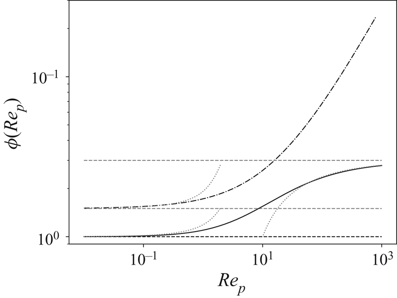
In figure 1, the above-listed functions $\phi (Re_p)$ are reported against the particle Reynolds number. As shown, the $Re_p$-correction increases faster for the solid sphere case (relation (2.4)) than for the spherical bubble case (relation (2.3)).

Figure 1.

Some correction functions $\phi (Re_p)$ as a function of $Re_p$. For the spherical bubble case: relation (2.3) (continuous black line); the Stokes flow regime $\phi=1$, defined in this paper as the case of reference (relation (2.2)) (black dashed line); the Taylor & Acrivos solution $\phi =1 + Re/8$ (lower left dotted grey line); the Moore relation $\phi (Re_p) = 3 [ 1 - 2.211 Re_p^{-1/2} ]$ (right dotted grey line); and the Levich relation $\phi (Re_p) = 3$ (upper grey dashed line). For the solid sphere case: the Stokes solution $\phi =3/2$ (lower grey dashed line); the Oseen solution $\phi =3/2 (1+ 3 Re/8)$ (upper left dotted grey line); and the Schiller and Naumann solution (2.4) (dash-dotted line).

Rearranging (2.1), one obtains the momentum budget per unit of displaced/accelerated mass (i.e. accounting for the added mass effect) as

(2.5)\begin{equation} d_t \boldsymbol{u}_p = \frac{12 \nu }{d_p^{2} ( \rho_p / \rho_f + C_M)} \phi(Re) (\boldsymbol{u}_f-\boldsymbol{u}_p) + \beta D_t \boldsymbol{u}_f , \end{equation}

with $\beta = (1+C_M)/(\rho _p / \rho _f + C_M)$ that compares the mass subject to the total fluid acceleration to the accelerated mass (Calzavarini et al. Reference Calzavarini, Kerscher, Lohse and Toschi2008; Toschi & Bodenschatz Reference Toschi and Bodenschatz2009; Mathai, Lohse & Sun Reference Mathai, Lohse and Sun2020). In the following, the first and second terms on the left-hand side representing the drag and fluid inertia forces per unit of accelerated mass will be denoted by $\boldsymbol {F}_D$ ($\boldsymbol {F}_D=\boldsymbol {f}_D/(m_p + C_M m_f$)) and $\boldsymbol {F}_I$, respectively.

Based on (2.5), the characteristic particle relaxation time is defined as

(2.6)\begin{equation} \tau_p = \dfrac{1}{12} \left(\frac{\rho_p }{ \rho_f} +C_M\right)\dfrac{d_p^{2}}{\nu}. \end{equation}

The Stokes number is then defined as the ratio between $\tau _p$ and the dissipative time scale of the flow $\tau _\eta$

(2.7)\begin{equation} St = \frac{\tau_p}{ \tau_\eta} = \dfrac{ 1}{12 } \left( \frac{\rho_p }{ \rho_f} +C_M\right) \left( \frac{d_p}{\eta}\right)^{2}, \end{equation}

with $\eta$ the dissipative length scale of the turbulence. Note that the factor $1/12$ in (2.6) and (2.7) is common for clean spherical bubbles in the limit $Re_p \rightarrow 0$, whereas, for solid particles, one usually has $1/18$. Indeed, the change of stress condition at the interface is trivially accounted for by rescaling the Stokes number $St$ as $St \rightarrow 2/3 St$ when changing from a free-slip to a no-slip condition keeping the same flow conditions unchanged.

Accordingly, the non-dimensionalizing of the particle equation of motion by a reference velocity and the time scale $\tau _\eta$ reads

(2.8)\begin{equation} d_t\boldsymbol{u}_p = \phi(Re_p) \frac{\boldsymbol{u}_{f}-\boldsymbol{u}_p}{St} + \beta D_t\boldsymbol{u}_f . \end{equation}

As indicated by this equation, as $\phi (Re_p) \geqslant 1$, we expect to observe a faster response of the particles when considering finite Reynolds number effects.

In order for the above equation of motion to be valid, it is essential to consider that the flow around the particle is uniform at the particle scale. Therefore, in the context of homogeneous turbulence as considered in this study, we assume that the diameter of the particle remains sufficiently small compared with the scale of the smallest eddies. In practice, according to Calzavarini et al. (Reference Calzavarini, Volk, Bourgoin, Lévêque, Pinton and Toschi2009), it is sufficient to have $d_p/\eta <10$.

The details of the numerical methods have been presented in Zhang et al. (Reference Zhang, Legendre and Zamansky2019). For the carrier phase, the homogeneous and isotropic turbulence is solved using a pseudo-spectral method with the large-scale forcing proposed by Kumar, Schumacher & Shaw (Reference Kumar, Schumacher and Shaw2014) given a Taylor scale Reynolds number of $Re_\lambda = 100$. A Lagrangian one-way coupling point-particle approach is considered for the particles with a Hermite interpolation scheme of the Eulerian field at the particle position. The flow conditions reported in table 1 are identical for the simulations of each type of particle considered. In the following, we analyse the effect of the finite Reynolds number for light spherical particles (bubble or solid particle) imposing $\rho _p / \rho _f = 0$ and $C_M = 0.5$, giving $\beta = 3$. For each set of simulations, we consider seven classes of particles with Stokes number ranging from 0.02 to 2, as listed in table 2.

Table 1.

The simulation parameters for the turbulent flow field. The number of grid points in each direction is $N$, $H = 2{\rm \pi}$ the size of numerical domain, $T_L = (2/3\mathcal {K})/\varepsilon$ the eddy turnover time, $L = (2/3 \mathcal {K})^{3/2} /\varepsilon$ the scale of the large eddies, $\mathcal {K}$ the average turbulent kinetic energy and $\varepsilon$ the average dissipation rate; $Re_H=H \sqrt (2/3\mathcal {K})/\nu$ is the Reynolds number based on the size of the computational domain, $Re_\lambda$ is the Reynolds number based on the Taylor length scale, $\eta$ and $\tau _\eta$ are the Kolmogorov length and time scales; $Re_0 = (\tau _L/\tau _\eta )^{2}$ is the square of the ratio of the Lagrangian integral time scale to the Kolmogorov time scale; $\varDelta$ and $\Delta t$ are the grid size and the time step of the simulation.

Table 2.

The non-dimensional diameter of the particles $d_p/\eta$ and their Stokes number $St$.

In § 3, we investigate the finite Reynolds number effects on the dynamics of particles. For this, we consider for $\phi (Re_p)$ the expressions (2.2) (the case of reference with $\phi (Re_p)=1$), (2.3) (the spherical bubble case) and (2.4) (the solid sphere case).

3. Finite Reynolds number effects and effective Stokes number

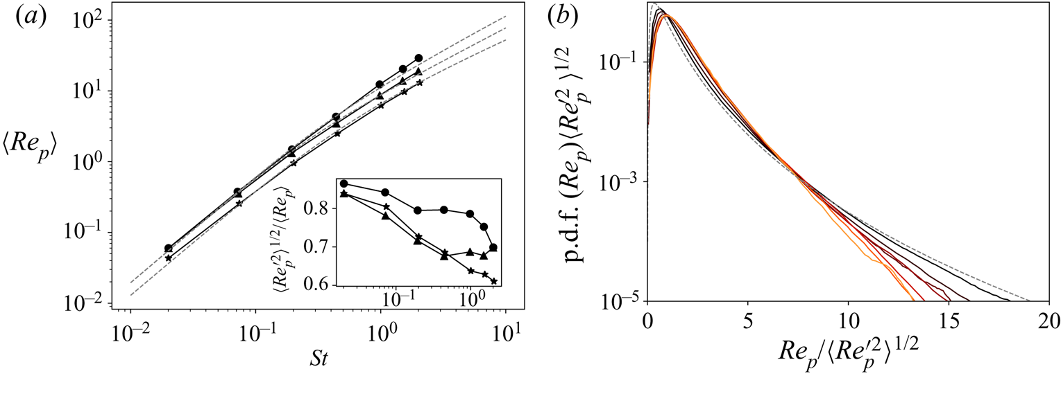
For the set of numerical simulations described in tables 1 and 2, we first report the statistics of the particle Reynolds number. Figure 2 shows the evolution of the mean and root-mean-square of the particle Reynolds number $Re_p$ with $St$. As expected, for the three $\phi (Re_p)$ relations considered, the average value of the Reynolds number $\langle Re_p \rangle$ increases with the Stokes number. For $St>1$, it appears that the average Reynolds number can be significantly larger than 1, which indicates that finite Reynolds number effects have a significant impact and should be accounted for. Indeed, we remark that the differences between the use of relation (2.2) or (2.3) are sizable at sufficiently large Stokes numbers, with a reduction of the relative velocity due to the Reynolds number effect. For the maximum Stokes number considered here, $\langle Re_p \rangle \approx 30$, when considering no $Re_p$-correction while $\langle Re_p \rangle \approx 20$ and $\langle Re_p \rangle \approx 10$ for spherical bubble ($Re_p$-correction (2.3)) and solid sphere ($Re_p$-correction (2.4)) cases, respectively. As well, the relative velocity of a solid sphere is significantly reduced compared with a spherical bubble under the same flow conditions. We also remark in the inset of figure 2(a) that the standard deviation of the Reynolds number is of the order of its average value.

Figure 2.

(a) Evolution of the mean particle Reynolds number with the Stokes number, for the three drag law considered here. Symbols represent the DNS, ($\circ$) the reference case $\phi (Re_p)=1$, ($\triangle$) spherical bubble case $\phi (Re_p)$ given by relation (2.3), ($*$) solid sphere case $\phi (Re_p)$ given by relation (2.4). The grey dashed line corresponds to the prediction of the Reynolds number proposed in (4.9). Inset: ratio of the standard deviation of the particle Reynolds number to its average. (b) The p.d.f. of $Re_p$ for different $St$ normalized by its standard deviation. For the case of the drag from Mei (2.3). Curves from black to orange correspond to an increase of the Stokes number. The dashed line is the log-normal distribution with parameters $\sigma ^{2}=\ln 2, \mu =-\sigma ^{2}/2$, such that the mean and root-mean-square values are both unity.

In figure 2(b), we report the probability distribution function (p.d.f.) of the Reynolds number when considering the $Re_p$-correction for the spherical bubble case (relation (2.3)). It is observed that the normalized p.d.f. is quite close to a log-normal distribution, and that the instantaneous Reynolds number can present deviations significantly larger than its root-mean-square. For $St\rightarrow 0$, the drag force and fluid inertia force are proportional (Zhang et al. Reference Zhang, Legendre and Zamansky2019), leading the particle Reynolds number to be proportional to the norm of the fluid acceleration at the particle position: $Re_p = ({d}/{\nu })\tau _p |1-\beta | |D_t\boldsymbol {u}_f|$. Therefore, the log-normal distribution of $Re_p$ is expected since the fluid acceleration norm is well described by this distribution (Yeung et al. Reference Yeung, Pope, Lamorgese and Donzis2006; Toschi & Bodenschatz Reference Toschi and Bodenschatz2009). It is further observed that the normalized p.d.f. of $Re_p$ depends slightly on the Stokes number, with a reduced probability of observing large $Re_p$ fluctuations with increasing $St$. Note also that, for the two other considered cases, the behaviour (not presented in figure 2 for clarity) is very similar.

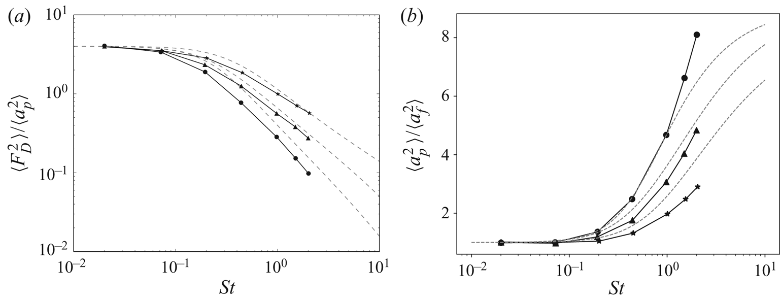
We present in figure 3 the variance of the drag forces per unit of accelerated mass $\boldsymbol{F}_D$ for the three different drag laws considered. Despite the increase of the relative velocity reported above, we observe that $\boldsymbol{F}_D$ is reduced when the Stokes number increases. We notice further that considering the $Re_p$-correction (2.3) gives a slower reduction compared with the case of reference $\phi (Re_p)=1$. From the definition of the Reynolds number and of the Stokes number, $\boldsymbol{F}_D^{2}$ normalized by the square of the Kolmogorov acceleration $a_\eta ^{2}$ can be expressed as

(3.1)\begin{equation} \dfrac{ \boldsymbol{F}_D^{2}}{ a_\eta^{2}} = \phi^{2}(Re_p)Re_p^{2} \dfrac{\rho_p / \rho_f +C_M}{12} St^{{-}3}. \end{equation}

As indicated by this expression, if the quantity $\langle \phi ^{2}(Re_p)Re_p^{2} \rangle$ grows with $St$ less rapidly than $St^{3}$, then the variance of ${\boldsymbol{F}_D^{2}}/{ a_\eta ^{2}}$ decreases as the Stokes number increases, as observed in figure 3. When considering the solid sphere case, which presents the strongest increase of the correction function $\phi$ with $Re_p$, this imposes that $\langle Re_p \rangle$ grows approximately slower than linearly, as already observed in figure 2.

Figure 3.

Variance of the drag force normalized by the variance of the particle acceleration (a) and variance of the acceleration normalized by the acceleration variance of fluid particles (b) as a function of the Stokes number $St$; ($\circ$) obtained for a clean bubble in the Stokes flow regime (2.2), ($\Delta$) for clean bubbles (2.3) and ($*$) for solid particles (2.4). The dashed lines correspond to expressions (4.5) and (4.7).

In figure 3 we also report the particle acceleration variance $\langle \boldsymbol{a}_p^{2} \rangle$. It is observed that, for the three drag laws considered, the acceleration variance normalized by the fluid acceleration variance $\langle \boldsymbol{a}_f^{2} \rangle$ increases with the Stokes number, essentially due to the progressive fading of the drag force as well as its decorrelation with the fluid inertia force, as explained by Zhang et al. (Reference Zhang, Legendre and Zamansky2019). Note that further increase of the Stokes number would lead to a saturation of the normalized acceleration variance to $\beta ^{2}$, as shown by Calzavarini et al. (Reference Calzavarini, Volk, Bourgoin, Lévêque, Pinton and Toschi2009) and Zhang et al. (Reference Zhang, Legendre and Zamansky2019), but in this case the particle diameter would be too large for the pointwise particle approach to remain valid. The case of reference $\phi (Re_p)=1$ gives to a faster increase of the acceleration variance and for the case of spherical bubbles it increases faster than for the solid sphere case.

To characterize the inertia effects on the particle response time through the drag force correction $\phi (Re_p)$, we decompose the particle Reynolds number into its mean and fluctuating parts, $Re_p = \langle Re_p \rangle + Re_p'$ and approximate the drag force per unit of accelerated mass using a Taylor expansion of the function $\phi$ around $\phi (\langle Re_p \rangle )$

(3.2)\begin{equation} \boldsymbol{F}_D = \phi(\langle Re_p \rangle) \dfrac{\boldsymbol{u}_f-\boldsymbol{u}_p}{\tau_p} + Re_p' \phi'(\langle Re_p \rangle) \dfrac{\boldsymbol{u}_f-\boldsymbol{u}_p}{\tau_p} + \ldots ,\end{equation}

with $\phi '$ the derivative of $\phi$ with respect to $Re_p$. This relation leads to the introduction of an effective relaxation time $\tau _p^{*}$, as already proposed by Février, Simonin & Squires (Reference Février, Simonin and Squires2005) and Bergougnoux, Bouchet & Lopez (Reference Bergougnoux, Bouchet, Lopez and Guazzelli2014), that accounts for the Reynolds number effects

(3.3)\begin{equation} \tau_p^{*} = \tau_p / \phi(\langle Re_p \rangle). \end{equation}

We further introduce the effective Stokes number as

(3.4)\begin{equation} St_* = St / \phi(\langle Re_p \rangle). \end{equation}

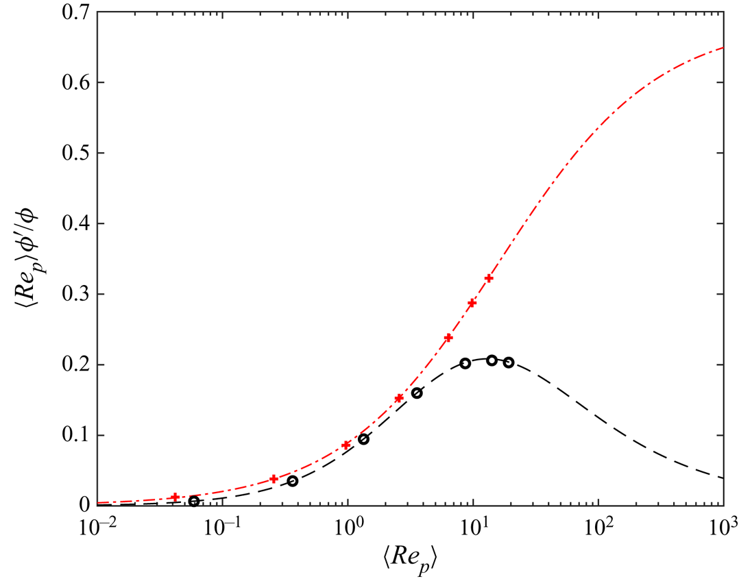
Despite the particle Reynolds number presenting large fluctuations, the Taylor expansion can be truncated at first order as far as one is concerned with low-order statistics. To justify this assertion, we compare the magnitude of the second-order and the first-order terms in (3.2). We plot in figure 4 the ratio $\langle Re_p \rangle \phi '(\langle Re_p \rangle ) / \phi (\langle Re_p\rangle )$ against $\langle Re_p \rangle$ for the two $Re_p$-corrections considered here (2.3)–(2.4). Note that this amounts to considering that the order of magnitude of the fluctuations of $Re_p$ as $O(Re'_p) = \langle Re_p \rangle$, consistently with the observation of figure 2. We remark that for the case of reference $\phi '(\langle Re_p \rangle )=0$. We found that, in the simulation for spherical bubbles, the largest value of this ratio is approximately $0.2$ for $St \approx 1.55$ and in the simulation for a solid sphere, the ratio increases monotonically up to its asymptotic value of 0.687 at large $St$. For moderate values of Reynolds number, the second term on the right-hand side of (3.2) remains smaller than the first term.

Figure 4.

Evolution of $({\langle Re_p \rangle }/{\phi (\langle Re_p \rangle )}) \phi '(\langle Re_p \rangle )$ as a function of $\langle Re_p \rangle$. Symbols correspond to the results of the DNS: ($\circ$) for the bubble case with the Mei et al. (Reference Mei, Klausner and Lawrence1994) correction (2.3); ($\times$) for the solid sphere case with the Schiller & Naumann (Reference Schiller and Naumann1933) correction (2.4). The lines are the analytical results corresponding to (2.3) (in red) and (2.4) (in black).

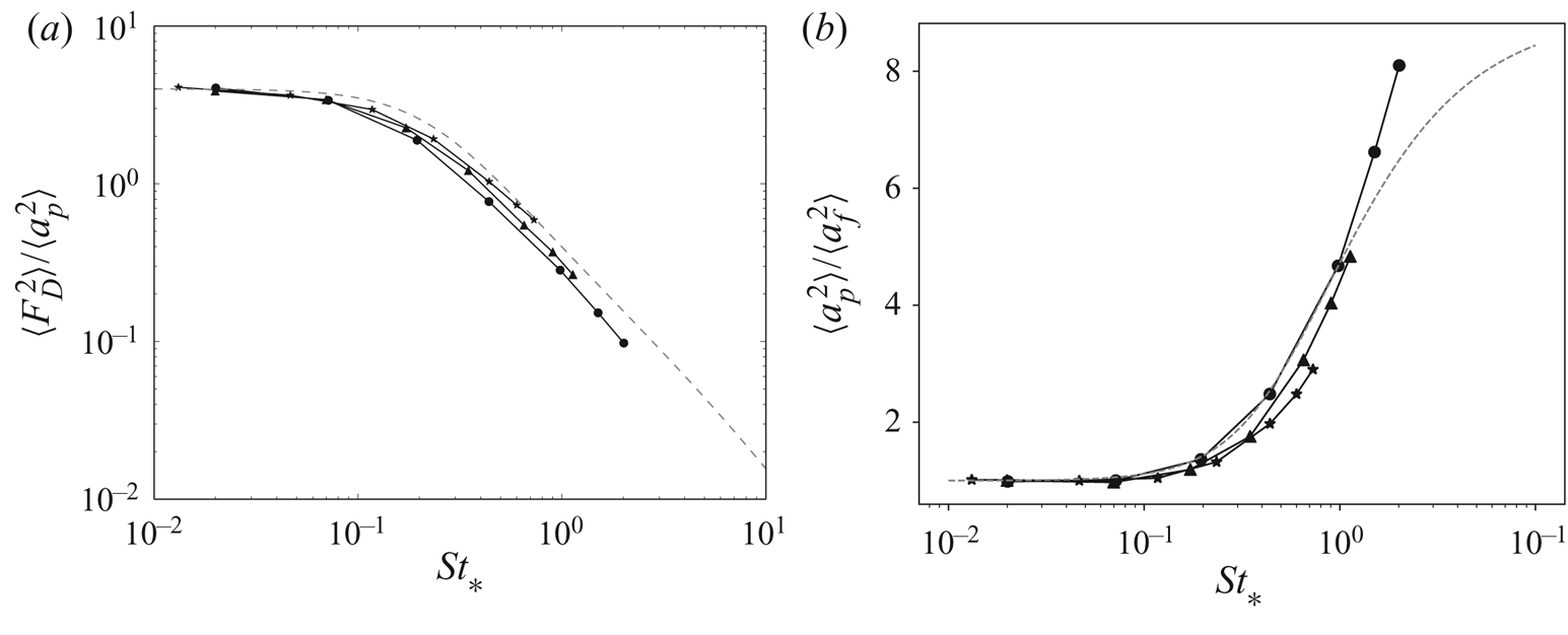
In order to discuss the relevance of $St_*$, we show in figure 5 the evolution of the variance of the drag force and of the particle acceleration for the various simulations as a function of $St_*$. When plotted against $St_*$, these quantities now collapse onto a single curve, compared with what is reported in figure 3 where the evolution is reported against $St$. We recover here the expected effect of the $Re_p$-correction on the drag force: the particle response time to the flow is decreased, thus decreasing the effective Stokes number. We show that the effective Stokes number given by (3.4) is the relevant parameter to describe the inertial flow effect on the particle response to the turbulent flow.

Figure 5.

Variance of the drag force normalized by the variance of the particle acceleration (a) and variance of the acceleration normalized by the acceleration variance of fluid particles (b) as a function of the modified Stokes number $St_*$; ($\circ$) obtained with no $Re_p$-corrections, ($\Delta$) for clean bubbles (2.3) and ($*$) for solid particles (2.4). The dashed lines correspond to the estimation from (4.5) and (4.7).

4. Prediction for the forces applied to the particle and the Reynolds number

Following the approach of Tchen (Reference Tchen1947) (see also Hinze Reference Hinze1975; Mei Reference Mei1996; Alipchenkov & Zaichik Reference Alipchenkov and Zaichik2010), Zhang et al. (Reference Zhang, Legendre and Zamansky2019) estimate the variance of the drag forces, the fluid inertia force and the particle acceleration variance as functions of $St$, $\beta$ and a Reynolds number $Re_0=(\tau _L/\tau _\eta )^{2}$ defined as the square of the ratio of the Lagrangian integral time scale $\tau _L$ to the Kolmogorov time scale, as

(4.1)$$\begin{gather} \dfrac{\langle \boldsymbol{F}_D^{2} \rangle}{a_\eta^{2}} \approx c_0 \frac{(1-\beta)^{2}}{1-St^{2} / Re_0}\left[\frac{\tan^{{-}1}(c_1St)}{c_1St} -\frac{\tan^{{-}1}(c_1Re_0^{1/2})}{c_1Re_0^{1/2}}\right] = \varGamma_D(St,\beta,Re_0), \end{gather}$$

(4.2)$$\begin{gather}\dfrac{\langle \boldsymbol{F}_I^{2} \rangle }{a_\eta^{2}} \approx c_0 \beta^{2}\left[1 -\frac{\tan^{{-}1}(c_1Re_0^{1/2})}{c_1Re_0^{1/2}}\right] = \varGamma_I(St,\beta,Re_0), \end{gather}$$

(4.3)\begin{gather} \dfrac{\langle \boldsymbol{a}_p^{2}\rangle }{a_\eta^{2}} \approx c_0 \left[ \beta^{2} + \dfrac{1-\beta^{2}}{1-St^{2} / Re_0} \dfrac{\tan^{{-}1}( c_1 St)}{ c_1 St} - \dfrac{1-\beta^{2} St^{2} / Re_0}{1-St^{2} / Re_0} \dfrac{\tan^{{-}1}( c_1 Re_0^{1/2})}{ c_1 Re_0^{1/2}} \right] \nonumber\\ \hspace{-18pc}= \varGamma_a(St,\beta,Re_0), \end{gather}

with the parameter $c_1$ found to be $c_1=2.1$; $c_0$ can be interpreted as the ratio of the fluid particle acceleration variance to the square of the Kolmogorov acceleration, and is therefore dependent on the flow Reynolds number, as reported for example by La Porta et al. (Reference La Porta, Voth, Crawford, Alexander and Bodenschatz2001) and Sawford et al. (Reference Sawford, Yeung, Borgas, Vedula, La Porta, Crawford and Bodenschatz2003). Note that $Re_0$ can be approximated as $Re_0 \approx (0.08 Re_{\lambda })^{2}$ (Sawford & Yeung Reference Sawford and Yeung2011; Zhang et al. Reference Zhang, Legendre and Zamansky2019). In (4.1), (4.2) and (4.3) we introduce $\varGamma _D$, $\varGamma _I$ and $\varGamma _a$ as the estimations for $\langle \boldsymbol{F}^{2}_D\rangle / a^{2}_\eta$, $\langle \boldsymbol{F}^{2}_I\rangle / a^{2}_\eta$ and $\langle \boldsymbol{a}^{2}_p\rangle / a^{2}_\eta$, respectively. These expressions are valid for $Re_p \ll 1$ as they are based on a linear response of the particle velocity to the fluid velocity. Further, in the derivation of these expressions, two main assumptions are considered. Firstly, we assume that the Lagrangian fluid velocity spectra along the trajectory can be modelled as (Hinze Reference Hinze1975; Mordant, Metz & Michel Reference Mordant, Metz and Michel2001)

(4.4) \begin{equation} E_f(\omega) = \left\{ \begin{array}{@{}ll} \dfrac{k_0 \tau_L ^{2} \langle \varepsilon \rangle }{( \tau_L \omega) ^{2} + 1} & \mbox{for} \ \omega < k_1 \dfrac{2{\rm \pi}}{\tau_\eta}, \\ 0 & \mbox{for} \ \omega \geqslant k_1 \dfrac{2{\rm \pi}}{\tau_\eta}, \end{array}\right. \end{equation}

which presents saturation for $\omega \ll \tau _L^{-1}$. The coefficients $k_1$ and $k_0$ are such that $c_0= 2 {\rm \pi}k_1 k_0$ and $c_1 = 2 {\rm \pi}k_1$. The second assumption amounts to substituting the material derivative of the fluid velocity at the particle position by the Lagrangian time derivative along the particle trajectory, in order to obtain a close expression depending only on the value of the fluid velocity at the particle position. Zhang et al. (Reference Zhang, Legendre and Zamansky2019) checked that these assumptions are valid in the case of bubbles with a sufficiently small Reynolds number. In particular, it was shown that the first assumption gives a quite accurate acceleration variance although it misses any effect of preferential concentration while the second one requires the Stokes number to be sufficiently small to be valid.

We propose to generalize the relations (4.1)–(4.3) to the cases of particles with a finite Reynolds number. For this, we take into account their nonlinear drag law ($Re_p$-correction) by relying on the effective particle response time introduced in the previous section. Indeed, in view of the similarity of the evolution of the variance of the force and the acceleration as a function of $St_*$, presented in figure 5, we simply propose to replace $St$ by $St_* = St / \phi (\langle Re \rangle )$ in (4.1)–(4.3)

(4.5)$$\begin{align} \dfrac{\langle \boldsymbol{F}_D^{2} \rangle}{a^{2}_\eta} &\approx \varGamma_D(St_*,\beta,Re_0) , \end{align}$$

(4.6)$$\begin{align}\dfrac{\langle \boldsymbol{F}_I^{2} \rangle}{a^{2}_\eta} &\approx \varGamma_I(St_*,\beta,Re_0) , \end{align}$$

(4.7)$$\begin{align}\dfrac{\langle \boldsymbol{a}_p^{2}\rangle}{a^{2}_\eta} &\approx \varGamma_a(St_*,\beta,Re_0) . \end{align}$$

Note that (4.6) is left unchanged, since in our basic approximation the fluid particle acceleration at the particle position does not depend on the Stokes number as preferential concentration effects are discarded, $\varGamma _I(St_*,\beta ,Re_0) = \varGamma _I(\beta ,Re_0)$.

The issue, for the use of these relations, is now to have a prediction for $St_*$, as it requires us to know the average particle Reynolds number $\langle Re_p \rangle$. First of all, we observe in figure 2 that the standard deviation of the Reynolds number is nearly equal to its average, and as a consequence one can write $\langle Re_p \rangle \approx \sqrt {{\langle Re_p^{2} \rangle }/{2}}$. On the other hand, it follows from the previous section that the variance of the drag force can be estimated, at first order, as $\langle \boldsymbol{F}_D^{2} \rangle \approx {\langle (\boldsymbol {u}_p-\boldsymbol {u}_f)^{2} \rangle }/{\tau _p^{*\,2}}$. Substituting in the estimation of the average Reynolds number, we obtain

(4.8)\begin{equation} \langle Re_p \rangle \approx St_* \frac{d_p}{\eta} \sqrt{\frac{1}{2}\frac{\langle \boldsymbol{F}_D^{2} \rangle}{a_\eta^{2}}}. \end{equation}

Further, using the estimate of the drag force variance (4.5) and substituting with the definition of $St_*$ from relation (3.4), we obtain an implicit relation that makes possible the calculation of $\langle Re_p \rangle$

(4.9)\begin{equation} \langle Re_p \rangle \approx \dfrac{St}{\phi(\langle Re_p \rangle)} \dfrac{d_p}{\eta} \left[\dfrac{1}{2} \varGamma_D\left(St/ \phi(\langle Re_p \rangle),\beta,Re_0\right) \right]^{1/2} . \end{equation}

This expression can easily be solved iteratively by taking for example as initial guess $\langle Re_p \rangle = 0$. We present in figure 2 the comparison between the calculation of $\langle Re_p \rangle$ from (4.9) and the values obtained by DNS. It is observed that, for the three drag laws considered here, the estimation of the average particle Reynolds number is close to the DNS value. We also show in figures 3 and 5 the comparison to the DNS for the variances of the drag force and of the particle acceleration for the three drag laws. We can conclude that the relations (4.5)–(4.9) provide overall a good prediction of the variance of the considered quantities. Note that, for $St_* \approx 1$, (4.7) underestimates the acceleration variance but if $St_*$ is further increased we find the saturation of the acceleration variance as presented in Zhang et al. (Reference Zhang, Legendre and Zamansky2019) and Calzavarini et al. (Reference Calzavarini, Volk, Bourgoin, Lévêque, Pinton and Toschi2009).

5. Relevance of fluid inertia force for small particles in turbulent flows

The fluid inertia force is dominant in the dynamics of light particles ($\rho _p/\rho _f \ll 1$). On the other hand, it is usually accepted that, for very dense particles ($\rho _p/\rho _f \gg 1$), the fluid inertia force is unimportant. This suggests that only the density ratio matters to justify neglecting the role of the inertia force in the momentum balance of a particle. Using estimates (4.5) and (4.6) for the drag force and the inertia force, we show in the following that this condition could be more subtle and also depends on the particle size.

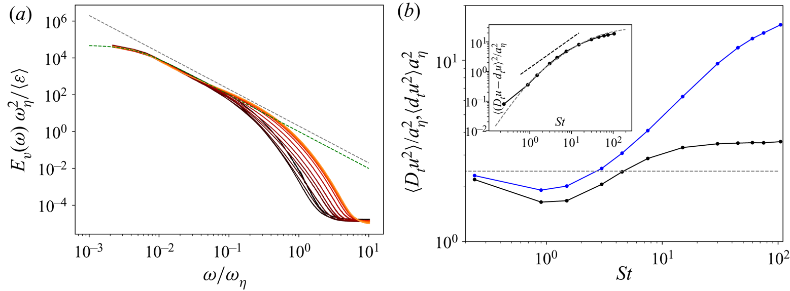
Before using these relations, we first verify that the underlying assumptions, recalled previously and validated for $\rho _p/\rho _f \rightarrow 0$ by Zhang et al. (Reference Zhang, Legendre and Zamansky2019), remain relevant for large density ratios. For this, we show in figure 6 the temporal spectrum of the fluid velocity along the trajectories of solid particles with a high density ratio. To plot this figure we have used data from the DNS of homogeneous isotropic turbulence of Bec et al. (Reference Bec, Biferale, Cencini, Lanotte and Toschi2010) and Lanotte et al. (Reference Lanotte, Calzavarini, Federico, Jeremie, Luca and Massimo2011) obtained for twelve Stokes numbers between $St=0.24$ and $105$ (with $St$ defined as (2.7)) for a homogeneous and isotropic turbulent flow at $Re_\lambda = 400$. For these simulations the solid particles are only subjected to the Stokes drag force (i.e. $\phi (Re_p)=3/2$). We see in this figure that, even for the largest Stokes numbers, the velocity spectrum is well described by relation (4.4). The effect of the Stokes number is only visible at high frequencies.

Figure 6.

(a) Temporal spectra of the fluid velocity along the particle trajectory, for heavy particles only subject to the drag forces with the Stokes drag (i.e. $\phi (Re_p)=3/2$), for $Re_\lambda = 400$ and $St= 0.24$, 0.9, 1.5, 3., 4.5, 7.5, 15, 30, 45, 60, 75, 105, from black to orange respectively from the DNS dataset of Bec et al. (Reference Bec, Biferale, Cencini, Lanotte and Toschi2010) and Lanotte et al. (Reference Lanotte, Calzavarini, Federico, Jeremie, Luca and Massimo2011) in comparison with the power law $\omega ^{-2}$ in grey dashed line and with the model spectra (4.4) in green dashed line. (b) Evolution with $St$ of the variance of the material derivative of the fluid velocity at the particle position $D_t \boldsymbol {u}_f$ (in black) compared to the Lagrangian derivative of the fluid along the particle trajectory $d_t \boldsymbol {u}_f$ (in blue) for heavy particles (same dataset as a). Comparison with the prediction of (4.6) for $\beta ^{2}=1$ in grey dashed line. Inset: variance of $D_t \boldsymbol {u}_f - d_t \boldsymbol {u}_f$ and comparison to $St_*^{2} \langle \boldsymbol{F}_D^{2} \rangle$ computed from relation (4.5).

The second assumption made to derive equations (4.5) and (4.6) neglects the term $(\boldsymbol {u}_p - \boldsymbol {u}_f)\boldsymbol {\cdot } \boldsymbol {\nabla } {\boldsymbol {u}}_f$, in order to identify the material derivative of the fluid velocity $D_t \boldsymbol {u}_f$ with its derivative along particle trajectories $d_t \boldsymbol {u}_f$, $D_t \boldsymbol {u}_f = d_t \boldsymbol {u}_f - (\boldsymbol {u}_p - \boldsymbol {u}_f)\boldsymbol {\cdot } \boldsymbol {\nabla } \boldsymbol {u}_f$. We show in figure 6 that this assumption becomes more and more inaccurate as the Stokes number increases since the particles trajectory diverges from the trajectory of a fluid particle. The difference between $D_t \boldsymbol {u}_f$ and $d_t \boldsymbol {u}_f$ can be estimated by assuming that $(\boldsymbol {u}_p - \boldsymbol {u}_f)$ and $\boldsymbol {\nabla } \boldsymbol {u}_f$ are independent, the first being estimated using relations (3.2) and (4.5) and the second being of the order of $1 / \tau _\eta$, which gives $\langle (D_t \boldsymbol {u}_f - d_t \boldsymbol {u}_f)^{2} \rangle \approx St_*^{2} \langle \boldsymbol{F}_D^{2} \rangle$. In the inset of figure 6 we see that this estimate is relatively accurate, except for the smallest Stokes numbers for which $(\boldsymbol {u}_p-\boldsymbol {u}_f)$ and $\boldsymbol {\nabla } \boldsymbol {u}_f$ are not independent. From this estimate, we conclude that the difference between $D_t \boldsymbol {u}_f$ and $d_t \boldsymbol {u}_f$ remains bounded even for very large Stokes numbers, since $\langle \boldsymbol{F}_D^{2} \rangle$ decreases as $St_*^{-2}$ for $St_*\gg Re_0^{1/2}$. Moreover, it worth remarking that the variance of the material derivative of the fluid velocity at the particle position remains roughly constant when $St$ varies (its variations remain in a $\pm 30\,\%$ range). Therefore relation (4.6), which predicts $\boldsymbol{F}_I$ as independent of $St$, appears to be in agreement with the DNS. This indicates that the two approximations discussed previously tend to compensate each other. Finally, let us mention that in Zhang et al. (Reference Zhang, Legendre and Zamansky2019) it can be checked that relation (4.5) makes a good estimate of the variance of the drag forces for heavy particles.

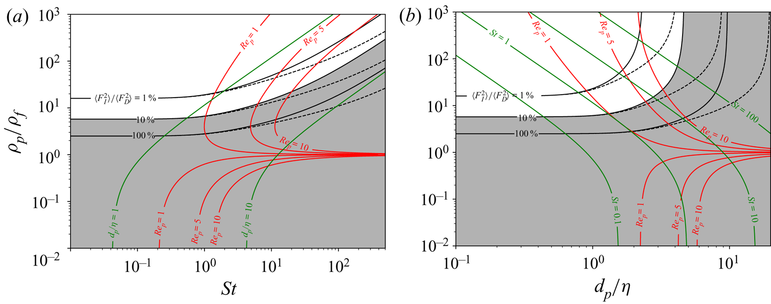
In figure 7, the ratio of $\langle \boldsymbol{F}_I^{2}\rangle /\langle \boldsymbol{F}_D^{2}\rangle$ estimated from (4.5) and (4.6) is plotted for a range of density ratios and particle sizes. For this figure we have selected the $Re_p$-correction (2.4) corresponding to the drag force of a solid sphere given by the relation of Schiller and Neuman. We plot 3 levels of the force ratio $\langle \boldsymbol{F}_I^{2}\rangle /\langle \boldsymbol{F}_D^{2}\rangle = 1\,\%$, 10 % and 100 % vs $\rho _p/\rho _f$ and $St$ in figure 7(a). In this plot, the region of the parameter map for which it is important to account for the fluid inertia forces is shaded in grey. This region is arbitrarily delimited by the curve corresponding to $\langle \boldsymbol{F}_I^{2}\rangle /\langle \boldsymbol{F}_D^{2}\rangle = 10\,\%$. It should be noted that the intermittency is not taken into account, and since the fluid acceleration fluctuations can be much greater than its standard deviation, it tends to further strengthen the effect of the fluid inertia force. Additionally, we plot some levels of the particle Reynolds number as calculated using relation (4.9). As expected, it is observed that, for light particles ($\rho _p/\rho _f<1$), the fluid inertia force is dominant, whereas, for heavy particles, $\rho _p/\rho _f>1$, we observe that the fluid inertia force can be neglected for $\rho _p/\rho _f>10$ and small enough particle diameter, typically $St<1$. However, when the particle Stokes number is increased, the density ratio also needs to be increased in order to neglect the effect of the fluid inertia force. Typically, one needs $\rho _p/\rho _f>100$ for $St=100$. The non-vanishing effect of the fluid inertia force for very heavy but large particles can be simply explained by the observation that, at first order, the fluid inertia force (per unit of displaced mass) is independent of the particles size, as long as the finite size effects can be ignored, while the magnitude of the drag force (per unit of displaced mass) decreases with the particle size, as shown in figure 3.

Figure 7.

Diagram reporting the evolution of $\langle \boldsymbol{F}_I^{2}\rangle / \langle \boldsymbol{F}_D^{2}\rangle$. Iso-values 0.01, 0.1 and 1. of the ratio estimated by (4.5) and (4.6) for $Re_\lambda = 100$ (continuous black lines) and $Re_\lambda =400$ (dashed lines) as a function of $\rho _p/\rho _f$ and $St$ (a) and as a function of $\rho _p/\rho _f$ and $d_p/\eta$ (b). The red lines indicate iso-values of the particles Reynolds number from (4.9) for $Re_\lambda =100$. Green lines give iso-values of $d_p/\eta$ (a) and of $St$ (b). The region of the map where $\langle \boldsymbol{F}_I^{2}\rangle / \langle \boldsymbol{F}_D^{2}\rangle >0.1$ is shaded.

Furthermore, considering the plot against $\rho _p/\rho _f$ and $d_p/\eta$ given in figure 7(b), we can remark that, at $Re_\lambda =100$ for particles of size $d_p/\eta \approx 3$, the inertia force remains important even for very large density ratios. This observation depends on the Reynolds number of the flow. Indeed, for $Re_\lambda =400$, the fluid inertia force should not be neglected for a particle larger than $d_p/\eta \approx 7$. Since it was proposed by Calzavarini et al. (Reference Calzavarini, Volk, Bourgoin, Lévêque, Pinton and Toschi2009) that the finite size effect can be disregarded for particles smaller than $d_p/\eta \approx 10$, the results presented in this section points out that the added mass force can turn out to be of the order of magnitude of the drag force, when the particle inertia becomes important, even for high density ratios. It is interesting to note that the occurrence of this range of size for which the fluid inertia force might be important is also the limit of the validity of the pointwise particle approach. Indeed, for larger particles ($d_p/\eta > 10$) one should account for the finite size effect, probably by considering the filtering at the scale of the particles of the fluid inertia force as proposed by Calzavarini et al. (Reference Calzavarini, Volk, Bourgoin, Lévêque, Pinton and Toschi2009), as well as the additional agitation caused by the turbulent structure of the flow around the particles by introducing a random drag coefficient (Gorokhovski & Zamansky Reference Gorokhovski and Zamansky2018), which leads both variances of the drag force and of the inertia force to scale as $a_\eta ^{2} (d/\eta )^{-2/3}$ (without accounting for the intermittency correction) as shown from the experimental results presented by Voth et al. (Reference Voth, La Porta, Grawford, Alexander and Bodenschatz2002), Qureshi et al. (Reference Qureshi, Arrieta, Baudet, Cartellier, Gagne and Bourgoin2008) and Volk et al. (Reference Volk, Calzavarini, Lévêque and Pinton2011).