1. Introduction

Cox (Reference Cox1958) and Lindley (Reference Lindley1972) have shown that the practice of testing all hypotheses at the same level, regardless of the distribution of the data, can lead to inadmissibility and incompatibility with Bayesian decision theory. One of the most compelling arguments for Bayesian decision theory and the use of probability to model uncertainty is the “Dutch Book” argument, which says that if you are willing to accept either side of each bet implied by your statements and finite combinations of these together, either

1. (a) those statements are “coherent,” that is they comport with the axioms of probability, or

2. (b) a gambler betting against you can choose bets so that you are a sure loser.

Excellent introductions to the concepts of coherence and Dutch Book can be found in Shimony (Reference Shimony1955), Freedman and Purves (Reference Freedman and Purves1969), and de Finetti (Reference de Finetti1974, Section 3.3).

As a practical matter, it is very difficult to structure one's statements of probabilities (i.e. previsions) in such a way that they both reflect one's beliefs and are coherent (see Kadane and Wolfson Reference Kadane and Wolfson1998). Yet the dichotomy above does not allow for discussion of what sets of previsions may be “very” incoherent or just “slightly” incoherent. This paper explores a remedy for this by studying how quickly an incoherent bookie can be forced to lose money. A faster rate of sure financial decline to the bookie, or a faster rate of guaranteed profit to the gambler, is associated with a greater degree of incoherence.

The problem as stated so far requires some normalization. Suppose that a particular combination of gambles yields a sure loss y for the bookie. Then multiplying each gamble by the same constant k > 0 will create a combination of gambles that yields sure loss ky. In this paper we explore how to perform the normalization from the bookie's perspective. We introduce normalizations in Section 3. To fix ideas, however, consider that the bookie cannot be assumed to have infinite resources. A wise gambler would want to be sure that the bookie could cover all the bets. One way to do this would be to require the bookie to escrow the maximum amount that the bookie could lose on each gamble separately. Thus we can ask how much the bookie can be forced to lose for sure, given a specified level of escrow that the bookie can offer. In Section 4, we apply these ideas to assess the incoherence of the practice of fixed level hypothesis testing.

2. Gambles and Incoherence

Think of a random variable X as a function from some space T of possibilities to the real numbers. We assume that, for a bounded random variable X, a bookie might announce some value of x such that he/she finds acceptable all gambles whose net payoff to the bookie is α(X − y) for α > 0 and y < x. Each such x will be called a lower prevision for X. In addition, or alternatively, the bookie may announce some value of x such that the gamble α(X − y) is acceptable when α < 0 and y > x. These x will be called upper previsions for X. We allow that the bookie might announce only upper previsions or only lower previsions or both. For example, if X is the indicator I _A of an event A the bookie might announce that he/she finds acceptable all gambles of the form α(I _A − y) for y < p if α > 0 but no other gambles, in particular, not for y = p. It will turn out not to matter for any of our results whether or not the bookie finds the gamble α(I _A − p) acceptable. In the special case in which x is both an upper prevision and a lower prevision, we call x a prevision of X and denote it P(X). Readers interested in a thorough discussion of upper and lower previsions should refer to Walley (Reference Walley1991).

It will be convenient to assume that, whenever both an upper prevision x ⁺ and a lower prevision x ⁻ have been assessed for the same random variable X, x ⁻ ≤ x ⁺, otherwise the bookie is willing to sell X for a certain price and then buy it right back for a higher price. Although such incoherence could be measured, it requires cumbersome bookkeeping that makes general results difficult to understand. (See Examples 4 and 5 of Schervish et al. Reference Schervish, Seidenfeld and Kadane1999.) In particular, this assumption implies that there can be at most one prevision of X.

A collection x ₁, … , x _n of upper and/or lower previsions for X ₁, … , X _n respectively is incoherent if there exists ∊ > 0 and a collection of acceptable gambles $\{ \alpha _{i}(X_{i}-y_{i}) \} ^{n}_{i=1}$ such that

in which case we say that a Dutch Book has been made against the bookie. Of course, we would need α_i > 0 and y _i < x _i if x _i is a lower prevision for X _i and we would need α_i < 0 and y _i > x _i if x _i is an upper prevision for X _i. When a collection of upper and/or lower previsions is incoherent, we would like to be able to measure how incoherent they are. As we noted earlier, the ∊ in (1) is not a good measure because we could make ∊ twice as big by multiplying all of the α_i in (1) by 2, but the previsions would be the same. Instead, we need to determine some measure of the sizes of the gambles and then consider the left-hand side of (1) relative to the total size of the combination of gambles. This is what we do in Section 3.

3. Normalizations

To begin, consider a single acceptable gamble such as Y = α (X − y). There are a number of possible ways to measure the size of Y. For example sup_t | Y(t)| or sup_t − Y(t) might be suitable measures. This last one has a nice interpretation. It is the most that the bookie can lose on the one particular gamble. It measures a gamble by its extreme value in the same spirit as Dutch Book measures incoherence in terms of an extreme value (the minimum payoff to the gambler) of a combination of gambles. Alternatively, if we think of the gambler and bookie as adversaries with regard to this one gamble Y, the gambler might want to be sure that the bookie will be able to pay up when the bet is settled. We could imagine that the gambler requests that the bookie place funds in escrow to cover the maximum possible loss. So, for the remainder of the paper, we will call e(Y) = sup_t − Y(t) the escrow for gamble Y. Note that e(cY) = ce(Y) for all c > 0. We use the escrow to measure the size of the gamble Y.

When we consider more than one gamble simultaneously, we need to measure the size of the entire collection. We assume that the size of (escrow for) a collection of gambles is some function of the escrows for the individual gambles that make up the collection. That is e(Y ₁, … , Y _n) = f _n(e(Y ₁), … , e(Y _n)). In order for a function to be an appropriate measure of size, we have a few requirements. First,

Equation (2) says that the function f _n must be homogeneous of degree 1 in its arguments so that scaling up all the gambles by the same amount will scale the escrow by that amount as well. Second, since we are not concerned with the order in which gambles are made, we require

Third, in keeping with the use of escrow to cover bets, we will require that, if a gamble is replaced by one with higher escrow, the total escrow should not go down:

If a gamble requires 0 escrow, we will assume that the total escrow is determined by the other gambles:

Since nobody can lose more than the sum of the maximum possible losses from all of the accepted gambles, we require that

Small changes in the component gambles should produce only small changes in the escrow, so we require that

Finally, since we have already decided how to measure the size of a single gamble, we require

So, if Y ₁, … , Y _n is a collection of gambles, we can set e(Y ₁, … , Y _n) = f _n(e(Y ₁), … , e(Y _n)) for some function f _n satisfying (2)–(8) and call e(Y ₁, … , Y _n) an escrow for the collection of gambles. Every sequence of functions $\{ f_{n}\} ^{\infty }_{n=1}$ that satisfy (2)–(8) leads to its own way of defining escrow. Such a sequence is called an escrow sequence. Each function in the sequence is an escrow function.

We can find a fairly simple form for all escrow sequences. Combining (8), (4), and (5), we see that f _n(x ₁, … , x _n) ≥ max{ x ₁, … , x _n}. From (3), we conclude that f _n is a function of the ordered values x ₍₁₎ ≤ x ₍₂₎ ≤ … ≤ x _(n) of x ₁, … , x _n. That is, f _n(x ₁, … , x _n) = f _n(x ₍₁₎, … , x _(n)). Combining these results with (6), we get

Let λ_n(x ₍₁₎, … , x _(n)) = (f _n(x ₍₁₎, … , x _(n)) − x _(n))/ x _(n) so that

In order to satisfy (5), we need λ_n(0, x ₍₂₎, … , x _(n)) = λ_n−1(x ₍₂₎, … , x _(n)). In order to satisfy (2), λ_n must be invariant under common scale changes for all of its arguments. That is

Every such function can be written as

In order to satisfy (4), we must have γ_n nondecreasing in each of its arguments. In order to satisfy (9), we must have

In summary, every escrow sequence satisfies

for some sequence γ₁, γ₂, … of continuous functions where γ₁ ≡ 0 and for n > 1 the functions satisfy the following properties:

(The last condition is equivalent to f _n being nondecreasing in x _(n).) It is straightforward to show that every sequence that meets this description satisfies (2)–(8), hence we have characterized escrow sequences.

One simple collection of escrow sequences consists of all sequences in which γ _n(y ₁, … , y _n−1) = $\gamma \sum_{i=1}^{n-1}y_{i}$ for some common constant γ ∊ [0,1]. In this case, we get a family of escrow functions:

for each 0 ≤ γ ≤ 1. Another example is γ _n(z ₁, … , z _n−1) = z _n−1 for n > 1. This one makes the total escrow equal to the sum of the two largest individual gamble escrows. Other functions are possible, but we will focus on f _γ,n for 0 ≤ γ ≤ 1. It is easy to see that the two extreme escrow functions correspond to γ = 0 and γ = 1:

We now propose to measure the incoherence of a collection of incoherent previsions based on a normalization by an escrow. For a combination of gambles 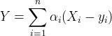$Y=\sum_{i=1}^{n}\alpha _{i}(X_{i}-y_{i}) $ define the guaranteed loss to be G(Y) = −min {0, sup_t∊T Y(t)}. So, Dutch Book can be made if there exists a combination of acceptable gambles whose guaranteed loss is positive. The rate of guaranteed loss relative to a particular escrow function f _n is

where Y _i = α_i(X _i − y _i). Notice that the rate of guaranteed loss is unchanged if all α_i are multiplied by a common positive number. Also, the rate of guaranteed loss is interesting only when Dutch Book is made, otherwise the numerator is 0. The denominator f _n(e(Y ₁), … , e(Y _n)) is 0 if and only if e(Y _i) = 0 for all i. This will occur if and only if the agent who is required to escrow cannot lose any of the individual gambles, in which case the numerator is 0 as well, and we will then define the rate of guaranteed loss to be 0 (since we cannot guarantee loss). The extent of incoherence relative to an escrow and corresponding to a collection of previsions will be the supremum of H(Y) over all combinations Y of acceptable gambles. If the previsions are incoherent then the maximum rate of guaranteed loss is positive, otherwise it is 0.

There is a slightly simpler way to compute the extent of incoherence corresponding to a finite set of previsions than directly from the definition.

Theorem 1. Let x ₁, … , x _n be a collection of incoherent upper and/or lower previsions for X ₁, … , X _n. Define

Then the rate of incoherence is

or equivalently

The supremum and infimum are taken over those α_i that have the appropriate signs.

As with all of the more lengthy proofs in this paper, the proof of Theorem 1 is in Schervish et al. (Reference Schervish, Seidenfeld and Kadane1999). Theorem 1 allows us to ignore the fact that the gamble α(X − x) might not be acceptable when x is a lower or upper prevision for X if we are proving results concerning the rate of incoherence.

Note that if a collection of gambles satisfies the escrow condition h(α₁, … , α _n) ≤ 1, then every subcollection also satisfies the escrow condition because of (5). Also, note that, since every escrow function f _n is between f _0,n and f _1,n, the maximum and minimum possible rates of incoherence correspond to these two escrows.

When we use the bookie's escrow with e(Y) = sup_t − Y(t) for each individual gamble Y, we call the extent of incoherence the maximum rate of guaranteed loss, since the extent of incoherence is the maximum rate at which the bookie can be forced to lose relative to the particular escrow chosen. We focus on the family of escrows f _γ,n defined in (12). The corresponding maximum rates of guaranteed loss will be donoted ρ_γ.

4. Testing Simple Hypotheses At a Fixed Level

Lindley (Reference Lindley1972, 14) argues that it is incoherent to test all hypotheses at the same level, such as .05. (See also Seidenfeld, Schervish, and Kadane Reference Seidenfeld, Schervish and Kadane1990.) Cox (Reference Cox1958) gave an example of how testing all hypotheses at the same level leads to inadmissibility. In this section, we show how this incoherence and inadmissibility can be measured using the measure of incoherence ρ.

Consider the case of testing a simple hypothesis against a simple alternative. Let f ₀ and f ₁ be two possible densities for a random quantity X, and let f be the “true” density of X. Suppose that we wish to test the hypothesis H ₀ : f = f ₀ versus the alternative H ₁ : f = f ₁. To write this as a decision problem, let the parameter space and the action space both be {0, 1} where action a = 0 corresponds to accepting H ₀ and action a = 1 corresponds to rejecting H ₀. Also, parameter i corresponds to f = f _i for i = 0, 1. Let the loss function have the form

with c ₀, c ₁ > 0. The Neyman-Pearson lemma says that the most powerful tests of their sizes and the Bayes rules with respect to all priors have the form: For some constant k, choose a = 1 if f ₁(x) > kf ₀(x), choose a = 0 if f ₁(x) < kf ₀(x), and do whatever you wish (even randomization) if f ₁(x) = kf ₀(x). Now, suppose that someone chooses a value of k and declares that he/she prefers the corresponding test to all other tests. One could infer from this choice an “implied prior” over the two possibilities f ₀ and f ₁. If Pr(f = f ₀) = p and Pr(f = f ₁) = 1 − p, then the Bayes rule is to choose a = 1 if pc ₀f ₀(x) < (1− p)c ₁f ₁(x), which corresponds to k = pc ₀/[(1− p)c ₁]. So p = c ₁k/(c ₀ + c ₁k).

Of course, a classical statistician who refuses to use prior and posterior probabilities will not acknowledge the implied prior. However, incoherence will arise if two tests about the same parameter imply different priors. We illustrate this with a version of the example of Cox (Reference Cox1958). Since the only part of the loss function that matters is c ₀/ c ₁, let c ₁ = 1. As an example, let f ₀ and f ₁ be normal distributions with different means θ but the same variance σ². Suppose that the hypothesis is H ₀ : θ = 0 versus H ₁ : θ = 1 with c ₀ = 1. (The phenomenon we illustrate here applies more generally as shown in Theorem 2). Suppose that either σ = 1 or σ = 0.3 will be true, but we will not know which until we observe the data. That is, the data consist of the pair (X, σ). Let Pr(σ = 1) = 0.5, so that σ is ancillary. A classical statistician who prefers level 0.05 tests whenever available might think that, after observing σ a conditional level 0.05 test should still be preferred to a test whose conditional level given σ is something else. The most powerful conditional level 0.05 test is to reject H ₀ : θ = 0 if X > 1.645σ. The most powerful marginal level 0.05 test rejects H ₀ if X > 0.5 + 0.9438σ² and is the Bayes rule with respect to the prior Pr(θ = 0) = 0.7199. The marginal power of the Bayes rule is 0.6227, while the marginal power of the conditional level 0.05 test is 0.6069. Since both tests have the same level, the conditional test is inadmissible.

To see how this inadmissibility translates into incoherence, we interpret the preference of one test δ₁ to another δ₂ as a preference for suffering a loss equal to the risk function of δ₁ to suffering a loss equal to the risk function of δ₂. The risk function of a test δ is

To say that δ₁ is preferred to δ₂ means that R(θ, δ₂) − R(θ, δ₁) is an acceptable gamble. In our example, let α_δ(σ) and β_δ(σ) denote the size and power of test δ conditional on σ. Also, let β_cl(σ) denote the power of the most powerful level 0.05 test. Then, for each σ, the classical statistician prefers the level 0.05 test to every other test. So, for each σ and all δ that are not the most powerful level 0.05 test, the following gamble is acceptable, even favorable:

where

In other words, b is an upper or lower prevision for A depending on whether a < 0 or a > 0.

We can make use of the construction in (17) to obtain a general result. Theorem 2 has a technical condition (concerning risk sets) that is known to be satisfied for problems of testing simple hypotheses against simple alternatives using fixed sample size and sequential tests. For more detail on risk sets, see Sections 3.2.4 and 4.3.1 of Schervish (Reference Schervish1995).

Theorem 2. Let θ be a parameter and let the parameter space Ω consist of two points {0, 1}. Consider two decision problems D ₀ and D ₁ both with the same parameter space Ω and with nonnegative loss functions L ₀ and L ₁. Let the data in problem D _i be denoted X _i. Suppose that the risk sets for the two decision problems are closed from below. Suppose that an agent prefers the admissible decision rule δ_i to all others in problem D _i for i = 0, 1. For each decision rule ψ in problem D _i, let R _i(θ, ψ) denote the risk function. Let A = {θ = 0} and define

If ψ is admissible in problem D_i and is not equivalent to δ_i, then

If δ₀ and δ₁ are not Bayes rules with respect to a common prior, then there exist real numbers d ₀ and d ₁ and decision rules ψ₀ (in problem D ₀) and ψ₁ (in problem D ₁) such that the two gambles d ₀a ₀(ψ₀) (I _A − b ₀(ψ₀)) and d ₁a ₁(ψ₁) (I _A − b ₁(ψ₁)) are both acceptable, but

Also,

where the supremum is over all p ₀ > p ₁ such that either δ_i is a Bayes rule with respect to prior p _i for i = 0, 1 or δ_i is a Bayes rule with respect to prior p _1−i for i = 0, 1.

As an example of Theorem 2, return to the test of H ₀ : θ = 0 versus H ₁ : θ = 1 where X ∼ N(θ, σ²) with σ being one of two known values. Let σ_i be the value of σ for problem D _i for i = 0, 1. The implied prior probability of {θ = 0} is k/(c ₀ + k) where k comes from the form of the Neyman-Pearson test and c ₀ comes from the loss function (16). If a classical statistician decides to test the hypothesis H ₀ : θ = 0 at level 0.05 regardless of the value of σ, this will often require choosing two different values of k in the Neyman-Pearson lemma. In fact, k = exp(1.645/σ − 0.5/σ²), and the implied prior is

not a one-to-one function of σ, but highly dependent on σ. In this problem, the lower boundary of the risk set is a strictly convex differentiable function so that every point on the lower boundary has a unique support line and hence a unique prior such that the corresponding rule is Bayes with respect to that prior. This means that the sup in (21) is unnecessary and

if p(σ₀) > p(σ₁) with a similar formula if p(σ₀) < p(σ₁). For the case of γ = 1, this simplifies to

In this case, the degree of incoherence is a simple monotone function of how far apart the implied priors are for the two level 0.05 tests. Theorem 2 would also apply if one or both of the two decision problems were a sequential decision problem in which the loss equals the cost of observations plus the cost of terminal decision error.

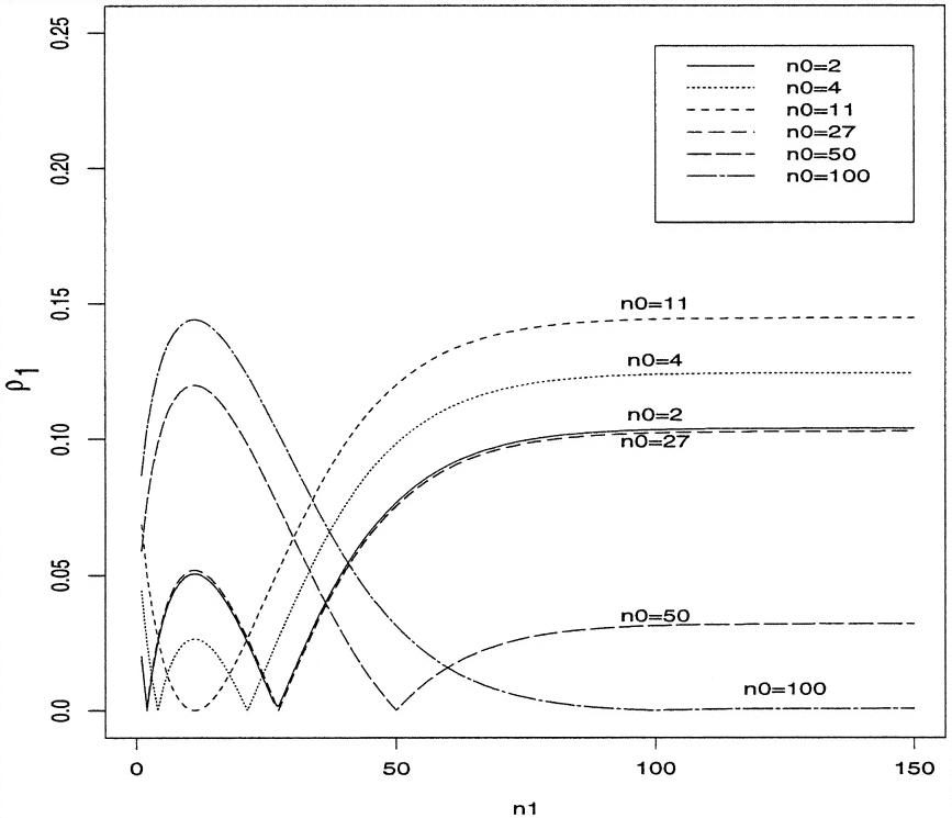
It is interesting to examine the relationship between ρ_γ and the pair (σ₀, σ₁). For example, suppose that σ_i = 2/√ n _i for two different values n ₀ and n ₁. This would correspond to the data consisting of a sample X ₁, … , $X_{n_{i}}$ of independent normal random variables with mean θ and variance 4, where the sample size is n _i in decision problem D _i. Figure 1 is a plot of ρ_γ as a function of (n ₀, n ₁) for the case γ = 1 and c ₀ = 19. Other values of γ produce plots with similar appearances. Of course the values of ρ_γ are higher for γ < 1. We chose c ₀ = 19 to correspond to the classical choice of α = 0.05. Each curve in Figure 1 corresponds to a fixed value of n ₀ and lets n ₁ vary from 1 to 150. Notice that each curve touches 0 where n ₁ = n ₀ since there is no incoherence in that case. Some of the curves come close to 0 in another location as well. For example, the n ₀ = 27 curve comes close to 0 near n ₁ = 2 and the n ₀ = 2 curve comes close to 0 near n ₁ = 27. The reason is that the implied priors corresponding to σ = 2/√2 and σ = 2/√27 are nearly the same (0.7137 and 0.7107 respectively), making these two level 0.05 tests nearly coherent. Indeed, the entire curves corresponding to n ₀ = 2 and n ₀ = 27 are nearly identical for this same reason. Another interesting feature of Figure 1 is that all of the curves are rising as n ₁ → ∞ but not to the same level. As n ₁ → ∞, the implied prior on A = {θ = 0} converges to 0. But if n ₀ is large also, then the implied prior corresponding to σ = 2/√ n ₀ is also close to 0. For example, with n ₀ = 100, the implied prior is 7.3 × 10⁻⁴. There is not much room for incoherence between 0 and 7.3 × 10⁻⁴, so the curve corresponding to n ₀ = 100 will not rise very high. On the other hand, with n ₀ = 11, the implied prior is 0.1691, leaving lots of room for incoherence. In fact, since 0.1691 is the largest possible implied prior in this example, all of the other curves have local maxima near n ₁ = 11, and the n ₀ = 11 curve rises higher than all the others as n ₁ increases. Since the limiting implied prior is 0 as n ₁ → ∞, the height to which the n ₀ curve rises as n ₁ increases is

The curve corresponding to n ₀ = 4 illustrates the original example of Cox (Reference Cox1958), in which the alternative is that θ equals the larger of the two different standard deviations.

Figure 1.

Plot of ρ₁ for level 0.05 testing as a function of n₁ (running from 1 to 150) for various values of n₀ with c₀ = 19.

Lehmann (Reference Lehmann1958) offered a rule of thumb for choosing tests based on both their size and their power. One chooses a postive number λ (such as c ₀ in the loss function (16)) and then chooses the test so that the probability of type II error equals λ times the probability of type I error. In our case of testing one normal distribution against another one with the same variance σ², this procedure will produce the minimax rule with loss (16) if λ = c ₀. When λ = 1, it is easy to check that Lehmann's suggestion is the Bayes rule with respect to the prior with Pr(θ = 0) = 1/(1 + c ₀) for all σ. In this special case ρ_γ = 0 for all γ. However, when λ ≠ 1, each σ leads to a Bayes rule with respect to a different implied prior. Assuming that the test will be to reject H ₀ if X > y, one must solve the equation

The implied prior, assuming, still, that the loss is (16), is then

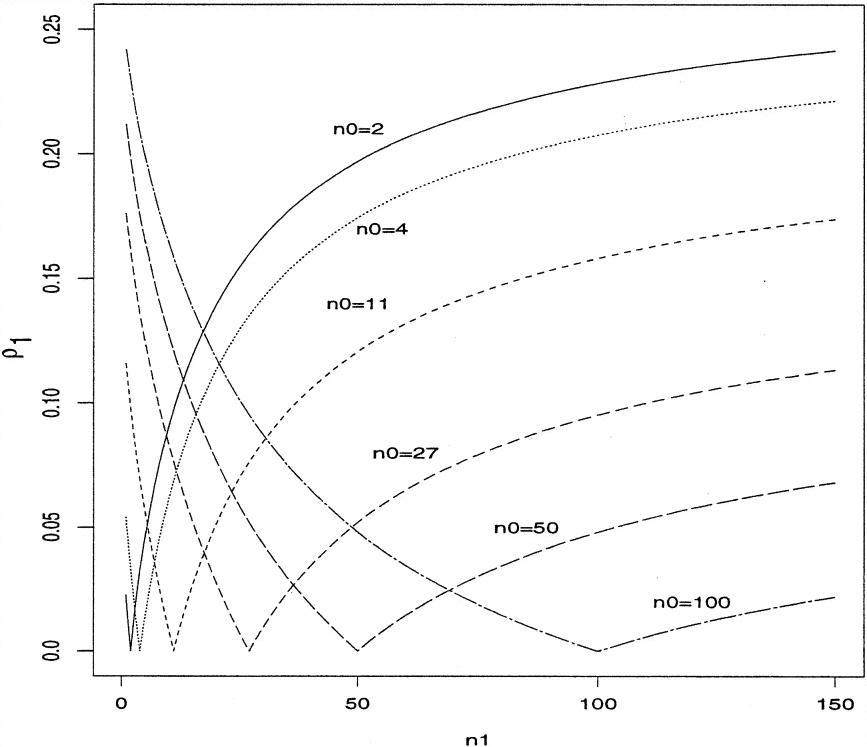
When λ = 1, y = 1/2 solves (23). Plugging this into (24) yields p _L (σ) = 1/(1 + c ₀) for all σ as we noted earlier. Two other limiting cases are of interest. If σ → ∞, then y/σ must converge to Φ⁻¹ (λ/[1 + λ]) in order for (23) to hold. This would make the type I error probability 1/(1 + λ), and the limit of p _L(σ) would be 1/(1 + c ₀). It is not difficult to see that the type I error probability is highest for σ = ∞, so it must be less than 1/(1 + λ) for all finite σ. If σ → 0, then (y − 1/2)/σ² must converge to log(λ) in order for (23) to hold. In this case, p _L (σ) converges to λ/(λ + c ₀). For the case of λ = c ₀ = 19, Figure 2 shows the value of ρ₁ with σ_i = 2/√ n _i for i = 0, 1 for various values of n ₀ and n ₁ in the same spirit (and on the same vertical scale) as Figure 1.

Figure 2.

Plot of ρ₁ for minimax rule with c₀ = 19 as a function of n₁ (running from 1 to 150) for various values of n₀.

The curves in Figure 2 are higher for large n ₁ than the corresponding curves in Figure 1. This means that, when c ₀ = 19, Lehmann's procedure with λ = 19 is more incoherent (as measured by ρ₁) for large values of n ₁ than testing at level 0.05. Lehmann (Reference Lehmann1958) made his suggestion for testing, not to be more coherent than fixed level testing, but rather to avoid a different problem exhibited by fixed level testing. Testing all hypotheses at the same level, regardless of how much data one has, allows the probability of type II error to become much smaller than the probability of type I error as the sample size increases. This amounts to behaving as if the null hypothesis were not very important compared to the alternative. Indeed, the fact that the implied prior goes to zero as the sample size increases reflects this fact. Lehmann's procedure forces the type I and type II errors to decrease together as sample size increases, thereby making sure that both the null and the alternative remain important as the sample size increases. In fact, the implied prior approaches a value strictly between 0 and 1 as sample size increases. What makes Lehmann's procedure less coherent than fixed level testing is the rate at which the implied prior approaches its limit as sample size increases. For Lehmann's procedure, the implied prior differs from its limit by approximately a constant divided by sample size whereas the implied prior for a fixed level test differs from 0 by approximately exp(− cn) for some constant c. In this simple testing problem, Lehmann's procedure with λ = 1 leads to coherent choices of admissible tests for all sample sizes. Lehmann's procedure with λ = 1 here corresponds to an implied prior for the null hypothesis of 1/(1 + c ₀) = 0.05 when c ₀ = 19, and an implied prior of 1/2 when losses are equal (c ₀ = 1). As we noted, Lehmann's rule gives the minimax risk solution for λ = c ₀. However, as Lindley (Reference Lindley1972, 14) points out, it is not guaranteed that minimax risk solutions from different families of admissible tests correspond to the same Bayes model. In our testing problem, this is what happens with Lehmann's rule when λ ≠ 1, which explains how it suffers a positive degree of incoherence. An alternative procedure to Lehmann's which also lets type I and type II error probabilities decrease as sample size increases, but which is coherent, is to minimize a positive linear combination of those error probabilities.

5. Summary

In this article we introduce a familiy of indices of incoherence of previsions, based on the gambling framework of de Finetti (Reference de Finetti1974). When a bookie is incoherent, a gambler can choose a collection of gambles acceptable to the bookie that result in a sure loss to the bookie (and a sure gain to the gambler). That is, the gambler can make a Dutch Book against the bookie. Our index of incoherence in the bookie's previsions is the maximum guaranteed rate of loss to the bookie that the gambler creates through his/her choice of coefficients, relative to the bookie's escrow. Throughout, we mean by “escrow” an amount needed to cover the bookie's possible losses as developed in Section 3.

In Section 4, we apply this idea to identify the degrees of incoherence in two policies for testing simple hypotheses. First, we consider testing at a level that is fixed regardless of the sample size, as in the example of Cox (Reference Cox1958). We show, through a trade of risks, how the gambler can make a “Dutch Book” against a statistician who follows such a testing policy. That is, our index of incoherence coincides with the extent to which the fixed alpha level tests can be dominated by combinations of other tests.

When tests are based on small sample sizes, the degree of incoherence in a fixed-level testing policy is complicated, as illustrated in Figure 1. However, the degree of incoherence between two such tests decreases as the sample sizes for these tests increases. Nonetheless, we do not find this fact sufficient to justify the policy, even with large samples, because the statitstician's near-to-coherent behavior then requires treating one of the hypotheses as practically impossible. That is, the Bayes model that the fixed level testing policy approaches with increasing sample size assigns probability 0 to the null hypothesis. Why bother to collect data if that is your behavioral policy? Obviously, mere coherence of a policy is not sufficient to make it also a reasonable one!

A second testing policy that we examine is due to Lehmann (Reference Lehmann1958), who proposes admissible tests based on a fixed ratio of the two risks involved, i.e., with a fixed ratio of type I and type II errors denoted by his parameter λ. Except for the case in which that ratio is 1, this too proves to be an incoherent policy for testing two simple hypotheses. Figure 2 shows the plot of the degree of incoherence for Lehmann's rule (λ = 19) applied to tests with differing sample sizes. Surprisingly, even in a comparison of two tests based on large sample sizes, Lehmann's policy is sometimes more incoherent by our standards than the fixed .05 level policy for the same two sample sizes. Thus, in order to gain the benefits of approximate coherence, it is neither necessary nor sufficient merely to shrink the level of tests with increasing sample sizes, as happens with Lehmann's rule. In tests based on increasing sample sizes Lehmann's policy (λ fixed) is approximately coherent against a Bayes model that assigns equal prior probability to each of the two hypotheses, the implied priors converge to 1/2. Of course, for that prior, the choice of λ = 1 in Lehmann's rule assures exact coherence at all sample sizes!

Our work on degrees of incoherence, illustrated here with an analysis of testing simple statistical hypotheses, indicates the importance of having finer distinctions than are provided by de Finetti's dichotomy between coherent and incoherent methods. We see the interesting work of Nau (Reference Nau1989, Reference Nau1992) providing useful algorithms for computing the rate of guaranteed loss with the escrow used in this paper. (See Nau Reference Nau1989, 389).

In conclusion, we believe that approaches like Nau's and those we have developed here and in Schervish, Seidenfeld, and Kadane (Reference Schervish, Seidenfeld and Kadane1997, Reference Schervish, Seidenfeld and Kadane1999) permit a more subtle treatment of such longstanding issues as the debate over coherence versus incoherence of some classical statistical practices. That is not the whole problem. Rather, we need to know how far from coherent a particular policy is after we learn that it is incoherent, and learn how it compares with other incoherent methods that have been adopted in practice. We hope to continue this line of investigation in our future work.