1 Introduction
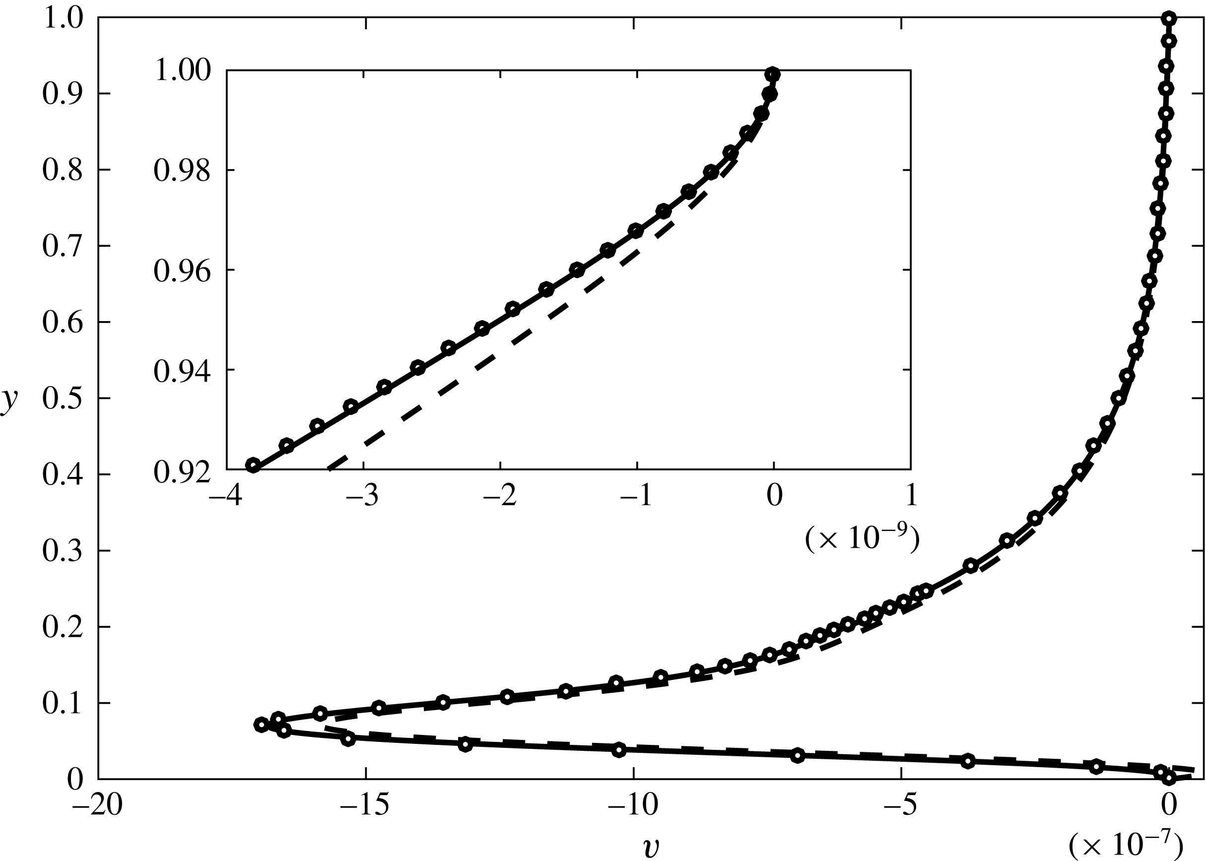
Microfluidic devices are beginning to fulfil their promise in a number of application areas such as in micro total analysis systems (Reyes et al. Reference Reyes, Iossifidis, Auroux and Manz2002), medical diagnostic devices, physical, chemical and biological analytical processes (Song, Chen & Ismagilov Reference Song, Chen and Ismagilov2006; Huebner et al. Reference Huebner, Sharma, Srisa-Art, Hollfelder, Edel and deMello2008; Teh et al. Reference Teh, Lin, Hung and Lee2008) and in mono-sized droplet generation (Baroud, Gallaire & Dangla Reference Baroud, Gallaire and Dangla2010; Anna Reference Anna2016). With such developments, it is important to understand fluid transport or pumping by non-mechanical means, such as capillary, acoustic, electrokinetic and peristaltic mechanisms (Stone, Stroock & Ajdari Reference Stone, Stroock and Ajdari2004; Eldabe et al. Reference Eldabe, El-Sayed, Ghaly and Sayed2007). Laser & Santiago (Reference Laser and Santiago2004) reviewed the development over a 25-year period of micro-scale devices for pumping small amounts of fluids in microfluidic devices.
In this work, we explore an alternative mechanism for non-mechanical pumping of fluid that is well suited when thermal effects are naturally present in microfluidic devices. The mechanism of transporting fluid by density gradients induced by boundary heating has been speculated in the past in a completely different context. In the seventeenth century, Halley (Reference Halley1686) hypothesized that the global atmospheric circulation is caused by the diurnal heating from the Sun as the Earth rotates. Although incorrect, this idea inspired the ‘moving-flame experiment’ by Fultz (Reference Fultz1956), and later by Stern (Reference Stern1959), Schubert & Whitehead (Reference Schubert and Whitehead1969), Douglas, Mason & Hinch (Reference Douglas, Mason and Hinch1972) and Whitehead (Reference Whitehead1972).
In the experiment by Fultz (Reference Fultz1956), a Bunsen flame is rotated beneath a cylindrical container of water. After initial adjustment, a steady surface flow appears opposite to the moving flame direction with magnitude less than one per cent of the flame speed. Stern (Reference Stern1959) used a fixed annulus to restrict the three-dimensional fluid motion and reported similar findings in terms of the surface flow’s direction and speed. The experiment by Schubert & Whitehead (Reference Schubert and Whitehead1969) also uses an annulus, but the working fluid is mercury instead of water. They observed fluid motion opposite to the moving flame with a speed up to four times that of the flame. Whitehead (Reference Whitehead1972) pointed out later that the temperature-dependent surface tension could be partly responsible for this rapid flow. Douglas et al. (Reference Douglas, Mason and Hinch1972) conducted another experiment with mercury to limit the effect of surface tension, and the surface speed reduces to half that of the heat source.
These observations of net horizontal momentum driven by vertical buoyancy forces attracted a lot of theoretical interest. Stern (Reference Stern1959) gave the first theory of this problem. The theory begins with an argument that the only stress that could balance that of the mean flow is the Reynolds stress of velocity fluctuation, induced by the thermal wave. The Boussinesq approximation is made. Instead of solving the heat equation, a temperature distribution of the form
 $A\sin (kx-ct)$
is imposed on the fluid directly. Davey (Reference Davey1967) extended the theory to finite thermal diffusivity and free surfaces. Schubert, Young & Hinch (Reference Schubert, Young and Hinch1971) showed that a thermal wave exerted at the upper free surface could generate horizontal net flow in the same direction as the thermal wave. All these studies have focused on the limiting behaviour of certain parameters, for example, small or large Prandtl number (or viscosity). No attention was given to the maximum induced axial flow possible, which is of interest to engineering optimization. In addition, all previous theories decompose temperature and flow fields into a mean and a fluctuating component (the Reynolds decomposition). Another limitation is the long wave assumption. While it holds for geophysical and astrophysical problems, it usually does not apply in micro-device applications. With these in mind, and considering current computing resources (numerical solvers, computer algebra systems), we feel it is worthwhile to revisit this classic problem and thoroughly explore the parameter space.
In other contexts, Weinert et al. (Reference Weinert, Kraus, Franosch and Braun2008) showed that the nonlinearity caused by thermal expansion and temperature-dependent viscosity could also transport fluid. Mao, Oron & Alexeev (Reference Mao, Oron and Alexeev2013) demonstrated that the travelling spatial modulation of surface tension by heat can transport liquid in thin films. The net flow is driven by spatial variation of surface tension caused by heating, and thus requires an open channel configuration. If the volume expansion by heating is significant, transient heating can be used to transport fluid in the absence of gravity (buoyancy) as revealed by Yariv & Brenner (Reference Yariv and Brenner2004). Compared with above mechanisms, Boussinesq convection is much simpler in driving fluid motion, with no requirement of free surface, varying viscosity or surface tension. The only essential parts are gravitational field in combination with temperature-dependent density causing a variation in the buoyancy force.
Therefore, we are motivated to explore fluid transport inside an enclosed microchannel driven by a travelling temperature wave at the bottom wall. We start with the Navier–Stokes equations with the Boussinesq approximation, together with the convection–diffusion heat equation in § 2. We do not decompose the flow and temperature fields into a mean and a fluctuating component. Instead, the complete flow and temperature fields are solved. The system of equations is shifted to an axial coordinate moving with the travelling temperature wave in § 2.1, and the system becomes steady in the moving frame. A velocity scale
 $V$
is derived by a dominant balance between buoyancy and viscous forces in the vertical momentum equation. The system is made dimensionless by
 $V$
in § 2.2, and four dimensionless groups emerge:
 $Re$
,
 $Rc$
,
 $K$
and
 $Pr$
. Section 3 presents the asymptotic expansion in the limit
 $Re\rightarrow 0$
. The dimensionless induced axial volumetric flow rate
 $Q$
is found analytically to first order in
 $Re$
. A finite-volume numerical method is used to solve the complete system of equations, as described in § 4. Typical flow and temperature fields are presented and compared with the asymptotic solution. Section 5 presents a systematic study of the parameters
 $Re$
,
 $Rc$
,
 $K$
and
 $Pr$
, and their effects on
 $Q$
. The optimal parameters for transport are found in § 6. We discuss some details of this study in § 7 and conclude in § 8.
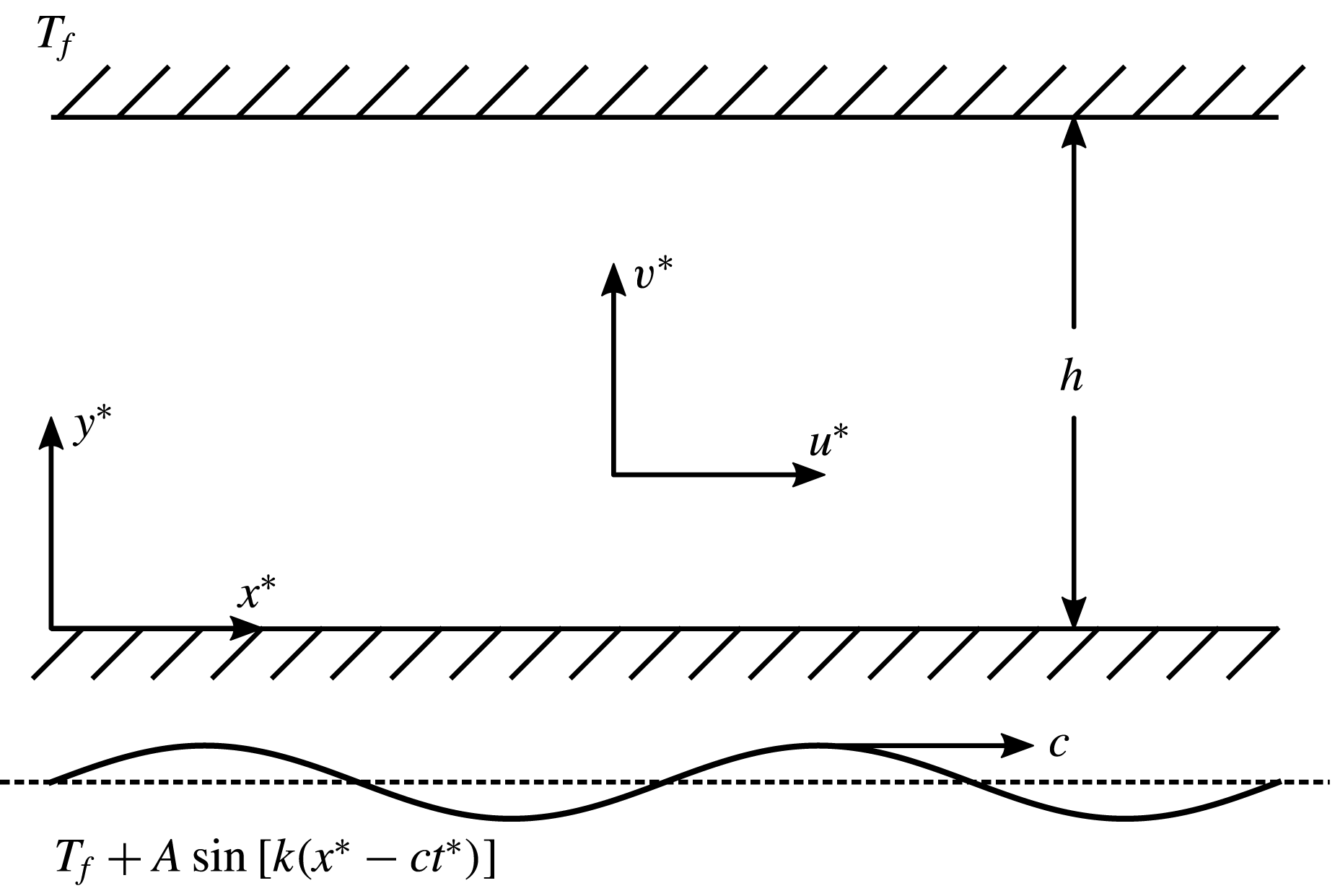
A sketch of the two-dimensional microchannel and the thermal boundary conditions.

2 Mathematical model
2.1 Governing equations in the moving frame
We consider a two-dimensional (2-D) horizontal channel of height
 $h$
, as illustrated in figure 1. A Cartesian coordinate system
 $(x^{\ast },y^{\ast })$
is defined at the bottom wall, with
 $x^{\ast }$
pointing horizontally along the channel and
 $y^{\ast }$
pointing upward. A travelling sinusoidal temperature wave is imposed at the bottom wall. Since the temperature variation is small compared with the mean temperature, we apply the Boussinesq approximation, and the flow and temperature fields obey
 $$\begin{eqnarray}\displaystyle & \displaystyle {\displaystyle \frac{\unicode[STIX]{x2202}\boldsymbol{u}^{\ast }}{\unicode[STIX]{x2202}t^{\ast }}}+\boldsymbol{u}^{\ast }\boldsymbol{\cdot }\unicode[STIX]{x1D735}^{\ast }\boldsymbol{u}^{\ast }=-{\displaystyle \frac{1}{\unicode[STIX]{x1D70C}}}\unicode[STIX]{x1D735}^{\ast }p^{\ast }+\unicode[STIX]{x1D708}\unicode[STIX]{x1D6FB}^{\ast 2}\boldsymbol{u}^{\ast }+\unicode[STIX]{x1D6FD}g\left(T^{\ast }-T_{f}\right)\boldsymbol{j}, & \displaystyle\end{eqnarray}$$
 $$\begin{eqnarray}\displaystyle & \unicode[STIX]{x1D735}^{\ast }\boldsymbol{\cdot }\boldsymbol{u}^{\ast }=0, & \displaystyle\end{eqnarray}$$
 $$\begin{eqnarray}\displaystyle & \displaystyle {\displaystyle \frac{\unicode[STIX]{x2202}T^{\ast }}{\unicode[STIX]{x2202}t^{\ast }}}+\boldsymbol{u}^{\ast }\boldsymbol{\cdot }\unicode[STIX]{x1D735}^{\ast }T^{\ast }=\unicode[STIX]{x1D6FC}\unicode[STIX]{x1D6FB}^{\ast 2}T^{\ast }, & \displaystyle\end{eqnarray}$$
 $$\begin{eqnarray}\displaystyle & \displaystyle \boldsymbol{u}^{\ast }(t^{\ast },x^{\ast },y^{\ast }=0)=\boldsymbol{u}^{\ast }(t^{\ast },x^{\ast },y^{\ast }=h)=0, & \displaystyle\end{eqnarray}$$
 $$\begin{eqnarray}\displaystyle & \displaystyle T^{\ast }(t^{\ast },x^{\ast },y^{\ast }=0)=T_{f}+A\sin [k(x^{\ast }-ct^{\ast })],T^{\ast }(t^{\ast },x^{\ast },y^{\ast }=h)=T_{f}, & \displaystyle\end{eqnarray}$$
 $\unicode[STIX]{x1D735}^{\ast }=\boldsymbol{i}\unicode[STIX]{x2202}/\unicode[STIX]{x2202}x^{\ast }+\boldsymbol{j}\unicode[STIX]{x2202}/\unicode[STIX]{x2202}y^{\ast }$
,
 $\boldsymbol{u}^{\ast }=u^{\ast }\boldsymbol{i}+v^{\ast }\boldsymbol{j}$
is fluid velocity,
 $\unicode[STIX]{x1D70C}$
is density,
 $\unicode[STIX]{x1D708}$
is kinematic viscosity,
 $\unicode[STIX]{x1D6FD}$
is thermal expansion coefficient,
 $g$
is gravitational acceleration,
 $T^{\ast }$
is temperature,
 $\unicode[STIX]{x1D6FC}$
is thermal diffusivity,
 $T_{f}$
is top wall temperature and
 $A$
,
 $k$
and
 $c$
are, respectively, thermal wave amplitude, wavenumber and wave speed. The problem becomes steady in a reference frame moving with the travelling temperature wave. We transform the governing equations to this reference frame by defining
 $x^{\prime }=x^{\ast }-ct^{\ast }$
,
 $y^{\prime }=y^{\ast }$
,
 $t^{\prime }=t^{\ast }$
,
 $u^{\prime }=u^{\ast }$
,
 $v^{\prime }=v^{\ast }$
,
 $p^{\prime }=p^{\ast }$
,
 $T^{\prime }=T^{\ast }$
. The governing equations and boundary conditions are independent of time in the moving frame:
 $$\begin{eqnarray}\displaystyle \left.\begin{array}{@{}c@{}}\displaystyle (\boldsymbol{u}^{\prime }-c\,\boldsymbol{i})\boldsymbol{\cdot }\unicode[STIX]{x1D735}^{\prime }\boldsymbol{u}^{\prime }=-{\displaystyle \frac{1}{\unicode[STIX]{x1D70C}}}\unicode[STIX]{x1D735}^{\prime }p^{\prime }+\unicode[STIX]{x1D708}\unicode[STIX]{x1D6FB}^{\prime 2}\boldsymbol{u}^{\prime }+\unicode[STIX]{x1D6FD}g\left(T^{\prime }-T_{f}\right)\boldsymbol{j},\\[2.0pt] \unicode[STIX]{x1D735}^{\prime }\boldsymbol{\cdot }\boldsymbol{u}^{\prime }=0,\\ (\boldsymbol{u}^{\prime }-c\,\boldsymbol{i})\boldsymbol{\cdot }\unicode[STIX]{x1D735}^{\prime }T^{\prime }=\unicode[STIX]{x1D6FC}\unicode[STIX]{x1D6FB}^{\prime 2}T^{\prime },\\ \boldsymbol{u}^{\prime }(x^{\prime },y^{\prime }=0)=\boldsymbol{u}^{\prime }(x^{\prime },y^{\prime }=h)=0,\\ T^{\prime }(x^{\prime },y^{\prime }=0)=T_{f}+A\sin (kx^{\prime }),T^{\prime }(x^{\prime },y^{\prime }=h)=T_{f},\end{array}\right\} & & \displaystyle\end{eqnarray}$$
where
 $\unicode[STIX]{x1D735}^{\prime }=\boldsymbol{i}\unicode[STIX]{x2202}/\unicode[STIX]{x2202}x^{\prime }+\boldsymbol{j}\unicode[STIX]{x2202}/\unicode[STIX]{x2202}y^{\prime }$
and
 $\boldsymbol{u}^{\prime }=u^{\prime }\boldsymbol{i}+v^{\prime }\boldsymbol{j}$
. By defining
 $\boldsymbol{u}^{\prime }=\boldsymbol{u}^{\ast }$
, we are solving the absolute velocity in the moving reference frame. Consequently, the boundary conditions for
 $\boldsymbol{u}^{\prime }$
remain homogeneous, but the momentum and heat equations gain new convective terms. The solution is periodic in
 $x^{\prime }$
because of the periodic boundary conditions. There are sufficient differential equations and boundary conditions to solve the problem. The induced axial flow rate along the channel can then be found as
 $$\begin{eqnarray}\displaystyle & \displaystyle Q^{\prime }=\int _{0}^{h}u^{\prime }\,\text{d}y^{\prime }. & \displaystyle\end{eqnarray}$$
The main purpose of this paper is to find
 $Q^{\prime }$
.
2.2 Non-dimensionalization
The channel height
 $h$
provides a natural length scale. A dominant balance between the driving buoyancy term and the viscous term in the vertical momentum equation yields a velocity scale:
 $$\begin{eqnarray}\displaystyle & \displaystyle V=\unicode[STIX]{x1D6FD}gAh^{2}/\unicode[STIX]{x1D708}. & \displaystyle\end{eqnarray}$$
Based on these scales, a set of dimensionless variables is defined:
 $$\begin{eqnarray}\displaystyle x={\displaystyle \frac{x^{\prime }}{h}},\quad y={\displaystyle \frac{y^{\prime }}{h}},\quad u={\displaystyle \frac{u^{\prime }}{V}},\quad v={\displaystyle \frac{v^{\prime }}{V}},\quad p={\displaystyle \frac{hp^{\prime }}{\unicode[STIX]{x1D70C}\unicode[STIX]{x1D708}V}},\quad T={\displaystyle \frac{T^{\prime }-T_{f}}{A}},\quad Q={\displaystyle \frac{Q^{\prime }}{Vh}}. & & \displaystyle \nonumber\\ \displaystyle & & \displaystyle\end{eqnarray}$$
The governing equations and boundary conditions are non-dimensionlized:
 $$\begin{eqnarray}\displaystyle & \displaystyle (Re\,\boldsymbol{u}-Rc\,\boldsymbol{i})\boldsymbol{\cdot }\unicode[STIX]{x1D735}\boldsymbol{u}=-\unicode[STIX]{x1D735}p+\unicode[STIX]{x1D6FB}^{2}\boldsymbol{u}+T\boldsymbol{j}, & \displaystyle\end{eqnarray}$$
 $$\begin{eqnarray}\displaystyle & \displaystyle \unicode[STIX]{x1D735}\boldsymbol{\cdot }\boldsymbol{u}=0, & \displaystyle\end{eqnarray}$$
 $$\begin{eqnarray}\displaystyle & \displaystyle (Re\,\boldsymbol{u}-Rc\,\boldsymbol{i})\boldsymbol{\cdot }\unicode[STIX]{x1D735}T=Pr^{-1}\unicode[STIX]{x1D6FB}^{2}T, & \displaystyle\end{eqnarray}$$
 $$\begin{eqnarray}\displaystyle & \displaystyle \boldsymbol{u}(x,y=0)=\boldsymbol{u}(x,y=1)=0, & \displaystyle\end{eqnarray}$$
 $$\begin{eqnarray}\displaystyle & \displaystyle T(x,y=0)=\sin (Kx),T(x,y=1)=0, & \displaystyle\end{eqnarray}$$
 $\unicode[STIX]{x1D735}=\boldsymbol{i}\unicode[STIX]{x2202}/\unicode[STIX]{x2202}x+\boldsymbol{j}\unicode[STIX]{x2202}/\unicode[STIX]{x2202}y$
,
 $\boldsymbol{u}=u\boldsymbol{i}+v\boldsymbol{j}$
,
 $Re=Vh/\unicode[STIX]{x1D708}$
is the Reynolds number based on
 $V$
,
 $Rc=ch/\unicode[STIX]{x1D708}$
is the Reynolds number based on
 $c$
,
 $Pr=\unicode[STIX]{x1D708}/\unicode[STIX]{x1D6FC}$
is the Prandtl number and
 $K=kh$
is the dimensionless thermal wavenumber. The Reynolds number has an identical form to the Grashof number, or the Rayleigh number divided by the Prandtl number. The axial volume flow rate is also made dimensionless:
 $$\begin{eqnarray}\displaystyle & \displaystyle Q=\int _{0}^{1}u\,\text{d}y. & \displaystyle\end{eqnarray}$$
In the next section, we seek a solution in the limit
 $Re\rightarrow 0$
because
 $Re$
is small in microchannels. A full numerical solution will be presented in § 4.
3 Asymptotic solution
In the limit
 $Re\rightarrow 0$
, the dependent variables are expanded in asymptotic series as
 $$\begin{eqnarray}\displaystyle \left.\begin{array}{@{}l@{}}\boldsymbol{u}=\boldsymbol{u}_{\mathbf{0}}+Re\,\boldsymbol{u}_{\mathbf{1}}+\cdots \,,\\ p=p_{0}+Re\,p_{1}+\cdots \,,\\ T=T_{0}+Re\,T_{1}+\cdots \,,\end{array}\right\} & & \displaystyle\end{eqnarray}$$
where
 $\boldsymbol{u}_{\mathbf{0}}=u_{0}\boldsymbol{i}+v_{0}\boldsymbol{j}$
and
 $\boldsymbol{u}_{\mathbf{1}}=u_{1}\boldsymbol{i}+v_{1}\boldsymbol{j}$
. The induced axial volume flow rate is also expanded as
 $$\begin{eqnarray}\displaystyle & \displaystyle Q=Q_{0}+ReQ_{1}+\cdots \,, & \displaystyle\end{eqnarray}$$
 $$\begin{eqnarray}\displaystyle & \displaystyle Q_{0}=\int _{0}^{1}u_{0}\,\text{d}y,\quad Q_{1}=\int _{0}^{1}u_{1}\,\text{d}y. & \displaystyle\end{eqnarray}$$
3.1 Leading order
At the leading order, the governing equations and boundary conditions are
 $$\begin{eqnarray}\displaystyle \left.\begin{array}{@{}c@{}}\displaystyle -Rc{\displaystyle \frac{\unicode[STIX]{x2202}\boldsymbol{u}_{\mathbf{0}}}{\unicode[STIX]{x2202}x}}=-\unicode[STIX]{x1D735}p_{0}+\unicode[STIX]{x1D735}^{2}\boldsymbol{u}_{\boldsymbol{ 0}}+T_{0}\,\boldsymbol{j},\\[8.0pt] \displaystyle \unicode[STIX]{x1D735}\boldsymbol{\cdot }\boldsymbol{u}_{\mathbf{0}}=0,\\[8.0pt] \displaystyle -Rc{\displaystyle \frac{\unicode[STIX]{x2202}T_{0}}{\unicode[STIX]{x2202}x}}=Pr^{-1}\unicode[STIX]{x1D6FB}^{2}T_{0},\\[8.0pt] \displaystyle \boldsymbol{u}_{\mathbf{0}}(x,0)=\boldsymbol{u}_{\mathbf{0}}(x,1)=0,\quad T_{0}(x,0)=\sin (Kx),\quad T_{0}(x,1)=0.\end{array}\right\} & & \displaystyle\end{eqnarray}$$
The pressure term is then eliminated from the momentum equation by cross-differentiation. The horizontal velocity
 $u_{0}$
is eliminated from the combined momentum equation using the continuity equation, and we are left with
 $$\begin{eqnarray}\displaystyle \left.\begin{array}{@{}c@{}}\displaystyle Rc\unicode[STIX]{x1D6FB}^{2}{\displaystyle \frac{\unicode[STIX]{x2202}v_{0}}{\unicode[STIX]{x2202}x}}+\unicode[STIX]{x1D6FB}^{4}v_{0}+{\displaystyle \frac{\unicode[STIX]{x2202}^{2}T_{0}}{\unicode[STIX]{x2202}x^{2}}}=0,\\[8.0pt] \displaystyle Rc{\displaystyle \frac{\unicode[STIX]{x2202}T_{0}}{\unicode[STIX]{x2202}x}}+Pr^{-1}\unicode[STIX]{x1D6FB}^{2}T_{0}=0,\\[8.0pt] \displaystyle v_{0}(x,0)=v_{0}(x,1)={\displaystyle \frac{\unicode[STIX]{x2202}v_{0}}{\unicode[STIX]{x2202}y}}(x,0)={\displaystyle \frac{\unicode[STIX]{x2202}v_{0}}{\unicode[STIX]{x2202}y}}(x,1)=0,\\[8.0pt] T_{0}(x,0)=\sin (Kx),\quad T_{0}(x,1)=0.\end{array}\right\} & & \displaystyle\end{eqnarray}$$
Since the thermal boundary condition is periodic in
 $x$
, we take
 $$\begin{eqnarray}\displaystyle & \displaystyle v_{0}=\text{Im}[F(y)\text{e}^{\text{i}Kx}], & \displaystyle\end{eqnarray}$$
 $$\begin{eqnarray}\displaystyle & \displaystyle T_{0}=\text{Im}[G(y)\text{e}^{\text{i}Kx}], & \displaystyle\end{eqnarray}$$
 $\text{Im}$
stands for the imaginary part. Substitution of these into (3.4) yields a pair of coupled linear ordinary differential equations:
 $$\begin{eqnarray}\displaystyle & \displaystyle {\displaystyle \frac{\text{d}^{4}F}{\text{d}y^{4}}}+(\text{i}RcK-2K^{2}){\displaystyle \frac{\text{d}^{2}F}{\text{d}y^{2}}}-K^{2}(\text{i}RcK-K^{2})F=K^{2}G, & \displaystyle\end{eqnarray}$$
 $$\begin{eqnarray}\displaystyle & \displaystyle {\displaystyle \frac{\text{d}^{2}G}{\text{d}y^{2}}}+(\text{i}RcKPr-K^{2})G=0, & \displaystyle\end{eqnarray}$$
 $$\begin{eqnarray}\displaystyle & \displaystyle F(0)=F(1)={\displaystyle \frac{\text{d}F}{\text{d}y}}(0)={\displaystyle \frac{\text{d}F}{\text{d}y}}(1)=0, & \displaystyle\end{eqnarray}$$
 $$\begin{eqnarray}\displaystyle & \displaystyle G(0)=1,G(1)=0. & \displaystyle\end{eqnarray}$$
 $$\begin{eqnarray}\displaystyle & \displaystyle G(y)={\displaystyle \frac{\sin [\sqrt{\text{i}RcKPr-K^{2}}(1-y)]}{\sin [\sqrt{\text{i}RcKPr-K^{2}}]}}. & \displaystyle\end{eqnarray}$$
Equation (3.6a
) then yields an analytic solution for
 $F(y)$
, which is listed in appendix A because of its length. The horizontal velocity
 $u_{0}$
is found from
 $v_{0}$
as
 $$\begin{eqnarray}\displaystyle & \displaystyle u_{0}=\text{Im}\left[{\displaystyle \frac{\text{i}}{K}}{\displaystyle \frac{\text{d}F}{\text{d}y}}\text{e}^{\text{i}Kx}\right]. & \displaystyle\end{eqnarray}$$
Thus, the leading-order volume flow rate is found to be zero:
 $$\begin{eqnarray}\displaystyle & \displaystyle Q_{0}=\int _{0}^{1}u_{0}\,\text{d}y=0. & \displaystyle\end{eqnarray}$$
3.2 First order
The first-order governing equations and boundary conditions are
 $$\begin{eqnarray}\displaystyle & \displaystyle -\unicode[STIX]{x1D735}p_{1}+\unicode[STIX]{x1D6FB}^{2}\boldsymbol{u}_{\mathbf{1}}+T_{1}\,\boldsymbol{j}+Rc{\displaystyle \frac{\unicode[STIX]{x2202}\boldsymbol{u}_{\mathbf{1}}}{\unicode[STIX]{x2202}x}}=\boldsymbol{u}_{\mathbf{0}}\boldsymbol{\cdot }\unicode[STIX]{x1D735}\boldsymbol{u}_{\mathbf{0}}, & \displaystyle\end{eqnarray}$$
 $$\begin{eqnarray}\displaystyle & \displaystyle \unicode[STIX]{x1D735}\boldsymbol{\cdot }\boldsymbol{u}_{\mathbf{1}}=0, & \displaystyle\end{eqnarray}$$
 $$\begin{eqnarray}\displaystyle & \displaystyle {\displaystyle \frac{1}{Pr}}\unicode[STIX]{x1D6FB}^{2}T_{1}+Rc{\displaystyle \frac{\unicode[STIX]{x2202}T_{1}}{\unicode[STIX]{x2202}x}}=\boldsymbol{u}_{\mathbf{0}}\boldsymbol{\cdot }\unicode[STIX]{x1D735}T_{0}, & \displaystyle\end{eqnarray}$$
 $$\begin{eqnarray}\displaystyle & \displaystyle \boldsymbol{u}_{\mathbf{1}}(x,0)=\boldsymbol{u}_{\mathbf{1}}(x,1)=T_{1}(x,0)=T_{1}(x,1)=0. & \displaystyle\end{eqnarray}$$
 $Q$
, we only need to focus on the horizontal velocity component
 $u_{1}$
, which obeys
 $$\begin{eqnarray}\displaystyle & \displaystyle -{\displaystyle \frac{\unicode[STIX]{x2202}p_{1}}{\unicode[STIX]{x2202}x}}+{\displaystyle \frac{\unicode[STIX]{x2202}^{2}u_{1}}{\unicode[STIX]{x2202}x^{2}}}+{\displaystyle \frac{\unicode[STIX]{x2202}^{2}u_{1}}{\unicode[STIX]{x2202}y^{2}}}+Rc{\displaystyle \frac{\unicode[STIX]{x2202}u_{1}}{\unicode[STIX]{x2202}x}}=u_{0}{\displaystyle \frac{\unicode[STIX]{x2202}u_{0}}{\unicode[STIX]{x2202}x}}+v_{0}{\displaystyle \frac{\unicode[STIX]{x2202}u_{0}}{\unicode[STIX]{x2202}y}}. & \displaystyle\end{eqnarray}$$
Averaging (3.11) in the
 $x$
direction over the thermal wavelength
 $2\unicode[STIX]{x03C0}/K$
yields
 $$\begin{eqnarray}\displaystyle & \displaystyle {\displaystyle \frac{\text{d}^{2}\overline{u}_{1}}{\text{d}y^{2}}}={\displaystyle \frac{\text{d}\overline{u_{0}v_{0}}}{\text{d}y}}, & \displaystyle\end{eqnarray}$$
where the overline means horizontal average over the thermal wavelength. All other terms vanish owing to periodicity in
 $x$
. The equation states that the averaged horizontal viscous shear stress is balanced by the Reynolds stress. Solving (3.12) together with the boundary conditions
 $\overline{u}_{1}(0)=\overline{u}_{1}(1)=0$
gives
 $$\begin{eqnarray}\displaystyle & \displaystyle \overline{u}_{1}(y)=\int _{0}^{y}\overline{u_{0}v_{0}}\,\text{d}\unicode[STIX]{x1D709}-y\int _{0}^{1}\overline{u_{0}v_{0}}\,\text{d}\unicode[STIX]{x1D709}=\int _{0}^{y}\left(\overline{u_{0}v_{0}}-\langle \overline{u_{0}v_{0}}\rangle \right)\,\text{d}\unicode[STIX]{x1D709}. & \displaystyle\end{eqnarray}$$
The angle brackets denote vertical average over the entire interval
 $[0,1]$
, so this term is a constant. The first-order volume flow rate
 $Q_{1}$
is found as
 $$\begin{eqnarray}\displaystyle & \displaystyle Q_{1}=\int _{0}^{1}\overline{u}_{1}(y)\,\text{d}y=\int _{0}^{1}\int _{0}^{y}\left(\overline{u_{0}v_{0}}-\langle \overline{u_{0}v_{0}}\rangle \right)\,\text{d}\unicode[STIX]{x1D709}\,\text{d}y. & \displaystyle\end{eqnarray}$$
If
 $F(y)$
is decomposed into real and imaginary parts as
 $F_{R}(y)+\text{i}F_{I}(y)$
,
 $v_{0}$
and
 $u_{0}$
can be found by substituting it into (3.5a
) and (3.8), respectively. Then, the Reynolds stress is found as
 $$\begin{eqnarray}\displaystyle & \displaystyle \overline{u_{0}v_{0}}={\displaystyle \frac{1}{2K}}\left(F_{I}{\displaystyle \frac{\text{d}F_{R}}{\text{d}y}}-F_{R}{\displaystyle \frac{\text{d}F_{I}}{\text{d}y}}\right). & \displaystyle\end{eqnarray}$$
The integrals in (3.14) are evaluated numerically to an accuracy of seven significant digits (appendix B). Thus, the volume flow rate
 $Q$
is
 $$\begin{eqnarray}\displaystyle Q(Re,Rc,Pr,K)=ReQ_{1}(Rc,Pr,K). & & \displaystyle\end{eqnarray}$$
This concludes the asymptotic solution of the volume flow rate. In the next section, we present the numerical method used to solve (2.6), and two typical solutions.
4 Numerical method and typical solutions
We use the finite-volume computational-fluid-dynamics (CFD) toolkit OpenFOAM (Jasak, Jemcov & Tukovic Reference Jasak, Jemcov and Tukovic2007) to solve (2.6). Our solver is based on the buoyantBoussinesqPimpleFoam solver distributed with OpenFOAM version 3.0. We treat the problem as a transient one and use time marching to reach the steady state. The PIMPLE algorithm, which is a combination of the SIMPLE (semi-implicit method for pressure-linked equations) algorithm and the PISO (pressure-implicit split-operator) algorithm, is used to iteratively resolve the incompressibility constraint. To add the extra convective term in (2.6), we adapt the approach used by OpenFOAM (and many other CFD codes) to handle a moving reference frame or dynamic mesh motion; the face-based flux field is temporarily changed to include the extra convective term, then it is changed back before solving for the pressure constraint. All the customizations of the solver have been validated before applying to this problem; validation cases include linear convection, pressure distribution in a stable Rayleigh–Bénard set-up, critical Rayleigh number for the Rayleigh instability and several mesh-independence studies to verify the second-order spatial and temporal accuracy (Zhang Reference Zhang2017).
The system (2.6) is solved for
 $K=2\unicode[STIX]{x03C0}$
,
 $Pr=1$
and five
 $Rc$
values, each with fifteen different
 $Re$
values. A mesh is created which is uniform in
 $x$
(64 cells), and has a gentle gradation in
 $y$
(128 cells). The gradation is introduced such that the mesh better resolves the bottom wall boundary layer. Time marching starts from the initial state of uniform temperature and pressure, and zero velocity. The solution is considered converged when the absolute change of the maximum velocity magnitude is less than
 $10^{-16}$
. A mesh-independence study shows that the solutions obtained in this way have at least three significant digits.
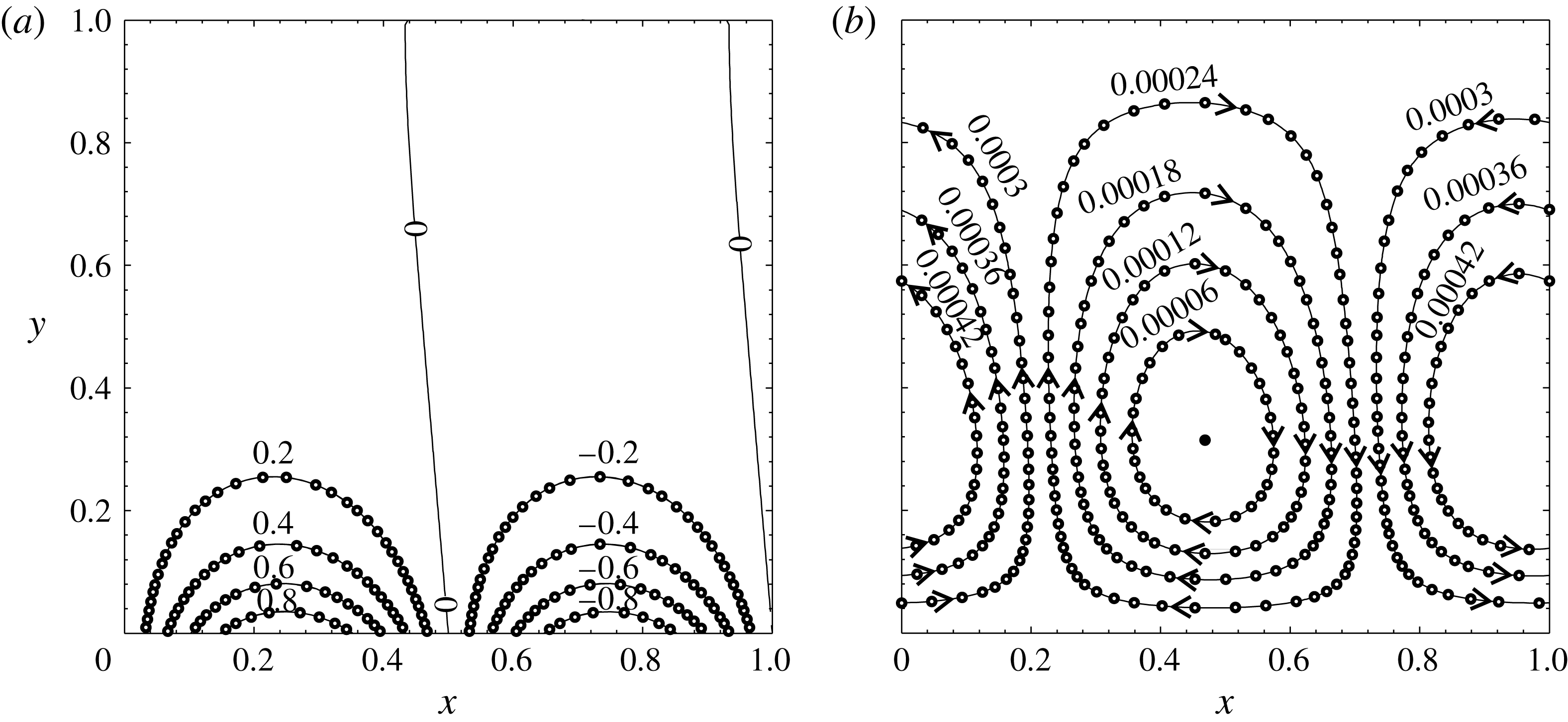
Contour plots of temperature
 $T$
(a) and streamfunction
 $\unicode[STIX]{x1D6F9}$
(b) for
 $Re=Rc=Pr=1$
and
 $K=2\unicode[STIX]{x03C0}$
. The solid lines are analytic leading-order asymptotic solutions, and the open circles are numerical solutions calculated using OpenFOAM.

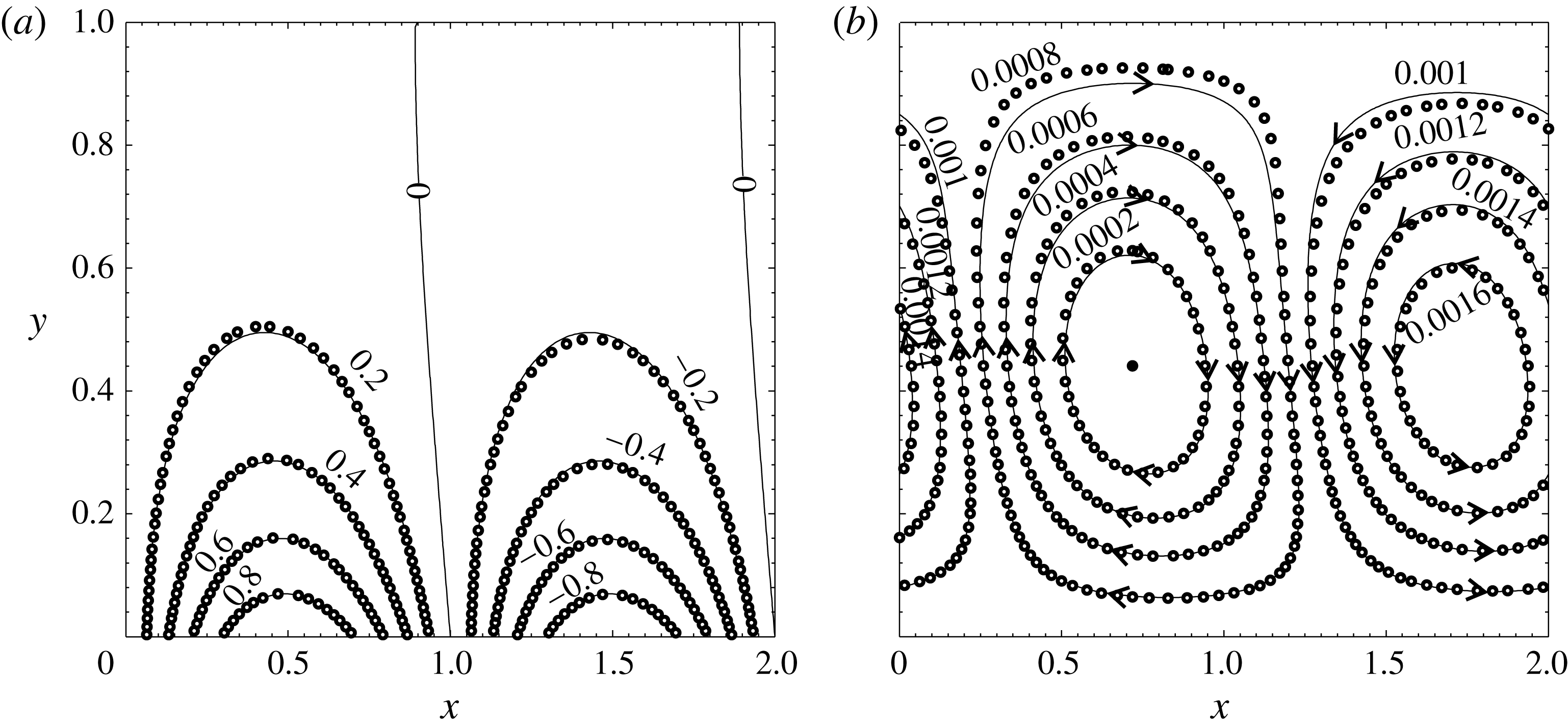
Contour plots of temperature
 $T$
(a) and streamfunction
 $\unicode[STIX]{x1D6F9}$
(b) for
 $Re=1000$
,
 $Rc=10$
,
 $K=\unicode[STIX]{x03C0}$
and
 $Pr=0.1$
. The solid lines are analytic leading-order asymptotic solutions, and the open circles are numerical solutions computed using OpenFOAM. Note the
 $x$
range is different from that in figure 2.

Figure 2 presents a typical solution of the temperature and flow fields for
 $Re=1$
. The leading-order asymptotic solutions are also plotted (solid lines). The flow field is shown through the streamfunction
 $\unicode[STIX]{x1D6F9}$
. For the analytic asymptotic solutions,
 $\unicode[STIX]{x1D6F9}$
is calculated as follows. After
 $v_{0}$
is obtained with the formula in appendix A,
 $u_{0}$
is calculated numerically using finite differences. With
 $u_{0}$
and
 $v_{0}$
known,
 $\unicode[STIX]{x1D6F9}_{0}$
is integrated by Simpson’s rule. The asymptotic and numerical solutions agree well with relative error of approximated
 $0.1\,\%$
. When
 $Re$
is increased, the asymptotic solution starts to deviate from the numerical solution. Figure 3 shows such a case for
 $Re=1000$
. Note that
 $Pr$
and
 $K$
are changed as well to explore the asymptotic solutions’ applicability. Regarding the temperature contours, the asymptotic solution gives the same contour shapes over the hot and code regions, whereas the numerical solution displaces slightly upward over the hot region and downward over the cold region. The streamlines undergo similar changes; the convection cell rises over the hot region, and sinks over the cold region. These changes suggest stronger velocity–temperature coupling, and stronger nonlinear effects. The relative error between the numerical and asymptotic results in figure 3 is approximately
 $2\,\%$
. It is worth pointing out that the temperature profiles in figures 2 and 3 are similar even though the thermal wave speed in figure 3 is ten times faster. The effect of high wave speed is cancelled by the tenfold increase of the thermal diffusivity (
 $Pr$
is reduced by ten times).
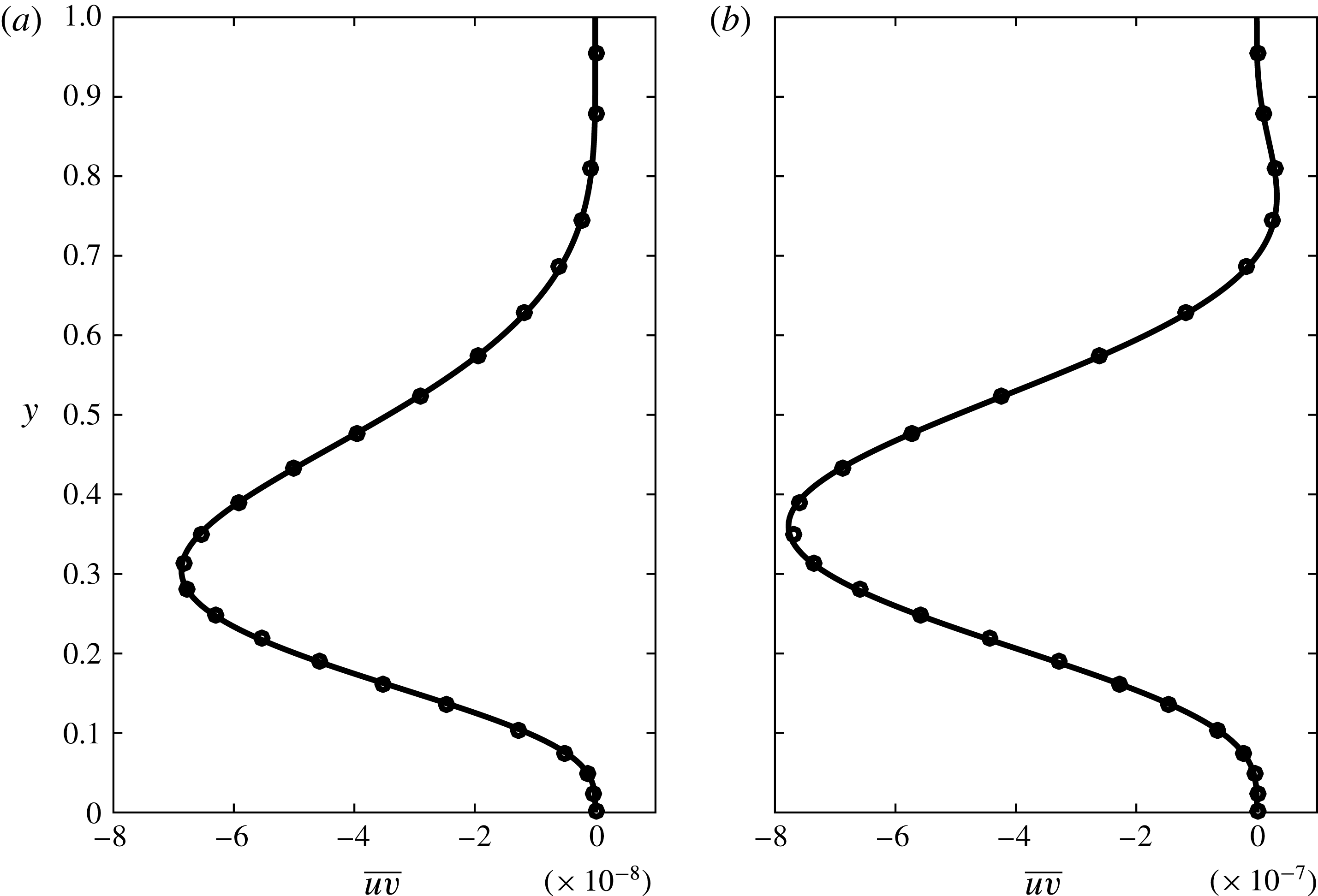
Since the flow is driven by the Reynolds stress, we plot
 $\overline{uv}$
in figure 4 for the cases considered in figures 2 and 3. The numerical solution is obtained by averaging the product of the
 $u$
and
 $v$
velocity fields of the OpenFOAM solution. The asymptotic solution of
 $\overline{u_{0}v_{0}}$
is found from (3.15). Figure 4 shows that the Reynolds stress is mostly negative in the middle region of the channel, which is responsible for the volume flow rate in the
 $-x$
direction. The Reynolds stress
 $\overline{uv}$
, its gradient and its curvature all vanish at the wall owing to the no-slip boundary condition.


5 Effects of model parameters on
 $Q$

From the OpenFOAM solution,
 $Q$
is calculated as the sum of the volume flow rates across the discretized right domain boundary. The numerical value of
 $Q$
has at least three significant digits, the same as that of the flow field.
5.1 Reynolds number
$Re$

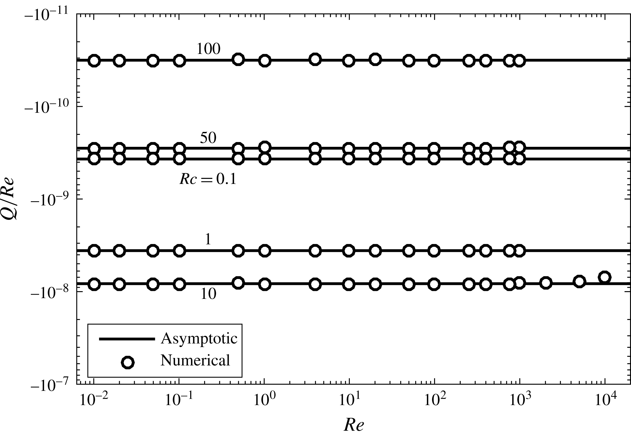
The asymptotic solution in (3.16) gives
 $Q=ReQ_{1}(Rc,Pr,K)$
. Thus
 $Q/Re$
is plotted against
 $Re$
in figure 5 for
 $Pr=1$
,
 $K=2\unicode[STIX]{x03C0}$
and various
 $Rc$
. We expect that the numerical solutions would agree with the asymptotic predictions at
 $Re\ll 1$
, and the two would diverge starting at
 $Re\sim 1$
. Surprisingly, the two maintain agreement all the way to
 $Re=1000$
for all
 $Rc$
cases studied. We also try other
 $Pr$
and
 $K$
values and observe the same agreement. This is unexpected, especially considering that the velocity fields already start to separate at
 $Re=1000$
in figure 3. We compute the
 $Rc=10$
case for
 $Re>10^{3}$
, and find that the asymptotic prediction begins to deviate from the numerical solution at
 $Re=10^{4}$
. We double and redouble the mesh resolutions and conclude that the
 $Q$
values for these three high
 $Re$
cases are accurate to at least six significant digits. Thus, the deviation is physical and not caused by numerical errors. Similar deviations are observed for other
 $Pr$
and
 $K$
values.
Ratio of volume flow rate
 $Q$
to
 $Re$
versus
 $Re$
for
 $K=2\unicode[STIX]{x03C0}$
,
 $Pr=1$
and various
 $Rc$
values. The
 $Rc=10$
case is pushed to extra high
 $Re$
to show the divergence of the numerical and asymptotic solutions.

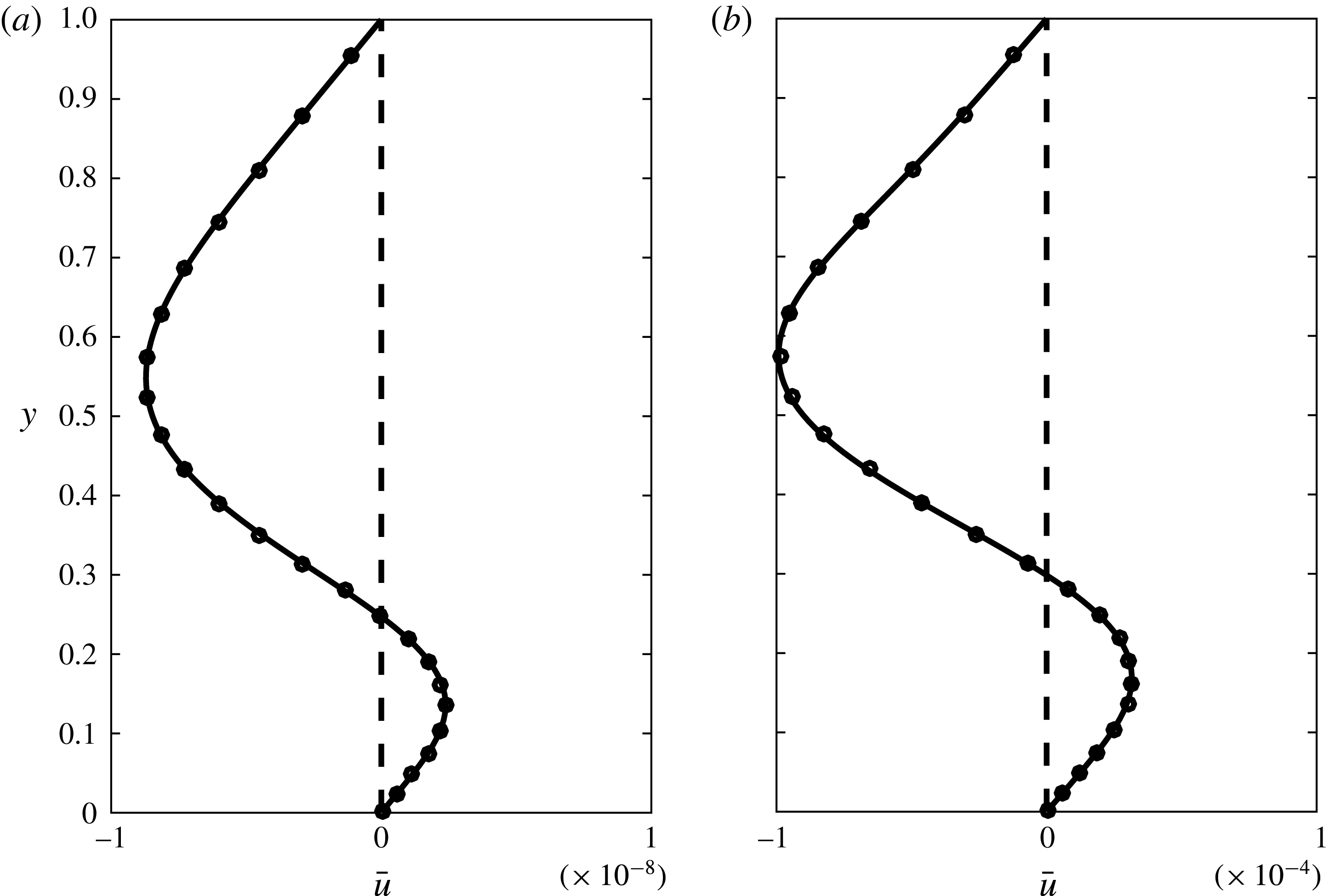
The horizontally averaged velocity
 $\bar{u}(y)$
is studied for
 $Re=1$
and
 $1000$
. Since
 $Q$
is calculated by a vertical integration of
 $\bar{u}(y)$
, the numerical and asymptotic solutions of
 $\bar{u}(y)$
will help to explain why the two solutions of
 $Q$
agree well at
 $Re=10^{4}$
, whereas those of the velocity field start to deviate at
 $Re=10^{3}$
. The velocity
 $\bar{u}(y)$
is found by averaging
 $u(x,y)$
over the wavelength
 $2\unicode[STIX]{x03C0}/K$
in the horizontal direction. Figure 6 shows
 $\bar{u}(y)$
for the two cases studied in figures 2 (
 $Re=1$
) and 3 (
 $Re=1000$
). The leading-order asymptotic solution
 $u_{0}(x,y)$
in (3.8) consists of simple
 $\sin (x)$
and
 $\cos (x)$
functions and averages to zero. The first-order solution
 $u_{1}(x,y)$
contains
 $\sin ^{2}(x)$
and
 $\cos ^{2}(x)$
terms and averages to non-zero. The good agreement between
 $Re\,\bar{u}_{1}(y)$
and the numerical solution for
 $Re=1000$
shows that the differences between the velocity fields in figure 3 mostly cancel themselves when averaged. Since
 $Q$
is the vertical integration of
 $\bar{u}(y)$
, and can be considered as an average of an average, the asymptotic solution of
 $Q$
is accurate at much higher
 $Re$
than that of
 $\boldsymbol{u}_{0}$
.
The horizontally averaged velocity profile
 $\bar{u}(y)$
. The cases in figures 2 and 3 are plotted in (a) and (b), respectively. Shown in each panel are the numerical solution (open circles), the leading-order asymptotic solution
 $\bar{u}_{0}$
(dashed line) and the first-order solution
 $Re\,\bar{u}_{1}$
(solid line).

Since
 $Re$
is not high for flow in microchannels, we study
 $Q$
only for
 $Re\leqslant 10^{3}$
, and rely solely on the asymptotic solution
 $Q_{1}$
to explore the effects of other parameters (
 $Rc$
,
 $K$
and
 $Pr$
).
5.2 Reynolds number
$Rc$
based on the wave speed

Figure 5 shows that
 $Q$
varies non-monotonically with
 $Rc$
;
 $|Q|$
increases then decreases with
 $Rc$
, and vanishes in the small and large
 $Rc$
limits. The limiting behaviour can be understood as follows. When
 $Rc=0$
, the flow consists of convection cells that span across the channel and therefore
 $Q=0$
; when
 $Rc\rightarrow \infty$
, both flow velocity and
 $Q$
vanish owing to the fast alternation of heating and cooling at the bottom wall. The asymptotic solutions of
 $Q_{1}$
in the limits
 $Rc\rightarrow 0$
and
 $\infty$
are derived next.
5.2.1 Asymptotic solution of
$Q_{1}$
in the limit
$Rc\rightarrow 0$


Instead of expanding the complex solution of
 $F(y)$
in appendix A, we find it more revealing to start from the governing equation (3.6a
), and expand
 $F$
in an asymptotic series in
 $Rc$
:
 $$\begin{eqnarray}\displaystyle F(y)=F_{0}(y)+RcF_{1}(y)+\cdots \,. & & \displaystyle\end{eqnarray}$$
The solution of
 $G(y)$
in (3.7) is expanded in the limit
 $Rc\rightarrow 0$
as
 $$\begin{eqnarray}\displaystyle G(y) & = & \displaystyle \text{csch}(K)\sinh [K(1-y)]\nonumber\\ \displaystyle & & \displaystyle +\,{\textstyle \frac{1}{4}}\text{i}PrRc\,\text{csch}^{2}(K)\{(y-2)\sinh (Ky)-y\sinh [K(y-2)]\}+O(Rc^{2}).\end{eqnarray}$$
Note that the leading-order term of
 $G(y)$
is non-zero which is responsible for generating convection cells when
 $Rc=0$
, but it cannot generate axial flow in the channel. When (5.1) and (5.2) are substituted into (3.6a,c
), we obtain
 $$\begin{eqnarray}\displaystyle & & \displaystyle \displaystyle {\displaystyle \frac{\text{d}^{4}F_{0}}{\text{d}y^{4}}}-2K^{2}{\displaystyle \frac{\text{d}^{2}F_{0}}{\text{d}y^{2}}}+K^{4}F_{0}=K^{2}\text{csch}(K)\sinh [K(1-y)],\end{eqnarray}$$
 $$\begin{eqnarray}\displaystyle & & \displaystyle \displaystyle {\displaystyle \frac{\text{d}^{4}F_{1}}{\text{d}y^{4}}}-2K^{2}{\displaystyle \frac{\text{d}^{2}F_{1}}{\text{d}y^{2}}}+K^{4}F_{1}=-\text{i}K{\displaystyle \frac{\text{d}^{2}F_{0}}{\text{d}y^{2}}}+\text{i}K^{3}F_{0}\nonumber\\ \displaystyle & & \displaystyle \quad \displaystyle +\,\frac{1}{4}\text{i}K^{2}Pr\,\text{csch}^{2}(K)\{(y-2)\sinh (Ky)-y\sinh [K(y-2)]\},\end{eqnarray}$$
 $$\begin{eqnarray}\displaystyle & & \displaystyle \displaystyle F_{i}(0)=F_{i}(1)={\displaystyle \frac{\text{d}F_{i}}{\text{d}y}}(0)={\displaystyle \frac{\text{d}F_{i}}{\text{d}y}}(1)=0\quad \text{for}~i=0,1.\end{eqnarray}$$
 $F_{0}$
has a real solution. Thus,
 $F_{1}$
has a pure imaginary solution, according to (5.3b
). These solutions are readily obtained with any computer algebra system, and omitted here due to their length. Substitution of
 $F$
in (5.1) into (3.15) gives
 $$\begin{eqnarray}\displaystyle & \displaystyle \overline{u_{0}v_{0}}={\displaystyle \frac{Rc}{2\text{i}K}}\left({\displaystyle \frac{\text{d}F_{0}}{\text{d}y}}F_{1}-F_{0}{\displaystyle \frac{\text{d}F_{1}}{\text{d}y}}\right)+O(Rc^{2}). & \displaystyle\end{eqnarray}$$
The first-order volume flow rate is then calculated from (3.14):
 $$\begin{eqnarray}\displaystyle \displaystyle Q_{1} & = & \displaystyle -{\displaystyle \frac{(1+Pr)Rc}{645120K^{7}\left(\text{e}^{2K}-1\right)^{2}\left[(\text{e}^{2K}-1)^{2}-4K^{2}\text{e}^{2K}\right]}}\left\{315\left[\text{e}^{8K}(K-5)+K+5\right]\right.\nonumber\\ \displaystyle & & \displaystyle +\,2\text{e}^{6K}\left(12K^{7}+70K^{6}-420K^{5}+2520K^{4}-3360K^{3}+3150K^{2}+2520K+1575\right)\nonumber\\ \displaystyle & & \displaystyle +\,2\text{e}^{4K}\left(8K^{9}+256K^{7}+1680K^{5}-5880K^{3}-5355K\right)+2\text{e}^{2K}\left(12K^{7}-70K^{6}\right.\nonumber\\ \displaystyle & & \displaystyle \left.\!\left.-\,420K^{5}-2520K^{4}-3360K^{3}-3150K^{2}+2520K-1575\right)\!\right\}.\end{eqnarray}$$
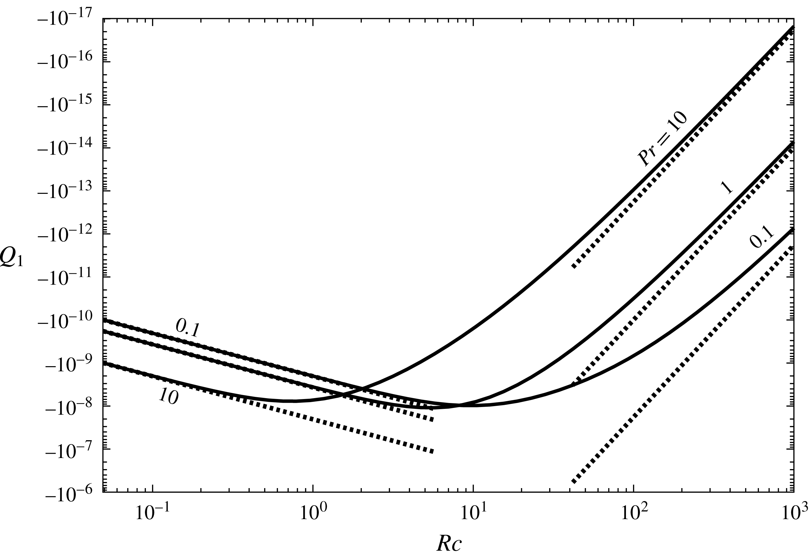
This is plotted in figure 7 and agrees with the full asymptotic solution when
 $Rc$
is small.
First-order asymptotic flow rate
 $Q_{1}$
versus
 $Rc$
for
 $K=2\unicode[STIX]{x03C0}$
and various
 $Pr$
. The solid lines are the full solution of
 $Q_{1}$
calculated by the method described in appendix B. The dashed lines are the small and large
 $Rc$
asymptotic solutions (5.5) and (5.14), respectively.

5.2.2 Asymptotic solution of
$Q_{1}$
in the limit
$Rc\rightarrow \infty$


Equation (3.6a
) is singular in this limit. The solution is expected to have a boundary layer at the bottom wall because as the wave speed increases, the heating and cooling by the wave at the bottom wall will cancel away from the wall. A dominant balance between the first and second terms of (3.6a
) suggests that the boundary-layer thickness scales as
 $1/\sqrt{Rc}$
. Thus, we define a small parameter
 $\unicode[STIX]{x1D716}=1/\sqrt{Rc}$
, and (3.6a
) becomes
 $$\begin{eqnarray}\displaystyle \displaystyle \unicode[STIX]{x1D716}^{2}{\displaystyle \frac{\text{d}^{4}F}{\text{d}y^{4}}}+K(\text{i}-2K\unicode[STIX]{x1D716}^{2}){\displaystyle \frac{\text{d}^{2}F}{\text{d}y^{2}}}-K^{3}(\text{i}-K\unicode[STIX]{x1D716}^{2})F=\unicode[STIX]{x1D716}^{2}K^{2}G(y). & & \displaystyle\end{eqnarray}$$
Equation (5.6) is singular in the limit
 $\unicode[STIX]{x1D716}\rightarrow 0$
, and is solved by the method of matched asymptotic expansions.
In the outer region,
 $G(y)$
expands to
 $\text{e}^{-(1-\text{i})\sqrt{KPr/2}\,y/\unicode[STIX]{x1D716}}$
, which is exponentially small in the limit
 $\unicode[STIX]{x1D716}\rightarrow 0$
and can be safely dropped. Substituting
 $F=F_{0}(y)+\unicode[STIX]{x1D716}F_{1}(y)+\unicode[STIX]{x1D716}^{2}F_{2}(y)+\unicode[STIX]{x1D716}^{3}F_{3}(y)+\unicode[STIX]{x1D716}^{4}F_{4}(y)+\cdots \,$
into (5.6), we find
 $$\begin{eqnarray}\displaystyle \left.\begin{array}{@{}c@{}}\displaystyle {\displaystyle \frac{\text{d}^{2}F_{0}}{\text{d}y^{2}}}-K^{2}F_{0}=0,\\[10.0pt] \displaystyle {\displaystyle \frac{\text{d}^{2}F_{1}}{\text{d}y^{2}}}-K^{2}F_{1}=0,\\[7.0pt] \displaystyle {\displaystyle \frac{\text{d}^{2}F_{2}}{\text{d}y^{2}}}-K^{2}F_{2}={\displaystyle \frac{\text{i}}{K}}\frac{\text{d}^{4}F_{0}}{\text{d}y^{4}}-2\text{i}K\frac{\text{d}^{2}F_{0}}{\text{d}y^{2}}+\text{i}K^{3}F_{0},\\[10.0pt] \displaystyle {\displaystyle \frac{\text{d}^{2}F_{3}}{\text{d}y^{2}}}-K^{2}F_{3}={\displaystyle \frac{\text{i}}{K}}\frac{\text{d}^{4}F_{1}}{\text{d}y^{4}}-2\text{i}K\frac{\text{d}^{2}F_{1}}{\text{d}y^{2}}+\text{i}K^{3}F_{1},\\[10.0pt] \displaystyle {\displaystyle \frac{\text{d}^{2}F_{4}}{\text{d}y^{2}}}-K^{2}F_{4}={\displaystyle \frac{\text{i}}{K}}\frac{\text{d}^{4}F_{2}}{\text{d}y^{4}}-2\text{i}K\frac{\text{d}^{2}F_{2}}{\text{d}y^{2}}+\text{i}K^{3}F_{2}.\end{array}\right\} & & \displaystyle\end{eqnarray}$$
Thus, the fourth-order ordinary differential equation (5.6) has been reduced by two orders, and only two boundary conditions are needed. We apply the no-penetration condition at the top wall:
 $$\begin{eqnarray}\displaystyle \displaystyle F_{i}(1)=0\quad \text{for}~i=0,1,2,3,\ldots . & & \displaystyle\end{eqnarray}$$
The other boundary condition will come from matching with the inner solution. We find
 $F_{0}=F_{1}=F_{2}=F_{3}=0$
because their corresponding inner solutions are zero (see below). Thus,
 $$\begin{eqnarray}\displaystyle & \displaystyle F_{4}=C\text{e}^{-ky}\left(\text{e}^{2ky}-\text{e}^{2k}\right), & \displaystyle\end{eqnarray}$$
where
 $C$
is an integration constant to be determined by matching.
In the inner region, we define
 $\unicode[STIX]{x1D702}=y/\unicode[STIX]{x1D716}$
and
 $f(\unicode[STIX]{x1D702})=F(y)$
, and (5.6) becomes
 $$\begin{eqnarray}\displaystyle & \displaystyle {\displaystyle \frac{\text{d}^{4}f}{\text{d}\unicode[STIX]{x1D702}^{4}}}+K\left(\text{i}-2K\unicode[STIX]{x1D716}^{2}\right){\displaystyle \frac{\text{d}^{2}f}{\text{d}\unicode[STIX]{x1D702}^{2}}}-\unicode[STIX]{x1D716}^{2}K^{3}\left(\text{i}-K\unicode[STIX]{x1D716}^{2}\right)f=K^{2}\unicode[STIX]{x1D716}^{4}\text{e}^{-(1-\text{i})\sqrt{KPr/2}\,\unicode[STIX]{x1D702}}. & \displaystyle\end{eqnarray}$$
The inner dependent variable is expanded as
 $f=f_{0}(\unicode[STIX]{x1D702})+\unicode[STIX]{x1D716}f_{1}(\unicode[STIX]{x1D702})+\unicode[STIX]{x1D716}^{2}f_{2}(\unicode[STIX]{x1D702})+\unicode[STIX]{x1D716}^{3}f_{3}(\unicode[STIX]{x1D702})+\unicode[STIX]{x1D716}^{4}f_{4}(\unicode[STIX]{x1D702})+\cdots \,$
. Since the source term
 ${\sim}\unicode[STIX]{x1D716}^{4}$
,
 $f_{0}=f_{1}=f_{2}=f_{3}=0$
and
 $f_{4}$
obeys
 $$\begin{eqnarray}\displaystyle {\displaystyle \frac{\text{d}^{4}f_{4}}{\text{d}\unicode[STIX]{x1D702}^{4}}}+\text{i}K{\displaystyle \frac{\text{d}^{2}f_{4}}{\text{d}\unicode[STIX]{x1D702}^{2}}}=K^{2}\text{e}^{-(1-\text{i})\sqrt{KPr/2}\,\unicode[STIX]{x1D702}}, & & \displaystyle\end{eqnarray}$$
which is subject to the boundary conditions
 $f_{4}(0)=\text{d}f_{4}/\text{d}y(0)=0$
, and the requirement that
 $f_{4}(\unicode[STIX]{x1D702}\rightarrow \infty )$
remains finite. These conditions are sufficient to determine all the integration constants, and we have
 $$\begin{eqnarray}\displaystyle & \displaystyle f_{4}(\unicode[STIX]{x1D702})={\displaystyle \frac{1}{(\sqrt{Pr}+1)Pr}}\left[{\displaystyle \frac{\sqrt{Pr}\,\text{e}^{-(1-\text{i})\sqrt{K/2}\,\unicode[STIX]{x1D702}}-\text{e}^{-(1-\text{i})\sqrt{KPr/2}\,\unicode[STIX]{x1D702}}}{\sqrt{Pr}-1}}-1\right]. & \displaystyle\end{eqnarray}$$
From the asymptotic matching principle,
 $\lim _{y\rightarrow 0}F=\lim _{\unicode[STIX]{x1D702}\rightarrow \infty }f\equiv F_{m}$
, we get
 $$\begin{eqnarray}\displaystyle & \displaystyle C={\displaystyle \frac{1}{(\sqrt{Pr}+1)Pr}}\cdot {\displaystyle \frac{1}{(\text{e}^{2K}-1)}},\quad F_{m}=-{\displaystyle \frac{\unicode[STIX]{x1D716}^{4}}{(\sqrt{Pr}+1)Pr}}. & \displaystyle\end{eqnarray}$$
The composite solution is
 $$\begin{eqnarray}\displaystyle & \displaystyle F_{c}(y)=f(y/\unicode[STIX]{x1D716})+F(y)-F_{m}, & \displaystyle\end{eqnarray}$$
which is separated into real and imaginary parts and substituted into (3.15) to give the Reynolds stress. The leading-order volume flow rate is found from (3.14) as
 $$\begin{eqnarray}\displaystyle & \displaystyle Q_{1}=-{\displaystyle \frac{1}{8KPr^{2}(1+Pr)}}Rc^{-4}+O(Rc^{-9/2}). & \displaystyle\end{eqnarray}$$
This flow rate comes from the inner region; the outer and matching regions make no contribution to
 $Q_{1}$
at the leading order (appendix C.1). Equation (5.14) is plotted in figure 7. Since the error term in (5.14) is
 $O(Rc^{-1/2})$
compared with the leading-order term, the asymptotic solution agrees with the full analytic solution only at extremely large
 $Rc$
in figure 7. Note that
 $Q_{1}$
varies differently with
 $Pr$
in the small and large
 $Rc$
limits;
 $|Q_{1}|$
increases with
 $Pr$
when
 $Rc$
is small, but decreases with
 $Pr$
when
 $Rc$
is large. This is why the curves in figure 7 cross and switch order as
 $Rc$
increases. We will further discuss this in the next section.
While the temperature
 $G(y)$
is confined within the boundary layer (exponentially small in the outer region), the vertical velocity
 $F(y)$
extends to the outer region. This is confirmed by a numerical simulation using a relatively large
 $Rc$
value of
 $500$
(appendix C.3). Because of the non-zero outer solution, a top wall boundary layer is needed to satisfy the no-slip condition. This boundary layer has negligible contribution to the net flow rate, and is presented in appendix C.2.
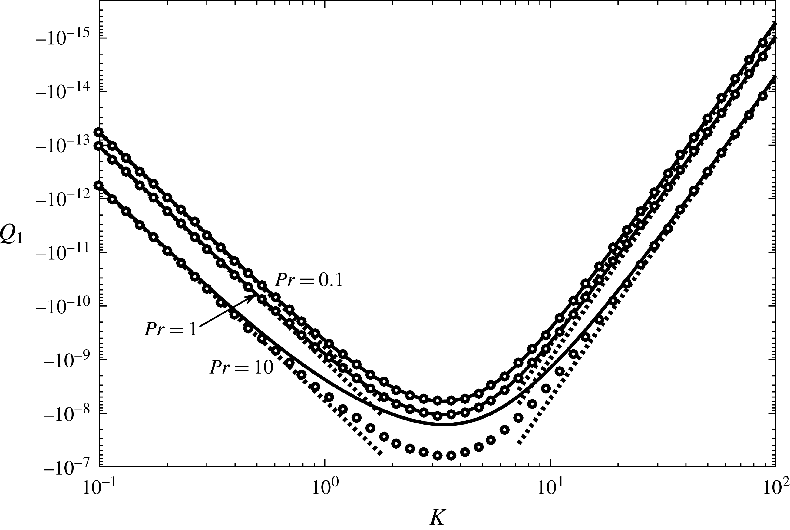
First-order volume flow rate
 $Q_{1}$
versus wavenumber
 $K$
for
 $Rc=1$
and various
 $Pr$
. The solid curves are the full solution of
 $Q_{1}$
calculated by the method described in appendix B. The dashed lines are the small and large
 $K$
asymptotic solutions (5.15) and (5.16), respectively. The open circles are the small
 $Rc$
asymptotic solution (5.5).

5.3 Wavenumber K
In figure 8,
 $Q_{1}$
is plotted as a function of
 $K$
for
 $Rc=1$
and various
 $Pr$
. It shows that
 $|Q_{1}|$
first increases with
 $K$
until
 $K\approx 3$
before decreasing. The behaviour of
 $Q_{1}$
as
 $K\rightarrow 0$
or
 $\infty$
makes physical sense. As
 $K\rightarrow 0$
, the thermal wavelength goes to infinity. In this limit, the thermal boundary condition at the bottom wall reduces to zero as shown by (2.6e
). Thus, there is no driving force and the axial volume flow rate vanishes. In the limit
 $K\rightarrow \infty$
, the thermal wavelength goes to zero, and the close proximity of temperature difference cancels itself. Thus, the driving force and therefore the axial volume flow rate again reduce to zero. The asymptotic analysis in the small and large limits of
 $K$
are similar to that of
 $Rc$
, so we only discuss the main points, leaving the mathematical details to appendix D.
In the limit
 $K\rightarrow 0$
, the expansion of
 $F(y)$
in (3.6a
) is regular, and the axial volume flow rate is found to be
 $$\begin{eqnarray}\displaystyle & \displaystyle Q_{1}=-{\displaystyle \frac{229(1+Pr)RcK^{4}}{435\,891\,456\,000}}+O(K^{5}). & \displaystyle\end{eqnarray}$$
This is plotted in figure 8 and agrees well with the full solution of
 $Q_{1}$
for
 $K\ll 1$
.
In the limit
 $K\rightarrow \infty$
, the expansion of
 $F(y)$
is singular. There is a boundary layer of thickness
 $O(K^{-1})$
near
 $y=0$
. The temperature variation and buoyancy driven flow are confined within this boundary layer. Outside the boundary layer, the temperature is uniform and the fluid is stationary. The axial volume flow rate is
 $$\begin{eqnarray}\displaystyle & \displaystyle Q_{1}=-{\displaystyle \frac{(1+Pr)Rc}{2048K^{6}}}+O(K^{-7}). & \displaystyle\end{eqnarray}$$
This is plotted in figure 8 and agrees well with the full solution of
 $Q_{1}$
for
 $K\gg 1$
. Since the boundary-layer thickness is
 $O(K^{-1})$
and the axial volume flow within the boundary layer is
 $Q_{1}\sim K^{-6}$
, it would be difficult for a numerical method to resolve this boundary layer, and to accurately calculate
 $Q$
.
5.4 Prandtl number
$Pr$

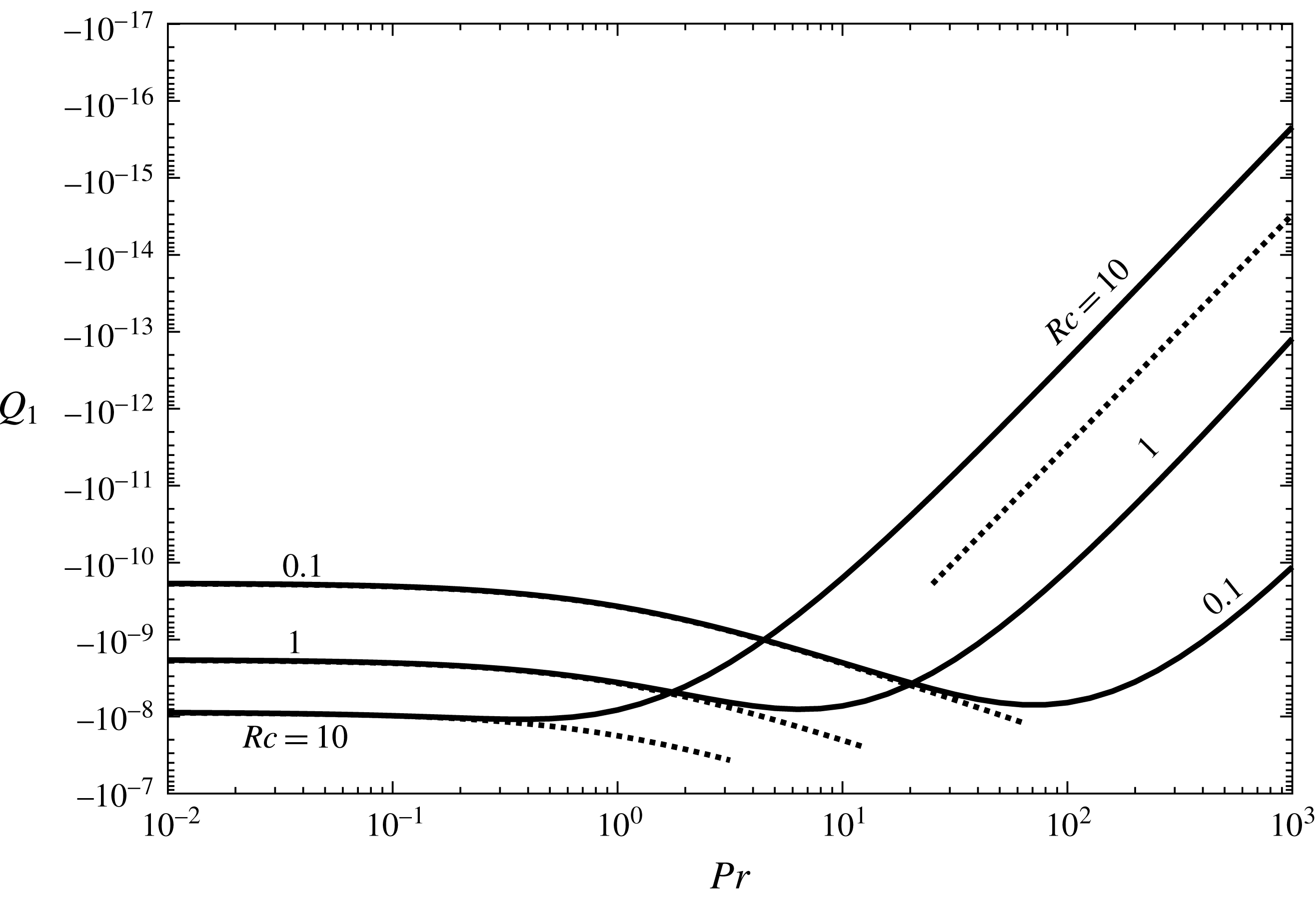
Figure 9 shows the dependence of
 $Q_{1}$
on
 $Pr$
. Since
 $Pr$
is a physical property of the fluid, it cannot be varied widely, and therefore the limit of
 $Pr\rightarrow 0$
or
 $\infty$
has little practical value. The limits also do not yield simpler equations. For these reasons, we do not seek asymptotic solutions and only briefly discuss the limiting behaviour.
The limit
 $Pr\rightarrow 0$
differs from the small
 $K$
or
 $Rc$
limit in that
 $Q$
approaches a non-zero constant, i.e. an axial flow exists for infinite thermal diffusivity (figure 9). The repetitive appearance of the relation
 $Q_{1}\propto (1+Pr)$
in previous sections suggests its wide applicability. Indeed,
 $Q_{1}=Q_{1}(Pr=0)~(1+Pr)$
fits the numerical solution very well, where the proportionality constant
 $Q_{1}(Pr=0)$
is the axial flow rate at
 $Pr=0$
and is calculated numerically. We note that for the curves with
 $Rc=0.1$
and
 $1$
in figure 9,
 $Q_{1}(Pr=0)$
can be calculated by the analytic solution in (5.5); for the curve with
 $Rc=10$
, equation (5.5) is not accurate. The large
 $Pr$
limit implies infinite viscosity or zero thermal diffusivity, and
 $Q_{1}$
vanishes. The scaling
 $Q_{1}\sim Pr^{-3}$
taken from the large
 $Rc$
asymptotic solution (5.14) captures the dependence quite well, although the proportionality constant is not straightforward to derive.
In figure 9, the curves with different
 $Rc$
cross as
 $Pr$
increases. This implies different dependence of
 $Q_{1}$
on
 $Rc$
as
 $Pr$
varies from infinitesimal to infinity. Figure 9 appears to suggest that
 $Q_{1}$
is proportional to
 $Rc$
as
 $Pr\rightarrow 0$
, and to
 $Rc^{-3}$
as
 $Pr\rightarrow \infty$
. A detailed analysis would be needed to validate this observation.
Figure 9 also shows that
 $|Q_{1}|$
reaches a maximum before decreasing as
 $Pr$
increases for fixed
 $K$
and
 $Rc$
. Similar behaviour of
 $Q_{1}$
is observed in figures 7 and 8 as
 $Rc$
and
 $K$
vary. We will take a close look at this in § 6.
First-order asymptotic volume flow rate
 $Q_{1}$
versus Prandtl number for
 $K=2\unicode[STIX]{x03C0}$
and various
 $Rc$
. The solid curves are the full solution of
 $Q_{1}$
calculated by the method described in appendix B. The dashed lines are the scaling
 $1+Pr$
as
 $Pr\rightarrow 0$
and
 $Pr^{-3}$
as
 $Pr\rightarrow \infty$
. All curves shown exhibit a maximum in
 $|Q_{1}|$
.

5.5 Discussion and comparison with previous work
Equations (5.15) and (5.16) describe how the axial flow rate
 $Q_{1}$
behaves in the limit the thermal wavenumber
 $K\rightarrow 0$
and
 $\infty$
, respectively. In each equation, the scaling with
 $K$
shows that the dependence is quite sensitive. It is interesting that
 $Q_{1}\propto (1+Pr)Rc$
in both small and large
 $K$
limits. For example, the large
 $K$
or ‘short wave limit’ corresponds to a thermal wave travelling beneath an infinitely deep channel. The axial flow rate is linearly proportional to how fast the thermal wave moves.
The asymptotic solutions (5.15) and (5.16) agree with the asymptotic solution (5.5) obtained in the limit
 $Rc\rightarrow 0$
when it is further expanded in the limits
 $K\rightarrow 0$
and
 $\infty$
. This is surprising because in deriving (5.5),
 $Rc$
is assumed to be small in the beginning, while in (5.15) and (5.16) no assumption is made about the magnitude of
 $Rc$
. In fact, a plot of (5.5) in figure 8 shows that it captures the variation of
 $Q$
for the entire range of
 $K$
when
 $Pr$
is small (0.1 and 1). For the larger
 $Pr=10$
value, it fails at intermediate
 $K$
values, where the large and small
 $K$
asymptotic solutions also do not hold.
While we could derive (5.15) and (5.16) from (5.5), we could not reverse the direction and derive the small and large
 $Rc$
asymptotic solutions from the small
 $K$
solution (5.15) by expanding it in the small and large
 $Rc$
limits, respectively. Mathematically this states the non-trivial relation among the different limits of parameters; while the limit
 $Rc\rightarrow 0$
can be swapped either with the limit
 $K\rightarrow 0$
or
 $K\rightarrow \infty$
, the limit
 $Rc\rightarrow \infty$
can neither be swapped with the limit
 $K\rightarrow 0$
nor with
 $K\rightarrow \infty$
.
The dependence of
 $Q$
on the thermal wave velocity has been well studied in the long wave limit (Stern Reference Stern1959; Davey Reference Davey1967). After translating their dimensionless groups to ours, the net volume flow rate given by Stern (Reference Stern1959) is
 $$\begin{eqnarray}\displaystyle Q_{1}=\left\{\begin{array}{@{}ll@{}}\displaystyle -5\times 10^{-7}RcK^{4} & KRc\,\text{small},\\[10.0pt] \displaystyle {\displaystyle \frac{1}{48\sqrt{2}}}Rc^{-5/2}K^{-1/2} & KRc\,\text{large}.\end{array}\right. & & \displaystyle\end{eqnarray}$$
The second expression says that
 $Q$
reverses its direction to be the same as the thermal wave, provided that
 $KRc$
is large enough (the threshold was estimated to be
 $10^{2}$
). Instead of assuming a volumetric temperature field, Davey (Reference Davey1967) used a more realistic approach and obtained
 $T(x,y)$
as a solution of the heat diffusion equation. Consequently,
 $Q_{1}$
was found to be
 $$\begin{eqnarray}\displaystyle Q_{1}=\left\{\begin{array}{@{}ll@{}}\displaystyle -{\displaystyle \frac{1+Pr}{12!}}RcK^{4} & KPrRc\,\text{small},\\[10.0pt] \displaystyle -{\displaystyle \frac{1}{4Pr^{2}(1+Pr)}}Rc^{-4}K^{-1} & KPrRc\,\text{large}.\end{array}\right. & & \displaystyle\end{eqnarray}$$
The dependence of
 $Q_{1}$
on
 $Rc$
and
 $K$
in the small
 $Rc$
limit differs from that of Stern (Reference Stern1959) only in the numerical coefficient. The dependence on
 $Pr$
is interesting as it shows that
 $Pr=0$
is a regular limit, which explains why the (volumetric temperature field) assumption made by Stern (Reference Stern1959) works. The large
 $Rc$
limit of
 $Q_{1}$
flows opposite to the thermal wave direction, and is proportional to
 $Rc^{-4}$
instead of
 $Rc^{-5/2}$
. These differences highlight how the initial simplification could qualitatively affect the result.
We do not make any initial simplification on
 $Rc$
,
 $K$
and
 $Pr$
. Our result has the same
 $(1+Pr)Rc$
dependence as the one obtained by Davey (Reference Davey1967). In the limit
 $K\rightarrow 0$
, equation (5.5) reduces to
 $$\begin{eqnarray}\displaystyle & \displaystyle Q_{1}=-{\displaystyle \frac{229(1+Pr)RcK^{4}}{435\,891\,456\,000}}. & \displaystyle\end{eqnarray}$$
Equation (5.19) results from taking two limits, first in
 $Rc\rightarrow 0$
and followed by
 $K\rightarrow 0$
. It is similar to the one by Davey (Reference Davey1967), with about
 $1/4$
the numerical coefficient value. This means that in the small
 $Rc$
and small
 $K$
limits, applying thermal waves at both walls generate four times greater axial flow rate, compared with applying the thermal wave at only one wall.
If we take
 $K\rightarrow \infty$
, equation (5.5) becomes
 $$\begin{eqnarray}\displaystyle & \displaystyle Q_{1}=-{\displaystyle \frac{(1+Pr)Rc}{2048K^{6}}}, & \displaystyle\end{eqnarray}$$
which differs from the large
 $KRc$
and large
 $KPrRc$
limits obtained by Stern (Reference Stern1959) and Davey (Reference Davey1967), respectively. This is expected as
 $K\rightarrow \infty$
is a ‘short wave’ limit, and is incompatible with the long wave assumption made by these authors. It may also be argued that the double limits of
 $Rc\rightarrow 0$
followed by
 $K\rightarrow \infty$
do not define the limit of their product
 $KRc$
. However, this is not a valid argument because (5.16), which is the same as (5.20), is derived in the limit
 $K\rightarrow \infty$
without any assumption on the magnitude of
 $Rc$
.
The large
 $Rc$
limit (5.14) is exactly half that of Davey (Reference Davey1967) reproduced above. This is because we apply the thermal wave only at the bottom wall, while in Davey (Reference Davey1967) the thermal wave is applied at both bottom and top walls. It is interesting that in the large
 $Rc$
limit, applying the thermal wave at both walls only double the axial flow rate, apparently due to all thermal effects being confined within the boundary layer.
6 Parametric study for maximum
$|Q_{1}|$

The first-order asymptotic volume flow rate
 $Q_{1}$
depends on
 $Rc$
,
 $K$
and
 $Pr$
. As shown in figures 7, 8 and 9,
 $|Q_{1}|$
versus
 $Rc$
,
 $K$
or
 $Pr$
always exhibits a maximum. In this section, we study the global maximum value of
 $|Q_{1}|$
and the corresponding values of
 $Rc$
,
 $K$
and
 $Pr$
. The results are needed for assessing the feasibility of using the travelling temperature wave as a driving mechanism in microchannel flow. The parameter space is searched by the following method. First, a set of
 $(Pr,K)$
pairs is generated with
 $0.01\leqslant Pr\leqslant 10$
and
 $0.25\leqslant K\leqslant 30$
. For each
 $(Pr,K)$
pair, we increase
 $Rc$
from 0.01 until
 $|Q_{1}|$
starts to decrease. The positions
 $(Rc_{m},Q_{1m})$
of the peak of
 $Q_{1}$
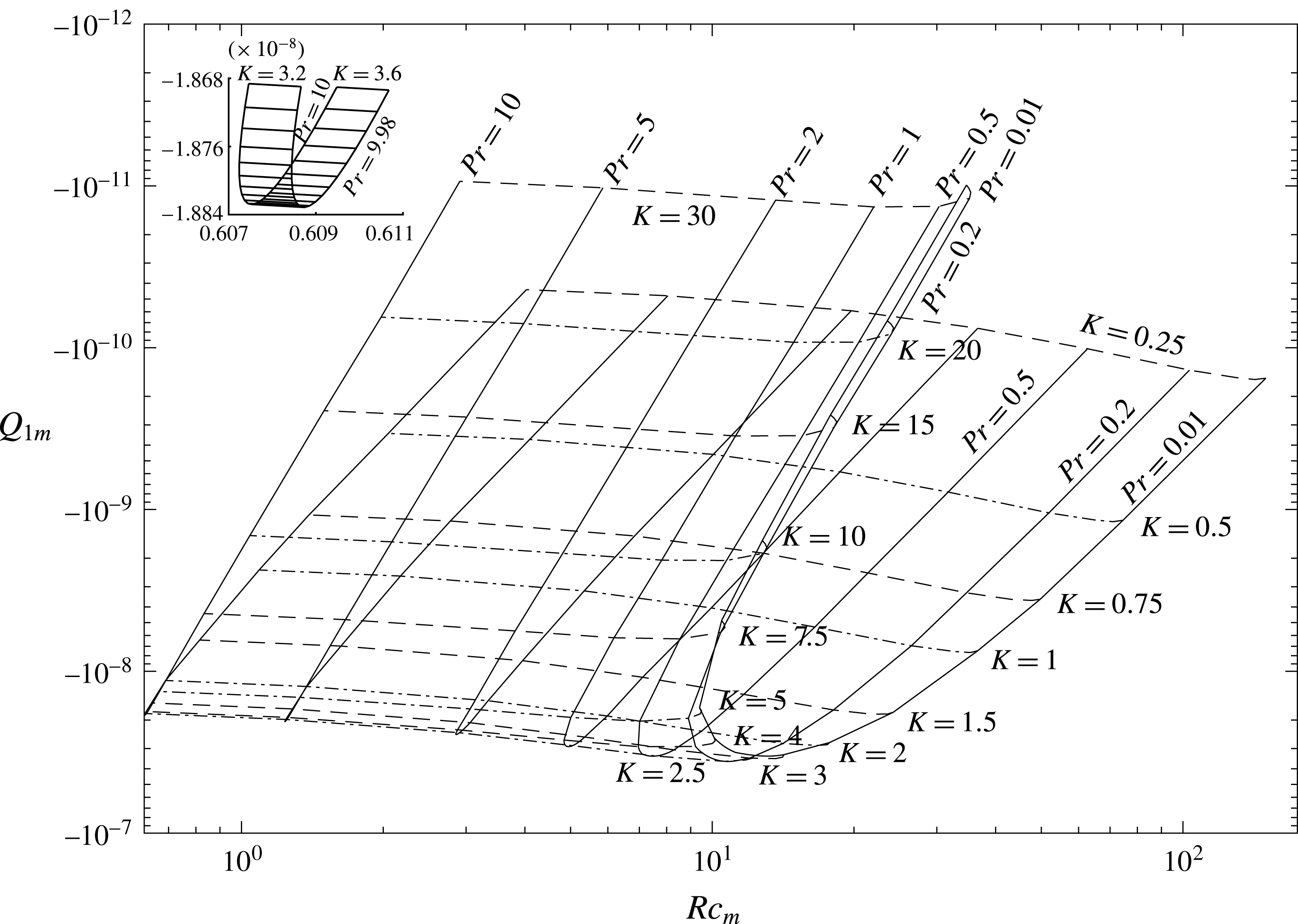
are located by a parabolic fit, and are plotted in figure 10. Thus,
 $Q_{1m}$
is a locally constrained maximum value of
 $Q_{1}$
, because
 $K$
and
 $Pr$
are fixed and
 $Rc$
varies. The results in figure 10 also reveal that there exists one and only one global maximum
 $Q_{1M}$
of
 $Q_{1}$
. At the global maximum, we find
 $Pr_{M}=0.168,K_{M}=2.89,Rc_{M}=10.9$
and
 $Q_{1M}=-3.61\times 10^{-8}$
.
The maximum value
 $Q_{1m}$
of
 $Q_{1}$
versus
 $Rc_{m}$
for various
 $K$
and
 $Pr$
. Each set of
 $(Rc_{m},K,Pr)$
locates a point in the parameter space where
 $Q_{1}$
reaches a locally constrained maximum with value
 $Q_{1m}$
. Constant
 $Pr$
curves are drawn in solid lines, while constant
 $K$
curves are drawn in dashed lines with alternating dash patterns. The inset is an expanded view of the ‘turning point’ of the
 $Pr=10$
curve.

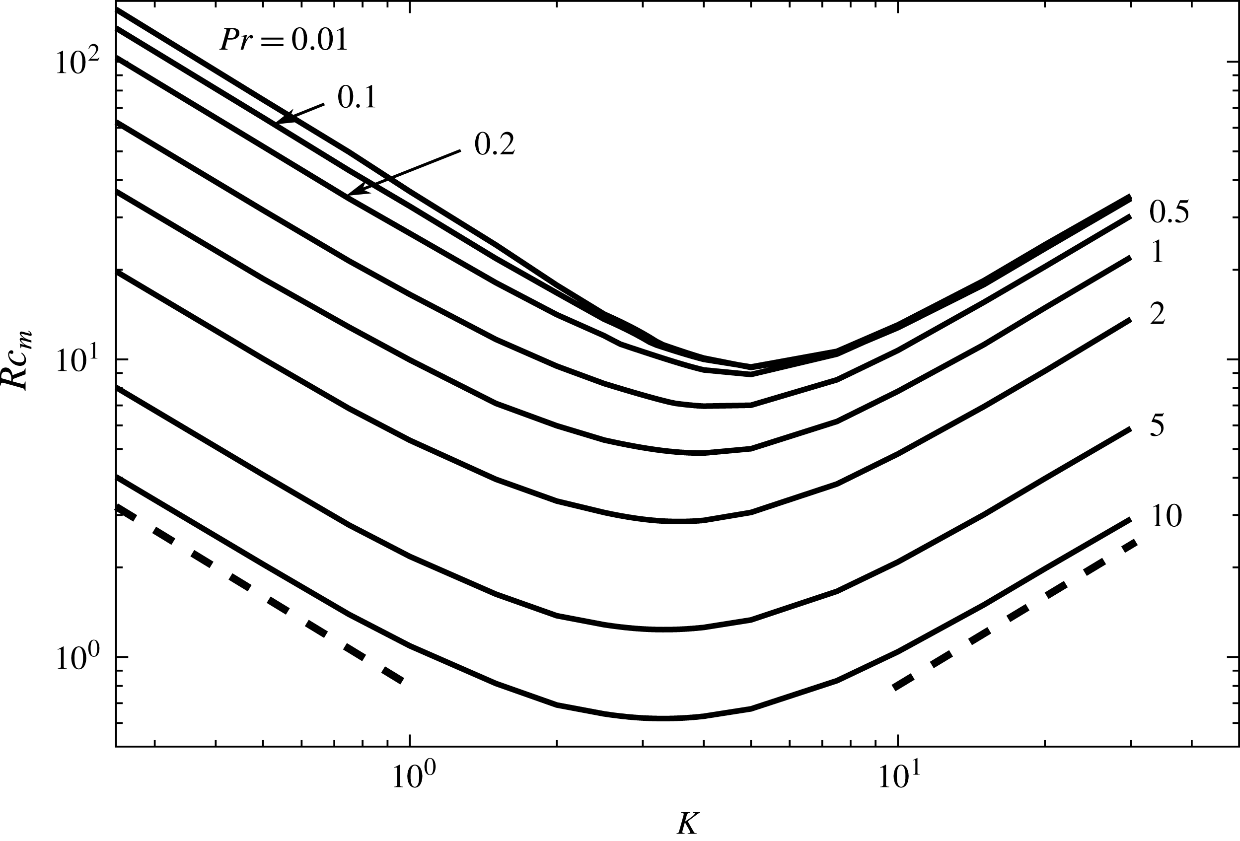
 $Rc_{m}$
versus
 $K$
for various
 $Pr$
from the data in figure 10. The left and right dashed lines represent
 $K^{-1}$
and
 $K$
scalings, respectively.

Figure 10 shows a surface in the parameter space folding onto itself. The crest of the fold represents maximum
 $|Q_{1m}|$
values, which occur in a narrow interval of
 $K$
, within
 $[2,4]$
by visual inspection, but are spread out over wide ranges of
 $Pr$
and
 $Rc_{m}$
. The fold appears to change from smooth to sharp as
 $Pr$
increases. This is only a visual artefact as shown by the upper left inset, which magnifies the crest of the leftmost
 $Pr=10$
curve. The surface not only folds in
 $K$
, but also in
 $Pr$
. This is visible from the curves with
 $Pr=0.01$
and
 $K\geqslant 15$
. Since this fold does not affect
 $Q_{1M}$
, it is not important and will not be studied.
Figure 10 shows that
 $Rc_{m}$
varies non-monotonically with
 $K$
and
 $Pr$
. To see these variations clearly,
 $Rc_{m}$
is plotted as a function of
 $K$
for various
 $Pr$
in figure 11. A physical argument can relate these parameters as follows. The system has two different time scales: the thermal wave time scale
 $\unicode[STIX]{x1D706}/c$
, and the thermal diffusivity time scale
 $h^{2}/\unicode[STIX]{x1D6FC}$
, where
 $\unicode[STIX]{x1D706}$
is the thermal wavelength. Balancing the two gives
 $c\sim \unicode[STIX]{x1D6FC}\unicode[STIX]{x1D706}/h^{2}$
, which becomes
 $Rc_{m}\sim Pr^{-1}K^{-1}$
when it is converted to the dimensionless groups. This scaling works if the thermal boundary-layer thickness is of order
 $h$
, i.e. the thermal effect penetrates the entire channel height. When
 $K$
is large, the vertical extension of the thermal effect is limited. The top wall appears as if it is located at infinity, so
 $h$
is no longer the proper scale of the thermal boundary layer. The only length scale in the system is the thermal wavelength
 $\unicode[STIX]{x1D706}$
. When
 $h$
is replaced by
 $\unicode[STIX]{x1D706}$
, we obtain another scaling
 $Rc_{m}\sim Pr^{-1}K$
. The argument here can be loosely compared with the driven damped harmonic oscillator in classical mechanics; the largest oscillation amplitude occurs when the system’s natural frequency matches the external forcing frequency. Figure 11 shows both scalings are correct in their respective
 $K$
limit. Following the above argument, the turning point of the curves in figure 11 corresponds to where the two scalings intercept, which happens at
 $K\sim 1$
.
7 Discussion
7.1 Flow pattern
We have shown that the nonlinearity is the cause of the horizontal axial flow, and derived an asymptotic solution that is valid for
 $Re=10^{3}$
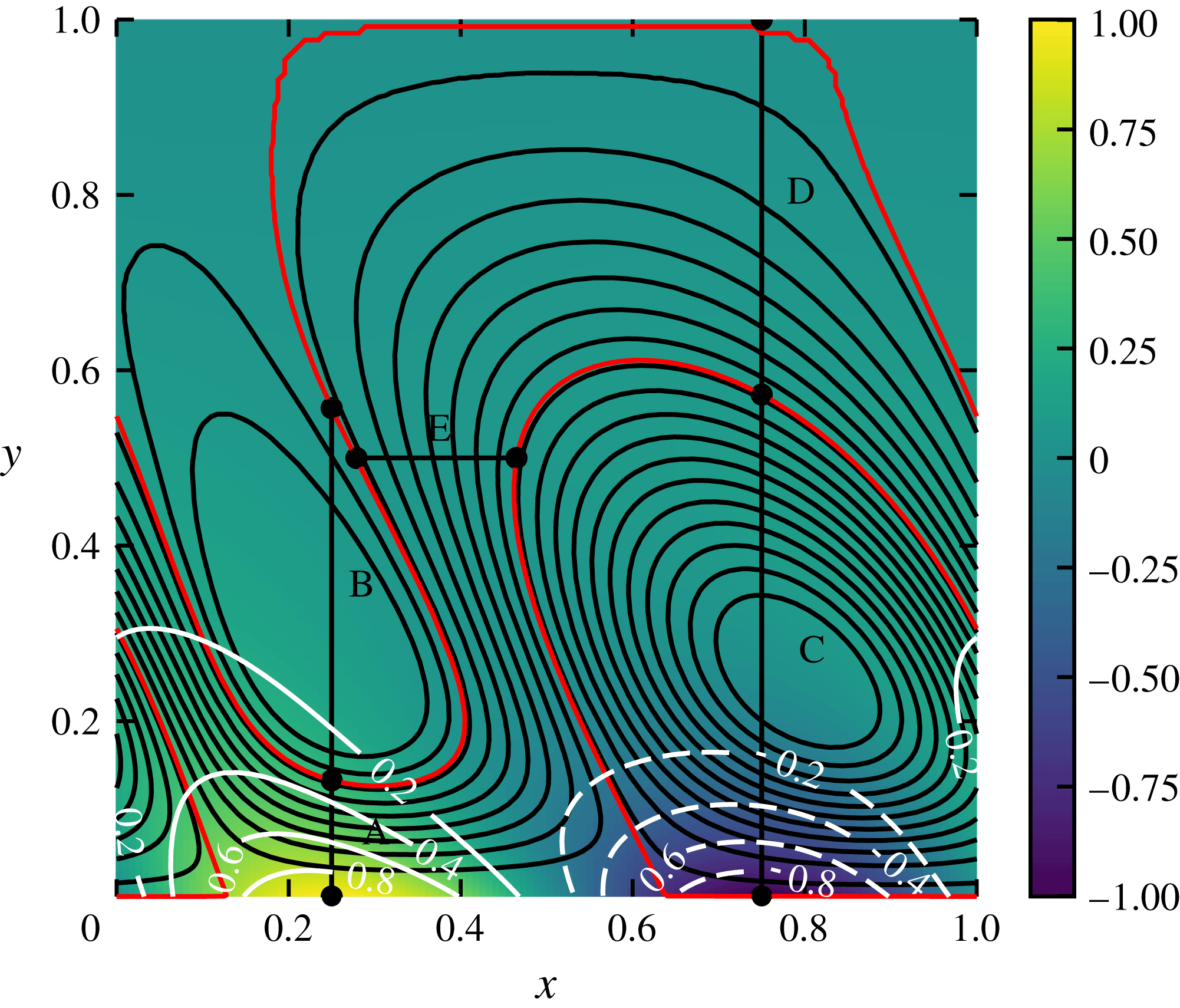
. However, the asymptotic solution does not capture the first-order flow field. It would be interesting to see the induced axial flows. Thus, we plot the computed flow field of a high Reynolds number case (
 $Re=10\,000,Rc=10,Pr=1,K=2\unicode[STIX]{x03C0}$
) in figure 12. This is the largest
 $Re$
case shown in figure 5.
Figure 12 shows that the flow field is characterized by isolated convective cells and, more importantly, a winding ‘stream’ in between the cells. Although this stream was discovered before by Young, Schubert & Torrance (Reference Young, Schubert and Torrance1972) in their numerical simulations (they called it a ‘channel’, we use ‘stream’ to avoid confusing it with the flow domain), the higher nonlinearity (greater stream width), shorter wavelength and unstretched aspect ratio give a closer look of the stream shape and its relative positioning to the isolated convective cells. We also check that the stream alone is responsible for the induced axial flow, i.e. integration of the flow across the stream gives the axial flow rate
 $Q$
(Young et al.
Reference Young, Schubert and Torrance1972). The sections in figure 12 span either across the stream or the convective cells. The flow rates of sections A, D and E are all close to the
 $Q$
value, while that of sections B and C are several orders of magnitude smaller. The disagreements for A, D and E are caused mainly by the interpolation error from locating the section ends. It is worth mentioning that the winding stream is narrower but still visible for
 $Re=2000$
(other parameters being the same), but is hardly so for
 $Re=1000$
or smaller.
Temperature contours and streamlines for
 $Re=10\,000$
,
 $Rc=10$
,
 $Pr=1$
and
 $K=2\unicode[STIX]{x03C0}$
. Both the white numbered contours and the colour plot show the temperature field. The solid black curves are the streamlines. The two separating streamlines are coloured in red. Five cross-sections (marked by capital letters) are used to calculate flow rates across them, which are
 $Q_{A}=-7.029\times 10^{-5},Q_{B}=-3.647\times 10^{-8},Q_{C}=-9.610\times 10^{-8},Q_{D}=-7.032\times 10^{-5}$
and
 $Q_{E}=-6.988\times 10^{-5}$
, while the axial volume flow rate is
 $Q=-7.032\times 10^{-5}$
.

7.2 Integral energy and force balances
The axial flow is driven by the travelling temperature wave, which generates a buoyancy force in the fluid in the vertical direction. However, this leads to a net horizontal axial flow. To investigate the driving force behind the net horizontal flow, we check the integral energy and force balances of the system. The thermal energy balance is checked by integrating the heat equation (2.6c ) over the domain volume. The left-hand side of (2.6c ) is first transformed into the conservative form:
 $$\begin{eqnarray}\displaystyle (Re\,\boldsymbol{u}-Rc\,\boldsymbol{i})\boldsymbol{\cdot }\unicode[STIX]{x1D735}T=\unicode[STIX]{x1D735}\boldsymbol{\cdot }[(Re\,\boldsymbol{u}-Rc\,\boldsymbol{i})T]. & & \displaystyle\end{eqnarray}$$
The volume integration of this term is converted into the surface integration
 $\oint [(Re\,\boldsymbol{u}-Rc\,\boldsymbol{i})T]\,\boldsymbol{\cdot }\,\text{d}\boldsymbol{S}$
over the domain boundary by the divergence theorem. The surface integral is zero over the top and bottom walls owing to the no-slip condition, and is zero over the left and right domain boundaries owing to periodicity. That means the volume integration of the right-hand side of (2.6c
) must also vanish, or
 $$\begin{eqnarray}\displaystyle \oint \unicode[STIX]{x1D735}T\boldsymbol{\cdot }\,\text{d}\boldsymbol{S}=0. & & \displaystyle\end{eqnarray}$$
Hence, heat energy entering the domain is equal to that leaving the domain and is not drained for driving the fluid motion. We numerically check the heat fluxes at the two walls for the case shown in figure 12 and found that they cancel each other, the difference between them being less than
 $10^{-4}\,\%$
.
The mechanical energy balance is checked by dotting the momentum equation with
 $\boldsymbol{u}$
and integrating over the domain. Using the divergence theorem and the wall and periodic boundary conditions, we find
 $$\begin{eqnarray}\displaystyle 2\int _{\bar{V}}\unicode[STIX]{x1D626}_{ij}\unicode[STIX]{x1D626}_{ij}\,\text{d}\bar{V}=\int _{\bar{V}}Tv\,\text{d}\bar{V}, & & \displaystyle\end{eqnarray}$$
where
 $v$
is the vertical velocity,
 $\unicode[STIX]{x1D626}_{ij}$
is the strain rate tensor and
 $\bar{V}$
is the domain volume. This is the same equation as in Davey (Reference Davey1967). It shows that the viscous dissipation of the flow field is balanced by the ‘thermal work’ instead of ‘thermal energy’. We numerically check the above equation for the flow field in figure 12; the total viscous dissipation and the thermal work differ by less than 0.1 %. Thus, the viscous dissipation of the induce axial flow in the channel must come from the thermal work. This energetics results from the Boussinesq approximation and was discussed in detail by Mihaljan (Reference Mihaljan1962). There it was demonstrated that ‘Boussinesq energy transformations and entropy production depend on the higher-order systems because of the peculiar simplification of the thermodynamic energy equation’. In other words, to capture the transformation between internal and kinetic energy requires the inclusion of the effect of compressibility, which is neglected by the Boussinesq approximation.
We check the integral force balance and find that the flow experiences zero total shear force on the walls. The momentum equation (2.6a ) is reproduced here and is integrated over the entire domain:
 $$\begin{eqnarray}\displaystyle (Re\,\boldsymbol{u}-Rc\,\boldsymbol{i})\boldsymbol{\cdot }\unicode[STIX]{x1D735}\boldsymbol{u}=-\unicode[STIX]{x1D735}p+\unicode[STIX]{x1D6FB}^{2}\boldsymbol{u}+T\boldsymbol{j}. & & \displaystyle\end{eqnarray}$$
The convection term is first converted into
 $\unicode[STIX]{x1D735}\boldsymbol{\cdot }(Re\,\boldsymbol{u}\boldsymbol{u}-Rc\,\boldsymbol{i}\boldsymbol{u})$
and then integrated:
 $$\begin{eqnarray}\displaystyle \int _{\bar{V}}\unicode[STIX]{x1D735}\boldsymbol{\cdot }(Re\,\boldsymbol{u}\boldsymbol{u}-Rc\,\boldsymbol{i}\boldsymbol{u})\,\text{d}\bar{V}=\oint (Re\,\boldsymbol{u}\boldsymbol{u}-Rc\,\boldsymbol{i}\boldsymbol{u})\boldsymbol{\cdot }\text{d}\boldsymbol{S}=\mathbf{0}. & & \displaystyle\end{eqnarray}$$
The surface integral vanishes owing to the no-slip and periodic boundary conditions. Integration of the pressure gradient term gives
 $$\begin{eqnarray}\displaystyle & \displaystyle \int _{\bar{V}}\unicode[STIX]{x1D735}p\,\text{d}\bar{V}=\oint p\,\text{d}\boldsymbol{S}=I_{1}\,\boldsymbol{j}, & \displaystyle\end{eqnarray}$$
where the horizontal forces cancel owing to periodicity, and only a net vertical force is left. Here,
 $I_{1}$
is a constant that depends on flow parameters. The Boussinesq forcing term integrates to
 $$\begin{eqnarray}\displaystyle & \displaystyle \int _{\bar{V}}T\boldsymbol{j}\,\text{d}\bar{V}=I_{2}\,\boldsymbol{j}, & \displaystyle\end{eqnarray}$$
which is also in the vertical direction. Here,
 $I_{2}$
is a constant that depends on flow parameters. The viscous term is integrated over the domain volume:
 $$\begin{eqnarray}\displaystyle & \displaystyle \int _{\bar{V}}\unicode[STIX]{x1D6FB}^{2}\boldsymbol{u}\,\text{d}\bar{V}=\oint _{S}\unicode[STIX]{x1D735}\boldsymbol{u}\boldsymbol{\cdot }\,\text{d}\boldsymbol{S}. & \displaystyle\end{eqnarray}$$
When all the integrated terms are substituted back to the momentum equation, we get
 $$\begin{eqnarray}\displaystyle & \displaystyle \oint _{S}\unicode[STIX]{x1D735}\boldsymbol{u}\boldsymbol{\cdot }\,\text{d}\boldsymbol{S}=(I_{1}-I_{2})\boldsymbol{j}. & \displaystyle\end{eqnarray}$$
Thus, there is no net horizontal shear force on the top and bottom walls. This is validated using the case in figure 12; the top and bottom walls experience opposite shear forces, with magnitudes that differ by less than
 $10^{-4}\,\%$
. Hence, there is no net shear force on the walls that resists or drives the axial flow. There is also no axial pressure gradient that drives the axial flow. The axial flow is induced solely by the Reynolds stress.
7.3 Integral energy and force balances of the asymptotic solutions
We also check the integral energy and force balances using the asymptotic solutions. The horizontally averaged temperature profile at the leading order,
 $\bar{T}_{0}(y)$
, is identically zero following (3.5b
). At the first order, the heat equation (3.10c
) is averaged in the axial direction over the thermal wavelength
 $2\unicode[STIX]{x03C0}/K$
to give
 $$\begin{eqnarray}\displaystyle & \displaystyle {\displaystyle \frac{\text{d}^{2}\overline{T}_{1}}{\text{d}y^{2}}}=Pr{\displaystyle \frac{\text{d}\overline{T_{0}v_{0}}}{\text{d}y}}. & \displaystyle\end{eqnarray}$$
This is integrated together with the boundary conditions
 $\bar{T}_{1}(0)=\bar{T}_{1}(1)=0$
to yield
 $$\begin{eqnarray}\displaystyle & \displaystyle \bar{T}_{1}(y)=Pr\int _{0}^{y}\left(\overline{T_{0}v_{0}}-\langle \overline{T_{0}v_{0}}\rangle \right)\text{d}\unicode[STIX]{x1D709}, & \displaystyle\end{eqnarray}$$
where the angle brackets denote vertical average over the channel height. Taking the
 $y$
-derivative and imposing the no-slip wall boundary condition, we obtain
 $$\begin{eqnarray}\displaystyle & \displaystyle {\displaystyle \frac{\text{d}\overline{T}_{1}}{\text{d}y}}=-Pr\langle \overline{T_{0}v_{0}}\rangle , & \displaystyle\end{eqnarray}$$
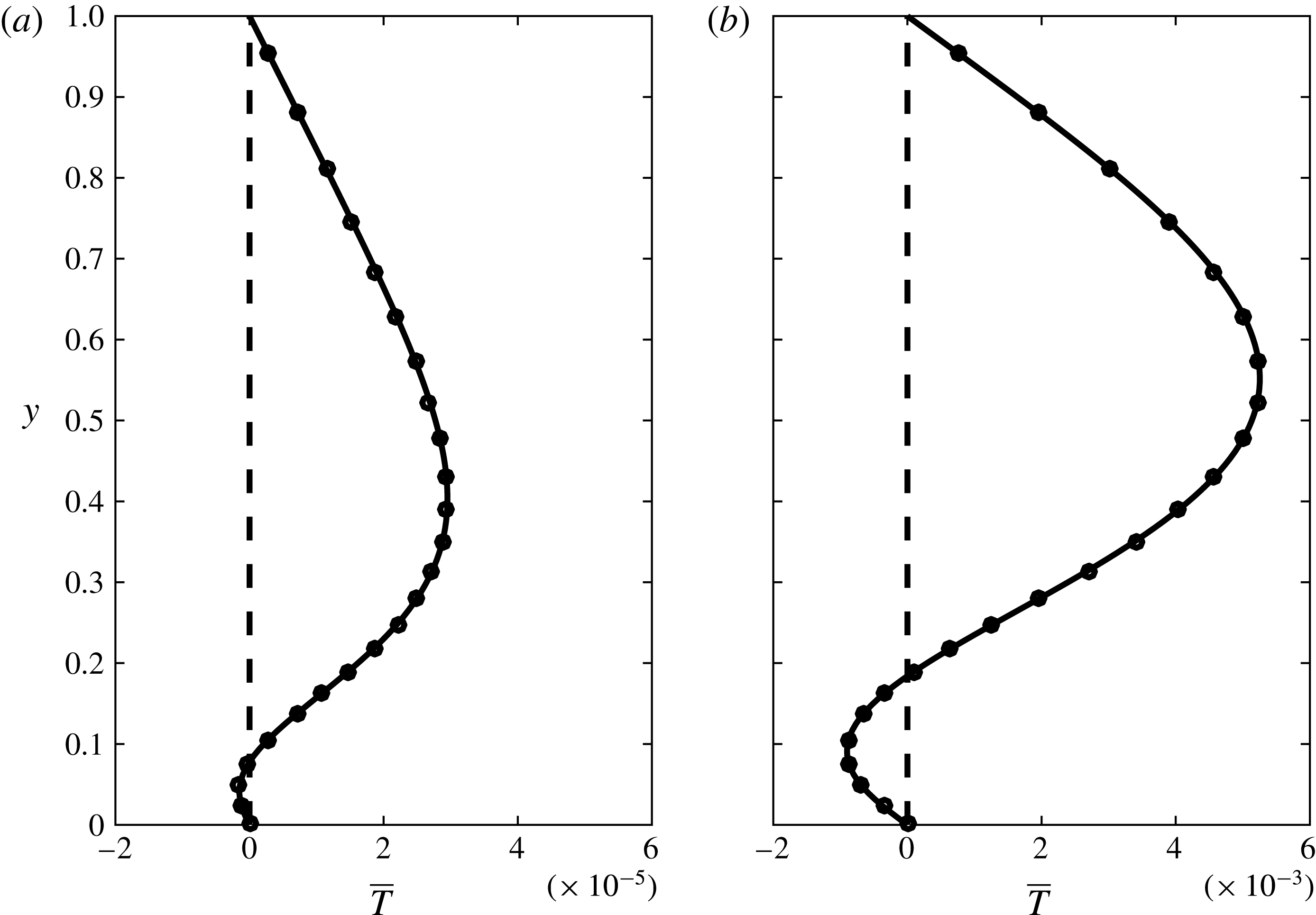
at both walls. Since the normals of the top and bottom walls are opposite, their heat fluxes cancel and no thermal energy is consumed by the fluid motion. Two typical temperature profiles corresponding to the cases in figures 2 and 3 are shown in figure 13 (note that
 $\bar{T}=Re\bar{T}_{1}(y)$
). It shows that the temperature gradients at the two walls are indeed the same.
The integral force balance is checked by studying the velocity gradients at the top and bottom walls. The leading-order horizontal velocity
 $u_{0}$
in (3.8) vanishes when averaged in the horizontal direction. The first-order solution in (3.13) gives
 $$\begin{eqnarray}\displaystyle & \displaystyle {\displaystyle \frac{\text{d}\overline{u}_{1}}{\text{d}y}}=\overline{u_{0}v_{0}}(y)-\langle \overline{u_{0}v_{0}}\rangle . & \displaystyle\end{eqnarray}$$
At both walls, the no-slip condition reduces the above equation to
 $$\begin{eqnarray}\displaystyle & \displaystyle {\displaystyle \frac{\text{d}\overline{u}_{1}}{\text{d}y}}=-\langle \overline{u_{0}v_{0}}\rangle . & \displaystyle\end{eqnarray}$$
The opposite normal directions of the top and bottom walls means their contributed shear stresses cancel each other. The averaged horizontal velocities plotted in figure 6 show that the gradients are indeed the same at the two walls. The zero net wall shear stress was mentioned in passing by Stern (Reference Stern1959) for his
 $\bar{u}_{1}$
solution. In Hinch & Schubert (Reference Hinch and Schubert1971), the averaged velocity profile was found to exert zero stress at both walls, which is likely caused by the long wave assumption made at the beginning of their work.
The horizontally averaged temperature profile
 $\bar{T}(y)$
. The cases in figures 2 and 3 are plotted in (a) and (b), respectively. Shown in each panel are the numerical solution (open circles), the leading-order asymptotic solution
 $\bar{T}_{0}$
(dashed line) and the first-order solution
 $Re\bar{T}_{1}$
(solid line).

7.4 Maximum induced axial flows
Our asymptotic expansions, which are accurate for
 $Re\leqslant 1000$
, give the induced axial volume flow rate
 $Q=ReQ_{1}(Rc,K,Pr)$
. The first-order flow rate
 $Q_{1}$
has a global maximum
 $Q_{1M}=-3.61\times 10^{-8}$
in the parameter space. We will use this maximum induced flow rate to investigate if the travelling temperature wave can be a practical driving mechanism.
The dimensional induced axial flow rate
 $Q^{\prime }=VhQ$
, following (2.5g
) where
 $V$
is the velocity scale given in (2.4). We consider a 2-D microchannel of height
 $h=1~\text{mm}$
, a travelling temperature wave of amplitude
 $A=10~^{\circ }\text{C}$
and two fluids: water and mercury, at room temperature. For water,
 $\unicode[STIX]{x1D708}=10^{-6}~\text{m}^{2}~\text{s}^{-1}$
and
 $\unicode[STIX]{x1D6FD}=2\times 1{0^{-4}~}^{\circ }\text{C}^{-1}$
. This gives
 $V=0.02~\text{m}~\text{s}^{-1}$
,
 $Re=20$
and
 $Q^{\prime }=VhRe|Q_{1M}|=1.4\times 10^{-5}~\text{mm}^{2}~\text{s}^{-1}$
, which is the volume flow rate per unit metre of channel width. This induced axial flow rate will yield a mean axial velocity of
 $1.4\times 10^{-5}~\text{mm}~\text{s}^{-1}$
, which is extremely small for practical applications.
For mercury,
 $\unicode[STIX]{x1D708}=10^{-7}~\text{m}^{2}~\text{s}^{-1}$
and
 $\unicode[STIX]{x1D6FD}=1.8\times 1{0^{-4}~}^{\circ }\text{C}^{-1}$
. Hence,
 $V=0.18~\text{m}~\text{s}^{-1}$
,
 $Re=1800$
and
 $Q^{\prime }=1.2\times 10^{-2}~\text{mm}^{2}~\text{s}^{-1}$
, which is still small.
Since
 $Q_{1M}=Q_{1}(Rc_{M},K_{M},Pr_{M})$
, we can control
 $Rc$
and
 $K$
to match the maximum-point values, but
 $Pr_{M}$
is a material property and cannot be varied easily. For the above two examples,
 $Pr=7.0$
for water and
 $Pr=0.025$
for mercury. As given in § 6,
 $Pr_{M}=0.168$
. Thus, the maximum achievable axial flow rates are even smaller than those calculated using
 $Q_{1M}$
.
7.5 Temperature wave imposed at the top wall instead
If the temperature wave is imposed at the top wall instead of the bottom wall (all other conditions being the same), the induced volume flow rate
 $Q$
is still the same. This is caused by the Boussinesq approximation. If we change
 $g\rightarrow -g$
in (2.1a
), then the microchannel is turned upside down, and the temperature is imposed at the top wall. However, if we further change
 $A\rightarrow -A$
in (2.1e
) and (2.5), then we recover the same system of equations (2.6). Thus, the induced axial flow rate
 $Q$
will be the same, i.e. it has the same magnitude and flows in the same direction (opposite to
 $c$
).
8 Conclusions
We study the axial flow in a 2-D microchannel induced by a travelling temperature wave imposed at the bottom wall. The Navier–Stokes equations with the Boussinesq approximation together with the convection–diffusion heat equation become steady in a reference frame moving with the travelling temperature wave. A velocity scale is determined by a dominant balance between the buoyancy and viscous forces in the vertical momentum equation. The governing equations and boundary conditions are made dimensionless by the velocity scale and the channel height, and four dimensionless groups emerge:
 $Re$
,
 $Rc$
,
 $K$
and
 $Pr$
. The problem is solved by a finite-volume method and by a perturbation method in the limit
 $Re\rightarrow 0$
. We find that the dimensionless axial volume flow rate
 $Q$
computed by the numerical method agrees with the perturbation solution for
 $Re\leqslant 1000$
. Thus, the analytic perturbation solution is used to study
 $Q$
and we obtain
 $Q=ReQ_{1}(Rc,K,Pr)$
. The first-order solution
 $Q_{1}$
is studied in detail as a function of
 $Rc$
,
 $K$
and
 $Pr$
. It is found for the first time that
 $Q_{1}$
has a global maximum
 $Q_{1M}$
(
 $=-3.61\times 10^{-8}$
) in the parameter space. Unfortunately, the extremely small magnitude of
 $Q_{1M}$
renders the travelling temperature wave not practical as a driving mechanism for microchannel flows.
Acknowledgements
C.Z. and K.N. acknowledge the financial support from the USDA-NIFA-AFRI grant and the Cain Chair Program. H.W. would like to acknowledge support from the Fritz & Frances M. Blumer Professorship during this work. Access to the High Performance Computing (HPC) facility at Louisiana State University is also gratefully acknowledged.
Appendix A. Analytic solution of
$F(y)$

Solution of (3.6a ) yields
 $$\begin{eqnarray}\displaystyle F(y)={\displaystyle \frac{K^{2}}{D}}(C_{1}\text{e}^{ry}+C_{2}\text{e}^{-ry}+C_{3}\text{e}^{qy}+C_{4}\text{e}^{-qy})+{\displaystyle \frac{K^{2}\csc (m)\sin [m(1-y)]}{m^{4}-2am^{2}+b}}, & & \displaystyle\end{eqnarray}$$
where
 $$\begin{eqnarray}\displaystyle a=K(\text{i}Rc-2K)/2,\quad b=-K^{3}(\text{i}Rc-K),\quad m=\sqrt{K(\text{i}RcPr-K)}, & & \displaystyle\end{eqnarray}$$
 $$\begin{eqnarray}\displaystyle s=\sqrt{a^{2}-b},\quad q=\sqrt{s-a},\quad r=\text{i}\sqrt{s+a}, & & \displaystyle\end{eqnarray}$$
 $$\begin{eqnarray}\displaystyle D & = & \displaystyle 2\left(m^{4}-2am^{2}+b\right)\left\{(\!a\left(\text{e}^{2q}-1\right)\left(\text{e}^{2r}-1\right)\right.\nonumber\\ \displaystyle & & \displaystyle \left.+\,qr\left[(\text{e}^{q}-\text{e}^{r})^{2}+(1-\text{e}^{q+r})^{2}\right]\right\},\end{eqnarray}$$
 $$\begin{eqnarray}\displaystyle C_{1} & = & \displaystyle (a-qr)\text{e}^{2q}+qr(2\text{e}^{q+r}-1)-a-s(\text{e}^{2q}-1)\nonumber\\ \displaystyle & & \displaystyle +\,m\left[(q+r)\text{e}^{2q}-2q\text{e}^{q+r}+q-r\right]\cot (m)\nonumber\\ \displaystyle & & \displaystyle +\,m\left[(q-r)\text{e}^{2q+r}+(q+r)\text{e}^{r}-2q\text{e}^{q}\right]\csc (m),\end{eqnarray}$$
 $$\begin{eqnarray}\displaystyle C_{2} & = & \displaystyle -\text{e}^{r}\left\{(a+qr)\text{e}^{2q+r}+(qr-a)\text{e}^{r}-2qr\text{e}^{q}-s\text{e}^{r}(\text{e}^{2q}-1)\right.\nonumber\\ \displaystyle & & \displaystyle \quad \left.+\,m\left[(q-r)\text{e}^{2q+r}+(q+r)\text{e}^{r}-2q\text{e}^{q}\right]\cot (m)\right.\nonumber\\ \displaystyle & & \displaystyle \quad \left.-\,m\left[2q\text{e}^{q+r}-(q+r)\text{e}^{2q}-q+r\right]\csc (m)\right\},\end{eqnarray}$$
 $$\begin{eqnarray}\displaystyle C_{3} & = & \displaystyle (a-qr)\text{e}^{2r}+qr(2\text{e}^{q+r}-1)-a+s(\text{e}^{2r}-1)\nonumber\\ \displaystyle & & \displaystyle +\,m\left[(q+r)\text{e}^{2r}-2r\text{e}^{q+r}-q+r\right]\cot (m)\nonumber\\ \displaystyle & & \displaystyle -\,m\left[(q-r)\text{e}^{q+2r}-(q+r)\text{e}^{q}+2r\text{e}^{r}\right]\csc (m),\end{eqnarray}$$
 $$\begin{eqnarray}\displaystyle C_{4} & = & \displaystyle -\text{e}^{q}\left\{(a+qr)\text{e}^{q+2r}+(qr-a)\text{e}^{q}-2qr\text{e}^{r}+s\text{e}^{q}(\text{e}^{2r}-1)\right.\nonumber\\ \displaystyle & & \displaystyle \quad \left.+\,m\left[(r-q)\text{e}^{q+2r}+(q+r)\text{e}^{q}-2r\text{e}^{r}\right]\cot (m)\right.\nonumber\\ \displaystyle & & \displaystyle \quad \left.-\,m\left[2r\text{e}^{q+r}-(q+r)\text{e}^{2r}+q-r\right]\csc (m)\right\}.\end{eqnarray}$$
Appendix B. Numerical method of calculating
$Q_{1}$

Due to the difficulty of separating the real and imaginary parts of the analytic solution of
 $F(y)$
in appendix A, we calculate
 $Q_{1}$
from it numerically. We first evaluate
 $F(y)$
in appendix A on 101 points uniformly distributed in
 $y$
. The derivative
 $\text{d}F/\text{d}y$
is then calculated using the second-order central difference. After separating the real and imaginary parts and multiplying them according to (3.15),
 $Q_{1}$
is found through (3.14) by applying the trapezoidal rule twice. Doubling the number of discretization points shows that
 $Q_{1}$
calculated this way has at least seven significant digits.
Appendix C. Asymptotic solution of
$Q_{1}$
in the limit
$Rc\rightarrow \infty$


C.1 Bottom boundary layer
The composite solution in (5.13) is
 $F_{c}(y)=f(y/\unicode[STIX]{x1D716})+F(y)-F_{m}$
, where
 $f=f_{R}+\text{i}f_{I}$
is complex, and both
 $F$
and
 $F_{m}$
are real. The composite solution is separated into real and imaginary parts and substituted into (3.15) to give the Reynolds stress:
 $$\begin{eqnarray}\displaystyle & \displaystyle \overline{u_{0}v_{0}}={\displaystyle \frac{1}{2K}}\left[f_{I}{\displaystyle \frac{\text{d}f_{R}}{\text{d}y}}-f_{R}{\displaystyle \frac{\text{d}f_{I}}{\text{d}y}}\right]+{\displaystyle \frac{1}{2K}}\left[f_{I}{\displaystyle \frac{\text{d}F}{\text{d}y}}-(F-F_{m}){\displaystyle \frac{\text{d}f_{I}}{\text{d}y}}\right]. & \displaystyle\end{eqnarray}$$
We find that the terms in the second square brackets are
 $O(\unicode[STIX]{x1D716})$
smaller than those in the first square brackets and can be neglected to leading order. Both terms in the first square brackets are of the same order, because
 $f_{I}\sim f_{R}$
and
 $\text{d}f_{I}/\text{d}y\sim \text{d}f_{R}/\text{d}y$
in the inner region where
 $y\sim \unicode[STIX]{x1D716}$
, as shown by the solution in (5.11). The solution also indicates that
 $f_{I}$
is exponentially small in the outer region where
 $y\gg \unicode[STIX]{x1D716}$
. Thus, the terms in the second square brackets only need to be considered in the inner region. If we compare the first term in both brackets, we find
 $(\text{d}F/\text{d}y)/(\text{d}f_{R}/\text{d}y)\sim \unicode[STIX]{x1D716}$
because the outer solution
 $F$
is slow varying in the inner region. If we compare the second term in both brackets, we find
 $(F-F_{m})/f_{R}\sim \unicode[STIX]{x1D716}$
because
 $\lim _{y\rightarrow 0}F\rightarrow F_{m}$
or
 $(F-F_{m})/F_{m}\sim y\sim \unicode[STIX]{x1D716}$
in the inner region. Since
 $f_{R}\sim F_{m}$
in the inner region, we get
 $(F-F_{m})/f_{R}\sim \unicode[STIX]{x1D716}$
. Thus, the terms in the second brackets can be neglected, and (C 1) becomes
 $$\begin{eqnarray}\displaystyle \displaystyle \overline{u_{0}v_{0}} & = & \displaystyle -{\displaystyle \frac{\unicode[STIX]{x1D716}^{7}}{2\sqrt{2K}(1-Pr)^{2}Pr^{3/2}}}\cdot \left\{(1-\sqrt{Pr})\text{e}^{-\left(1+\sqrt{Pr}\right)\unicode[STIX]{x1D707}}\sin \left[(1-\sqrt{Pr})\unicode[STIX]{x1D707}\right]\right.\nonumber\\ \displaystyle & & \displaystyle -\,(1+\sqrt{Pr})\text{e}^{-(1+\sqrt{Pr})\unicode[STIX]{x1D707}}\cos \left[(1-\sqrt{Pr})\unicode[STIX]{x1D707}\right]+\text{e}^{-2\sqrt{Pr}\unicode[STIX]{x1D707}}+\sqrt{Pr}\text{e}^{-2\unicode[STIX]{x1D707}}\nonumber\\ \displaystyle & & \displaystyle \left.+\,(1-\sqrt{Pr})\left[\text{e}^{-\unicode[STIX]{x1D707}}\left(\cos (\unicode[STIX]{x1D707})-\sin (\unicode[STIX]{x1D707})\right)-\text{e}^{-\sqrt{Pr}\unicode[STIX]{x1D707}}\left(\cos (\sqrt{Pr}\unicode[STIX]{x1D707})-\sin (\sqrt{Pr}\unicode[STIX]{x1D707})\right)\right]\right\},\nonumber\\ \displaystyle & & \displaystyle\end{eqnarray}$$
where
 $\unicode[STIX]{x1D707}=\sqrt{K/2}\cdot y/\unicode[STIX]{x1D716}$
. The Reynolds stress is integrated following (3.14) to give
 $$\begin{eqnarray}\displaystyle & \displaystyle Q_{1}=-{\displaystyle \frac{\unicode[STIX]{x1D716}^{8}}{8KPr^{2}(1+Pr)}}+O(\unicode[STIX]{x1D716}^{9}). & \displaystyle\end{eqnarray}$$
Thus, the induced volume flow rate comes only from the inner region at the leading order.
An interesting observation is that since the inner solution
 $f_{4}$
contains both real and imaginary parts, we do not need any higher-order term when forming
 $\overline{u_{0}v_{0}}$
in (C 1). This differs from the small
 $Rc$
limit, which involves a product between different perturbation orders. The reason is ultimately due to the asymptotic expansion of the ordinary differential equation in (3.6a
); it gives a real-coefficient equation (5.3a
) in the small
 $Rc$
limit, but a complex-coefficient equation (5.9) in the large
 $Rc$
limit.
C.2 Top boundary layer
The outer solution satisfies the no-penetration condition at the top wall, as shown in (5.7b
), but it does not satisfy the no-slip condition:
 $\text{d}F/\text{d}y(y=1)=0$
. Thus, another boundary layer is needed. To capture this top boundary layer, we define a set of inner variables:
 $\unicode[STIX]{x1D6FE}=(1-y)/\unicode[STIX]{x1D716}$
and
 $\unicode[STIX]{x1D714}(\unicode[STIX]{x1D6FE})=F(y)$
. The governing equation (5.6) becomes
 $$\begin{eqnarray}\displaystyle & \displaystyle {\displaystyle \frac{\text{d}^{4}\unicode[STIX]{x1D714}}{\text{d}\unicode[STIX]{x1D6FE}^{4}}}+K\left(\text{i}-2K\unicode[STIX]{x1D716}^{2}\right)\frac{\text{d}^{2}\unicode[STIX]{x1D714}}{\text{d}\unicode[STIX]{x1D6FE}^{2}}-\unicode[STIX]{x1D716}^{2}K^{3}\left(\text{i}-K\unicode[STIX]{x1D716}^{2}\right)\unicode[STIX]{x1D714}=0, & \displaystyle\end{eqnarray}$$
in which
 $G(y)$
has been dropped because it is exponentially small in the top boundary layer in the limit
 $\unicode[STIX]{x1D716}\rightarrow 0$
. The equation is subject to no-penetration and no-slip boundary conditions at the top wall at
 $\unicode[STIX]{x1D6FE}=0$
:
 $$\begin{eqnarray}\displaystyle \unicode[STIX]{x1D714}(0)=0\quad \text{and}\quad {\displaystyle \frac{\text{d}\unicode[STIX]{x1D714}}{\text{d}\unicode[STIX]{x1D6FE}}}(0)=0. & & \displaystyle\end{eqnarray}$$
The other two boundary conditions will come from matching to the outer solution. The inner variable is expanded in an asymptotic series in
 $\unicode[STIX]{x1D716}$
:
 $\unicode[STIX]{x1D714}=\unicode[STIX]{x1D714}_{0}(\unicode[STIX]{x1D6FE})+\unicode[STIX]{x1D716}\unicode[STIX]{x1D714}_{1}(\unicode[STIX]{x1D6FE})+\unicode[STIX]{x1D716}^{2}\unicode[STIX]{x1D714}_{2}(\unicode[STIX]{x1D6FE})+\cdots \,$
. Since the governing equation (C 4) and boundary conditions (C5) are homogeneous, and since the outer solution is
 $O(\unicode[STIX]{x1D716}^{4})$
,
 $\unicode[STIX]{x1D714}_{0}=\unicode[STIX]{x1D714}_{1}=\unicode[STIX]{x1D714}_{2}=\unicode[STIX]{x1D714}_{3}=0$
. Further,
 $\unicode[STIX]{x1D714}_{4}=0$
because
 $F_{4}=0$
at
 $y=1$
and
 $\text{d}F_{3}/\text{d}y=0$
. Thus, the first non-zero expansion is
 $\unicode[STIX]{x1D714}_{5}$
, which obeys
 $$\begin{eqnarray}\displaystyle & \displaystyle {\displaystyle \frac{\text{d}^{4}\unicode[STIX]{x1D714}_{5}}{\text{d}\unicode[STIX]{x1D6FE}^{4}}}+\text{i}K{\displaystyle \frac{\text{d}^{2}\unicode[STIX]{x1D714}_{5}}{\text{d}\unicode[STIX]{x1D6FE}^{2}}}=0. & \displaystyle\end{eqnarray}$$
The boundary conditions at
 $\unicode[STIX]{x1D6FE}=0$
give
 $$\begin{eqnarray}\displaystyle & \displaystyle \unicode[STIX]{x1D714}_{5}(0)={\displaystyle \frac{\text{d}\unicode[STIX]{x1D714}_{5}}{\text{d}\unicode[STIX]{x1D6FE}}}(0)=0. & \displaystyle\end{eqnarray}$$
The solution is
 $$\begin{eqnarray}\displaystyle \unicode[STIX]{x1D714}_{5}(\unicode[STIX]{x1D6FE}) & = & \displaystyle C_{1}\left[\text{e}^{-(1-\text{i})\sqrt{K/2}\unicode[STIX]{x1D6FE}}+(1-\text{i})\sqrt{K/2}\unicode[STIX]{x1D6FE}-1\right]\nonumber\\ \displaystyle & & \displaystyle +\,C_{2}\left[\text{e}^{(1-\text{i})\sqrt{K/2}\unicode[STIX]{x1D6FE}}-(1-\text{i})\sqrt{K/2}\unicode[STIX]{x1D6FE}-1\right].\end{eqnarray}$$
The asymptotic matching principle requires
 $$\begin{eqnarray}\displaystyle & \displaystyle \lim _{y\rightarrow 1}F(y)=\lim _{\unicode[STIX]{x1D6FE}\rightarrow \infty }\unicode[STIX]{x1D714}(\unicode[STIX]{x1D6FE})=F_{t}. & \displaystyle\end{eqnarray}$$
Keeping only leading-order terms, we have
 $$\begin{eqnarray}\displaystyle \lim _{y\rightarrow 1}F(y)=\lim _{y\rightarrow 1}\unicode[STIX]{x1D716}^{4}F_{4}(y)=-{\displaystyle \frac{\unicode[STIX]{x1D716}^{4}\text{e}^{K}\left[2K(1-y)\right]}{(\sqrt{Pr}+1)Pr(\text{e}^{2K}-1)}}, & & \displaystyle\end{eqnarray}$$
and
 $$\begin{eqnarray}\displaystyle & \displaystyle \lim _{\unicode[STIX]{x1D6FE}\rightarrow \infty }\unicode[STIX]{x1D714}(\unicode[STIX]{x1D6FE})=\lim _{\unicode[STIX]{x1D6FE}\rightarrow \infty }\unicode[STIX]{x1D716}^{5}\unicode[STIX]{x1D714}_{5}(\unicode[STIX]{x1D6FE})=\unicode[STIX]{x1D716}^{4}C_{1}\left[(1-\text{i})\sqrt{K/2}\right](1-y)+\unicode[STIX]{x1D716}^{5}C_{2}\text{e}^{(1-\text{i})\sqrt{K/2}\unicode[STIX]{x1D6FE}}. & \displaystyle\end{eqnarray}$$
This gives
 $$\begin{eqnarray}\displaystyle \left.\begin{array}{@{}l@{}}\displaystyle F_{t}=-{\displaystyle \frac{\unicode[STIX]{x1D716}^{4}\text{e}^{K}(2K)(1-y)}{(\sqrt{Pr}+1)Pr\cdot (\text{e}^{2K}-1)}},\\[10.0pt] \displaystyle C_{1}=-{\displaystyle \frac{(1+\text{i})\sqrt{2K}\text{e}^{K}}{(\sqrt{Pr}+1)Pr\cdot (\text{e}^{2K}-1)}},\\[10.0pt] \displaystyle C_{2}=0.\end{array}\right\} & & \displaystyle\end{eqnarray}$$
Since
 $\unicode[STIX]{x1D714}\sim \unicode[STIX]{x1D716}^{5}$
, it is one order smaller than
 $F$
and has no contribution to
 $Q_{1}$
at the leading order.
C.3 Numerical validation of the composite solution
The composite solution that includes both the bottom and top boundary layers has the form
 $$\begin{eqnarray}\displaystyle & \displaystyle F_{c}(y)=F+f(y/\unicode[STIX]{x1D716})+\unicode[STIX]{x1D714}((1-y)/\unicode[STIX]{x1D716})-F_{m}-F_{t}. & \displaystyle\end{eqnarray}$$
To test
 $F_{c}$
, we numerically compute a case with a relatively large
 $Rc$
value of 500. Other parameters are
 $Re=1,K=2\unicode[STIX]{x03C0}$
and
 $Pr=1$
. Note that for
 $K=2\unicode[STIX]{x03C0}$
and
 $x=1/4$
, equation (3.5a
) reduces to
 $v=\text{Re}[F_{c}(y)]$
, where
 $\text{Re}$
represents the real part. This solution of
 $v$
is plotted in figure 14 (dashed line) together with the numerical solution by OpenFOAM (open circles) and the analytic solution in appendix A (solid line). The composite solution matches the other two solutions quite well. The inset shows that the slope is indeed zero at the top wall, indicating the existence of the top boundary layer.
The composite solution
 $F_{c}$
has a non-zero gradient at the bottom wall (
 $y=0$
). Physically this means the
 $u$
velocity component, being proportional to
 $\text{d}F_{c}/\text{d}y$
, is non-zero at the bottom wall, and the flow slips. The no-slip condition can be imposed by including the
 $O(\unicode[STIX]{x1D716}^{5})$
term of the inner expansion at the bottom boundary layer, similar to the top boundary layer. Hence, its contribution to
 $Q_{1}$
is
 $O(\unicode[STIX]{x1D716}^{9})$
and can be neglected. Thus, we do not discuss that higher-order term here.
The vertical velocity
 $v(y)$
at
 $x=1/4$
as a function of
 $y$
for
 $Re=1$
,
 $Rc=500$
,
 $K=2\unicode[STIX]{x03C0}$
and
 $Pr=1$
. For
 $K=2\unicode[STIX]{x03C0}$
and
 $x=1/4$
, equation (3.5a
) gives
 $v(y)=\text{Re}[F_{c}(y)]$
. Shown together are the numerical solution (open circles), the leading-order asymptotic solution from appendix A (solid line) and the composite solution
 $F_{c}$
in (C 13) (dashed line). The inset is an expanded view of the top boundary layer.

Appendix D. Asymptotic solutions of
$Q_{1}$
as
$K\rightarrow 0$
and
$K\rightarrow \infty$


D.1 Asymptotic solution of
$Q_{1}$
in the limit
$K\rightarrow 0$


Instead of expanding the complex solution of
 $F(y)$
in appendix A, we find it more revealing to start from the governing equation (3.6a
), and expand
 $F$
in an asymptotic series in
 $K$
:
 $$\begin{eqnarray}\displaystyle & \displaystyle F(y)=F_{0}(y)+KF_{1}(y)+K^{2}F_{2}(y)+K^{3}F_{3}(y)+\cdots \,. & \displaystyle\end{eqnarray}$$
The source term in (3.6a
) contains
 $G(y)$
, the solution of which is presented in (3.7) and is expanded in an asymptotic series in
 $K$
:
 $$\begin{eqnarray}\displaystyle & \displaystyle G(y)=(1-y)+{\textstyle \frac{1}{6}}[y(1-y)(2-y)]\text{i}RcPrK+O(K^{2}). & \displaystyle\end{eqnarray}$$
These expansions are substituted into (3.6a,c ) to yield
 $$\begin{eqnarray}\displaystyle \left.\begin{array}{@{}c@{}}\displaystyle {\displaystyle \frac{\text{d}^{4}F_{0}}{\text{d}y^{4}}}=0,\\[7.0pt] \displaystyle {\displaystyle \frac{\text{d}^{4}F_{1}}{\text{d}y^{4}}}+\text{i}Rc{\displaystyle \frac{\text{d}^{2}F_{0}}{\text{d}y^{2}}}=0,\\[7.0pt] \displaystyle {\displaystyle \frac{\text{d}^{4}F_{2}}{\text{d}y^{4}}}+\text{i}Rc{\displaystyle \frac{\text{d}^{2}F_{1}}{\text{d}y^{2}}}-2{\displaystyle \frac{\text{d}^{2}F_{0}}{\text{d}y^{2}}}=1-y,\\[10.0pt] \displaystyle {\displaystyle \frac{\text{d}^{4}F_{3}}{\text{d}y^{4}}}+\text{i}Rc{\displaystyle \frac{\text{d}^{2}F_{2}}{\text{d}y^{2}}}-2{\displaystyle \frac{\text{d}^{2}F_{1}}{\text{d}y^{2}}}-\text{i}RcF_{0}(y)={\displaystyle \frac{1}{6}}\left[y(1-y)(2-y)\right]\text{i}RcPr,\\[10.0pt] \displaystyle F_{i}(0)=F_{i}(1)={\displaystyle \frac{\text{d}F_{i}}{\text{d}y}}(0)={\displaystyle \frac{\text{d}F_{i}}{\text{d}y}}(1)=0\quad \text{for}~i=0,1,2,3.\end{array}\right\} & & \displaystyle\end{eqnarray}$$
The above equations are solved in sequence to yield
 $$\begin{eqnarray}\displaystyle \left.\begin{array}{@{}l@{}}\displaystyle F_{0}(y)=0,\\[10.0pt] \displaystyle F_{1}(y)=0,\\[10.0pt] \displaystyle F_{2}(y)={\displaystyle \frac{1}{120}}y^{2}(1-y)^{2}(3-y),\\[10.0pt] \displaystyle F_{3}(y)={\displaystyle \frac{\text{i}Rc(1-y)^{2}y^{2}\left[19+37y-50y^{2}+10y^{3}+10Pr\left(11+3y-5y^{2}+y^{3}\right)\right]}{50\,400}}.\end{array}\right\}\quad & & \displaystyle\end{eqnarray}$$
The first two expansions of
 $F$
are zero because the source term in (3.6a
) is
 $O(K^{2})$
. Since
 $F_{2}$
is real, and
 $F_{3}$
is imaginary, equation (3.15) gives the Reynolds stress as
 $$\begin{eqnarray}\displaystyle & \displaystyle \overline{u_{0}v_{0}}={\displaystyle \frac{K^{4}}{2\text{i}}}\left({\displaystyle \frac{\text{d}F_{2}}{\text{d}y}}F_{3}-F_{2}{\displaystyle \frac{\text{d}F_{3}}{\text{d}y}}\right)+O(K^{5}). & \displaystyle\end{eqnarray}$$
As shown by the solutions of
 $F_{2}$
and
 $F_{3}$
in (D 4), the Reynolds stress has zero value, slope and curvature at the two walls. Between the two walls,
 $\overline{u_{0}v_{0}}$
reaches a maximum, similar to the profiles shown in figure 4. The first-order volume flow rate is then calculated from (3.14) as
 $$\begin{eqnarray}\displaystyle & \displaystyle Q_{1}=-{\displaystyle \frac{229(1+Pr)RcK^{4}}{435\,891\,456\,000}}. & \displaystyle\end{eqnarray}$$
We remark that a simple scaling argument by inspecting (3.6a
) could lead to erroneous result for
 $Q_{1}$
. Since the boundary condition of (3.6a
) is homogeneous, any non-trivial solution is driven by the source term
 $K^{2}G(y)$
. Thus, to leading order,
 $F\sim K^{2}$
, and then (3.14) and (3.15) give
 $Q_{1}\sim K^{3}$
, which is incorrect. This incorrect result is explained by (D 5), which shows the
 $O(K^{3})$
term vanishes on averaging over the wavelength, leaving the next
 $O(K^{4})$
term to be the correct leading order. Since the
 $O(K^{4})$
term involves the product of different expansion orders, it can only be found through the detailed analysis.
D.2 Asymptotic solution of
$Q_{1}$
in the limit
$K\rightarrow \infty$


In the limit
 $K\rightarrow \infty$
, the wavelength approaches zero, and the heating and cooling parts of the temperature wave cancel each other away from the wall. Thus, a boundary layer exists near the bottom wall, the thickness of which is scaled by the wavelength
 $K^{-1}$
. Thus, we define a small parameter as
 $\unicode[STIX]{x1D6FF}=1/K$
, and (3.6a
) becomes
 $$\begin{eqnarray}\displaystyle & \displaystyle \unicode[STIX]{x1D6FF}^{4}{\displaystyle \frac{\text{d}^{4}F}{\text{d}y^{4}}}-(2\unicode[STIX]{x1D6FF}^{2}-\text{i}\unicode[STIX]{x1D6FF}^{3}Rc){\displaystyle \frac{\text{d}^{2}F}{\text{d}y^{2}}}+(1-\text{i}\unicode[STIX]{x1D6FF}Rc)F=\unicode[STIX]{x1D6FF}^{2}G(y), & \displaystyle\end{eqnarray}$$
which is singular in the limit
 $\unicode[STIX]{x1D6FF}\rightarrow 0$
. In this limit,
 $G(y)\rightarrow \text{e}^{-(1/\unicode[STIX]{x1D6FF}-\text{i}RcPr/2)y}$
to leading order. In the inner region, we define a set of inner variables
 $\unicode[STIX]{x1D701}=y/\unicode[STIX]{x1D6FF},H(\unicode[STIX]{x1D701})=F(y)$
to resolve the boundary layer near
 $y=0$
, and (D 7) becomes
 $$\begin{eqnarray}\displaystyle & \displaystyle \displaystyle {\displaystyle \frac{\text{d}^{4}H}{\text{d}\unicode[STIX]{x1D701}^{4}}}-(2-\text{i}\unicode[STIX]{x1D6FF}Rc){\displaystyle \frac{\text{d}^{2}H}{\text{d}\unicode[STIX]{x1D701}^{2}}}+(1-\text{i}\unicode[STIX]{x1D6FF}Rc)H=\unicode[STIX]{x1D6FF}^{2}\text{e}^{-\unicode[STIX]{x1D701}}\left(1+\unicode[STIX]{x1D6FF}{\displaystyle \frac{1}{2}}\text{i}RcPr\unicode[STIX]{x1D701}\right). & \displaystyle\end{eqnarray}$$
In the limit
 $\unicode[STIX]{x1D6FF}\rightarrow 0$
,
 $H$
is expanded as
 $H=H_{0}(\unicode[STIX]{x1D701})+\unicode[STIX]{x1D6FF}H_{1}(\unicode[STIX]{x1D701})+\unicode[STIX]{x1D6FF}^{2}H_{2}(\unicode[STIX]{x1D701})+\unicode[STIX]{x1D6FF}^{3}H_{3}(\unicode[STIX]{x1D701})+\cdots \,$
. This is substituted into (D 8):
 $$\begin{eqnarray}\displaystyle \left.\begin{array}{@{}c@{}}\displaystyle {\displaystyle \frac{\text{d}^{4}H_{0}}{\text{d}\unicode[STIX]{x1D701}^{4}}}-2{\displaystyle \frac{\text{d}^{2}H_{0}}{\text{d}\unicode[STIX]{x1D701}^{2}}}+H_{0}=0,\\ \displaystyle {\displaystyle \frac{\text{d}^{4}H_{1}}{\text{d}\unicode[STIX]{x1D701}^{4}}}-2{\displaystyle \frac{\text{d}^{2}H_{1}}{\text{d}\unicode[STIX]{x1D701}^{2}}}+H_{1}=-\text{i}Rc\left({\displaystyle \frac{\text{d}^{2}H_{0}}{\text{d}\unicode[STIX]{x1D701}^{2}}}-H_{0}\right),\\ \displaystyle {\displaystyle \frac{\text{d}^{4}H_{2}}{\text{d}\unicode[STIX]{x1D701}^{4}}}-2{\displaystyle \frac{\text{d}^{2}H_{2}}{\text{d}\unicode[STIX]{x1D701}^{2}}}+H_{2}=-\text{i}Rc\left({\displaystyle \frac{\text{d}^{2}H_{1}}{\text{d}\unicode[STIX]{x1D701}^{2}}}-H_{1}\right)+\text{e}^{-\unicode[STIX]{x1D701}},\\ \displaystyle {\displaystyle \frac{\text{d}^{4}H_{3}}{\text{d}\unicode[STIX]{x1D701}^{4}}}-2{\displaystyle \frac{\text{d}^{2}H_{3}}{\text{d}\unicode[STIX]{x1D701}^{2}}}+H_{3}=-\text{i}Rc\left(\frac{\text{d}^{2}H_{2}}{\text{d}\unicode[STIX]{x1D701}^{2}}-H_{2}\right)+{\displaystyle \frac{1}{2}}\text{i}RcPr\unicode[STIX]{x1D701}\text{e}^{-\unicode[STIX]{x1D701}}.\end{array}\right\} & & \displaystyle\end{eqnarray}$$
The boundary conditions in (3.6c
) at
 $y=0$
give
 $$\begin{eqnarray}\displaystyle & \displaystyle H_{i}(0)={\displaystyle \frac{\text{d}H_{i}}{\text{d}\unicode[STIX]{x1D701}}}(0)=0\quad \text{for}~i=0,1,2,3\ldots . & \displaystyle\end{eqnarray}$$
Solution of (D 9) yields, after eliminating exponentially growing terms,
 $$\begin{eqnarray}\displaystyle \left.\begin{array}{@{}c@{}}\displaystyle H_{0}(\unicode[STIX]{x1D701})=0,\\ \displaystyle H_{1}(\unicode[STIX]{x1D701})=0,\\ \displaystyle H_{2}(\unicode[STIX]{x1D701})={\textstyle \frac{1}{8}}\text{e}^{-\unicode[STIX]{x1D701}}\unicode[STIX]{x1D701}^{2},\\ \displaystyle H_{3}(\unicode[STIX]{x1D701})={\textstyle \frac{1}{96}}\text{i}\text{e}^{-\unicode[STIX]{x1D701}}\unicode[STIX]{x1D701}^{2}Rc(2\unicode[STIX]{x1D701}+2(\unicode[STIX]{x1D701}+3)Pr+3).\end{array}\right\} & & \displaystyle\end{eqnarray}$$
In the outer region, the source term in (D 7) is exponentially small. Thus, the outer expansion yields a set of second-order, homogeneous ordinary differential equations (not shown). The boundary condition at
 $y=1$
is homogeneous. In addition, all inner solutions vanish in the limit
 $\unicode[STIX]{x1D701}\rightarrow \infty$
, so the matching condition for the outer solution in the limit
 $y\rightarrow 0$
is also homogeneous. For these reasons, the outer solution is null. Thus, the inner solution is the composite solution. Since
 $H_{2}$
is real and
 $H_{3}$
is imaginary, substitution of
 $F=H(\unicode[STIX]{x1D701})$
into (3.15) yields the Reynolds stress as
 $$\begin{eqnarray}\displaystyle \overline{u_{0}v_{0}}={\displaystyle \frac{\unicode[STIX]{x1D6FF}^{5}}{2\text{i}}}\left({\displaystyle \frac{\text{d}H_{2}}{\text{d}\unicode[STIX]{x1D701}}}H_{3}-H_{2}{\displaystyle \frac{\text{d}H_{3}}{\text{d}\unicode[STIX]{x1D701}}}\right)+O(\unicode[STIX]{x1D6FF}^{6})=-{\displaystyle \frac{(1+Pr)Rc}{768}}\unicode[STIX]{x1D6FF}\text{e}^{-2y/\unicode[STIX]{x1D6FF}}y^{4}+O(\unicode[STIX]{x1D6FF}^{6}). & & \displaystyle\end{eqnarray}$$
Thus, the Reynolds stress is extremely flat as it approaches both walls. Away from the walls, it shows a maximum, which occurs at
 $y=2\unicode[STIX]{x1D6FF}$
. The first-order volume flow rate is found from (3.14) as
 $$\begin{eqnarray}\displaystyle Q_{1}=-{\displaystyle \frac{(1+Pr)Rc}{2048K^{6}}}+O(K^{-7}). & & \displaystyle\end{eqnarray}$$
In the limit
 $K\rightarrow \infty$
, the temperature wave drives fluid motion only in a boundary layer of thickness
 $O(K^{-1})$
near the bottom wall. Outside the boundary layer, the fluid is stationary. Within the boundary layer, there is still an induced axial flow, although the magnitude is small.