1 Introduction
The aim of the present investigation, which developed from our initial study into skin-friction critical points in wall-bounded flows (Cardesa et al. Reference Cardesa, Monty, Soria and Chong2014), is to bring further insights into the near-wall structure of turbulent wall-bounded flow and its connection and potential dynamical interaction with the larger structures found in the outer layer of these flows. Specifically, this study is focused on studying in detail the rare backflow or reverse flow events which appear very close to the wall in turbulent wall-bounded flows, in order to understand their possible connection with large-scale structures which develop much further from the wall.
The occurrence of near-wall backflow in turbulent wall-bounded flows, and with it the presence of negative values of the local wall shear stress, have been the subject of debate for the past decades. Eckelmann (Reference Eckelmann1974) postulated that near-wall backflow in wall-bounded turbulent flows was not possible, and experimentalists did not observe this somewhat counter-intuitive flow phenomenon until the recent detailed experimental studies by Willert et al. (Reference Willert, Cuvier, Foucaut, Klinner, Stanislas, Laval, Srinath, Soria, Amili and Atkinson2018a
) in zero pressure gradient turbulent boundary layers (ZPG TBL) and Willert et al. (Reference Willert, Soria, Cuvier, Foucaut and Laval2018b
,Reference Willert, Soria, Cuvier, Foucaut and Laval
c
) in turbulent boundary layers with varying pressure gradients. However, even early direct numerical simulations (DNS) suggested the opposite, such as the DNS of ZPG TBL by Spalart & Coleman (Reference Spalart and Coleman1997), who found events of negative shear stress, and the turbulent channel flow DNS of Hu, Morfey & Sandham (Reference Hu, Morfey and Sandham2006). Similar observations were subsequently made in more recent DNS of turbulent channel flow and ZPG TBL by Lenaers et al. (Reference Lenaers, Li, Brethouwer, Schlatter and Örlü2012). Negative wall shear stress events were also observed in the turbulent pipe flow DNS by El Khoury et al. (Reference El Khoury, Schlatter, Brethouwer and Johansson2014) and Jalalabadi & Sung (Reference Jalalabadi and Sung2018). Cardesa et al. (Reference Cardesa, Monty, Soria and Chong2014), in addition to confirming the existence of areas of vanishing wall shear stress in DNS of turbulent channel flow at
 $Re_{\unicode[STIX]{x1D70F}}=934$
and
 $Re_{\unicode[STIX]{x1D70F}}=1834$
, associated skin-friction critical points with large-scale structures that extend up to 800 wall units downstream. Diaz-Daniel, Laizet & Vassilicos (Reference Diaz-Daniel, Laizet and Vassilicos2017) proposed a model relating the skin friction at the wall and fluctuating velocities inside the boundary layer.
In the present study, DNS of turbulent channel flows ranging from
 $Re_{\unicode[STIX]{x1D70F}}=547$
to 2003 were used to investigate the probability of finding backflow regions in wall-bounded turbulent flows as a function of wall distance, as well as to investigate the lifetime, convection velocity and three-dimensional structure of these near-wall backflow regions. Conditional dynamical analysis is employed to investigate the link between the backflow regions in the viscous sublayer and the
 $Re_{\unicode[STIX]{x1D70F}}$
-dependent dynamics of much larger structures further away from the wall, and is reported in this paper.
2 Numerical simulations and data processing
The raw data for this study is available from the public databases of the Technical University of Madrid, at the following url: torroja.dmt.upm.es/turbdata/raw_database/Channels. In particular, we use the flow fields from cases
 $Re550$
(del Álamo & Jiménez Reference del Álamo and Jiménez2003),
 $Re950$
(del Álamo et al.
Reference del Álamo, Jiménez, Zandonade and Moser2004) and
 $Re2000$
(Hoyas & Jiménez Reference Hoyas and Jiménez2006) described in table 1. They were computed by DNS of an incompressible channel flow with periodic boundary conditions in the streamwise (
 $x$
) and spanwise (
 $z$
) directions, along which space was Fourier-decomposed. The wall-normal direction
 $y$
was discretized with a Chebyshev collocation method and seven-point compact finite differences for
 $Re_{\unicode[STIX]{x1D70F}}\leqslant 1000$
and
 $Re_{\unicode[STIX]{x1D70F}}>1000$
, respectively. We label velocities along
 $(x,y,z)$
as
 $(u,v,w)$
, while quantities in wall units (normalized by kinematic viscosity
 $\unicode[STIX]{x1D708}$
and friction velocity
 $u_{\unicode[STIX]{x1D70F}}$
) feature a ‘
 $+$
’ superscript. The snapshots in cases
 $Re550$
,
 $Re950$
and
 $Re2000$
are separated by long time intervals, so we ran an additional case to time-track coherent structures with very small time scales. This is case
 $Re950TR$
(Cardesa et al.
Reference Cardesa, Monty, Soria and Chong2014) in table 1, with a fixed DNS time step of
 $0.02^{+}$
and consecutive snapshots stored every
 $0.3^{+}$
. The sequence spans
 $889.5^{+}$
, almost one eddy turnover
 $h/u_{\unicode[STIX]{x1D70F}}$
– where
 $h$
is the channel half-height. All DNS are based on the wall-normal vorticity
 $\unicode[STIX]{x1D714}_{y}$
and
 $\unicode[STIX]{x1D6FB}^{2}v$
formulation of Kim, Moin & Moser (Reference Kim, Moin and Moser1987), using a third-order semi-implicit Runge–Kutta scheme for time integration. The simulations ran at constant mass flux rate.
We cluster the regions of the flow that fulfil
 $u<0$
into labelled objects. Each object is defined as a collection of connected grid points (or cells) which share the
 $u<0$
condition. The clustering algorithm probed all 26 neighbouring cells for connections and accounted for the domain periodicity. We store the objects, or flow structures thus obtained, for their statistical characterization. The smallest building block of an object is a single grid cell, with length
 $\unicode[STIX]{x0394}x^{+}$
and span
 $\unicode[STIX]{x0394}z^{+}$
, both scaled by
 $2/3$
. This is due to the fact that we compute
 $u$
on the dealiased grid obtained by zero-padding in Fourier space following the
 $3/2$
rule. In the
 $Re950TR$
case, we use the stored objects as input to the time-tracking algorithm developed and used in Lozano-Durán & Jiménez (Reference Lozano-Durán and Jiménez2014). This allows us to follow the objects in time and study their dynamics.
DNS details of the channel flows used in this study.
 $h$
is the channel half-height,
 $L_{x}$
and
 $L_{z}$
are the channel dimensions in the streamwise and spanwise directions, respectively, while
 $\unicode[STIX]{x0394}x^{+}$
and
 $\unicode[STIX]{x0394}z^{+}$
are the resolutions in those directions before dealiasing.
 $N_{y}$
is the number of grid points in the wall-normal direction. The full grid in
 $y$
, along with other statistics for these channels, can be found at the following url: torroja.dmt.upm.es/channels/data.
 $N_{f}$
is the number of independent flow fields used, except for
 $Re950TR$
, where the fields are sampled at a high-frequency rate for time-tracking.
 $N_{s}$
is the number of extracted flow structures based on
 $u<0$
. For
 $Re950TR$
, one in every five fields is used to obtain
 $N_{s}$
, and these structures were added to the pool of structures of the
 $Re950$
case. Hence the structures of
 $Re950$
and
 $Re950TR$
were merged to obtain the grey line data sets on figure 1.
 $n_{A}$
is the mean number of backflow structures per million wall square units, given with 99 % confidence intervals.

3 Probability of backflow
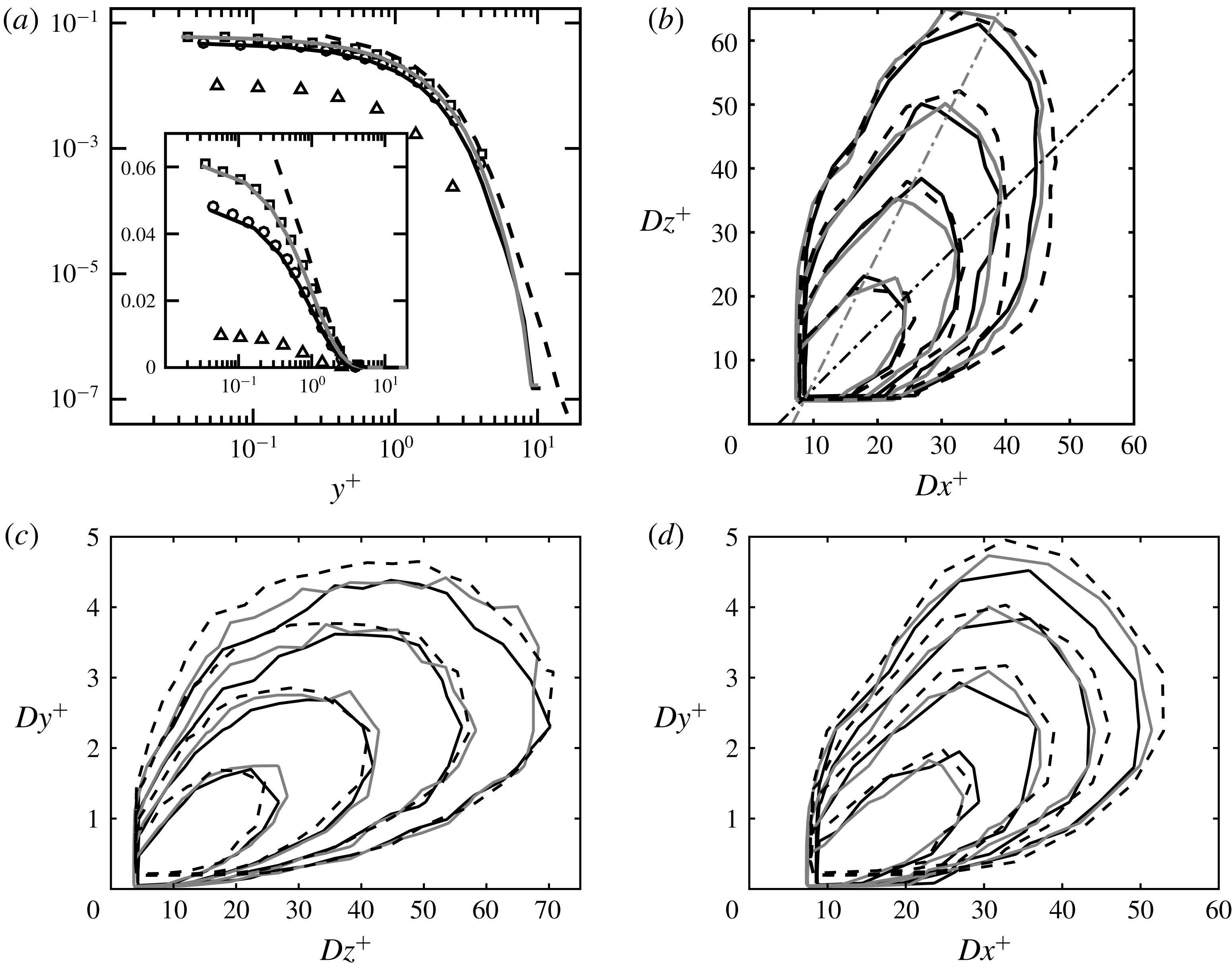
Line series as detailed in table 1, with cases
 $Re950$
and
 $Re950TR$
merged. (a) Percentage of backflow as a function of wall distance. Empty symbols are data extracted from figure 4(a) in Lenaers et al. (Reference Lenaers, Li, Brethouwer, Schlatter and Örlü2012) with g3data (Bauer & Reynolds Reference Bauer and Reynolds2008):
 ${\vartriangle}$
 $Re_{\unicode[STIX]{x1D70F}}=179$
,
 $\circ$
 $Re_{\unicode[STIX]{x1D70F}}=586$
,
 $\Box$
 $Re_{\unicode[STIX]{x1D70F}}=1000$
, which are cases labelled as 180 m, 590 m and 1000 m, respectively, in Lenaers et al. (Reference Lenaers, Li, Brethouwer, Schlatter and Örlü2012). The inset shows the same data on a semi-log scale. (b) Joint probability density function (JPDF) of length and width of backflow regions at three Reynolds numbers. Contour levels enclose 40 %, 70 %, 85 % and 92.5 % of the total probability. Dash-dotted straight lines follow
 $Dz^{+}=c_{1}Dx^{+}+c_{2}$
, where
 $c_{1}=1$
(black) and
 $c_{1}=2$
(grey).
 $c_{2}$
is set so that both lines intersect at
 $Dx^{+}=2\unicode[STIX]{x0394}x^{+}/3$
and
 $Dz^{+}=2\unicode[STIX]{x0394}z^{+}/3$
of
 $Re550$
on table 1. (c) JPDF of height and width of backflow regions at three Reynolds numbers. Same contour levels as in (b). (d) JPDF of height and length of backflow regions at three Reynolds numbers. Same contour levels as in (b).

We plot the percentage of backflow as a function of height on figure 1(a), along with the data from Lenaers et al. (Reference Lenaers, Li, Brethouwer, Schlatter and Örlü2012). The two highest Reynolds numbers in that study almost match our
 $Re550$
and
 $Re950$
cases, leading to the good agreement between the corresponding data sets on figure 1(a). Note that the first grid point away from the wall is located at
 $y^{+}=\{0.32,~0.031,~0.041\}$
in the
 $Re2000$
,
 $Re950$
and
 $Re550$
cases, respectively. The last two cases feature a Chebyshev-based discretization in the wall-normal direction and hence a higher resolution in
 $y$
than the
 $Re2000$
case. This explains why the first entry in the
 $Re2000$
case is further from the wall compared to the other data sets. Up to
 $y^{+}=4$
, all three cases support the trend of a higher proportion of flow reversal as the Reynolds number increases. It is very probable that the trend persists above this height, but we cannot remain conclusive based on our data since the events become so infrequent that sample size effects have a significant impact. Table 1 shows that
 $Re2000$
is by far our most abundant data set in terms of flow structures
 $N_{s}$
, with almost an order of magnitude more data than the other cases. This explains why events with probabilities below
 $10^{-7}$
are observable for the
 $Re2000$
case and not the others.
Mean dimension along
 $x,y$
and
 $z$
of the bounding box of the negative backflow regions (first three columns). Percentage of objects composed of only one grid cell along coordinates (a)
 $x$
, (b)
 $y$
, (c)
 $z$
, (d)
 $x$
and
 $z$
, (e)
 $x$
,
 $z$
and
 $y$
. (f) Percentage of objects on the upper side of the channel. (g) Percentage of wall-attached objects.

4 Structure of backflow objects
After isolating all individual backflow objects, we analyse their size distributions along the three coordinates. We plot the two-dimensional joint probability distributions (JPDFs) of combinations of length (
 $Dx^{+}$
), height (
 $Dy^{+}$
) or width (
 $Dz^{+}$
) of the rectangular bounding box of the objects on figure 1(b–d). All objects found are attached to the wall in cases
 $Re550$
,
 $Re950$
and
 $Re950TR$
, while 99.96 % of objects in
 $Re2000$
are attached – see table 2.
 $Dy^{+}$
can therefore be considered as the distance of the upper end of the flow structures to the wall. The contour levels on figure 1(b–d) are equal for all three Reynolds numbers, and share many similarities. However, it is difficult to draw definite conclusions regarding their collapse in viscous units, chiefly due to the sample sizes affecting mostly the largest objects.
It is apparent from figures 1(c) and 1(d) that the length and width of backflow regions are significantly greater than their height. We are therefore studying flow objects that resemble flattened separation bubbles. To help assess the relation between their width and length, figure 1(b) shows two straight dash-dotted lines along
 $Dz^{+}\propto Dx^{+}$
and
 $Dz^{+}\propto 2Dx^{+}$
. Because the spacing between grid points in
 $x$
is exactly double that in
 $z$
for all our simulations, a backflow object occupying a single grid point will be twice as long as it is wide. For this reason, we chose both straight lines on figure 1(b) to intersect at
 $Dz^{+}=2\unicode[STIX]{x0394}z^{+}/3$
,
 $Dx^{+}=4\unicode[STIX]{x0394}z^{+}/3$
– based on
 $Re550$
. The intersection is the size of the smallest object, which has an aspect ratio influenced by that of the computational grid. Figure 1(b) illustrates the tendency of large objects to be more elongated in
 $z$
than in
 $x$
. As the size of the objects decreases, the spanwise elongation is attenuated and objects appear more isotropic. We must be careful, however, as small objects will be affected by the aspect ratio of the grid: backflow events occupying few grid points will tend to be more elongated in
 $x$
. We show on table 2 the percentage of structures which are a single grid cell in size along one – or several – of the coordinates.
The spanwise-elongated tendency in large backflow regions was not known. Lenaers et al. (Reference Lenaers, Li, Brethouwer, Schlatter and Örlü2012) report that typical backflow regions are circular with an average diameter at the wall of approximately
 $20^{+}$
, found to be independent of Reynolds number. Our results on table 2 confirm that in the mean,
 $Dx^{+}$
and
 $Dz^{+}$
are both very close to
 $20^{+}$
for all our Reynolds numbers. Conditioned to
 $Dy^{+}>2$
,
 $\langle Dx^{+}\rangle$
and
 $\langle Dz^{+}\rangle$
are found to remain close to 33 and 41, respectively, and for all our cases, illustrating the clear spanwise-elongated regime in taller backflow regions. An interesting conjecture made by Lenaers et al. (Reference Lenaers, Li, Brethouwer, Schlatter and Örlü2012) was that the number of backflow regions should increase with Reynolds number. They were on target according to our results shown on the last column of table 1, which quantifies this trend through the quantity
 $n_{A}$
.
5 Dynamics and large-scale dependence
This section presents results obtained from case
 $Re950TR$
only.
5.1 Time-tracking and selection of coherent structures
To clarify the dynamics of backflow objects, we track it in time using the algorithm and sorting methodology developed by Lozano-Durán & Jiménez (Reference Lozano-Durán and Jiménez2014). They tracked flow structures defined as regions of intense shear stress and regions of high vorticity. Most of those structures split and merged due to cascade processes, which motivated a classification of objects into different branch types organized within graphs. Backflow structures exhibit much simpler dynamics, since the fraction of backflow volume that has either split from or merged into other backflow structures amounts to
 $2.7\,\%$
and
 $0.7\,\%$
, respectively, with the so-called connectors amounting to
 $0.05\,\%$
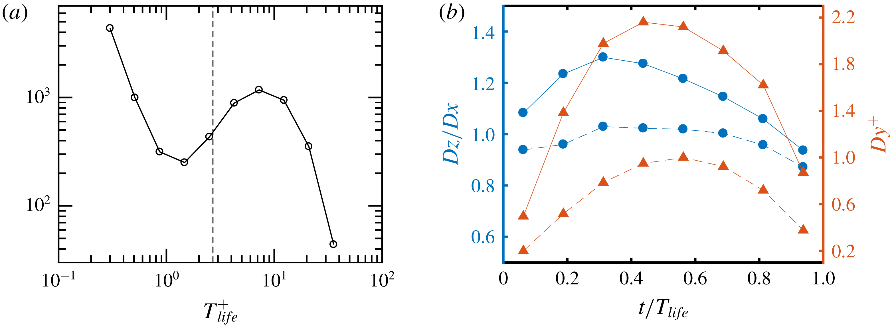
of the total backflow volume. For this reason, we will discard objects that split from and/or merged into other objects in the rest of this study, and look at the properties of the remaining 9800 objects with lifetimes distributed as shown on figure 2(a).
(a) Histogram of the lifetimes of backflow objects. The vertical broken line shows the minimum lifetime
 $T_{life}^{^{+}}=2.4$
of accepted objects in our statistical analyses. (b) Evolution of
 $Dz/Dx$
(circles) and
 $Dy^{+}$
(triangles) during different stages in the life of a backflow event.
 $2.4\leqslant T_{life}^{+}<19.2$
(broken lines) and
 $19.2\geqslant T_{life}^{+}$
(solid lines).

Long-living objects on figure 2(a) have lifetimes distributed similarly to log-normal. For shorter lifetimes, the probability density function exhibits an unphysical increase in probability, which we identify as a sign of events for which the temporal resolution is insufficient. The shortest lifetime that can be identified is given by those objects tracked for only two consecutive time steps of our
 $Re950TR$
sequence:
 $T_{life}^{^{+}}=0.3$
. The broken line on figure 2(a) shows the minimum lifetime
 $T_{life}^{^{+}}=2.4$
which we will accept in the remaining analysis. The removal of objects living less than this minimum lifetime conserves
 $94\,\%$
of the initial backflow volume, yet it brings their number down to approximately 3800 structures. They will constitute our sample set of dynamical events for the statistical analyses in the remainder of the paper. We note in passing that out of the approximately 6000 short-lived objects removed,
 $44\,\%$
never reached a size larger than a single grid cell in
 $x$
and
 $z$
.
5.2 Mean velocity
We study the mean velocity of the backflow objects by computing, for each object, the ratio between the total covered streamwise distance and its lifetime. Averaging this value over all objects, we find a mean velocity
 $u_{m}^{+}=9.4\pm 0.07$
, so that we are tracking objects of upstream velocity that convect downstream with the mean velocity corresponding to that of the mean flow at
 $y^{+}\approx 12$
. Cardesa et al. (Reference Cardesa, Monty, Soria and Chong2014) reported that critical points in the wall shear stress travel at a mean velocity of
 $9.5^{+}$
in the streamwise direction. The agreement between the two is to be expected, since backflow regions above the wall and critical points in the field of wall shear stress are closely related. Our finding for
 $u_{m}$
agrees well with del Álamo & Jiménez (Reference del Álamo and Jiménez2009), who report convection velocities of small-scale streamwise velocity right above the wall in the range
 $8^{+}-10^{+}$
, depending on the exact choice of spanwise and streamwise length scales kept in their averaging. That result is found to hold in the range
 $185\leqslant Re_{\unicode[STIX]{x1D70F}}\leqslant 1901$
, so we expect backflow regions to convect at the same mean speed within those Reynolds numbers.
5.3 Lifetime effects on the size of backflow objects
We split the lifetime of each structure into eight equal fractions, providing eight temporal bins on which we compute averages that map to different stages in the life of an object. More specifically, we compute
 $Dz/Dx$
and
 $Dy^{+}$
in the middle of each such temporal bin for every structure. By averaging over all structures but for a fixed life stage, we obtain the mean
 $Dz/Dx$
and
 $Dy^{+}$
that correspond to that life stage. We repeat the averaging for the remaining seven life stages, and obtain the mean values of
 $Dz/Dx$
and
 $Dy^{+}$
subject to being towards the youth, midlife or death of a backflow object, in a life stage conditional analysis similar to that of Cardesa, Vela-Martín & Jiménez (Reference Cardesa, Vela-Martín and Jiménez2017).
We show on figure 2(b) the mean
 $Dz/Dx$
and
 $Dy^{+}$
at each of the eight life stages considered. The average is computed separately for objects with lifetimes in the range
 $2.4\leqslant T_{life}^{+}<19.2$
and
 $19.2\geqslant T_{life}^{+}$
. It is revealing to see that the tendency of backflow objects towards a greater elongation in the spanwise over the streamwise direction, which was discussed in § 4 based on figure 1(b), is a feature of longer-lived objects. Backflow structures with lifetimes in the range
 $2.4\leqslant T_{life}^{+}<19.2$
appear to remain closer to circular. Similarly, longer-lived structures reach greater heights than short-lived ones – a fact that is perhaps less surprising but which figure 2(b) quantifies with a factor of more than twice the maximum mean height for
 $19.2\geqslant T_{life}^{+}$
over
 $2.4\leqslant T_{life}^{+}<19.2$
.
5.4 Mean large-scale dynamics around backflow events
We average the spanwise and wall-normal vorticity (
 $\unicode[STIX]{x1D714}_{z}$
and
 $\unicode[STIX]{x1D714}_{y}$
) in a box of size
 $(dx^{+},dy^{+},dz^{+})=(650,80,650)$
conditioned to the presence of a backflow structure in the middle of the bottom side of the box. Again, we split the lifetime of the structure into eight equal fractions, obtaining the mean
 $\unicode[STIX]{x1D714}_{z}$
and
 $\unicode[STIX]{x1D714}_{y}$
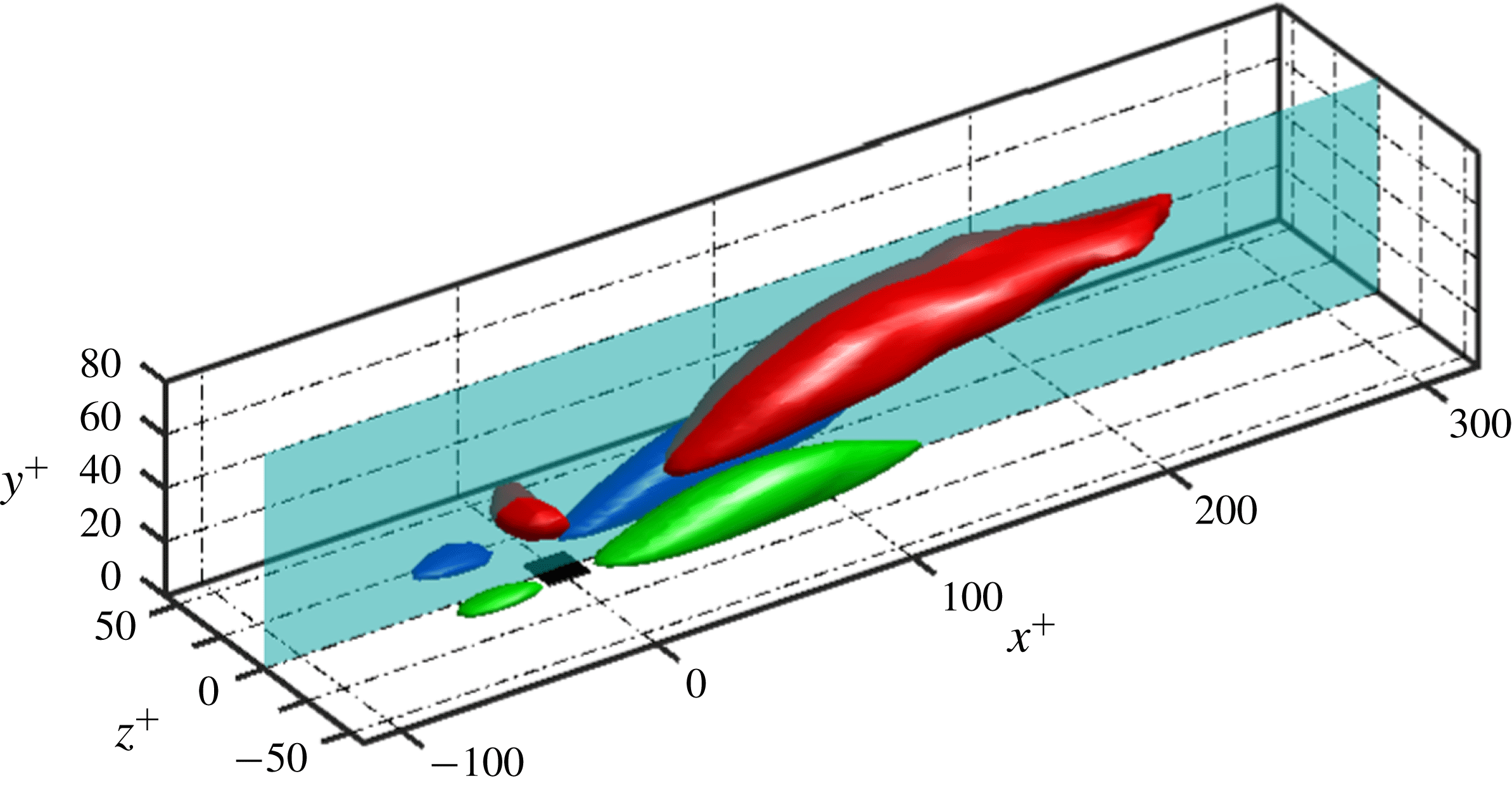
for different stages in the life of backflow events. We augment the temporal bins by three ‘eighths’ before the birth and after the death in order to uncover the average dynamical pattern leading to the formation and following the disappearance of the backflow events. Figure 3 shows data averaged during the first eighth in the life of a backflow object. On average, the conditional
 $\unicode[STIX]{x1D714}_{y}$
(in green and blue) leaves a spanwise-symmetric pattern around the backflow structure, with strong intense regions both downstream and upstream of the structure. We label as strong
 $\unicode[STIX]{x1D714}_{y}$
those areas above half of the maximum (blue) or below half the minimum (green) conditional mean. On average,
 $\unicode[STIX]{x1D714}_{y}$
should be zero, yet the conditional mean
 $\unicode[STIX]{x1D714}_{y}$
leads to extrema of
 $\pm 0.22^{+}$
found within the blue and green structures on figure 3. Note that on average, a backflow object is bounded by a box of dimensions as those seen in black at the origin of the axes on figure 3. For this reason, the visible footprint of the strong conditional
 $\unicode[STIX]{x1D714}_{y}$
extends far downstream when considering the typical size of a backflow structure. The conditionally averaged
 $\unicode[STIX]{x1D714}_{z}$
on figure 3 not only confirms the streamwise extent of the footprint of the backflow region, but also the height up to which a backflow event is correlated with a larger-scale event in
 $\unicode[STIX]{x1D714}_{z}$
. Lenaers et al. (Reference Lenaers, Li, Brethouwer, Schlatter and Örlü2012) found that the structure above a backflow event resembles an oblique vortex according to their observation based on visual inspection of individual snapshots. This is not inconsistent with our symmetric result, which is found after averaging.
 $\unicode[STIX]{x1D714}_{z}$
(red),
 $\unicode[STIX]{x1D714}_{y}>0$
(blue) and
 $\unicode[STIX]{x1D714}_{y}<0$
(green) conditioned to the first eighth of the life of a negative backflow region. The red iso-surface corresponds to twice the unconditional mean
 $\unicode[STIX]{x1D714}_{z}$
, while blue and green correspond to half of the maximum and minimum conditional
 $\unicode[STIX]{x1D714}_{y}$
, respectively. The
 $(x,y)$
plane at
 $z^{+}=0$
is the one on which results of figure 4 are plotted. The black square at the origin has the mean size of the bounding box of a backflow event during the first eighth of its life:
 $(21,1,22)$
in
 $(x^{+},y^{+},z^{+})$
.

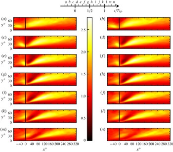
To visualize the mean temporal dynamics, we show on figure 4 the conditionally averaged
 $\unicode[STIX]{x1D714}_{z}$
projected on the
 $(x,y)$
plane of figure 3 at
 $z=0$
. This is done for all the temporal bins described above – see the temporal legend at the top of figure 4. Values are normalized with respect to the unconditional
 $y$
-dependent mean of
 $\unicode[STIX]{x1D714}_{z}$
. The sequence starts with a layer of above-average
 $\unicode[STIX]{x1D714}_{z}$
extending for approximately
 $300^{+}$
in the streamwise direction. Downstream from where the backflow event will appear (at
 $x^{+}=0$
on figure 4), the layer is tilted upwards and is longer than upstream of
 $x^{+}=0$
, where it is more localized. The events that follow can be summarized as a region of below-average mean
 $\unicode[STIX]{x1D714}_{z}$
landing on the shear layer, splitting it in two while intensifying it. The appearance of the backflow object in snapshot (
 $d$
) coincides with the layer of high
 $\unicode[STIX]{x1D714}_{z}$
being pushed against the wall. The intensification of
 $\unicode[STIX]{x1D714}_{z}$
upstream is shorter-lived (snapshots (
 $a$
) to (
 $e$
)) than that of the shear layer downstream (snapshots (
 $a$
) to (
 $k$
)) from the object. Snapshots (
 $d$
) to (
 $k$
) show how a thin high-
 $\unicode[STIX]{x1D714}_{z}$
layer is found below
 $y^{+}=15$
. Between snapshots (
 $d$
) and (
 $i$
), this thin layer connects the regions of high
 $\unicode[STIX]{x1D714}_{z}$
upstream and downstream from the backflow object. After snapshot (
 $i$
), the smaller shear layer upstream disconnects from the shear layer downstream as the former moves away from the wall and decays in intensity. After snapshot (
 $k$
), there is a clear trend towards the loss of coherence and the recovery of the unconditional mean
 $\unicode[STIX]{x1D714}_{z}$
. Before the birth, it is interesting to note that snapshot (
 $a$
) shows an elongated region of low
 $\unicode[STIX]{x1D714}_{z}$
below
 $y^{+}=15$
, which can be considered as a precursor state – in a statistical sense – to the appearance of the backflow event. Within this layer, the conditional mean
 $\unicode[STIX]{x1D714}_{z}$
is lower than the unconditional mean, but not of opposite sign. Opposite sign
 $\unicode[STIX]{x1D714}_{z}$
only appears during the life of the backflow region, and inside such few grid cells it is not apparent on figure 4. Backflow is linked to the thin layer of high conditional
 $\unicode[STIX]{x1D714}_{z}$
approaching the wall, yet remaining above low – and opposite sign –
 $\unicode[STIX]{x1D714}_{z}$
immediately above the wall.
6 Conclusions
Mean
 $\unicode[STIX]{x1D714}_{z}$
conditioned to a backflow event located at
 $x^{+}=\,0$
, normalized by the y-dependent unconditional mean of
 $\unicode[STIX]{x1D714}_{z}$
. The chosen plane corresponds to the
 $(x^{+},y^{+},z^{+}=\,0)$
slice shown on figure 3. Each field shows the average conditioned to different periods defined with respect to the life of the backflow event, which are labelled according to the linear key at the top of this figure. For instance, the field with label (d) corresponds to the average
 $\unicode[STIX]{x1D714}_{z}$
conditioned to being in the middle of the first eighth of the lifetime of a backflow event, while fields labelled (a) and (n) are conditioned to the third eighth before the birth and after the death of the backflow event, respectively. The box inside which the conditional average is taken remains fixed to the wall at the position of birth and death for fields (a–c) and (l–n), respectively. This explains the apparent streamwise drift of the conditional
 $\unicode[STIX]{x1D714}_{z}$
fields in (a–c) and (l–n).

Our findings show that the increase in the volume fraction of backflow for a given wall distance occurs together with an increase in the number of backflow structures per surface area – in wall units. These structures, although flat and circular on the average, are more elongated in the spanwise direction when above two wall units in height. The analysis of the evolution of individual backflow objects reveals that their height and spanwise elongation increase with their lifetime, and that on the average they advect downstream with a mean velocity
 $u_{m}^{+}=9.4\pm 0.07$
. The sequence of events described in our conditional dynamical analysis evidences the link between backflow regions in the viscous sublayer and the
 $Re_{\unicode[STIX]{x1D70F}}$
-dependent dynamics of much larger scales further away from the wall. It is this interaction which explains, for instance, the increase of backflow objects per surface area
 $n_{A}$
(in wall units) with increasing
 $Re_{\unicode[STIX]{x1D70F}}$
. Once the backflow objects are formed, their size could well be governed by viscosity only, implying a collapse of size distributions in wall units across Reynolds numbers. The contours on figure 1(b–d) support this idea, even though sample sizes for the largest objects prevent us from being conclusive. Backflow objects exhibit negligible interaction between them, with most of them experiencing no splits from or mergers with other backflow objects. We expect this situation observed in channel flows to be rather different in adverse pressure gradient turbulent boundary layers, or on the curved wall of aerofoils with varying degrees of flow separation. The tracking of backflow regions in such simulations would be a natural extension to the present study.
Acknowledgements
This research was funded in part by the Multiflow project of the European Research Council and the Australian government through the Australian Research Council.