1 Introduction
Intense sediment transport occurs when the flow-induced bed shear stress is sufficiently strong to wash out bed forms and to mobilize a thick and dense layer of particles on the top of the sediment bed. In the hydraulic literature, this regime is usually referred to as sheet-flow regime or upper plane-bed stage. Provided that the particle settling velocity
 $w_{s}$
is lower than or of the order of the turbulent velocity scale
 $u_{\ast }$
, a fraction of the mobilized sediment is transported in suspension at a much lower concentration than in the bed-load layer. The Shields number
 $\unicode[STIX]{x1D703}$
and the suspension number
 $S$
are the two dimensionless numbers that control intense sediment transport regimes (Sumer et al.
Reference Sumer, Kozakiewicz, Fredsøe and Deigaard1996). The Shields number is the ratio between the force exerted by the fluid on a particle of the bed and the apparent weight of a single immersed particle. The suspension number characterizes the competition between the particle inertia represented by its settling velocity and the magnitude of the turbulent velocity fluctuations represented by the friction velocity. The present paper focuses on uniform, steady and fully turbulent flows over mobile beds of well-sorted particles, in which the bed slope
 $S_{0}$
is sufficiently low to neglect the body force acting on the particles.
The pioneering work of Bagnold (Reference Bagnold1956) suggested that both granular interactions and turbulent processes constitute key mechanisms of momentum diffusion in the near-bed region. The granular shear stress has been modelled via kinetic theory of granular flow (Hanes & Bowen Reference Hanes and Bowen1985; Jenkins & Hanes Reference Jenkins and Hanes1998; Capart & Fraccarollo Reference Capart and Fraccarollo2011) or via dense granular flow rheology (Revil-Baudard & Chauchat Reference Revil-Baudard and Chauchat2013). The turbulent shear stress has been modelled using the mixing length models (Nnadi & Wilson Reference Nnadi and Wilson1992; Jenkins & Hanes Reference Jenkins and Hanes1998; Revil-Baudard & Chauchat Reference Revil-Baudard and Chauchat2013) or more refined
 $k{-}\unicode[STIX]{x1D716}$
models (Hsu, Jenkins & Liu Reference Hsu, Jenkins and Liu2004), modified to account for the feedback of the mobile sediments on the fluid turbulence. However, the extreme difficulty to measure both velocity and concentration across the near-mobile-bed region has strongly limited our understanding of the interactions between the turbulent fluid flow and the mobile bed (Castro-Orgaz et al.
Reference Castro-Orgaz, Giráldez, Mateos and Dey2012, pp. 1–2). The poor accuracy in the numerical prediction of sediment transport rates (Recking Reference Recking2010) and associated bed morphology under flood conditions is therefore not surprising. Another scientific bottleneck resides in the prediction of the concentration profile in the diluted region of the flow in which the particles are suspended by the turbulent fluctuations of the wall-normal fluid velocity (Greimann, Muste & Holly Jr. Reference Greimann, Muste and Holly1999). It is now well-accepted that the model presented by Rouse (Reference Rouse1937), which is based on a balance between the downward gravity-driven settling flux and the upward turbulent dispersion flux, allows the suspended concentration profiles to be accurately predicted. However, this physically-based model induces a tunable parameter, the turbulent Schmidt number, ratio between the momentum and concentration diffusivities (
 $\unicode[STIX]{x1D70E}_{s}=\unicode[STIX]{x1D716}_{m}/\unicode[STIX]{x1D716}_{p}$
). The value of this parameter is subject to open discussion in the literature (e.g. Nielsen & Teakle Reference Nielsen and Teakle2004).
In Revil-Baudard et al. (Reference Revil-Baudard, Chauchat, Hurther and Barraud2015), the time-resolved vertical profiles of concentration, velocity and bed interface revealed a modification of the von Kármán parameter and the Schmidt number. Furthermore, the times series plots showed a qualitative correlation between the bed-interface variations and the presence of turbulent large-scale coherent structures identified as ejection and sweep events. For the present paper, a new dataset has been collected with a doubled measurement resolution under a stronger forcing condition. It is used together with that presented in Revil-Baudard et al. (Reference Revil-Baudard, Chauchat, Hurther and Barraud2015) to investigate the interactions between the turbulent flow and the mobile bed in intense particle-laden shear flows. The effect of the bed variability on the turbulent quantities is first discussed and a statistical interpretation for the low values of the von Kármán parameter and the Schmidt number observed in previous studies (e.g. Vanoni Reference Vanoni1946; Best et al. Reference Best, Bennett, Bridge and Leeder1997; Nielsen & Teakle Reference Nielsen and Teakle2004) is proposed. The experimental set-up, instrumentation and signal processing are introduced in § 2. The results are presented and analysed in § 3 and the main insights are summarized in § 4.
2 Methodology
2.1 Experimental set-up
The new set of data is obtained from an experiment carried out in the LEGI/ENSE3 tilting flume using the same protocol as in Revil-Baudard et al. (Reference Revil-Baudard, Chauchat, Hurther and Barraud2015). The same acoustic instrumentation (ACVP technology) is also utilized for the new experiment. This instrumentation measures the co-located streamwise (
 $u$
), wall-normal (
 $w$
), velocities and the particle volumetric concentration (
 $\unicode[STIX]{x1D719}$
) over a vertical profile extending from the undisturbed bed level (
 $z=0$
) to the top of the free surface (
 $z=H_{f}$
). The difference with Revil-Baudard et al. (Reference Revil-Baudard, Chauchat, Hurther and Barraud2015) lies in the vertical resolution of the ACVP measurements which has been doubled and is equal to
 $\unicode[STIX]{x0394}z=1.5$
mm. The acoustic bed interface tracking (ABIT) of Hurther & Thorne (Reference Hurther and Thorne2011) is used here for the localization of the bed interface defined as the vertical position of the non-moving sediments. Time tracking of this position allows a bed-intermittency function to be evaluated, as defined in the next section. The sampling frequency is
 $78$
,
 $4.8$
and
 $7.8$
Hz for the velocity, concentration and bed-interface measurements, respectively. The free-surface level is measured using an acoustic limnimeter.
Experimental parameters. Particle diameter (
 $d_{p}$
), settling velocity (
 $w_{s}$
), friction velocity (
 $u_{\ast }$
), Shields number (
 $\unicode[STIX]{x1D703}=\unicode[STIX]{x1D70C}_{f}u_{\ast }^{2}/\unicode[STIX]{x0394}\unicode[STIX]{x1D70C}gd_{p}$
), suspension number (
 $S=w_{s}/u_{\ast }$
), dimensionless solid load (
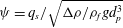 $\unicode[STIX]{x1D713}=q_{s}/\sqrt{\unicode[STIX]{x0394}\unicode[STIX]{x1D70C}/\unicode[STIX]{x1D70C}_{f}gd_{p}^{3}}$
), water flow rate (
 $Q_{f}$
), flume slope (
 $S_{0}$
), mean bulk velocity (
 $U$
), water depth (
 $H_{f}$
), bulk Reynolds number (
 $Re_{b}=UH_{f}/\unicode[STIX]{x1D708}$
), von Kármán parameter (
 $\unicode[STIX]{x1D705}$
), zero-plane level (
 $z_{d}$
), mean bed-interface position (
 $z_{b}$
) where
 $q_{s}$
is the solid load per unit width,
 $\unicode[STIX]{x1D70C}_{f}=1000~\text{kg}~\text{m}^{-3}$
,
 $\unicode[STIX]{x0394}\unicode[STIX]{x1D70C}=192~\text{kg}~\text{m}^{-3}$
,
 $g=9.81~\text{m}~\text{s}^{-2}$
and
 $\unicode[STIX]{x1D708}=10^{-6}~\text{m}^{2}~\text{s}^{-1}$
.

The measurements of three experiments are analysed here. Two are intense sediment transport flows and one is a clear-water flow over a fixed rough-wall constituted of the same particles as those used for the sediment transport experiments. The first mobile-bed run is denoted as MB
 $_{1}$
in the following and corresponds to that presented in Revil-Baudard et al. (Reference Revil-Baudard, Chauchat, Hurther and Barraud2015). The second mobile-bed experiment (MB
 $_{2}$
) involved the same particles as MB
 $_{1}$
and corresponds to the more intense sediment transport regime with twice the measurement resolution. The runs have been repeated
 $N=11$
times for MB
 $_{1}$
and
 $N=12$
times for MB
 $_{2}$
in order to perform ensemble averaging as described in Revil-Baudard et al. (Reference Revil-Baudard, Chauchat, Hurther and Barraud2015). The clear-water flow run (CW) has been performed under similar forcing conditions as the sediment transport experiments. This provides a reference to investigate the interactions between the turbulent flow and the mobile bed. The experimental parameters are presented in table 1.
2.2 Data processing methods
As described in Revil-Baudard et al. (Reference Revil-Baudard, Chauchat, Hurther and Barraud2015), an ensemble-averaging experimental protocol has been applied to investigate the sediment transport processes under steady uniform open-channel flow conditions in the absence of a sediment recirculating facility. First, the time period
 $t\in [t_{1}-t_{2}]$
for which the flow is uniform is identified based on the vertical linearity of the mean turbulent shear-stress profile. Then, the local and instantaneous velocity, concentration and sediment flux measurements are averaged temporally over
 $\unicode[STIX]{x0394}t=t_{2}-t_{1}$
and over the
 $N$
realizations of the same experiment to obtain statistically converged velocities, concentration and sediment flux profiles,
 $$\begin{eqnarray}\displaystyle \langle A\rangle ^{S}(z)=\frac{1}{N}\mathop{\sum }_{i=1}^{N}\left(\frac{1}{\unicode[STIX]{x0394}t}\int _{t_{1}}^{t_{2}}A_{i}(t,z)\,\text{d}t\right), & & \displaystyle\end{eqnarray}$$
in which
 $\unicode[STIX]{x0394}t=6$
s. The operator
 $\langle -\rangle ^{S}$
refers to an ensemble average (over the number of repeated experiments) of the temporal superficial mean of quantity
 $A$
. In the following, the word temporal is omitted for brevity in the terminologies intrinsic and superficial averages. The results in Revil-Baudard et al. (Reference Revil-Baudard, Chauchat, Hurther and Barraud2015) revealed an important temporal bed-level variability in the near-bed region. Consequently, the temporal bed-intermittency function,
 $\unicode[STIX]{x1D719}_{I}(z)$
, defined as the time fraction for which the mixture velocity (i.e. of the fluid or of the particle) is non-zero at a given vertical position
 $z$
, is introduced to characterize this temporal bed-level variability. It reads as follows:
 $$\begin{eqnarray}\displaystyle \unicode[STIX]{x1D719}_{I}(z)=\frac{\displaystyle \mathop{\sum }_{i=1}^{N}\unicode[STIX]{x0394}t_{i}^{\unicode[STIX]{x1D719}}(z)}{N\times \unicode[STIX]{x0394}t}, & & \displaystyle\end{eqnarray}$$
where
 $\unicode[STIX]{x0394}t_{i}^{\unicode[STIX]{x1D719}}(z)$
represents the time duration of realization
 $i$
for which mixture velocity is non-zero within the time interval
 $\unicode[STIX]{x0394}t=t_{2}-t_{1}$
at a vertical location
 $z$
. It follows that
 $\unicode[STIX]{x1D719}_{I}(z)=0$
in the undisturbed bed region and
 $\unicode[STIX]{x1D719}_{I}(z)=1$
above the bed-level variation range. Under mobile-bed conditions (i.e. when the local bed level is time dependent), the temporal bed-intermittency function is similar to the spatial roughness geometry function (defined as the ratio between the area occupied by the fluid divided by the total area, in the double averaging method) if the bed-level fluctuation is a random ergodic process. As in the doubled averaging method, the intrinsic average of
 $\langle A\rangle ^{I}$
is related to the superficial ones (Nikora et al.
Reference Nikora, Goring, Mcewan and Griffiths2001, Reference Nikora, Ballio, Coleman and Pokrajac2013; Radice & Ballio Reference Radice and Ballio2008; Mignot, Barthélémy & Hurther Reference Mignot, Barthélémy and Hurther2009a
) as
 $$\begin{eqnarray}\displaystyle \langle A\rangle ^{S}(z)=\unicode[STIX]{x1D719}_{I}(z)\langle A\rangle ^{I}(z). & & \displaystyle\end{eqnarray}$$
Unlike the superficial quantities, non-moving events are not considered in the intrinsic quantities. Consistently, above the region of bed-level variation, where
 $\unicode[STIX]{x1D719}_{I}=1$
, the superficial and intrinsic averages are strictly identical.
The local and instantaneous fluctuations of velocity and concentration for each realization read
 $$\begin{eqnarray}\displaystyle A_{i}^{\prime k}(t,z)=A_{i}^{k}(t,z)-\langle A\rangle ^{k}(z), & & \displaystyle\end{eqnarray}$$
where the superscript
 $k$
stands either for the intrinsic
 $I$
or the superficial
 $S$
quantities. Here
 $A_{i}^{S}(t,z)$
corresponds to the entire time series of velocities and concentration while
 $A_{i}^{I}(t,z)$
is restricted to measurements for which the velocity is non-zero.
The mean Reynolds shear stresses
 $\langle u^{\prime }w^{\prime }\rangle ^{k}(z)$
are evaluated as
 $$\begin{eqnarray}\displaystyle \langle u^{\prime }w^{\prime }\rangle ^{k}(z)=\frac{1}{N}\mathop{\sum }_{i=1}^{N}\left(\frac{1}{\unicode[STIX]{x0394}t}\int _{t_{1}}^{t_{2}}u_{i}^{\prime k}(t,z)w_{i}^{\prime k}(t,z)\,\text{d}t\right). & & \displaystyle\end{eqnarray}$$
The method proposed by Garbini, Forster & Jorgensen (Reference Garbini, Forster and Jorgensen1982) is employed to remove the Doppler noise contribution from the root mean square (r.m.s.) of the velocity fluctuations:
 $$\begin{eqnarray}\displaystyle u_{rms}^{k}(z)=\sqrt{\langle u^{\prime k}(z,t)u^{\prime k}(z+\unicode[STIX]{x0394}z,t)\rangle },\quad w_{rms}^{k}(z)=\sqrt{\langle w^{\prime k}(z,t)w^{\prime k}(z+\unicode[STIX]{x0394}z,t)\rangle }.\qquad & & \displaystyle\end{eqnarray}$$
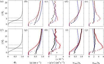
Intermittency functions (a,f), intrinsic (
 $\star$
) and superficial (▵) velocity profiles (b,g), shear-stress profiles (c,h), wall normal (d,i) and streamwise (e,j) r.m.s. of velocity fluctuations for the runs MB
 $_{1}$
(a–e) and MB
 $_{2}$
(f–j). The solid lines on panels (a,f) represent the mean position of the measured fixed bed-interface, plus and minus the associated standard deviation (- - -). The results from the CW run (
 $\boldsymbol{\cdot }$
) are also presented for comparison.

3 Results and discussion
3.1 Superficial versus intrinsic averaging
Figure 1 presents the bed-intermittency function and the profiles of velocity, Reynolds shear stress, streamwise and wall-normal turbulence intensities obtained using the superficial and intrinsic averaging methods for runs MB
 $_{1}$
(a–e) and MB
 $_{2}$
(f–j). The mean profiles obtained for the clear-water case are also shown for comparison. It can be seen that the bed-intermittency functions present qualitatively the same ‘S shape’ for both runs (figure 1
a,f). The average position of the fixed bed-interface is located at
 $z_{b}/d_{p}=3.5$
and at
 $z_{b}/d_{p}=4.2$
for runs MB
 $_{1}$
and MB
 $_{2}$
, respectively. The associated standard deviations of the bed-interface position are
 $z_{rms}/d_{p}=2.3$
and
 $z_{rms}/d_{p}=3.0$
for runs MB
 $_{1}$
and MB
 $_{2}$
, respectively. These values confirm the strong dynamic of the bed-interface as they are comparable with the thickness of the bed-load layer (
 $\unicode[STIX]{x1D6FF}_{s}\approx 5d_{p}$
) evaluated from a concentration criteria (
 $\unicode[STIX]{x1D719}>0.08$
) (Hsu, Jenkins & Liu Reference Hsu, Jenkins and Liu2003).
Figure 1(b,g) presents the superficial and intrinsic velocity profiles. It can be observed that the bed variability has a significant influence on the velocity profile up to
 $z/d_{p}\approx 10$
for MB
 $_{1}$
and up to
 $z/d_{p}\approx 15$
for MB
 $_{2}$
. Due to the increasing number of zero-velocity events in the vicinity of the bed, the superficial velocity values are lower than the intrinsic values. The clear inflection observed on the superficial velocity profiles cannot be seen on the intrinsic velocity profiles. One can conclude that the S shape observed in the superficial velocity profiles is imposed by the bed-intermittency function.
The intrinsic and superficial turbulent shear-stress profiles are represented in figure 1(c,h). The superficial shear-stress profile presents significantly larger values than the intrinsic profile in the near-bed region for both MB
 $_{1}$
and MB
 $_{2}$
runs. In other words, the correlation rate between streamwise and wall-normal velocity fluctuations is higher when accounting for the bed intermittency. As the correlation
 $\langle u^{\prime }w^{\prime }\rangle$
can be interpreted as a turbulent momentum flux, it results that the bed intermittency induces an additional shear stress.
The wall-normal and streamwise turbulence intensities are shown in figure 1(d,i) and (e,j), respectively. It can be seen that for
 $z/d_{p}>15$
, the normalized wall-normal and streamwise turbulence intensities are consistent with the scaling commonly found in the literature for standard turbulent boundary layers:
 $w_{rms}\approx u_{\ast }$
and
 $u_{rms}\approx 2u_{\ast }$
(Nezu & Nakagava Reference Nezu and Nakagava1993). It is also observed that for both experiments the intrinsic wall-normal turbulence intensity is slightly greater than the superficial one in the near-bed region. The streamwise intrinsic turbulence intensity on the other hand is significantly lower than the superficial one. This implies that the bed-variability is responsible for more than half of the streamwise velocity fluctuation intensity near the maximum (
 $z/d_{p}\approx 5$
). It is noteworthy that in the region
 $10<z/d_{p}<15$
, the Reynolds shear stresses present similar values for the three cases (figure 1
c,h), however the streamwise and wall-normal turbulence intensities are clearly increased in the presence of sediment transport (figure 1
d,i,e,j). This point will be discussed in detail in § 3.3.
3.2 Logarithmic law and Rouse profile
The logarithmic law allows to predict the velocity profile in the overlapping layer between the outer layer, scaling with the flow depth, and the inner layer scaling with the roughness length scale (e.g. Jiménez Reference Jiménez2004). In the overlapping layer the relevant local length scale becomes the wall distance. It results that the local turbulent viscosity scales as
 $\unicode[STIX]{x1D716}_{m}\propto l_{m}^{2}\,\text{d}u/\text{d}z$
, where
 $l_{m}(z)=\unicode[STIX]{x1D705}(z-z_{d})$
is the mixing length. The von Kármán parameter
 $\unicode[STIX]{x1D705}$
presents a universal value (
 $\unicode[STIX]{x1D705}\approx 0.4$
) for single-phase turbulent boundary layers. The origin of the mixing length,
 $z_{d}$
, is also called the ‘zero-plane level’ of the law of the wall. The resulting logarithmic law,
 $$\begin{eqnarray}\displaystyle u(z)=\frac{u_{\ast }}{\unicode[STIX]{x1D705}}\text{ln}\left(\frac{z-z_{d}}{z_{0}}\right), & & \displaystyle\end{eqnarray}$$
has been fitted on the present superficial velocity profiles to obtain the values of
 $\unicode[STIX]{x1D705}$
and
 $z_{d}$
. To do so, the bed friction velocity
 $u_{\ast }$
is evaluated independently from the linear extrapolation of the measured Reynolds shear-stress at
 $z=0$
(see table 1) and the roughness length
 $z_{0}$
is obtained using a measured boundary condition,
 $U(z_{A})=U_{A}$
, leading to
 $z_{0}=(z_{A}-z_{d})/\text{e}^{\unicode[STIX]{x1D705}U_{A}/u_{\ast }}$
. This methodology is used to avoid a three-parameter fit with a single equation. The vertical fitting range is selected to maximize the regression coefficient
 $R_{u}^{2}$
. It has been verified that the results do not depend on the choice of
 $z_{A}$
provided that it is located within the vertical fitting range. The resulting fitted parameters (
 $\unicode[STIX]{x1D705},z_{d}$
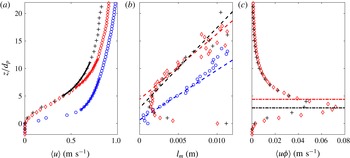
) are presented in table 1. Figure 2(a) presents the comparison between the superficial velocity profiles and the associated logarithmic fits. The very high values of the obtained regression coefficients (
 $R_{u}^{2}>0.999$
) suggest that the logarithmic law is an appropriate model for the velocity profiles over a given vertical range, provided that
 $\unicode[STIX]{x1D705}$
,
 $z_{d}$
,
 $u_{\ast }$
and
 $z_{0}$
(or a particular velocity value
 $U_{A}(z_{A})$
) are known. Both
 $\unicode[STIX]{x1D705}$
and
 $u_{\ast }$
appear only in the proportionality factor of equation (3.1), implying that the uncertainty in
 $\unicode[STIX]{x1D705}$
is directly related to the uncertainty in
 $u_{\ast }$
(
 ${<}20\,\%$
). Despite this uncertainty, the value of
 $\unicode[STIX]{x1D705}$
is shown to be significantly affected by the presence of the mobile sediment bed in the turbulent boundary layer, as previously observed and discussed in the literature (e.g. Vanoni Reference Vanoni1946; Gaudio, Miglio & Dey Reference Gaudio, Miglio and Dey2010; Castro-Orgaz et al.
Reference Castro-Orgaz, Giráldez, Mateos and Dey2012).
Assuming a constant shear stress in the log layer, one can also evaluate the mixing length profile as
 $l_{m}=u_{\ast }/|\text{d}u/\text{d}z|$
. Figure 2(b) presents the resulting mixing length (markers) compared with the formulation
 $l_{m}(z)=\unicode[STIX]{x1D705}(z-z_{d})$
(dashed lines), in which
 $\unicode[STIX]{x1D705}$
and
 $z_{d}$
are obtained from the fit of the velocity profile. Very good agreement is observed, especially over the vertical range employed for the logarithmic fit. For the clear-water experiment, the zero-plane level
 $z_{d}$
is found to be located close to the position at which the mean streamwise velocity vanishes. In the mobile-bed experiments,
 $z_{d}$
is located higher, close to the average position of the bed interface
 $z_{b}$
(table 1).
According to Nikora et al. (Reference Nikora, Koll, Mclean, Dittrich and Aberle2002) and Pokrajac, McEwan & Nikora (Reference Pokrajac, Mcewan and Nikora2008), the zero-plane level corresponds to the average level of penetration of large-scale turbulent events. Furthermore, the visualization of the large-scale coherent structures in Revil-Baudard et al. (Reference Revil-Baudard, Chauchat, Hurther and Barraud2015) revealed a deep penetration into the sediment bed. The overlap of the zero-plane level and the average position of the bed interface confirms the existence of a strong coupling between the large-scale turbulent structures and the bed dynamics. Jackson (Reference Jackson1981) interpreted the zero-plane level
 $z_{d}$
as the effective level of the line of action for momentum extraction induced by the roughness elements. In bed-load flows, it implies that the parameter
 $z_{d}$
corresponds to the effective level at which the fluid momentum is transmitted from the large-scale turbulent eddies to the sediment particles. Figure 2(c) presents the average sediment flux for MB
 $_{1}$
and MB
 $_{2}$
and the corresponding zero-plane levels. They are found to be located in regions of high sediment flux. This indicates that momentum is directly transferred from the large-scale structures toward the solid phase to enhance sediment transport. This should be verified for higher Shields numbers though, for which the bed-load layer is thicker.
Velocity (a), mixing length (b) and sediment flux profiles (c) for MB
 $_{1}$
(
 $+$
), MB
 $_{2}$
(♢) and CW (○). The solid lines in (a) correspond to (3.1), the dashed lines in (b) correspond to
 $l_{m}(z)=\unicode[STIX]{x1D705}(z-z_{d})$
and the dot-dashed lines in (c) correspond to the zero-plane levels.

Two main features arise from the interpretation of the zero-plane level. First, from a mixture point of view, the proximity between the zero-plane level and the mean bed-interface position supports the existence of a strong correlation between the variation of the bed interface and the large-scale turbulent structures. This coupling results in a bed-variability-induced shear stress across the near-bed region (see figure 1 c,h). Second, from a two-phase point of view, the proximity between the zero-plane levels and the regions of maximum flux strongly suggests a direct transfer of momentum from the large-scale turbulent structures toward the dense mobile layer.
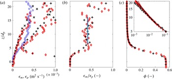
(a) Momentum (
 $\times$
, ▫, ○) and concentration (
 $+$
, ♢) diffusivities (3.2) and (3.3). (b) Ratio between momentum and concentration diffusivities. The vertical line corresponds to the Schmidt number value,
 $\unicode[STIX]{x1D70E}_{s}=0.4$
, represented over the vertical range on which it is evaluated. (c) Measured (markers) and fitted (solid line) concentration profiles (3.4) for MB
 $_{1}$
(
 $+$
,
 $\times$
), MB
 $_{2}$
(♢, ▫) and CW (○).

Assuming Fickian diffusion for momentum and concentration (Nielsen & Teakle Reference Nielsen and Teakle2004), the vertical momentum diffusivity, equal to the turbulent eddy viscosity, is evaluated as
 $$\begin{eqnarray}\displaystyle \unicode[STIX]{x1D716}_{m}=\frac{\langle u^{\prime }w^{\prime }\rangle ^{S}}{|\text{d}u/\text{d}z|}. & & \displaystyle\end{eqnarray}$$
Consistently, the particle (or concentration) diffusivity is
 $$\begin{eqnarray}\displaystyle \unicode[STIX]{x1D716}_{p}=\frac{\unicode[STIX]{x1D719}w_{s}}{|\text{d}\unicode[STIX]{x1D719}/\text{d}z|}, & & \displaystyle\end{eqnarray}$$
where it is assumed that the upward turbulent concentration flux
 $w^{\prime }\unicode[STIX]{x1D719}^{\prime }$
is balanced by a downward settling flux
 $\unicode[STIX]{x1D719}w_{s}$
. The corresponding profiles are presented in figure 3(a) for MB
 $_{1}$
, MB
 $_{2}$
and CW. It can be seen that in the logarithmic layer the momentum diffusivity is lower for mobile-bed experiments. This is consistent with the low values of the mixing length and of the von Kármán parameter (figure 2
a,b). It can also be seen in figure 3(a) that the concentration diffusivity
 $\unicode[STIX]{x1D716}_{p}$
is significantly higher than the momentum one
 $\unicode[STIX]{x1D716}_{m}$
for both sediment transport experiments. The ratio
 $\unicode[STIX]{x1D716}_{m}/\unicode[STIX]{x1D716}_{p}$
is presented in figure 3(b). A fairly constant value is observed for
 $6<z/d_{p}<16$
, corresponding to a Schmidt number value of
 $\unicode[STIX]{x1D70E}_{s}=0.4$
in both experiments. Following Revil-Baudard et al. (Reference Revil-Baudard, Chauchat, Hurther and Barraud2015), the concentration profile can be predicted theoretically using the Rouse formulation,
 $$\begin{eqnarray}\displaystyle \unicode[STIX]{x1D719}(z)=\unicode[STIX]{x1D719}_{r}\left(\frac{z-z_{d}}{z_{r}-z_{d}}\right)^{p}, & & \displaystyle\end{eqnarray}$$
where
 $p=-(\unicode[STIX]{x1D70E}_{s}w_{s}/\unicode[STIX]{x1D705}u_{\ast })$
is the Rouse number and
 $\unicode[STIX]{x1D719}_{r}=\unicode[STIX]{x1D719}(z_{r})$
is a measured reference concentration located at the lower boundary of the logarithmic layer (i.e. the first point of the vertical range employed for the log fit, see figure 2
a). Figure 3(c) compares the measured concentration profiles with the theoretical ones (3.4). The very good agreement obtained between the measurements and the Rouse profile confirms the validity of this formulation in the suspension layer provided that
 $u_{\ast }$
,
 $\unicode[STIX]{x1D705}$
,
 $\unicode[STIX]{x1D70E}_{s}$
,
 $z_{d}$
and a given reference concentration
 $\unicode[STIX]{x1D719}_{r}(z_{r})$
are known.
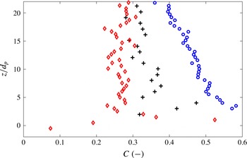
Correlation coefficients,
 $C=\langle u^{\prime }w^{\prime }\rangle ^{I}/u_{rms}^{I}w_{rms}^{I}$
, for MB
 $_{1}$
(
 $+$
), MB
 $_{2}$
(♢) and CW (○).

3.3 Turbulent correlation coefficient and quadrant dynamics
According to Greimann et al. (Reference Greimann, Muste and Holly1999), for example, the vertical dispersion of settling particles in a boundary layer is related to the diagonal terms of the Reynolds stress tensor, i.e. the vertical turbulent normal stress. Therefore, the ratio of the deviatoric component (linked with momentum diffusion) to the diagonal components characterizes the relative efficiency of momentum mixing to particle dispersion. The correlation coefficient,
 $$\begin{eqnarray}\displaystyle C=\frac{\langle u^{\prime }w^{\prime }\rangle ^{I}}{u_{rms}^{I}w_{rms}^{I}}, & & \displaystyle\end{eqnarray}$$
a proxy for this ratio, is plotted in figure 4. In the three experiments, the correlation coefficients present rather constant values in the upper part of the flow (
 $z/d_{p}\gtrsim 5$
). The clear-water flow value is in agreement with those reported in the literature for clear-water and atmospheric boundary layers (i.e.
 $C\approx 0.45$
) (Townsend Reference Townsend1976; Pope Reference Pope2000; Manes, Poggi & Ridolfi Reference Manes, Poggi and Ridolfi2011). The decrease of
 $C$
under mobile-bed flow conditions explains the low value of the Schmidt number. It is also consistent with the observations made from figure 1(c–e,h–j) in the upper part of the flow where the turbulent shear-stress values are similar for the three cases whereas the normal stresses are larger for the mobile-bed flow compared with the clear-water case. This effect was not observed in fully-resolved numerical simulation from Derksen (Reference Derksen2015) in which the fluid turbulence intensity is damped by the presence of particles at similar Shields number. The author also reports a drastic increase of particle velocity fluctuations for Shields number around 0.6. Keeping in mind that in the present experiments the measured velocity is the mixture one, fluid and particles, it is not impossible that Derksen’s results are consistent with the present experiments. Fluid–particle turbulent interactions in turbulent shear boundary layers is still an open problem and it is believed that eddy resolving simulations together with high resolution experimental measurements is the only way to obtain further insight. This will require further investigation in the future.
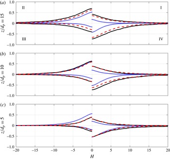
Quadrant threshold distribution
 $RSq(H)$
for MB
 $_{1}$
(——), MB
 $_{2}$
(- - -) and CW (
 $\cdot \,\cdot \,\cdot$
) at (a)
 $z/d_{p}=5$
, (b)
 $z/d_{p}=10$
and (c)
 $z/d_{p}=15$
.

To further investigate the reduction of the correlation coefficient shown in figure 4, an analysis of the Reynolds shear stress is carried out on the basis of the well-known quadrant threshold distributions (Lu & Willmarth Reference Lu and Willmarth1973; Nakagawa & Nezu Reference Nakagawa and Nezu1977; Raupach Reference Raupach1981; Niño & Garcia Reference Niño and Garcia1996; Hurther, Lemmin & Terray Reference Hurther, Lemmin and Terray2007; Mignot, Hurther & Barthélémy Reference Mignot, Hurther and Barthélémy2009b
). The quadrant threshold distribution
 $RSq(H)$
represents the relative contribution of the conditionally sampled velocity covariance
 $u^{\prime }w^{\prime }$
as a function of the threshold level
 $H$
and its orientation in the
 $(u^{\prime },w^{\prime })$
plane. As originally proposed by Lu & Willmarth (Reference Lu and Willmarth1973), the four quadrants are referred to as: outward interactions (
 $q=I$
with
 $u^{\prime }>0$
and
 $w^{\prime }>0$
), ejections (
 $q=II$
with
 $u^{\prime }<0$
and
 $w^{\prime }>0$
), inward interactions (
 $q=III$
with
 $u^{\prime }<0$
and
 $w^{\prime }<0$
) and sweeps (
 $q=IV$
with
 $u^{\prime }>0$
and
 $w^{\prime }<0$
). The quadrant threshold distribution is defined as
 $$\begin{eqnarray}\displaystyle \left.\begin{array}{@{}c@{}}RSq(z,H)=\langle \unicode[STIX]{x1D6FE}(z,t)D(\unicode[STIX]{x1D6FE})\rangle ^{I},\\ \unicode[STIX]{x1D6FE}(z,t)=u^{\prime }w^{\prime }(z,t)/u_{\ast }^{2},\\ D(\unicode[STIX]{x1D6FE})=1\quad \text{if }|\unicode[STIX]{x1D6FE}|>H\;\& \;u^{\prime }w^{\prime }\in q,\\ D(\unicode[STIX]{x1D6FE})=0\quad \text{otherwise}.\end{array}\right\} & & \displaystyle\end{eqnarray}$$
The quadrant distributions for the two mobile-bed and the clear-water cases are presented in figure 5 for the vertical positions
 $z/d_{p}=5$
,
 $z/d_{p}=10$
and
 $z/d_{p}=15$
. The quadrant threshold distributions for the clear-water flow case (dotted curves in figure 5) are in close agreement with the results found in the literature for high Reynolds number rough-bed flows (Nakagawa & Nezu Reference Nakagawa and Nezu1977; Raupach Reference Raupach1981; Hurther et al.
Reference Hurther, Lemmin and Terray2007). The contributions associated with ejection and sweep events are significantly higher than the contributions of inward and outward interactions. This explains the negative sign of the net mean Reynolds shear stress, i.e. when the contributions are added over the four quadrants for
 $H=0$
. This typical quadrant signature has been discussed in detail in the literature for clear-water shear flows under smooth and rough rigid-bed conditions (Nezu & Nakagava Reference Nezu and Nakagava1993). In particular, it can be seen in figure 5 that the ejection contribution is slightly higher than the sweep contribution at
 $z/d_{p}=15$
(i.e. above the log layer) and that this excess of ejection-induced shear stress vanishes with proximity to the rigid bed (here at
 $z/d_{p}=5$
for CW). As shown by Raupach (Reference Raupach1981) and synthesized by Nezu & Nakagava (Reference Nezu and Nakagava1993, p. 184, § 8.4), the increasing sweep-induced contribution near the rigid bed characterizes the existence of a roughness sublayer in which sweep-induced shear stress dominates over the ejection-induced contribution. A characteristic thickness for the roughness sublayer can be defined as the height of identical shear-stress contribution between ejections and sweeps. A value of
 $5d_{p}$
is found in the present clear-water experiment.
The mobile-bed flows show very different quadrant distributions compared with the clear-water rigid-bed case. At all three positions, sweep-induced shear stress exceeds ejection-induced shear stress. This suggests that the roughness sublayer in the mobile-bed flows extends over a much larger thickness than in the rigid rough-bed case. Defining the roughness layer thickness as the height at which sweep and ejection-induced shear-stress contributions are equal for
 $H=0$
(i.e. considering all events), we find values of approximately
 $15d_{p}$
for the two mobile-bed cases compared with
 $5d_{p}$
for the clear-water case. Bed mobility in shear flows of equivalent flow forcing conditions (i.e. of nearly the same bed friction velocity, see table 1) appears to induce a much larger equivalent bed roughness. This increase of equivalent bed roughness is linked with the strong bed-level intermittency and the associated additional shear stress revealed in figure 1(a,f,c,h).
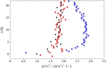
Ratio between the contribution of negatively correlated fluctuation (
 $u^{\prime }w^{\prime }<0$
) and the contribution of positively correlated fluctuation (
 $u^{\prime }w^{\prime }>0$
) contributions for MB
 $_{1}$
(
 $+$
), MB
 $_{2}$
(♢) and CW (○).

Another clear difference between mobile and rigid-bed flow cases, can be seen in the dynamics of inward and outward interactions (quadrants I and III). In order to highlight this point, the absolute value of the ratio between the cumulative contribution of ejection and sweep events (
 $\langle u^{\prime }w^{\prime }\rangle ^{-}$
, quadrants II and IV) and the cumulative contribution of interaction events (
 $\langle u^{\prime }w^{\prime }\rangle ^{+}$
, quadrants I and III) is calculated using the intrinsic averaging process and for
 $H=0$
. The numerator of this ratio contributes to increase the net Reynolds shear stress and the momentum diffusion whereas the denominator contributes to their reduction. The results are shown in figure 6. It can be seen that the ratio is significantly lower for the two mobile-bed cases compared with the clear-water case. One can deduce that the observed increase of turbulence intensities in the upper part of the boundary layer (see figure 1
d,i,e,j) can be attributed to the increase of the contribution of interaction events. As they reduce the mean Reynolds shear stress, these events reduce the turbulent momentum diffusion, whereas they increase the turbulent particles dispersion via the increase of the Reynolds normal stresses. This leads to a reduction of both the von Kármán parameter and the Schmidt number. The modification of the quadrant parameter shown in figure 6 provides a statistical explanation for the reduction of
 $\unicode[STIX]{x1D705}$
and
 $\unicode[STIX]{x1D70E}_{s}$
observed in the presence of sediment transport. This also indicates that the reduction of turbulent momentum mixing is not induced by a damping of turbulent kinetic energy as usually assumed in the literature but rather by an increase of positively correlated
 $u^{\prime }w^{\prime }$
contributions associated with interaction events.
Several mechanisms could explain the modification of the quadrant distribution. In their low-concentration rigid-bed experiment, Kaftori, Hestroni & Banerjee (Reference Kaftori, Hestroni and Banerjee1996) and Niño & Garcia (Reference Niño and Garcia1996) observed a preferential accumulation of particles in strong negatively correlated events as ejections or sweeps events. One can assume that additional inertia associated with the presence of the particles weakens these flow structures (Shao, Wu & Yu Reference Shao, Wu and Yu2012). In Kidanemariam et al. (Reference Kidanemariam, Chan-Braun, Doychev and Uhlmann2013) it was suggested that the preferential direction of inter-particle collisions in the near-bed region could result in a reduction of quadrants II and IV contribution. Unlike the previously mentioned physical and numerical models, the bed is not rigid in the present experiment and it clearly interacts with the large-scale coherent ejection and sweep-type flow structures as visualized in Revil-Baudard et al. (Reference Revil-Baudard, Chauchat, Hurther and Barraud2015). The dynamic bed-disturbance induced by large-scale structures can also explain the relative reduction in ejection and sweep contributions. Even though the present dataset does not permit to discriminate between the different mechanisms, figures 4–6 show that turbulence is modified over a large vertical range, even in low concentration regions (
 $\unicode[STIX]{x1D719}\approx 10^{-3}$
). This observation strongly supports the existence of non-local turbulence effects in the present sediment transport flows. One can conclude that the turbulence is modified either during the production process, i.e. in the near-bed region where the mean velocity shear rate is large, or during the upward diffusion. Two-phase large eddy simulation (LES) approaches currently under development should be an appropriate tool to address these issues.
4 Conclusion
Acoustic high-resolution measurements of velocity and concentration have been performed in two intense mobile-bed flow conditions corresponding to Shields numbers
 $\unicode[STIX]{x1D703}\approx 0.5$
and suspension numbers
 $S\approx 1$
. It is confirmed that the logarithmic formulation of the law of the wall and the Rouse profile are valid under such conditions and that they can be used to predict the mean velocity and concentration profiles in the suspension layer provided that
 $u_{\ast }$
,
 $\unicode[STIX]{x1D705}$
,
 $\unicode[STIX]{x1D70E}_{s}$
,
 $z_{d}$
and the boundary conditions are known.
The origin of the mixing length
 $z_{d}$
is found to be located close to the average position of the fluctuating bed interface, where the local sediment flux is close to its maximum value. In the literature,
 $z_{d}$
is seen as (i) the average level of penetration of large-scale turbulent structures and (ii) the actual level of momentum transfer from the fluid flow to the bed. From these interpretations we conclude that the large-scale turbulent eddies responsible for the momentum diffusion in the logarithmic layer are also responsible for the bed-level fluctuations and part of the momentum transfer to the solid phase.
The comparison between intrinsic and superficial shear stresses reveals the existence of a bed-variability-induced shear stress resulting in an increase of the roughness sublayer thickness. This effect might provide an explanation for the increased flow resistance observed for intense sediment transport in the literature (Wilson Reference Wilson1989; Sumer et al. Reference Sumer, Kozakiewicz, Fredsøe and Deigaard1996; Gao & Abrahams Reference Gao and Abrahams2004; Camenen, Bayram & Larson Reference Camenen, Bayram and Larson2006; Recking et al. Reference Recking, Frey, Paquier, Belleudy and Champagne2008).
The quadrant distribution shows that the additional mobile-bed-induced TKE is associated with an increased contribution of interactions events (i.e. quadrants I and III with
 $u^{\prime }w^{\prime }>0$
). As such interactions events reduce turbulent momentum diffusion and increase particles dispersion, it is consistent with the lower values of the Schmidt number and of the von Kármán parameter observed in the literature over the past decades for intense sediment-laden flows (e.g. Vanoni Reference Vanoni1946; Gaudio et al.
Reference Gaudio, Miglio and Dey2010; Castro-Orgaz et al.
Reference Castro-Orgaz, Giráldez, Mateos and Dey2012).
The measurements reported in this paper present turbulent quantities under intense sediment-laden flows conditions. Such data are crucially needed for the validation of two-phase LES simulations. In turn, high-resolution two-phase flow simulations will help to identify the leading terms of momentum and TKE fluxes and to provide physically-based models for
 $u_{\ast }$
,
 $\unicode[STIX]{x1D705}$
,
 $\unicode[STIX]{x1D70E}_{s}$
, and
 $z_{d}$
under energetic mobile-bed flow conditions.