
 δ
 δ
 δ
 δ



1. Introduction
Shallow water equations were derived (Friedrichs Reference Friedrichs1948) from the continuity and Euler equations under the assumption that the flow is potential and satisfies the long wave approximation (LWA), due to which the characteristic depth
 $H$
of the flow is much smaller than the characteristic length (horizontal size)
 $L$
of the surface waves
 \begin{equation} \varepsilon =H^2/L^2\ll 1. \end{equation}
It follows from this inequality (Stocker Reference Stocker1957) that the spatial derivative of the depth
 $h(x,t)$
of one-dimensional flow satisfies the condition
 \begin{equation} |h_x|\leqslant O(\sqrt {\varepsilon }). \end{equation}
At the same time, the equations of the shallow water theory are widely used for modelling fast wave processes associated with propagation of the hydraulic bores generated by total or partial dam breaks (Stocker Reference Stocker1957; Henderson Reference Henderson1966; Delis & Skeels Reference Delis and Skeels1998; Wang et al. Reference Wang, Ni and He2000; Gottardi & Venutelli Reference Gottardi and Venutelli2003; Borisova & Ostapenko Reference Borisova and Ostapenko2006) or by the impact of large sea tsunami-type waves on a shallow area and an inclined shore (Hibberd & Peregrine Reference Hibberd and Peregrine1979; Yeh et al. Reference Yeh, Liu and Synolakis1996). In this case, the equations are used in the form of a hyperbolic system of conservation laws with convex extension (Friedrichs & Lax Reference Friedrichs and Lax1971), which admits discontinuous solutions with the shocks (Lax Reference Lax1973) used to model the hydraulic bores of real flows. As the width (transverse size) of the shock front is equal to zero, we have a contradiction with the LWA condition (1.2). To resolve this contradiction within the framework of the shallow water theory, we have to assume (Ostapenko Reference Ostapenko2007) that shocks describe the hydraulic bores or jumps whose width
 $l$
is much greater than the characteristic depth of the flow
 $H$
; simultaneously, it is much smaller than the characteristic wave length
 $L$
. Therefore, the following double inequality should be satisfied:
 \begin{equation} H\ll l\ll L. \end{equation}
However, real observations and results of laboratory modelling (Dressler Reference Dressler1954; Chow Reference Chow1959; Brock Reference Brock1969; Hager & Bremen Reference Hager and Bremen1989; Hornung et al. Reference Hornung, Willert and Turner1995; Stansby et al. Reference Stansby, Chegini and Barnes1998) show that the width
 $l$
of the real hydraulic bores is comparable with the characteristic depth
 $H$
of the considered flows, i.e.
 $l=O(H)$
, and does not satisfy the LWA condition (1.3). Nevertheless, a comparison of exact discontinuous solutions of the different shallow water models with the results of laboratory experiments for the dam break problem above a horizontal bottom (Henderson Reference Henderson1966; Stansby et al. Reference Stansby, Chegini and Barnes1998), including the case of a dry bed in the downstream (Ostapenko Reference Ostapenko2007), above a bottom step (Bukreev et al. Reference Bukreev, Gusev and Ostapenko2003), above a shelf-type roughness element of the bottom (Bukreev et al. Reference Bukreev, Gusev and Ostapenko2004b
), above a horizontal bottom in a channel with a bottom step in the downstream water (Gusev et al. Reference Gusev, Ostapenko, Malysheva and Malysheva2008), and also in the problems of the distribution of roll waves on an inclined plane (Richard & Gavrilyuk Reference Richard and Gavrilyuk2012) showed that theoretical predictions agree fairly well with the experimental results in terms of the flow types, velocities of the hydraulic bores and averaged depths of the flow behind their fronts. This means that equations of the shallow water theory ensure effective modelling of hydrodynamic flows whose parameters do not satisfy the formal constraints (1.1), (1.2) applied for deriving these equations.
To explain this paradox of the shallow water theory, the local hydrostatic approximation (LHA) was introduced (Ostapenko Reference Ostapenko2018a
,Reference Ostapenko
b
), which generalises the classical long wave approximation (1.1) and is defined as follows: the plane-parallel fluid flow at the point
 $\boldsymbol{x}=(x,z)$
at the time moment
 $t$
satisfies the local hydrostatic approximation with a positive parameter
 $\delta \ll 1$
when the following inequality is fulfilled:
 \begin{equation} w^2(\boldsymbol{x},t)/c^2(\boldsymbol{x},t)\leqslant \delta , \quad c(\boldsymbol{x},t)=\sqrt {gh(\boldsymbol{x},t)}, \end{equation}
where
 $h$
and
 $w$
are the depth and vertical velocity of the liquid and
 $g$
is the acceleration of gravity. The LHA (1.4) was used to justify the application of the first approximation of shallow water theory (Friedrichs Reference Friedrichs1948; Stocker Reference Stocker1957) in modelling wave flows with the hydraulic bores in one-dimensional (Ostapenko Reference Ostapenko2018a
) and two-dimensional (Ostapenko Reference Ostapenko2018b
) cases.
A modification of the local hydrostatic approximation was proposed (Ostapenko Reference Ostapenko2019), when inequality (1.4) is replaced by the following inequality:
 \begin{equation} w^2(\boldsymbol{x},t)/C^2\leqslant \delta , \quad C=\sqrt {gH}, \end{equation}
where
 $H$
is the characteristic flow depth. The LHA (1.5) was used (Ostapenko Reference Ostapenko2019) to study the possibilities of applying the Green–Naghdi equations (Green et al. Reference Green, Laws and Naghdi1974), obtained in the second approximation of the shallow water theory, to simulate plane-parallel wave flows with the undular hydraulic bores. The local hydrostatic approximation (1.5) has also been applied to describe (Kovyrkina & Ostapenko Reference Kovyrkina and Ostapenko2020) the wave flows arising when a symmetric convex body is lifted from the shallow water and to construct (Ostapenko Reference Ostapenko2021, Reference Ostapenko2025) the
 $\delta$
-asymptotics of two-dimensional steady solutions simulating the energy-conserving fluid outflow from a horizontally aligned rectangular duct (Benjamin Reference Benjamin1968). Moreover, in § 4 of the paper by Ostapenko (Reference Ostapenko2021), a physical justification of the LHA notion is proposed for condition (1.5).
In the present paper, we construct and analyse the LHA asymptotics of liquid flows in the hydraulic jumps and solitary waves. Section 2 examines the various methods for introducing dimensionless variables used in modelling plane-parallel flows of an ideal incompressible fluid, discusses the features of these methods and introduces the appropriate terminology. Section 3 presents the formulation of the problem of liquid flows in the hydraulic jumps and solitary waves within the framework of a plane-parallel steady flow of the ideal incompressible fluid over a horizontal bottom. In § 4, using the LHA (1.5), we construct initial (zero-order)
 $\delta$
-asymptotics of two-dimensional solutions simulating these problems. In § 5, the first-order
 $\delta$
-asymptotics of the liquid depth are obtained for the flows under consideration. In §§ 6 and 7, the first-order
 $\delta$
-asymptotics of the horizontal and vertical fluid velocity are constructed for these flows. In § 8, a concept of combined LHA asymptotics is introduced, in which the asymptotic can depend on two different small parameters,
 $\delta$
and
 $\delta _\alpha =O(\delta )$
, thereby allowing improved agreement with laboratory experiments. In § 9, the modified LHA inequality (1.5) in dimensionless form is used to obtain approximate estimates for the boundaries of the applicability domains of the constructed LHA asymptotics. Section 10 provides a comparison between theory and experiment for the hydraulic bore arising in modelling the dam break problem. In § 11, we discuss whether the constructed first-order LHA asymptotics can be used to model liquid flow in solitary waves. Section 12 presents a comparison between theory and experiment in modelling the solitary waves.
2. Different types of dimensionless variables and the appropriate terminology
In the classical derivation (Friedrichs Reference Friedrichs1948; Stocker Reference Stocker1957) of shallow water equations (Saint–Venant equations) from two-dimensional differential equations of continuity and Euler, taking into account the long wave condition (1.1), the following DV (dimensionless variables) were applied
 \begin{equation} x_*=\frac {x}{L}, \quad z_*=\frac {z}{H}, \quad t_*=\frac {\textit{Ct}}{L}, \quad h_*=\frac {h}{H}, \quad u_*=\frac {u}{C}, \quad p_*=\frac {p}{C^2}, \end{equation}
 \begin{equation} w_*=\frac {Hw}{\textit{LC}}= \frac {\sqrt {\varepsilon }w}{C}, \quad C=\sqrt {gH}, \end{equation}
where
 $x$
and
 $z$
are horizontal and vertical coordinates,
 $t$
is a moment in time,
 $h$
is the liquid depth,
 $u$
and
 $w$
are horizontal and vertical liquid velocities,
 $p=\tilde {p}/\rho$
is the specific pressure in the liquid, where
 $\tilde {p}$
is the actual pressure and
 $\rho$
is the constant density of the fluid. In this case, the Saint–Venant equations are obtained in the first and the Green–Naghdi equations in the second approximation with respect to the LWA parameter
 $\varepsilon$
; from here, these are called the first and the second approximation of the shallow water theory.
Currently, to derive the shallow water equations, another dimensionless variable is also applied, in which the variables (2.1) are used and the dimensionless vertical liquid velocity is given by the formula
 \begin{equation} w_{**}=\frac {Lw}{\textit{HC}}= \frac {w}{\sqrt {\varepsilon }C}= \frac {w_*}{\varepsilon }. \end{equation}
A certain advantage of the DV (2.1), (2.3) is associated (Ostapenko Reference Ostapenko2018b
) with the fact that unlike the DV (2.1), (2.2), they preserve the form of the kinematic condition on the free surface for a moving liquid particle and also explicitly introduce the underlying LWA hydrodynamic hypothesis of the smallness of the vertical acceleration of liquid particles compared with the acceleration of gravity
 $g$
. In addition, the use of the dimensionless variables (2.1), (2.3) allows us to obtain the Saint–Venant equations in the zero and the Green–Naghdi equations in the first approximation with respect to the LWA parameter
 $\varepsilon$
; hence, with such dimensionless variables, these are called the zero and the first approximation of the shallow water theory.
In § 4 of the paper by Ostapenko (Reference Ostapenko2021), it is shown that if the LWA condition (1.1) is satisfied throughout the entire fluid region, then using the dimensionless variables (2.1), (2.3), we can obtain that the LHA condition (1.5) is also satisfied in this region for some parameter
 $\delta =O(\varepsilon )$
. The converse result was also established there: if the LHA condition (1.5) is satisfied throughout the entire flow region, then the LWA condition (1.1) is also satisfied in this region for some parameter
 $\varepsilon =O(\delta )$
. Thus, if the long-wave and local hydrostatic conditions (1.1) and (1.5) hold throughout the entire fluid region, the LWA and LHA concepts are equivalent. At the same time, if the long wave condition (1.1) is not satisfied, the local hydrostatic condition (1.5) can still hold in a subregion of the flow. Therefore, the LHA concept is a natural generalisation of the LWA concept.
When deriving the integral conservation laws for shallow water based on the local hydrostatic condition (1.5), the following dimensionless variables are used (Ostapenko Reference Ostapenko2019, Reference Ostapenko2021):
 \begin{equation} x^*=\frac {\sqrt {\delta }}{H}x, \ \ z^*=\frac {z}{H}, \ \ t^*=\frac {\sqrt {\delta }C}{H}t, \ \ h^*=\frac {h}{H}, \ \ u^*=\frac {u}{C}, \ \ p^*=\frac {p}{C^2}, \ \ w^*=\frac {w}{\sqrt {\delta }C}. \end{equation}
From the long wave condition (1.1), it follows that the characteristic wave length
 $L$
can be represented as
 \begin{equation} L=H/\sqrt {\varepsilon }. \end{equation}
Substituting the value (2.5) in the dimensionless variables (2.1), we obtain
 \begin{equation} x_*=\frac {\sqrt {\varepsilon }}{H}x, \quad z_*=\frac {z}{H}, \quad t_*=\frac {\sqrt {\varepsilon }C}{H}t, \quad h_*=\frac {h}{H}, \quad u_*=\frac {u}{C}, \quad p_*=\frac {p}{C^2}. \end{equation}
The comparison of (2.4) with (2.6) and (2.3) shows that formally, DV (2.4) turns into DV (2.1), (2.3) as a result of replacing the local hydrostatic parameter
 $\delta$
with the long wave parameter
 $\varepsilon$
. In this case, however, dimensionless variables (2.1), (2.3) have physical meaning only when the LWA is performed, while variables (2.4) always remain correct in that part of the fluid flow where the LHA is performed.
From the analogy between the DV (2.1), (2.3) and DV (2.4), it follows that when using dimensionless variables (2.4), the Saint–Venant equations are obtained in the zero and the Green–Naghdi equations in the first approximation with respect to a local hydrostatic parameter
 $\delta$
; as a result, they represent the zero and the first
 $\delta$
-approximation of the shallow water theory. Despite this, in the following sections, we will use the traditional terminology (Friedrichs Reference Friedrichs1948; Green et al. Reference Green, Laws and Naghdi1974), and according to the zero-order and first-order
 $\delta$
-asymptotics of the studied liquid flows, we will classify it as the first and the second approximation of the shallow water theory.
3. Statement of the problem
A plane-parallel steady flow of an ideal incompressible fluid over the horizontal bottom in the domain
 \begin{equation} W=\left \{(x,z): \ -\infty \lt x\lt +\infty , \ 0\leqslant z\leqslant h(x) \right \} \end{equation}
is described by the continuity equation
 \begin{equation} u_x+w_z=0 \end{equation}
and by the steady Euler equations
 \begin{equation} uu_x+wu_z+p_x=0, \quad uw_x+ww_z+p_z+g=0. \end{equation}
From (3.2) and (3.3) follow the divergent equations
 \begin{equation} \big (u^2+p\big )_x+(uw)_z=0, \quad (uw)_x+\big (w^2+p+gz\big )_z=0, \end{equation}
 \begin{equation} (uB)_x+(wB)_z=0, \end{equation}
where
 \begin{equation} B=\frac {u^2+w^2}{2}+gz+p \end{equation}
is the Bernoulli function. Equations (3.4) represent the differential form of the conservation laws for horizontal and vertical momentum. Equation (3.5) is the differential form of the total energy conservation law.
Let us integrate the differential equations (3.2), (3.4a
) and (3.5) with respect to
 $z$
from
 $0$
to
 $h$
and with respect to
 $x$
from
 $x_1$
to
 $x_2$
. Taking into account the kinematic condition
 \begin{equation} w(x,h)=u(x,h)h_x \end{equation}
on the free liquid surface and the no-normal-flow condition
 \begin{equation} w(x,0)=0 \end{equation}
on the bottom, we obtain the integral conservation laws for the mass
 \begin{equation} \left .\left (\int _0^hu\,{\rm d}z\right )\right |_{x_1}^{x_2}=0, \end{equation}
horizontal momentum
 \begin{equation} \left . \left (\int _0^h\big (u^2+ p\big )\,{\rm d}z\right )\right |_{x_1}^{x_2}=0 \end{equation}
and total energy
 \begin{equation} \left . \left (\int _0^hu\left (\frac {u^2+w^2}{2}+gz+ p\right )\,{\rm d}z\right )\right |_{x_1}^{x_2}=0 \end{equation}
of the fluid flow.
Introducing the notation
 \begin{equation} v(x)=\frac {1}{h(x)}\int _0^{h(x)}u(x,z)\,{\rm d}z \end{equation}
for the depth-averaged horizontal velocity of the fluid, one can write the integral equation (3.9) as the mass conservation law for the first approximation of the shallow water theory (Stocker Reference Stocker1957)
 \begin{equation} \left .(hv)\right |_{x_1}^{x_2}=0. \end{equation}
Equation (3.13) implies that
 \begin{equation} q=hv=\textrm {const}, \end{equation}
where
 $q$
is the flow rate of the fluid.
We will explore solutions
 \begin{equation} u(x,z), \quad w(x,z), \quad p(x,z), \quad 0\leqslant z\leqslant h(x), \end{equation}
of (3.2), (3.3), (3.9)–(3.11), satisfying the condition (3.8) and the following boundary conditions at infinity:
 \begin{equation} \lim _{x\rightarrow -\infty }h(x)=h_1, \quad \lim _{x\rightarrow -\infty }u(x,z)=v_1, \quad \lim _{x\rightarrow -\infty }w(x,z)=0, \end{equation}
 \begin{equation} \lim _{x\rightarrow +\infty }h(x)=h_2, \quad \lim _{x\rightarrow +\infty }u(x,z)=v_2, \quad \lim _{x\rightarrow +\infty }w(x,z)=0, \end{equation}
where
 \begin{equation} v_1=q/h_1, \quad v_2=q/h_2. \end{equation}
Assuming that the atmospheric pressure is zero, we obtain that the specific pressure on the free surface of the liquid is
 \begin{equation} p(x,h(x))=0. \end{equation}
Fluid depth profile in a hydraulic jump;
 $(a_1,c_1)$
is the
 $x$
-interval, where the loss of the total energy of the incident flow occurs within the framework of the shallow water theory.

Fluid depth profile in a solitary wave.

Since we will use two-dimensional stationary solutions (3.15) to model the flow in the hydraulic jumps (figure 1) and solitary waves (figure 2) at
 $q\gt 0$
, taking into account (3.17), the limiting values (3.16) of these solutions satisfy the inequalities
 \begin{equation} h_2\geqslant h_1\gt 0 \quad \Rightarrow \quad v_1\geqslant v_2\gt 0. \end{equation}
Conditions
 \begin{equation} h_2\gt h_1\gt 0 \quad \Rightarrow \quad v_1\gt v_2\gt 0 \end{equation}
correspond to flow in the stable hydraulic jump and conditions
 \begin{equation} h_2=h_1\gt 0 \quad \Rightarrow \quad v_1=v_2\gt 0 \end{equation}
correspond to flow in the solitary wave.
For finite-amplitude hydraulic jumps and solitary waves, the LWA condition (1.2) is not satisfied throughout the flow region; consequently, such flows cannot be modelled using the LWA approach (1.1). Therefore, we will construct asymptotics of liquid flows in the hydraulic jumps and solitary waves based on the LHA method (1.5).
4. Initial (zero-order)
 $\delta$
-asymptotics of two-dimensional solutions

Taking into account the boundary conditions (3.16), there exists functions
 $a(\delta )$
and
 $b(\delta )\geqslant a(\delta )$
such that the LHA inequality (1.5) is satisfied at all points of the domain
 \begin{equation} V(\delta )=\left \{(x,z)\in W: \ x\leqslant a(\delta ), \ x\geqslant b(\delta ) \right \} \!. \end{equation}
We will assume that in the domain (4.1), the liquid flow (3.15) is potential
 \begin{equation} u_z-w_x=0. \end{equation}
Since in the case of the turbulent hydraulic bores, small-scale vortices are formed behind their fronts, leading to a violation of the flow potentiality (4.2), we restrict our attention to hydraulic jumps with a continuous surface flow, excluding turbulent jumps from the present study.
Note that a specific value of parameter
 $\delta$
included in the LHA inequality (1.5) determines the accuracy with which
 $\delta$
-asymptotics approximate two-dimensional flow (3.15) in the domain (4.1): with an increase in
 $\delta$
, this accuracy decreases and with a decrease in
 $\delta$
, it increases. If the LHA condition (1.5) is not satisfied throughout the flow region (3.1), i.e.
 $V(\delta )\subset W$
, then an increase in parameter
 $\delta$
leads to an expansion of domain
 $V(\delta )$
and a decrease in parameter
 $\delta$
leads to a narrowing of domain
 $V(\delta )$
. If in the two-dimensional flow (3.15) the vertical velocity
 $w(x,z)$
is separated from zero
 \begin{equation} |w(x,z)|\geqslant w_m\gt 0, \quad (x,z)\in W, \end{equation}
then at
 $\delta \rightarrow 0$
, the domain
 $V(\delta )$
degenerates into an empty set.
We will construct the
 $\delta$
-asymptotics of two-dimensional solution (3.15) using integral conservation laws (3.9)–(3.11) defined on intervals
 \begin{equation} [x_1,x_2]: \ (x_1,0),\ (x_2,0)\in V(\delta ). \end{equation}
Equations (3.2), (3.3a ), (3.9), (3.10), (3.12) and (3.14) being written in the dimensionless variables (2.4) remain unchanged, whereas (3.3b ), (3.11) and (4.2) take the form
 \begin{equation} \delta (uw_x+ww_z)+p_z+1=0, \end{equation}
 \begin{equation} \left . \left (\int _0^hu\left (\frac {u^2+\delta w^2}{2}+z+ p\right ){\rm d}z\right )\right |_{x_1}^{x_2}=0, \end{equation}
 \begin{equation} u_z-\delta w_x=0. \end{equation}
Hereinafter, the asterisk at the dimensionless variables is omitted for brevity.
Let us transform the integrals included into momentum conservation law (3.10). Introducing the notation
 \begin{equation} \widetilde {u}=u-v \quad \Leftrightarrow \quad u=v+\widetilde {u}, \end{equation}
and taking into account that
 \begin{equation} \int _0^h\widetilde {u}\,{\rm d}z=\int _0^hu\,{\rm d}z-hv=0, \end{equation}
we obtain
 \begin{equation} \int _0^hu^2\,{\rm d}z= hv^2+\int _0^h\widetilde {u}^2\,{\rm d}z. \end{equation}
Since the fluid velocity function
 $u(x,z)$
in the domain (4.1) is continuous, there is a continuous function
 $z_c(x)\in (0,h(x))$
such that
 \begin{equation} \int _0^{h(x)}u(x,z)\,{\rm d}z=u(x,z_c(x))h(x) \ \Rightarrow \ v(x)=u(x,z_c(x)). \end{equation}
Equation (4.8) with (4.11) and (4.7) in mind can be represented as
 \begin{equation} \widetilde {u}=u-v=\int _{z_c}^zu_z\,{\rm d}z =\delta \int _{z_c}^zw_x\,{\rm d}z, \end{equation}
whence it follows that
 \begin{equation} u=v+\delta \int _{z_c}^zw_x\,{\rm d}z. \end{equation}
Equation (4.12) implies that
 \begin{equation} \int _0^h\widetilde {u}^2\,{\rm d}z=\delta ^2\int _0^h\left (\int _{z_c}^z w_x\,{\rm d}z\right )^2\,{\rm d}z= O(\delta ^2). \end{equation}
As a result, from (4.10), with allowance for (4.14), we have
 \begin{equation} \int _0^hu^2\,{\rm d}z= hv^2+O(\delta ^2). \end{equation}
Integrating the Euler equation (4.5) twice along the vertical coordinate, first from
 $z$
to
 $h$
with
 $z\in [0,h)$
and then from
 $0$
to
 $h$
, and using (3.18), we have
 \begin{equation} \int _0^hp\,{\rm d}z=h^2/2+\delta G, \end{equation}
where
 \begin{equation} G=\int _0^h\left (\int _z^h(uw_x+ww_z)\,{\rm d}z\right )\,{\rm d}z. \end{equation}
From the momentum conservation law (3.10), taking into account condition (4.4) and (4.16), (4.17), with accuracy
 $O(\delta )$
, we obtain
 \begin{equation} \big (hv^2+h^2/2\big ) \big |_{x_1}^{x_2}=0. \end{equation}
Transforming the integrals included in the energy conservation law (4.6), with allowance for (4.8), (4.9), (4.12) and (4.16), we have
 \begin{equation} \int _0^hu^3\,{\rm d}z=hv^3+3v\int _0^h\widetilde {u}^2\,{\rm d}z+\int _0^h\widetilde {u}^3\,{\rm d}z=hv^3+O(\delta ^2), \end{equation}
 \begin{equation} \int _0^huz\,{\rm d}z=\frac {vh^2}{2}+\int _0^h\widetilde {u}z\,{\rm d}z=\frac {vh^2}{2}+O(\delta ), \end{equation}
 \begin{equation} \int _0^hup\,{\rm d}z=v\int _0^hp\,{\rm d}z+\int _0^h\widetilde {u}p\,{\rm d}z=\frac {vh^2}{2}+O(\delta ). \end{equation}
As a result, from integral conservation law (4.6), under condition (4.4) and (3.14), with accuracy
 $O(\delta )$
, we obtain
 \begin{equation} \big (hv^3/2+vh^2\big )\big |_{x_1}^{x_2}= q \big(v^2/2+h\big )\big |_{x_1}^{x_2}=0. \end{equation}
Since in the considered problems (3.15)–(3.19) the liquid flow rate
 $q\gt 0$
, (4.22) can be rewritten as
 \begin{equation} \big (v^2/2+h\big )\big|_{x_1}^{x_2}=0. \end{equation}
Equations (4.18) and (4.23) represent an analogue of the Rankine–Hugoniot shock wave conditions (Lax Reference Lax1973) for the momentum and energy conservation laws of the stationary Saint–Venant equations corresponding to the first approximation of the shallow water theory (Stocker Reference Stocker1957). When one of two conditions
 \begin{equation} x_1\lt x_2\leqslant a(\delta ), \quad x_2\gt x_1\geqslant b(\delta ) \end{equation}
is met, i.e. if integration segment
 $[x_1,x_2]$
is entirely located in one of the subdomains of doubly connected domain (4.1), then the liquid flow on this segment is smooth and potential, due to which the momentum (4.18) and energy (4.23) conservation laws are simultaneously satisfied on segment
 $[x_1,x_2]$
. Since (4.18) and (4.23) are compatible only under condition
 \begin{equation} h(x_1)=h(x_2) \quad \Rightarrow \quad v(x_1)=v(x_2), \end{equation}
see, for example, Ostapenko (Reference Ostapenko2014), then taking into account (4.13) and boundary conditions (3.16), with accuracy
 $O(\delta )$
, we obtain
 \begin{equation} h(x)=\left \{ \begin{array}{ll} h_1, & x\leqslant a(\delta ), \\[3pt] h_2, & x\geqslant b(\delta ), \end{array} \right . \quad u(x,z)=v(x)=\left \{ \begin{array}{ll} v_1, & x\leqslant a(\delta ), \\[3pt] v_2, & x\geqslant b(\delta ). \end{array} \right . \end{equation}
Integrating the continuity equation (3.2) along the vertical coordinate from
 $0$
to
 $z$
, with the no-normal-flow condition (3.8) and (4.13) in mind, we have
 \begin{equation} w=\int _0^zw_z\,{\rm d}z=-\int _0^zu_x\,{\rm d}z= -zv_x-\delta J, \end{equation}
where
 \begin{equation} J=\int _0^z\left (\frac {\partial }{\partial x}\int _{z_c}^z w_x\,{\rm d}z\right )\,{\rm d}z. \end{equation}
From (4.27) and (4.26b
), with accuracy
 $O(\delta )$
, we obtain
 \begin{equation} w(x,z)=0, \quad (x,z)\in V(\delta ). \end{equation}
Let us assume that conditions (3.20) corresponding to the hydraulic jump are satisfied simultaneously with inequalities
 \begin{equation} x_1\leqslant a(\delta )\lt b(\delta )\leqslant x_2, \end{equation}
from which it follows that integration segment
 $[x_1,x_2]$
contains finite transition interval
 $(a(\delta ),b(\delta ))$
, on where the LHA conditions (1.5) are not satisfied. In this case, the energy conservation law (4.23) is not satisfied and, within the framework of theory of the hyperbolic system of conservation laws with convex extension (Friedrichs & Lax Reference Friedrichs and Lax1971), the conservation law (4.23) is transformed into the energy (entropy) inequality
 \begin{equation} \big (v^2+2h\big )\big|_{x_1}^{x_2}\lt 0, \end{equation}
intended for the selection of the stable hydraulic jumps, at which the energy of the passing fluid flow is lost in the sense that some part of it is converted into the energy of small-scale fluid oscillations, not taken into account in the Saint–Venant equations.
As a result, from the momentum conservation law (4.18), with allowance for (3.17), we obtain
 \begin{equation} \left . \left (\frac {q^2}{h}+\frac {h^2}{2}\right )\right |_{x_1}^{x_2}=0 \quad \Leftrightarrow \quad \frac {q^2}{h_2}+\frac {h_2^2}{2}= \frac {q^2}{h_1}+\frac {h_1^2}{2}. \end{equation}
The second equation (4.32) can be rewritten as
 \begin{equation} q^2\left (\frac {1}{h_1}-\frac {1}{h_2}\right )= \frac {q^2(h_2-h_1)}{h_1h_2}= \frac {h_2^2-h_1^2}{2}. \end{equation}
From here, taking into account (3.20), we have
 \begin{equation} q^2=h_1h_2\overline {h}, \end{equation}
where
 \begin{equation} h_2\gt \overline {h}=(h_1+h_2)/2\gt h_1. \end{equation}
As noted by Rouse & Ince (Reference Rouse and Ince1963), the correct relationship (4.34) for the flow parameters at a hydraulic jump was first obtained by Bresse (Reference Bresse1860).
From (4.34) under (4.35), it follows that flow
 $(h_1,v_1)$
is supercritical
 \begin{equation} v_1^2=q^2/h_1^2=h_2\overline {h}/h_1\gt c_1^2=h_1 \end{equation}
and flow
 $(h_2,v_2)$
is subcritical
 \begin{equation} v_2^2=q^2/h_2^2=h_1\overline {h}/h_2\lt c_2^2=h_2, \end{equation}
where
 $c_1=\sqrt {h_1}$
and
 $c_2=\sqrt {h_2}$
are the propagation velocities of small disturbances in the shallow water. From the supercriticality of the incoming flow
 $(h_1,v_1)$
, it follows that the characteristics of this flow propagate with positive velocities
 $v_1\pm c_1\gt 0$
. Physically, this means that within the framework of the Saint–Venant equations of the first approximation of the shallow water theory, the outgoing flow
 $(h_2,v_2)$
has no effect on the incoming flow
 $(h_1,v_1)$
.
Let us introduce an abbreviated notation
 \begin{equation} [f]=\left . f\right |_{x_1}^{x_2}=f(x_2)-f(x_1), \end{equation}
with which we can rewrite the energy inequality (4.31) in the form
 \begin{equation} [v^2+2h]=q^2\big [h^{-2}\big ]+2[h]= 2[h]-q^2 \big[h^2\big]/(h_1h_2)^2= 2[h]\big (1-q^2\overline {h}/(h_1h_2)^2\big )\lt 0, \end{equation}
where
 $[h]=h_2-h_1$
. Substituting (4.34), we obtain
 \begin{equation} [v^2+2h]= 2[h]\big (1-\overline {h}^2/(h_1h_2)\big )= -[h]^3/(2h_1h_2)\lt 0. \end{equation}
This inequality is true when the condition (4.35) is met. This means that the hydraulic jumps satisfying (3.20) are energetically stable.
If the depth
 $h_1$
is given, from (4.34), it follows that the depth
 $h_2$
is the positive root of the quadratic equation
 \begin{equation} h_1h^2+h_1^2h-2q^2=0 \end{equation}
and is calculated by the formula
 \begin{equation} h_2=\frac {\sqrt {h_1^4+8h_1q^2}-h_1^2}{2h_1} \quad \Rightarrow \quad v_2=\frac {q}{h_2}. \end{equation}
Equations (4.42) define a two-parameter family of solutions (4.26), where depth
 $h_1$
and flow rate
 $q$
are given parameters that satisfy conditions (4.36) and (4.37).
The family of piecewise constant solutions (4.26), (4.29), (4.42) constructed in domain (4.1), where
 $a(\delta )\lt b(\delta )$
, represents the zero-order
 $\delta$
-asymptotics of two-dimensional solution (3.15) simulating the liquid flows in the steady hydraulic jumps. These asymptotics correspond to a two-parameter family
 \begin{equation} h(x)=\left \{ \begin{array}{ll} h_1, & x\leqslant c(\delta ), \\[3pt] h_2, & x\gt c(\delta ), \end{array} \right . \quad v(x)=\left \{ \begin{array}{ll} v_1, & x\leqslant c(\delta ), \\[3pt] v_2, & x\gt c(\delta ), \end{array} \right . \end{equation}
where
 $c(\delta )\in (a(\delta ),b(\delta ))$
, of stable discontinuous piecewise constant solutions of the Saint–Venant equations obtained using the Rankine–Hugoniot condition
 \begin{equation} \big (hv^2+h^2/2\big ) \big |_{c(\delta )}^{c(\delta )+0}=0 \end{equation}
for the steady momentum conservation law. Since
 $\delta$
-asymptotics (4.26) are not defined on the interval
 $(a(\delta ),b(\delta ))$
, the discontinuous solution (4.43) approximates the two-dimensional flow (3.15) in the hydraulic jumps only outside the interval
 $(a(\delta ),b(\delta ))$
. Despite this, the above-mentioned result can be considered as an independent, additional to that of Ostapenko (Reference Ostapenko2018a
), justification for the applicability of the first approximation of the shallow water theory for modelling wave flows with the hydraulic bores and jumps.
Note that introducing the fluid viscosity into the momentum conservation law (4.18) allows (Razis et al. Reference Razis, Kanellopoulos and Weele2021) to construct smooth solutions of Saint–Venant equations, which model the steady hydraulic jump in an inclined channel.
If two-dimensional solution (3.15) models the solitary wave for which the conditions (3.21) are fulfilled, (4.26) are simplified and can be written as
 \begin{equation} h(x)=h_1, \quad (x,0)\in V(\delta ); \quad u(x,z)=v(x)=v_1, \quad (x,0)\in V(\delta ). \end{equation}
This means that in the initial (zero-order)
 $\delta$
-asymptotics, a solitary wave is not possible.
5. The first-order
$\delta$
-asymptotics for the liquid depth

To construct the first-order
 $\delta$
-asymptotics for the liquid depth, we will use two-dimensional momentum conservation laws (3.10), defined on the intervals
 $[x_1,x_2]$
, with boundaries satisfying condition (4.24a
).
Let us consider a streamline
 \begin{equation} x=x_s(\tau ), \quad z=z_s(\tau ) \end{equation}
of the two-dimensional steady flow (3.16). We will assume that this streamline is parametrised in such a way that the fluid velocities are given by the formulae
 \begin{equation} u(x_s(\tau ),z_s(\tau ))=\frac {{\rm d}x_s(\tau )}{{\rm d}\tau },\quad w(x_s(\tau ),z_s(\tau ))=\frac {{\rm d}z_s(\tau )}{{\rm d}\tau }. \end{equation}
In this case, the derivative of an arbitrary function
 $f(x,z)$
along a streamline (5.1) is written as follows:
 \begin{equation} \dot {f}\equiv \frac {{\rm d}f(x_s,z_s)}{{\rm d}\tau }= u(x_s,z_s)f_x(x_s,z_s)+w(x_s,z_s)f_z(x_s,z_s). \end{equation}
Omitting the arguments for simplicity, we have
 \begin{equation} \dot {f}= uf_x+wf_z. \end{equation}
In particular, for the derivative of depth and vertical acceleration of the fluid, we obtain
 \begin{equation} \dot {h}=uh_x, \quad \dot {w}=uw_x+ww_z. \end{equation}
Differentiating equality (3.14), with allowance for formulae (4.13) and (5.10), we have
 \begin{align} hv_x+vh_x=0 \quad \Rightarrow \quad v_x=-\frac {vh_x}{h}= -\frac {\dot {h}}{h}+O(\delta ). \end{align}
Substituting (5.6b ) in (4.27), we obtain (Boussinesq Reference Boussinesq1877)
 \begin{equation} w=z\dot {h}/h+O(\delta ). \end{equation}
Differentiating (5.7) along the streamline, with accuracy
 $O(\delta )$
, we have
 \begin{equation} \dot {w}=\frac {\rm d}{{\rm d}t}\left ( \frac {z\dot {h}}{h}\right )=\frac {1}{h^2} \left (h\frac {{\rm d}(z\dot {h})}{{\rm d}t}- z(\dot {h})^2\right )\!. \end{equation}
Since, together with (5.7), we obtain
 \begin{equation} \frac {{\rm d}(z\dot {h})}{{\rm d}t}=w\dot {h}+z\ddot {h}=\frac {z(\dot {h})^2}{h}+z\ddot {h} +O(\delta ), \end{equation}
substituting representation (5.9) in (5.8), with accuracy
 $O(\delta )$
, we have
 \begin{equation} \dot {w}=\frac {1}{h^2} \left (h\left (\frac {z(\dot {h})^2}{h}+ z\ddot {h}\right )-z(\dot {h})^2\right )= \frac {z\ddot {h}}{h}. \end{equation}
From (4.17) under equalities (5.5) and (5.10), with accuracy
 $O(\delta )$
, we obtain
 \begin{equation} G=\frac {\ddot {h}}{h}\int _0^h\left (\int _z^hz\,{\rm d}z\right )\,{\rm d}z=\frac {h^2\ddot {h}}{3}. \end{equation}
As a result, from two-dimensional momentum conservation law (3.10), with allowance for (3.14), (4.15)–(4.17) and (5.11), with accuracy
 $O(\delta ^2)$
, we obtain the momentum conservation law
 \begin{equation} \left .\left (q^2/h+h^2/2+\delta h^2\ddot {h}/3\right )\right |_{x_1}^{x_2}=0 \end{equation}
for the steady Green–Naghdi equations (Green et al. Reference Green, Laws and Naghdi1974) of the second approximation of shallow water theory. Taking into account the basic papers (Boussinesq Reference Boussinesq1877; Serre Reference Serre1953), (5.12) and its modifications are also called the fully nonlinear Boussinesq equations (Gobbi et al. Reference Gobbi, Kirby and Wei2000; Madsen et al. Reference Madsen, Bingham and Liu2002), as well as the Serre–Green–Naghdi equations (Chhay et al. Reference Chhay, Dutykh and Clamond2016; Cocquet et al. Reference Cocquet, Mihami, Moguen and Roeber2024).
Let us construct in the domain
 $x\leqslant a(\delta )$
a strictly monotonically increasing solution
 \begin{equation} h=h(x)=h(x_2), \quad x=x_2\leqslant a(\delta ) \end{equation}
of (5.12), that with the boundary conditions (3.16a ), satisfies the following conditions:
 \begin{equation} \lim _{x\rightarrow -\infty }h'(x)= \lim _{x\rightarrow -\infty }h''(x)=0 \quad \Rightarrow \quad \lim _{x\rightarrow -\infty }\ddot {h}(x)=0, \end{equation}
where
 \begin{equation} \ddot {h}=u(\dot {h})_x=u(uh_x)_x= \frac {q^2}{h}\left (h_x/h\right )_x=\frac {q^2}{h^3} \big (hh''-(h')^2\big ), \quad h'=h_x\gt 0. \end{equation}
Passing in (5.12) to the limit at
 $x_1\rightarrow -\infty$
, using the designation (5.13) and boundary conditions (3.16a
), (5.14), we have
 \begin{equation} q^2/h+h^2/2+\delta h^2\ddot {h}/3= q^2/h_1+h_1^2/2. \end{equation}
With (5.15) in mind, (5.16) can be represented as
 \begin{equation} h''-\frac {(h')^2}{h}=F(h), \quad F(h)=\frac {3(h-h_1)\left (2q^2-h_1h(h+h_1) \right )}{2\delta q^2h_1h}. \end{equation}
The condition
 $h'\gt 0$
allows us to apply the standard substitution
 \begin{equation} \eta (h)=(h')^2 \quad \Rightarrow \quad (\eta (h))'=\eta 'h'=2h'h'' \quad \Rightarrow \quad h''=\eta '/2, \end{equation}
and so (5.17) can be rewritten as
 \begin{equation} \eta '-2\eta /h=2F(h). \end{equation}
Integrating (5.19) with boundary condition
 \begin{equation} \eta (h_1)=\eta \left (\lim _{x\rightarrow - \infty }h(x)\right )=\left (\lim _{x\rightarrow - \infty }h'(x)\right )^2=0, \end{equation}
we obtain
 \begin{equation} \eta =(h')^2=\frac {3(h-h_1)^2(q^2-h_1^2h)} {\delta q^2h_1^2}. \end{equation}
If inequalities (4.32) are satisfied, it follows that the flow
 $(h_1,v_1)$
is supercritical and (5.21) has real solutions at depths
 \begin{equation} h=h(x)\in (h_1,\hat {h}], \quad \hat {h}=v_1^2=q^2/h_1^2, \end{equation}
when the right-hand side of this equation is non-negative. Since from (5.22) under inequalities (4.32) we have
 \begin{equation} \hat {v}=q/\hat {h}=h_1^2/q= h_1/v_1\lt v_1=\sqrt {\hat {h}}, \end{equation}
flow
 $(\hat {h},\hat {v})$
at the right boundary of the interval
 $(h_1,\hat {h}]$
is subcritical. Under condition (5.22) from (5.21), in accordance with
 $h'\gt 0$
at
 $h\in (h_1,\hat {h})$
, we obtain
 \begin{equation} h'=\frac {h-h_1}{qh_1} \sqrt {\frac {3(q^2-h_1^2h)}{\delta }}. \end{equation}
By integrating (5.24), we have
 \begin{equation} h(x)=v_1^2-\big (v_1^2-h_1\big )\tanh ^2\left ( \sqrt {\frac {3(v_1^2-h_1)}{\delta }} \ \frac {x-x_0}{q} \right )\!, \end{equation}
where
 $\tanh (x)$
is the hyperbolic tangent function and
 $x_0$
is the constant of integration. Applying (5.22), solution (5.25) is determined for
 $x\leqslant x_0$
. Note that function (5.25) and its various modifications are widely used to model the solitary wave profile; refer to seminal papers (Rayleigh Reference Rayleigh1876; Korteweg & de Vries Reference Korteweg and de Vries1895) and review papers (Yeh et al. Reference Yeh, Liu and Synolakis1996; Jager Reference Jager2011). In our case, (5.25) under condition (5.22) represents the first-order
 $\delta$
-asymptotics for the liquid depth on the left side of both the hydraulic jump and the solitary wave. The parameter
 $x_0$
, in the general case, should be selected by agreement with laboratory experiments, as done by Ostapenko (Reference Ostapenko2021), when constructing asymptotics for the fluid outflow from a rectangular duct (Benjamin Reference Benjamin1968).
Now, we will consider the momentum conservation laws (3.10), defined on intervals
 $[x_1,x_2]$
with boundaries satisfying condition (4.24b
), that, as in the previous case, leads to the Green–Naghdi equation (5.12). Let us try to construct on a semi-infinite interval
 \begin{equation} [\tilde {x},+\infty )\subset [b(\delta ),+\infty ), \end{equation}
a strictly monotonically increasing or decreasing solution
 \begin{equation} h=h(x)=h(x_1), \quad x=x_1\geqslant \tilde {x} \end{equation}
of (5.12) that, with boundary conditions (3.16b ) corresponding to the hydraulic jump under inequalities (3.20), satisfies the following conditions:
 \begin{equation} \lim _{x\rightarrow +\infty }h'(x)= \lim _{x\rightarrow +\infty }h''(x)=0 \quad \Rightarrow \quad \lim _{x\rightarrow +\infty }\ddot {h}(x)=0. \end{equation}
Passing in (5.12) to the limit at
 $x_2\rightarrow +\infty$
, using the designation (5.27) and boundary conditions (3.16b
), (5.28), we again, as in the previous case, obtain the equation
 \begin{equation} \eta =(h')^2=\frac {3(h-h_2)^2(q^2-h_2^2h)} {\delta q^2h_2^2}. \end{equation}
Since the flow
 $(h_2,v_2)$
is subcritical (4.36), then at depths
 \begin{equation} h=h(x)\in (\check {h},+\infty ], \quad \check {h}=v_2^2=q^2/h_2^2\lt h_2, \end{equation}
the right-hand side of (5.29) is negative and it has no real solutions. This means that there is no interval (5.26) where (5.12) has a strictly monotone solution (5.27) satisfying the boundary conditions (3.16b
) and (5.28). It follows that in the domain
 $x\geqslant b(\delta )$
behind the hydraulic jump, two-dimensional flow (3.15) does not allow the regular first-order
 $\delta$
-asymptotics for the liquid depth and therefore the Green–Naghdi equations are difficult to use for correct modelling of wave flows with the hydraulic bores and jumps. This is confirmed by numerical calculations (El et al. Reference El, Grimshaw and Smyth2006; Metayer et al. Reference Metayer, Gavrilyuk and Hank2010) using the Green–Naghdi equations for the dam break problem. These calculations failed to effectively reproduce the sequence of damped surface waves behind the undular bore because the amplitude and the length of numerical waves differ significantly from those observed in the laboratory experiments (Henderson Reference Henderson1966; Bukreev et al. Reference Bukreev, Gusev and Ostapenko2003).
In the case of the solitary wave, for which
 $h_2=h_1$
, the strictly monotonically decreasing solution
 \begin{equation} h=h(x)=h(x_1), \quad x=x_1\geqslant b(\delta ) \end{equation}
of (5.12) is defined under condition (5.22) and is given by
 \begin{equation} h(x)=v_1^2-\big (v_1^2-h_1\big ) \tanh ^2\left ( \sqrt {\frac {3(v_1^2-h_1)}{\delta }} \ \frac {x-\tilde {x}_0}{q} \right )\!, \quad x\geqslant \tilde {x}_0, \end{equation}
where
 $\tilde {x}_0$
is the constant of integration. Note that solution (5.32) is obtained by integrating the equation
 \begin{equation} h'=-\frac {h-h_1}{qh_1} \sqrt {\frac {3(q^2-h_1^2h)}{\delta }} \end{equation}
in the domain
 $x\geqslant b(\delta )$
.
Since (5.25) and (5.32) are similar, then further, when constructing the first-order
 $\delta$
-asymptotics for the horizontal and vertical liquid velocities, we will obtain them using (5.25), which defines such asymptotics for both hydraulic jump and solitary wave. Taking this into account, we will further use
 $H=h_1$
as the characteristic liquid depth included in the LHA inequality (1.5); as a result, from (2.4), it follows that the dimensionless value of the depth
 $h_1=1$
. This allows us to rewrite (5.24) and (5.25) in the following simpler form:
 \begin{equation} h'=\frac {h-1}{q} \sqrt {\frac {3(q^2-h)}{\delta }}, \end{equation}
 \begin{equation} h(x)=q^2-\big (q^2-1\big )\tanh ^2\left ( \sqrt {\frac {3(q^2-1)}{\delta }} \ \frac {x-x_0}{q} \right )\!, \quad x\leqslant x_0. \end{equation}
The applicability condition (5.22) of these formulae takes the form
 \begin{equation} h=h(x)\in (1,q^2]. \end{equation}
Figures 3 and 4 show graphs of the functions
 $h(x)$
, given by (5.35), where
 $x_0=0$
. In figure 3, the graphs of this function is shown at a constant value of the LHA parameter
 $\delta =0.05$
and four different values of the flow liquid rate
 $q$
. In figure 4, these graphs are shown at a constant value of
 $q=1.3$
and four different values of
 $\delta$
.
Graphs of the liquid depth
 $h(x)$
given by (5.35) at
 $x_0=0$
and
 $\delta =0.05$
with four different values of the flow rate
 $q=1.1$
(line 1),
 $q=1.2$
(line 2),
 $q=1.3$
(line 3) and
 $q=1.4$
(line 4). The dotted parts of graphs correspond to those areas of fluid flow where the LHA condition (9.1) is not met.

Graphs of the liquid depth
 $h(x)$
given by (5.35) at
 $x_0=0$
and
 $q = 1.3$
with four different values of the LHA parameter
 $\delta =0.025$
(line 1),
 $\delta =0.05$
(line 2),
 $\delta =0.075$
(line 3) and
 $\delta =0.1$
(line 4). The dotted parts of graphs correspond to those areas of fluid flow where the LHA condition (9.1) is not met.

6. First-order
$\delta$
-asymptotics for horizontal fluid velocity

From the mass conservation law (3.14), we obtain that at
 $x\leqslant a(\delta )$
, the first-order
 $\delta$
-asymptotics for the depth-averaged horizontal fluid velocity (3.12) is determined by
 \begin{equation} v(x)=q/h(x), \end{equation}
where the liquid depth
 $h(x)$
is given by (5.35). The graphs of function (6.1) at
 $x_0=0$
, and different values of parameters
 $q$
and
 $\delta$
are easily obtained from the liquid depth graphs shown in figures 3 and 4.
Let us construct at
 $x\leqslant a(\delta )$
the first-order
 $\delta$
-asymptotics for the horizontal fluid velocity
 $u(x,z)$
. To do this, we substitute (5.7) in (4.13), represented as
 \begin{equation} w=zuh'/h+O(\delta )=-zq\theta '+ O(\delta ), \end{equation}
where
 \begin{equation} \theta =1/h \quad \Rightarrow \quad \theta '=(1/h)'=-h'/h^2. \end{equation}
As a result, with accuracy
 $O(\delta ^2)$
, we obtain
 \begin{equation} u=v-\frac {1}{2}\delta q\theta ''\big (z^2-z_c^2\big ), \end{equation}
where
 \begin{equation} \theta ''=\left (\frac {1}{h}\right )''= \frac {2(h')^2-hh''}{h^3}, \end{equation}
derivative
 $h'$
is given by (5.34) and derivative
 \begin{equation} h''=\frac {{\rm d}h'}{{\rm d}h}h'= \frac {3}{\delta q^2}(h-1)(q^2-h-1/2). \end{equation}
To determine the function
 $z_c(x)$
, let us substitute in (3.12) the value of horizontal fluid velocity given by (6.4). As a result, with accuracy
 $O(\delta ^2)$
, we have
 \begin{equation} v=\frac {1}{h}\int _0^hu\,{\rm d}z=v-\frac {1}{2}\delta q\theta ''\left . \left (\frac {z^3}{3}- z_c^2z\right )\right |_0^h \! . \end{equation}
Hence, it follows that
 \begin{equation} \frac {h^3}{3}-z_c^2h=0 \quad \Leftrightarrow \quad z_c(x)=\frac {h(x)}{\sqrt {3}}. \end{equation}
Thus, with (6.4), we obtain that the first-order
 $\delta$
-asymptotics for the horizontal fluid velocity has the form
 \begin{equation} u=v+\frac {1}{2}\delta q\theta ''\left (\frac {h^2}{3}-z^2\right )\!, \end{equation}
where the depth-averaged velocity
 $v=v(h,q)$
is given by (6.1), the function
 $\theta ''=\theta ''(h,q,\delta )$
is defined by (6.5), (5.34), (6.6) and the depth
 $h=h(x,q,\delta )$
is given by (5.35). From (6.9), it follows that at line
 \begin{equation} z(x)=z_c(x)=h(x)/\sqrt {3} ,\end{equation}
the horizontal velocity
 $u(x,z)$
with accuracy
 $O(\delta ^2)$
coincides with the depth-averaged velocity
 $v(x)$
, i.e.
 \begin{equation} u(x,z_c(x))=v(x)+O(\delta ^2). \end{equation}
The behaviour of function (6.9) significantly depends on the sign of derivative (6.5), which, under (5.34) and (6.6), can be written in the form
 \begin{equation} \theta ''=\frac {3(q-h)\varphi (q,h)}{2\delta q^2h^3}, \end{equation}
where
 \begin{equation} \varphi (q,h)=2h^2-(2q^2+5)h+4q^2. \end{equation}
Since
 \begin{equation} 2h^2-(2q^2+5)h+4q^2=0 \end{equation}
has real roots
 \begin{equation} h_\pm =\frac {1}{4}\left (2q^2+ 5\pm \sqrt {4q^4+12q^2+25} \right ) \end{equation}
such that
 $h_+\gt q^2$
and
 $h_-\lt 1$
, then (6.13) is negative and (6.12) is positive on the applicability interval (5.36). It follows that (6.9) is strictly monotonically decreasing in the z-coordinate in the entire domain
 $x\leqslant a(\delta )$
of constructing the first-order
 $\delta$
-asymptotics, due to which in this domain, the horizontal fluid velocity at the bottom is greater than at the flow surface
 \begin{equation} u(x,0)\gt v(x)\gt u(x,h(x)). \end{equation}
We give the physical justification for this result at the end of § 7.
Graphs of the horizontal fluid velocity
 $u=u(z,h)$
given by (6.9) as a function of the vertical coordinate
 $z$
(thick lines) compared with the depth-averaged velocity
 $v$
(thin lines) at
 $x_0=0$
,
 $\delta =0.05$
,
 $q = 1.3$
, and four different values of the liquid depth
 $h=1.1$
(lines 1),
 $h=1.2$
(lines 2),
 $h=1.3$
(lines 3) and
 $h=1.6$
(lines 4). Lines 3 are dotted because at
 $h=1.3$
, the flow does not satisfy the LHA condition (9.1).

Figure 5 shows the horizontal fluid velocity
 $u=u(z,h)$
given by (6.9) as a function of vertical coordinate
 $z\in (0,h]$
compared with the depth-averaged velocity
 $v=q/h$
at
 $x_0=0$
,
 $\delta =0.05$
,
 $q = 1.3$
and four different values of the flow depth
 $h$
.
7. First-order
$\delta$
-asymptotics for vertical fluid velocity

Let us substitute in the integral formula (4.28) the derivative
 \begin{equation} w_x=-zq\theta ''+ O(\delta ), \end{equation}
obtained as a result of differentiation of relation (6.2). As a result, under (6.8), with accuracy
 $O(\delta )$
, we have
 \begin{equation} J=-q\theta '''\int _0^z\left (\frac {\partial }{\partial x}\int _{z_c}^z z\,{\rm d}z\right )\,{\rm d}z=\frac {z}{3}qhh'\theta '''. \end{equation}
Substituting the value (7.2) in (4.27), using (5.6b
), we obtain that at
 $x\leqslant a(\delta )$
, the first-order
 $\delta$
-asymptotics for the vertical fluid velocity
 \begin{equation} w=w_0+\delta w_1, \end{equation}
where
 \begin{align} w_0=-zq\theta ', \quad w_1=\frac {z}{3}vh'\theta '''. \end{align}
The third derivative
 $\theta '''$
, included in the function
 $w_1$
, is calculated by the formula
 \begin{equation} \theta '''=\frac {6h'\left (hh''-(h')^2\right ) -h^2h'''}{h^4}, \end{equation}
 \begin{equation} h'''=\frac {{\rm d}h''}{{\rm d}h}h'= \frac {3(h-1)(q^2-2h+1/2)}{\delta q^3} \sqrt {\frac {3(q^2-h)}{\delta }}. \end{equation}
Since the first-order
 $\delta$
-asymptotics
 $h(x,\delta )$
for the liquid depth is obtained by integrating (5.12), in which the small parameter
 $\delta$
is the coefficient of the highest derivative
 $\ddot {h}$
, then (5.35), which defines these asymptotics at
 $h_1=1$
, does not allow expansion into a standard Taylor series in
 $\delta$
at
 $\delta$
= 0. Therefore, the correctness of the constructed first-order
 $\delta$
-asymptotics (6.9) and (7.3) for the horizontal and vertical fluid velocities assumes the boundedness of the derivatives
 $\theta ^{(k)}$
at
 $k=1,2,3$
, for which, together with (6.3), (6.5) and (7.5), it is necessary to satisfy the conditions
 \begin{equation} |h^{(k)}_x(x,\delta )|\leqslant O(1), \quad x\leqslant a(\delta ), \quad k=1,2,3, \end{equation}
where
 $O(1)$
must be understood in the sense of
 $O(\delta ^0)$
.
Note that function
 $w_0$
, defined by (7.4a
), represents an intermediate (zero-first-order)
 $\delta$
-asymptotics of the vertical fluid velocity, obtained when
 $\delta =0$
in the expansion (7.3) and
 $\delta \ne 0$
in (5.34) and (5.35). If at a point
 $x=x_c$
the derivative
 \begin{equation} \theta '''(x_c)=\theta '''(h(x_c),q,\delta )=0, \end{equation}
then on the vertical segment (6.12), the velocities
 $w(x,z)$
and
 $w_0(x,z)$
coincide to within
 $O(\delta ^2)$
, i.e.
 \begin{equation} w(x_c,z)=w_0(x_c,z)+O(\delta ^2), \quad z\in [0,h(x_c)]. \end{equation}
Graphs of the vertical fluid velocity given by (7.3) (lines 1, 3) and (7.4a
) (lines 2, 4) as a function of the vertical coordinate
 $z$
at
 $x_0=0$
,
 $\delta =0.05$
,
 $q = 1.3$
and two different values of the liquid depth: (a)
 $h=1.2$
and (b)
 $h=1.3$
. Lines 3, 4 are dotted because at
 $h=1.3$
, the flow does not satisfy the LHA condition (9.1).

Since
 $\delta |w_1|\ll |w_0|$
and the derivative
 $\theta '\lt 0$
on the applicability interval (5.36), the functions (7.3) and (7.4a
) strictly monotonically increase with respect to the vertical coordinate
 $z$
in the entire domain
 $x\leqslant a(\delta )$
of constructing the first-order
 $\delta$
-asymptotics, due to which, in this domain,
 \begin{equation} w(x,h(x))\gt w(x,0)=0. \end{equation}
To illustrate this, figure 6 shows the vertical fluid velocity given by (7.3) and (7.4a
) as a function of the vertical coordinate
 $z\in (0,h]$
at
 $x_0=0$
,
 $\delta =0.05$
,
 $q = 1.3$
and two different values of the liquid depth
 $h$
.
Using the strictly monotonic increase of the vertical velocity (7.3) relative to the coordinate
 $z$
, we can give a physical justification for the strictly monotonic decrease of the horizontal velocity (6.9) relative to
 $z$
. By writing the constancy of the Bernoulli function along the streamline (6.9) in the domain
 $x\leqslant a(\delta )$
, to within
 $O(\delta ^2)$
, we obtain
 \begin{equation} \frac {u^2+w^2}{2}+z=C, \end{equation}
where
 $u$
and
 $w$
are the horizontal and vertical fluid velocities given by (6.9) and (7.3);
 $C$
is a constant, that is, the same for all streamlines in the potential flow (4.2). Differentiating (7.11) with respect to
 $z$
, we have
 \begin{equation} uu_z+ww_z+1=0. \end{equation}
From (7.12), with the positivity of functions
 $u$
,
 $w$
and derivative
 $w_z$
in mind, we obtain
 \begin{equation} uu_z=-\left (1+ww_z\right )\lt 0 \quad \Rightarrow \quad u_z\lt 0. \end{equation}
This means strictly monotone decrease of the horizontal velocity
 $u$
with respect to the variable
 $z$
.
8. Combined first-order LHA asymptotics
Let us consider modified first-order
 $\delta$
-asymptotics for the liquid depth
 \begin{equation} h(x)=q^2-\big (q^2-1\big )\tanh ^2\left ( \sqrt {\frac {3(q^2-1)}{\delta }} \ \frac {\alpha (x-x_0)}{q} \right )\!, \quad x\leqslant x_0, \end{equation}
obtained from the standard asymptotics (5.35) by introducing a finite positive parameter
 $\alpha$
. Here,
 $\alpha =O(1)$
with respect to the small parameter
 $\delta$
.
By introducing a new LHA parameter,
 \begin{equation} \delta _\alpha =\delta /\alpha ^2=O(\delta ), \end{equation}
(8.1) can be written as
 \begin{equation} h(x)=q^2-\big (q^2-1\big )\tanh ^2\left ( \sqrt {\frac {3(q^2-1)}{\delta _\alpha }} \ \frac {x-x_0}{q} \right )\!, \quad x\leqslant x_0. \end{equation}
This means that (8.1) represents the first-order LHA asymptotics with respect to the parameter
 $\delta _\alpha$
.
We define the combined first-order LHA asymptotics depending on two parameters
 $\delta$
and
 $\delta _\alpha$
as the asymptotics of the two-dimensional solution (3.15) for which the asymptotics for the fluid depth are given by (8.3), while the horizontal and vertical velocity asymptotics are determined by (6.9) and (7.3), with the same depth (8.3). Under condition (8.2), this combined first-order
 $(\delta ,\delta _\alpha )$
-asymptotics approximates the two-dimensional solution (3.15) with the same accuracy
 $O(\delta ^2)$
as the standard first-order
 $\delta$
-asymptotics. However, its domain of applicability can differ from that of the standard asymptotics given by (4.1). Since (1.5) must be satisfied simultaneously for the two parameters
 $\delta$
and
 $\delta _\alpha$
in the case of the combined LHA asymptotics, it must be transformed to the form
 \begin{equation} w^2(\boldsymbol{x},t)/C^2\leqslant \delta _m, \quad \delta _m=\min (\delta ,\delta _\alpha ). \end{equation}
From here, with (8.2), we have
 \begin{equation} \delta _m=\left \{ \begin{array}{ll} \delta , & \alpha \leqslant 1 \\[3pt] \delta _\alpha , & \alpha \gt 1 \end{array} \right . \quad \Rightarrow \quad V(\delta _m)=\left \{ \begin{array}{ll} V(\delta ), & \alpha \leqslant 1, \\[3pt] V(\delta _\alpha ), & \alpha \gt 1, \end{array} \right . \end{equation}
where
 $V(\delta _\alpha )$
is the LHA domain (4.1) with parameter
 $\delta =\delta _\alpha$
. Thus, the domain of applicability
 \begin{equation} V(\delta _m)=\left \{(x,z)\in W: \ x\leqslant a(\delta _m), \ x\geqslant b(\delta _m) \right \} \end{equation}
of the combined
 $(\delta ,\delta _\alpha )$
-asymptotics, where
 \begin{equation} a(\delta _m)=\left \{ \begin{array}{ll} a(\delta ), & \alpha \leqslant 1, \\[3pt] a(\delta _\alpha ), & \alpha \gt 1, \end{array} \right . \quad b(\delta _m)=\left \{ \begin{array}{ll} b(\delta ), & \alpha \leqslant 1, \\[3pt] b(\delta _\alpha ), & \alpha \gt 1, \end{array} \right . \end{equation}
coincides with the domain of applicability
 $V(\delta )$
of the standard
 $\delta$
-asymptotics when
 $\alpha \leqslant 1$
and is smaller than this domain when
 $\alpha \gt 1$
.
The main advantage of the combined asymptotics is the presence of the additional free parameter
 $\alpha$
in the function
 \begin{equation} h(x)=\frac {1}{g}\left [v_1^2-\big (v_1^2- c_1^2\big )\tanh ^2\left (\sqrt {3(v_1^2-c_1^2)} \ \frac {\alpha (x-x_0)}{q} \right )\right ]\!, \quad x\leqslant x_0, \end{equation}
obtained by writing the first-order asymptotics for the liquid depth (8.1) in dimensional variables using (2.4). This parameter
 $\alpha$
can be used to improve the agreement between theory and experiment. At
 $\alpha =1$
, (8.8) represents the standard first-order asymptotics for the liquid depth, written in the dimensional variables.
9. Approximate calculation of the LHA domain boundaries
The asymptotics (7.3) constructed in § 7 for the vertical fluid velocity can be used to approximately determine the right boundary
 $a(\delta _m)$
of the left-hand side subdomain of the LHA domain (8.6). Writing the LHA inequality (8.4) in the dimensionless variables (2.4) and substituting into it the vertical velocity given by (7.3), we obtain
 \begin{equation} w^2(x,z)=(w_0(x,z)+\delta w_1(x,z))^2\leqslant \beta , \end{equation}
where
 \begin{equation} \beta =\left \{ \begin{array}{ll} 1, & \alpha \leqslant 1, \\[3pt] 1/\alpha ^2, & \alpha \gt 1. \end{array} \right . \end{equation}
To satisfy condition (9.1) for all
 $z\in (0,h]$
, with (7.4) in mind, it is sufficient to fulfil this condition on the liquid surface, where
 $z=h(x)$
. This means that inequality (9.1) can be replaced by the following inequality:
 \begin{equation} w^2(x,h(x))=[w_0(x,h(x))+\delta w_1(x,h(x))]^2\leqslant \beta , \end{equation}
where
 \begin{align} w_0=-hq\theta ', \quad w_1=\frac {1}{3}q h'\theta '''. \end{align}
Let us first consider an approximate version of the inequality (9.3),
 \begin{equation} w^2(x,h(x))=w_0^2(x,h(x))\leqslant \beta , \end{equation}
where we neglect the term
 $\delta w_1$
. Taking into account (9.4a
), (6.3) and (5.34), inequality (9.5) can be rewritten as a cubic inequality with respect to the depth
 $h$
,
 \begin{equation} y_2(h)=3(h-1)^2(q^2-h)\leqslant y_1(h)=\gamma h^2, \end{equation}
where
 \begin{equation} \gamma =\beta \delta _\alpha =\left \{ \begin{array}{ll} \delta _\alpha , & \alpha \leqslant 1, \\[3pt] \delta _\alpha /\alpha ^2, & \alpha \gt 1. \end{array} \right . \end{equation}
The graphic illustration of inequality (9.6) is shown in figure 7 for
 \begin{equation} q=1.3, \ \ \delta =0.05, \ \ \alpha =1 \quad \Rightarrow \quad \beta =1, \ \ \gamma =\delta =0.05. \end{equation}
It follows from this figure that for any
 $\gamma \gt 0$
and
 $q\gt 1$
, the cubic equation
 $y_2(h)=y_1(h)$
, an expanded record of which can be represented as
 \begin{equation} h^3-(q^2+2-\gamma /3)h^2+(2q^2+1)h-q^2=0, \end{equation}
has a real root
 $\tilde {h}_0\in (0,1)$
. For a sufficiently small
 $\gamma$
, when the (9.9) discriminant
 $D(\gamma ,q)\gt 0$
, this equation has two more real roots
 $\tilde {h}_a$
and
 $\tilde {h}_c$
such that
 $1\lt \tilde {h}_a\lt \tilde {h}_c\lt q^2$
. In this case, the LHA condition (9.5) is satisfied in the depth intervals
 $ (1,\tilde {h}_a(q,\gamma ) ]$
and
 $ [\tilde {h}_c(q,\gamma ),q^2 ]$
. If the discriminant
 $D(\gamma ,q)=0$
, cubic equation (9.9) has a single multiple root
 $\tilde {h}_a=\tilde {h}_c\in (1,q^2)$
and if
 $D(\gamma ,q)\lt 0$
, this equation has no real roots on the interval
 $(1,q^2)$
. It follows that if the discriminant
 $D(\gamma ,q)\leqslant 0$
, then the LHA condition (9.5) is satisfied in the entire interval
 $(-\infty ,x_0]$
, where the asymptotics (8.1) are defined.

The complete inequality (9.3) can be represented as
 \begin{equation} y_3(h)\leqslant y_1(h)=\gamma h^2. \end{equation}
where function
 $y_3(h)$
is calculated using (6.3), (7.5), (6.6) and (7.6). For a sufficiently small
 $\gamma \lt \gamma _{\textit{min}}(q,\alpha )$
, where the value of
 $\gamma _{\textit{min}}(q,\alpha )$
is determined numerically, the equation
 \begin{equation} y_3(h)=\gamma h^2 \end{equation}
has two real roots
 $h_a$
and
 $h_c$
such that
 $1\lt h_a\lt h_c\lt q^2$
; moreover, on the intervals
 $(1,h_a)$
and
 $(h_a,q^2)$
, (9.11) has no real roots. This means that the LHA condition (9.1) is satisfied in the depth intervals
 $(1,h_a(q,\delta ,\alpha )]$
and
 $[h_c(q,\delta ,\alpha ),q^2]$
, which correspond to the spatial intervals
 \begin{equation} I_a=(-\infty ,a(q,x_0,\delta ,\alpha )], \quad I_c=[c(q,x_0,\delta ,\alpha ),x_0], \end{equation}
depending on the parameters
 $x_0$
,
 $\delta$
and
 $\alpha$
included in (8.1). For
 $\gamma =\gamma _{\textit{min}}(q,\alpha )$
, (9.11) has a single root and for
 $\gamma \gt \gamma _{\textit{min}}(q,\alpha )$
, it has no real roots on the interval
 $(1,q^2)$
. This means that at
 $\gamma \geqslant \gamma _{\textit{min}}(q,\alpha )$
, the LHA condition (9.1) is satisfied in the entire interval
 $(-\infty ,x_0]$
of definition of the asymptotics (8.1).
From a comparison between the functions
 $y=y_2(h)$
and
 $y=y_3(h)$
graphs, shown in figure 7, it follows that on interval
 $(1,q^2)$
, these functions under conditions (9.8) are qualitatively similar and the corresponding pairs of roots of (9.9) and (9.11) have fairly close values
 $\tilde {h}_a=1.237$
,
 $h_a=1.216$
and
 $\tilde {h}_c=1.560$
,
 $h_c=1.565$
. This means that the roots of (9.9), which are written explicitly using Cardano’s formulae, can be used to approximate the roots of (9.11), giving more accurate values for the LHA domain boundaries.
In the case of the hydraulic jump, in addition to constraint
 $x\leqslant a(\delta _m)$
for the applicability of the combined first-order LHA asymptotics (8.1), there is a natural constraint
 $x\leqslant a_1$
, where
 $(a_1,b_1)$
is the interval (figure 1) over which the loss of the total energy of the incident flow occurs within the framework of the shallow water theory. Therefore, for hydraulic jump, these asymptotics are generally applicable under the condition
 \begin{equation} x\leqslant \min (a(\delta _m),a_1), \end{equation}
which, at
 $\gamma \geqslant \gamma _{\textit{min}}(q,\alpha )$
, turns into the condition
 $x\leqslant a_1$
. In the case of the solitary wave, the combined first-order LHA asymptotics (8.1) for the liquid depth, and the corresponding asymptotics (6.9) and (7.3) for horizontal and vertical liquid velocities under condition
 $\gamma \lt \gamma _{\textit{min}}(q,\delta ,\alpha )$
are applicable on intervals (9.12), and under condition
 $\gamma \geqslant \gamma _{\textit{min}}(q,\alpha )$
in the entire region
 $x\leqslant x_0$
, where these asymptotics are defined.
10. Comparison of theory and experiment for the hydraulic bore arising in modelling of the dam break problem
The constructed combined first-order asymptotics are obtained for two-dimensional solutions (3.15) that describe the steady flow of an ideal incompressible fluid, where viscosity and bottom friction are neglected. Therefore, in a moving coordinate system, these combined asymptotics are applicable to modelling wave flows in hydraulic bores and solitary waves propagating in a horizontal channel at a constant velocity
 $D$
, which can be either positive or negative. If the hydraulic bore propagates with velocity
 $D\lt 0$
, then in the coordinate system moving with the same velocity
 $D$
, the left-hand combined first-order asymptotics, which approximate the flow in this bore, satisfy the boundary conditions (3.16a
) and for liquid depth, are given by (8.1). If the hydraulic bore propagates with velocity
 $D\gt 0$
, then in coordinate system moving with this velocity
 $D$
, the right-hand combined first-order asymptotics for this bore (figure 8), satisfying the boundary conditions
 \begin{equation} \lim _{x\rightarrow +\infty }h(x)=h_1, \ \ \lim _{x\rightarrow +\infty }u(x,z)=v_1, \ \ \lim _{x\rightarrow +\infty }w(x,z)=0 \end{equation}
and for the liquid depth, by analogy with (8.1), have the form
 \begin{equation} h(x)=q^2-\big (q^2-1\big )\tanh ^2\left ( \sqrt {\frac {3(q^2-1)}{\delta }} \ \frac {\alpha (x-\tilde {x}_0)}{q} \right )\!, \quad x\geqslant \tilde {x}_0, \end{equation}
where
 $\tilde {x}_0$
is a constant of integration and
 $\alpha$
is the parameter satisfying condition (8.2). The corresponding (10.2) first-order asymptotics for horizontal and vertical liquid velocities are given by the same formulae (6.9) and (7.3) as in the case of the left-hand first-order asymptotics based on formula (8.1).
Fluid depth profile in a hydraulic jump with negative flow rate;
 $(d_1,b_1)$
is the
 $x$
-interval, where the loss of the total energy of the incident flow occurs within the framework of the shallow water theory.

By analogy with formulae (8.1) and (10.2), it follows that for
 $\gamma \lt \gamma _{\textit{min}}(q,\alpha )$
, the right-hand combined first-order asymptotics satisfies the LHA condition (9.1) on intervals
 \begin{equation} I_b=(b(q,\tilde {x}_0,\delta ,\alpha ),+\infty ], \quad I_d=[\tilde {x}_0,d(q,\tilde {x}_0,\delta ,\alpha )], \end{equation}
where
 \begin{align} b(q,\tilde {x}_0,\delta ,\alpha )-\tilde {x}_0= x_0-a(q,x_0,\delta ,\alpha ), \quad d(q,\tilde {x}_0,\delta ,\alpha )-\tilde {x}_0= x_0-c(q,x_0,\delta ,\alpha ). \end{align}
Additionally, for
 $\gamma \geqslant \gamma _{\textit{min}}(q,\alpha )$
, such asymptotics satisfies the LHA condition (9.1) in the entire region
 $x\geqslant \tilde {x}_0$
, where these asymptotics are defined. In addition to constraint
 $x\geqslant b(\delta _m)$
for the applicability of the first-order LHA asymptotics (10.2) to hydraulic bore, there is a natural constraint
 $x\geqslant b_1$
, where
 $(d_1,b_1)$
is the interval (figure 8) over which the loss of the total energy of the incident flow occurs within the framework of the shallow water theory. Therefore, for the hydraulic jump, these asymptotics are generally applicable under condition
 \begin{equation} x\geqslant \max (b(\delta _m),b_1), \end{equation}
which at
 $\gamma \geqslant \gamma _{\textit{min}}(q,\alpha )$
, turns into the condition
 $x\geqslant b_1$
.
As a concrete example, let us consider the dam break problem, which, within the framework of the first approximation of shallow water theory, is formulated as a Cauchy problem for the Saint–Venant system
 \begin{equation} h_t+q_x=0, \quad q_t+\big (q^2/h+gh^2/2\big )_x=0 \end{equation}
with initial data
 \begin{equation} h(x,0)=\left \{ \begin{array}{ll} h_3, & x\leqslant 0, \\[3pt] h_1, & x\gt 0, \end{array} \right . \quad q(x,0)=0, \end{equation}
where
 $h_3\gt h_1$
. The exact solution of this problem (Stocker Reference Stocker1957) for
 $h_1=0$
is a centred depression wave with its right boundary propagating along the dry bed; and for
 $h_1\gt 0$
, the solution consists of a shock wave propagating with velocity
 $D\gt 0$
over a background
 $h_1$
, a centred depression wave with its left boundary propagating over a background
 $h_3$
and a region of the uniform flow
 $(h_2,q_2)$
connecting them.
We employ the experimental results of dam-break problem modelling reported by Bukreev et al. (Reference Bukreev, Gusev, Malysheva and Malysheva2004a
), in which both the dry-bed and the flooded-downstream cases are examined. For the dry downstream bed, the previously obtained results (Martin & Moyce Reference Martin and Moyce1952; Dressler Reference Dressler1954) confirmed that the classical Saint–Venant system (10.6), consisting of the mass and total momentum conservation laws, does not allow correct modelling of wave propagation along the dry bed. This follows from the fact that the Rankine–Hugoniot conditions for system (10.6) in the case of shocks propagating with velocity
 $D$
along the dry bed (
 $h_0=v_0=0$
) take the form
 \begin{equation} Dh_1=q_1, \ \ Dq_1=q_1^2/h_1+gh_1^2/2 \quad \Rightarrow \quad h_1=0. \end{equation}
This means that classical system (10.6) does not allow the propagation of finite amplitude shocks along a dry bed, allowing only depression waves to propagate along such a bed. The experimental wave head propagates along the dry bed at a velocity significantly lower than that predicted by system (10.6). Additionally, this wave head exhibits collapse characteristics typical of hydraulic bores.
To address this, Ostapenko (Reference Ostapenko2007) proposed and validated a modified Saint–Venant system of conservation laws. Unlike the classical system (10.6), its solutions accurately model not only shock propagation along a finite-depth channel, but also shock wave propagation along a dry bed. Let us give a brief description of this modified system. The differential consequence of system (10.6) is the system
 \begin{equation} h_t+(hv)_x=0, \quad v_t+\big (v^2/2+gh\big )_x=0, \end{equation}
where
 $v=q/h$
, consisting of the mass and local momentum conservation laws. Although systems (10.6) and (10.9) are equivalent for continuous solutions, they are inconsistent for shock waves of any finite amplitude (Ostapenko Reference Ostapenko2014). Moreover, experiments (Stocker Reference Stocker1957; Henderson Reference Henderson1966) have shown that, unlike system (10.9), system (10.6) correctly models the parameters of shock waves propagating along a channel of finite depth. The Rankine–Hugoniot conditions for system (10.9) in the case of shocks propagation along a dry bed have the form
 \begin{equation} Dh_1=h_1v_1, \ \ Dv_1=v_1^2/2+gh_1 \quad \Rightarrow \quad D=v_1=\sqrt {2gh_1}. \end{equation}
This means that, unlike system (10.6), system (10.9) can have discontinuous solutions in which shock waves propagate along a dry bed at supercritical velocities
 $D=v_1$
 $\gt$
 $c_1=\sqrt {gh_1}$
.
Combining the advantages of the systems (10.6) and (10.9), a new system
 \begin{equation} h_t+q_x=0, \quad (q+\gamma v)_t+ \big (qv+gh^2/2+ \gamma \big (v^2/2+gh\big ) \big )_x=0 \end{equation}
was proposed (Ostapenko Reference Ostapenko2007), in which the second equation is a linear combination of the total and local momentum conservation laws included in systems (10.6) and (10.9), where
 $\gamma$
is a sufficiently small positive parameter, whose value is selected by agreement with the results of laboratory experiments. With the appropriate choice of the parameter
 $\gamma$
, the combined system (10.11) differs from (10.6) and (10.9) in that it allows for highly accurate simultaneous modelling of shock wave propagation in both finite-depth and dry channels. Thus, discontinuous solutions of system (10.11) are in good agreement with the results of laboratory experiments when modelling the dam break problem with a dry channel in the downstream (Ostapenko Reference Ostapenko2007) and the problem of the hydraulic bore running up onto a dry bottom step (Gusev et al. Reference Gusev, Ostapenko, Malysheva and Malysheva2008).

Laboratory modelling results for the dam-break problem (10.7) with a flooded downstream were reported by Bukreev et al. (Reference Bukreev, Gusev, Malysheva and Malysheva2004a
) with the following initial depths:
 $h_1=1$
cm,
 $h_3=15$
cm (problem 1) and
 $h_1=9$
cm,
 $h_3=15$
cm (problem 2). Solving these problems using the Saint–Venant equations (10.6) yields the fluid depth profiles shown in figure 9 with the following flow parameters (depths are given in centimetres, velocities in centimetres per second):
 \begin{equation} h_1=1, \ h_3=15 \quad \Rightarrow \quad h_2=5.1, \ v_2=100, \ D=124 \end{equation}
for problem 1 and
 \begin{equation} h_1=9, \ h_3=15 \quad \Rightarrow \quad h_2=11.8, \ v_2=27.1, \ D=115 \end{equation}
for problem 2, which agree fairly well with the experimental results in the velocities of the hydraulic bores and averaged depths of the flow behind their fronts. It follows from the experiments that the shock wave arising when solving problem 1 is a turbulent hydraulic bore, which is not studied in this paper, while the shock wave formed when solving problem 2 is an undular hydraulic bore, for which we will construct the first-order
 $\delta$
-asymptotics.
Experimental profiles of the hydraulic bores formed in the modelling of the problems 1 and 2, see figure 8 of Bukreev et al. (Reference Bukreev, Gusev, Malysheva and Malysheva2004a
), were obtained using a wavemeter located in the downstream pool at a distance
 $x_*=100$
cm from the dam. At successive time moments
 $t_i$
, this wavemeter gives depth values
 $h(x_*,t_i)$
that, in the moving coordinate system with the origin at the shock wave, propagating with the constant velocity
 $D$
, transform into depth values
 $h(x_i,t_*)$
, where
 $t_*=x_*/D$
, located at spatial points
 \begin{equation} x_i=D(t_*-t_i)=x_*-Dt_i. \end{equation}


For problem 2, we compare in figure 10 the experimental depth values
 $h(x_i,t_*)$
(circles) with the shock wave (dotted line) defined by (10.13) and the right-hand combined first-order asymptotics (10.2), which in dimensional variables takes the form
 \begin{equation} h(x)=\frac {1}{g}\left [v_1^2-\big (v_1^2- c_1^2\big )\tanh ^2\left (\sqrt {3 \big(v_1^2-c_1^2 \big)} \ \frac {\alpha (x-\tilde {x}_0)}{q}\right )\right ]\!, \quad x\geqslant \tilde {x}_0, \end{equation}
where
 $g=981 \ \textrm {cm c}^{-2}$
,
 $h_1=9$
cm,
 $q=-1038 \ \textrm {cm}^2 \,\textrm {c}^{-1}$
and
 \begin{equation} v_1=q/h_1\approx -115 \ \textrm {cm c}^{-1}, \ \ c_1=\sqrt {gh_1}\approx 94 \ \textrm {cm c}^{-1}. \end{equation}
The graph of function (10.15) is shown by a thin curved line for
 $\alpha =1$
and
 $\tilde {x}_0=-23$
cm, which corresponds to the optimal approximation for the standard first-order asymptotics, and by a thick curved line for
 $\alpha =0.6$
and
 $\tilde {x}_0=-32$
cm, which provides the optimal accurate agreement with the laboratory experiment for the combined first-order asymptotics. The slight lag of the hydraulic bore front behind the shock is explained by the fact that at the initial stage after the dam break (Stansby et al. Reference Stansby, Chegini and Barnes1998), when a regular bore has not yet formed, the propagation velocity of the wave head is less than the constant velocity
 $D$
of the shock.


The dimensionless first-order asymptotics (10.2), corresponding to the dimensional asymptotics (10.15), has a dimensionless flow rate
 $q=-123$
. For
 $\alpha =1$
and
 $\delta =0.05$
, it satisfies the LHA condition (9.1) in the entire region
 $x\geqslant \tilde {x}_0$
where it is defined, as follows from figure 11. In this figure, on the interval
 $[1,q^2]$
, the graphs of the functions
 $y_2(h)$
and
 $y_3(h)$
introduced in § 9 do not intersect with the graph of
 $y_1(h)=\delta h^2$
. The deviation of the experimental points in the upper part of the hydraulic bore from its first-order asymptotics (10.15) occurs because, on a certain interval
 $(d_1,b_1)$
of the
 $x$
-axis in figure 10, part of the total flow energy is converted into the energy of small-scale fluid oscillations, which are not described within the framework of the shallow water theory.
In a number of papers (Peregrine Reference Peregrine1966; Johnson Reference Johnson1972; El et al. Reference El, Grimshaw and Smyth2006; Metayer et al. Reference Metayer, Gavrilyuk and Hank2010; Fowler Reference Fowler2011; Berry Reference Berry2018; Ostapenko Reference Ostapenko2019; Horikis et al. Reference Horikis, Frantzeskakis and Smyth2022; Kanellopoulos Reference Kanellopoulos2024), undular bores are theoretically and numerically modelled using the high approximation of shallow water theory. The agreement of the results obtained in these studies with laboratory experiments and field observations suggests that the flow in a sequence of decaying undular waves behind the hydraulic bore front satisfies the LWA conditions (1.1) and (1.2), under which the aforementioned models are derived. In general, for the LWA conditions to be satisfied, the undular bore must have a sufficiently small amplitude. For an undular bore of a finite amplitude, the LWA conditions (1.1) and (1.2) in the wave flow behind its front are generally not satisfied, as confirmed by the results of the laboratory experiment presented in this section (figure 10).
If we take the distances
 \begin{equation} L_1=x_{\textit{max}}^1-x_{\textit{min}}^1=25.8 \ \textrm {cm}, \quad L_{12}=x_{\textit{min}}^1-x_{\textit{max}}^2=15.8 \ \textrm {cm}, \quad L_2=x_{\textit{max}}^2-x_{\textit{min}}^2=19.1 \ \textrm {cm} \end{equation}
between adjacent local minima and maxima
 \begin{align} x_{\textit{max}}^1=-37.3 \ \textrm {cm}, \quad x_{\textit{min}}^1=-63.1 \ \textrm {cm}, \quad x_{\textit{max}}^2=-78.9 \ \textrm {cm}, \quad x_{\textit{min}}^2=-98.0 \ \textrm {cm}, \end{align}
of the liquid depth in figure 10 as the wavelengths behind the undular bore front, and the value
 $H=h_2=11.8 \ \textrm {cm}$
as the characteristic liquid depth, we obtain
 \begin{equation} H/L_1\approx 0.46, \quad H/L_{12}\approx 0.75, \quad H/L_2\approx 0.62. \end{equation}
It follows that behind the front of the considered undular bore, the LWA conditions (1.1) are not satisfied.
To evaluate the extreme values of spatial derivative of fluid depth behind the front of the undular bore, we consider two pairs of the adjacent experimental points
 \begin{equation} x_i=-48.71 \ \textrm {cm}, \ h(x_i)=11.50 \ \textrm {cm}; \quad x_{i+1}=-48.34 \ \textrm {cm}, \ h(x_{i+1})=11.82 \ \textrm {cm} \end{equation}
and
 \begin{align} x_{\!j}=-71.53 \ \textrm {cm}, \ h(x_{\!j})=11.63 \ \textrm {cm}; \quad x_{j+1}=-71.17 \ \textrm {cm}, \ h(x_{j+1})=11.30 \ \textrm {cm} \end{align}
located above the central parts of the spatial intervals
 $(x_{\textit{min}}^1,x_{\textit{max}}^1)$
and
 $(x_{\textit{max}}^2,x_{\textit{min}}^1)$
. Using the quantities (10.20) and (10.21), we obtain approximate values of the derivatives
 \begin{align} h_x(x_{i+1/2})\approx \frac {h(x_{i+1})-h(x_i)} {x_{i+1}-x_i}\approx 0.86, \quad h_x(x_{j+1/2})\approx \frac {h(x_{j+1})-h(x_{\!j})} {x_{j+1}-x_{\!j}}\approx -0.92. \end{align}
This means that behind the front of the considered undular bore, the LWA conditions (1.2) are also not satisfied.
Thus the undulations arising behind the front of the hydraulic bore shown in figure 10 cannot be modelled using any approximations of the shallow water theory, including the LHA asymptotics of order higher than the first, which correspond to the shallow water models with an approximation order higher than the second.
11. On solitary wave modelling based on the second approximation of shallow water theory
Since the solitary wave intervals
 \begin{equation} I_c=[c(q,x_0,\delta ,\alpha ),x_0], \quad I_d=[\tilde {x}_0,d(q,\tilde {x}_0,\delta ,\alpha )], \end{equation}
where the LHA condition (9.1) is satisfied, contain the points
 $x_0$
and
 $\tilde {x}_0$
corresponding to the solitary wave peak, when constructing the combined asymptotics (8.1) and (10.2), the values
 $x_0$
and
 $\tilde {x}_0$
coincide. Hence, without loss of generality, we assume
 $x_0=\tilde {x}_0=0$
. Therefore, we can construct, for the solitary wave, single two-sided combined first-order asymptotics defined on the entire
 $x$
-axis. For the liquid depth, such asymptotics are given by
 \begin{equation} h(x)=q^2-\big (q^2-1\big ) \tanh ^2\left ( \sqrt {\frac {3(q^2-1)}{\delta }} \ \frac {\alpha x}{q} \right )\!, \end{equation}
and for horizontal and vertical liquid velocities, by (6.9) and (7.3). For the values of parameter
 $\gamma \lt \gamma _{{min}}(q,\alpha )$
, these asymptotics satisfy the LHA condition (9.1) on three spatial intervals (figure 12):
 \begin{align} I_a=(-\infty ,a(q,\delta ,\alpha )], \quad I_{\pm c}=[c(q,\delta ,\alpha ),-c(q,\delta ,\alpha )], \quad I_{-a}=(-a(q,\delta ,\alpha ),+\infty ], \end{align}
where
 $a(q,\delta ,\alpha )=a(q,0,\delta ,\alpha )$
and
 $c(q,\delta ,\alpha )=c(q,0,\delta ,\alpha )$
; for
 $\gamma \geqslant \gamma _{\textit{min}}(q,\alpha )$
, these asymptotics satisfy the LHA condition (9.1), so it is correct on the entire
 $x$
-axis.
Thus, the combined first-order asymptotics (11.2), (6.9), (7.3) allows us to model the flow parameters in real solitary waves. These asymptotics correspond to the second approximation of shallow water theory. The condition for its applicability is
 $\gamma \geqslant \gamma _{\textit{min}}(q,\alpha )$
, which, within the framework of the approximate LHA condition (9.5), simplifies to the inequality
 $D(\gamma ,q)\leqslant 0$
.
The function
 $\gamma _{\textit{min}}(q,\alpha )$
defines the maximum accuracy of the combined first-order asymptotics for given flow rate
 $q$
and parameter
 $\alpha$
. This accuracy corresponds to the minimum value of parameter
 $\gamma$
for which the asymptotics satisfy the LHA condition (9.1) and is therefore correctly applicable on the entire
 $x$
-axis where the solitary wave is defined. Also of interest is the inverse dependence
 $q_{\textit{max}}(\delta ,\alpha )$
, determining the maximum permissible value of the flow rate
 $q$
for given parameters
 $\delta$
and
 $\alpha$
such that this asymptotics satisfy the LHA condition (9.1) on the entire
 $x$
-axis. From (11.2), it follows that the value
 $q_{\textit{max}}(\delta ,\alpha )$
corresponds to the maximum depth value
 \begin{equation} h_{\textit{max}}=h(0)=q_{\textit{max}}^2, \end{equation}
achieved at the top of the solitary wave. For similar quantities obtained as a result of applying the approximate LHA conditions (9.5), we introduce the notation
 $\tilde {q}_{\textit{max}}(\gamma )$
and
 $\tilde {h}_{\textit{max}}(\gamma )$
.
Values of the maximum flow rates and fluid depths in the solitary wave for different values of the parameter
 $\delta$
.

Table 1. Long description
A table with 5 rows and 11 columns. The columns are labeled with values ranging from 0.01 to 0.1. The rows are labeled with δ, q_max, q_max_tilde, h_max, and h_max_tilde. Row 1: δ, 0.01, 0.02, 0.03, 0.04, 0.05, 0.06, 0.07, 0.08, 0.09, 0.1. Row 2: q_max, 1.1489, 1.1902, 1.2197, 1.2436, 1.2640, 1.2821, 1.2984, 1.3133, 1.3271, 1.3401. Row 3: q_max_tilde, 1.1377, 1.1795, 1.2096, 1.2337, 1.2543, 1.2722, 1.2883, 1.3030, 1.3165, 1.3290. Row 4: h_max, 1.3200, 1.4165, 1.4877, 1.5466, 1.5978, 1.6438, 1.6858, 1.7248, 1.7613, 1.7958. Row 5: h_max_tilde, 1.2943, 1.3913, 1.4631, 1.5221, 1.5732, 1.6186, 1.6598, 1.6978, 1.7331, 1.7662.
Graphs of (a) the functions
 $w^2(x,h(x))$
and (b) the liquid depth
 $h(x)$
in the solitary wave, given by (9.3) and (11.2) at
 $\delta =0.05$
and
 $q = 1.3$
. The dotted parts of the graph correspond to those areas of fluid flow where the LHA condition (9.1) is not met. The boundaries of these areas have coordinates
 $a=-0.2393$
,
 $h_a=1.2160$
and
 $c=-0.0918$
,
 $h_c=1.5653$
.

For the case
 $\alpha =1$
, i.e. for the standard first-order
 $\delta$
-asymptotics, with
 $\gamma =\delta$
, table 1 shows the values
 $\tilde {q}_{\textit{max}}$
,
 $\tilde {h}_{\textit{max}}$
and
 $q_{\textit{max}}$
,
 $h_{\textit{max}}$
for ten different values of parameter
 $\delta$
. A simple conclusion from table 1 is that a decrease in the LHA accuracy with increasing
 $\delta$
leads to larger amplitudes of solitary waves that satisfy the LHA condition (9.1) in the entire flow region. Moreover, the proximity of the corresponding values
 $h_{\textit{max}}$
and
 $\tilde {h}_{\textit{max}}$
means that the approximate LHA condition (9.5) can be effectively applied to identify waves that fully satisfy the main LHA condition (9.1). Figure 13 shows the solitary wave profiles of the maximum LHA permissible amplitude with the liquid depth
 \begin{equation} h(x,\delta )= h_{\textit{max}}(x,\delta )= h(x,\delta ,q_{\textit{max}}), \end{equation}
where function
 $h(x,\delta ,q)$
is given by (11.2) at
 $\alpha =1$
for three different values of parameter
 $\delta$
.
Solitary wave profiles of the maximum LHA permissible amplitude with liquid depth, given by (11.5) with three different values of the parameter
 $\delta =0.02$
(line 1),
 $\delta =0.05$
(line 2) and
 $\delta =0.1$
(line 3).

By writing the combined first-order asymptotics for the liquid depth (11.2) in dimensional variables, using (2.4), we obtain
 \begin{equation} h(x)=\frac {1}{g}\left [v_1^2-\big (v_1^2- c_1^2\big )\tanh ^2\left (\sqrt {3 \big(v_1^2-c_1^2\big)} \ \frac {\alpha x}{q} \right )\right ]\!, \quad x\leqslant x_0. \end{equation}
For
 $\alpha =1$
, (11.6) represents the standard first-order asymptotics for the liquid depth, written in dimensional variables.
12. Comparison of theory and experiment in modelling of the solitary waves
A sufficient number of scientific studies are devoted to direct theoretical, computational and experimental modelling of the solitary waves (Rayleigh Reference Rayleigh1876; Korteweg & de Vries Reference Korteweg and de Vries1895; Longuet-Higgins & Fenton Reference Longuet-Higgins and Fenton1974; Shields & Webster Reference Shields and Webster1988; Yeh et al. Reference Yeh, Liu and Synolakis1996; Jager Reference Jager2011; Hsu et al. Reference Hsu, Chen and Hwung2012; Umeyama Reference Umeyama2013; Dutykh & Clamond Reference Dutykh and Clamond2014; Ertekin et al. Reference Ertekin, Hayatdavoodi and Kim2014; Zhao et al. Reference Zhao, Ertekin, Duan and Hayatdavoodi2014). In laboratory simulations, a solitary wave propagates at a certain velocity
 $D\gt 0$
along a horizontal rectangular channel with a sufficiently smooth bottom and walls so as to minimise the influence of the fluid viscosity on this movement. In a moving coordinate system propagating with velocity
 $D$
, the flow parameters in the solitary wave are approximated by the steady dimensionless first-order
 $\delta$
-asymptotics (11.6), (6.9), (7.3), from which it follows that the dimensionless solitary wave velocity
 $D^*=D/C=D/\sqrt {gH}$
, where
 $H=h_1$
, is calculated by the following approximate formula:
 \begin{equation} D^*=|v_1|=|q|=\sqrt {h(0)}, \end{equation}
where
 $h(0)$
is the value of function (11.6) at
 $x=0$
.
In figure 14, in dimensionless coordinate system
 $(\eta _0,D^*)$
, where
 \begin{equation} \eta _0=h(0)-h_1=h(0)-1, \end{equation}
we compare the experimental (Longuet-Higgins & Fenton Reference Longuet-Higgins and Fenton1974) and theoretical values of the velocity
 $D^*$
, which, in accordance with (12.1) and (12.2), is given by formula
 \begin{equation} D^*=D^*(\eta _0)=\sqrt {1+\eta _0}. \end{equation}
Figure 15 shows, in the dimensional coordinate system
 $(x,h)$
, the theory compared with experiment (Hsu et al. Reference Hsu, Chen and Hwung2012) in modelling the profile of the solitary wave at
 $h_1=15$
cm,
 $\eta _0=8.64$
cm (case
 $a$
) and
 $h_1=20$
cm,
 $\eta _0=7.07$
cm (case
 $b$
). In the experiments, the liquid depth values
 $h(x_*,t_i)$
were measured by wavemeters at successive time moments
 $t_i$
and at a fixed spatial point
 $x_*=0$
. In a coordinate system propagating with the solitary wave velocity
 $D$
and centred at the wave top, experimental depth values, using (10.14), are given by
 \begin{equation} h(x_i)=h(0,t_i)=h(0,-x_i/D), \end{equation}
where, using (12.1)–(12.3), the dimensional solitary wave velocity
 $D$
is approximately calculated from
 \begin{equation} D=h(0,t_i)=\sqrt {gh_1}D^*= \sqrt {gh_1}\sqrt {1+\eta _0/h_1}= \sqrt {g(h_1+\eta _0)}. \end{equation}
Comparison between theory (solid line) and experiment (circles) for the propagation velocity of the solitary wave.

Comparison between the experimental depth values (circles) and the first order LHA asymptotics (11.6) at
 $\alpha =1$
(thin line) and
 $\alpha =0.6$
(thick line) in modelling the solitary waves with parameters (
 $a$
)
 $h_1=15$
cm,
 $\eta _0=8.64$
cm and (
 $b$
)
 $h_1=20$
cm,
 $\eta _0=7.07$
cm.

In figure 15, the experimental depth values (12.4) are compared with the combined first-order asymptotics (11.6), where
 $\alpha =1$
and
 $\alpha =0.6$
. It follows from this figure that for the optimal parameter value
 $\alpha =0.6$
, the asymptotics (11.6) in both considered cases capture the profile of the experimental solitary wave with a sufficiently high accuracy.
In a number of studies, for example (Longuet-Higgins & Fenton Reference Longuet-Higgins and Fenton1974), where high-precision models are developed for approximating the solitary waves, it is assumed that the amplitude of this wave is small enough, i.e.
 \begin{equation} \varDelta =\eta _0/h_1 \ll 1. \end{equation}
In other studies (Shields & Webster Reference Shields and Webster1988; Zhao et al. Reference Zhao, Ertekin, Duan and Hayatdavoodi2014), where a sequence of methods GN-K (Green–Naghdi Kth level) is constructed by use of the Newton–Raphson approach, it is assumed that in the method, GN-K horizontal fluid velocity
 $u$
is a polynomial of the (K-1)th order and vertical fluid velocity
 $w$
is a polynomial of the Kth order of the vertical coordinate
 $z$
. In particular, in the first-order method GN-1, the horizontal fluid velocity does not depend on the vertical coordinate and the vertical fluid velocity is a linear function of the vertical coordinate. Furthermore, in deriving our first-order asymptotics, we find that the horizontal and vertical fluid velocities are respectively a quadratic function (6.9) and a linear function of the vertical coordinate.
A comparison of figure 14 with figure 1 of Zhao et al. (Reference Zhao, Ertekin, Duan and Hayatdavoodi2014) shows that, in calculating solitary wave propagation velocities, the first-order asymptotics (11.6) achieve approximately the same accuracy as the method GN-1. Meanwhile, comparing figure 15 with figure 5 from the same paper shows that, for calculating the solitary waves profiles, the optimal first-order asymptotics (11.6) with parameter
 $\alpha =0.6$
is slightly more accurate than the GN-2 method and approximately as accurate as the GN-3 method.
It should also be noted that a characteristic feature of our method is its locality, which allows to obtain the asymptotics of varying accuracy in the different parts of the solitary wave.
13. Conclusion
In this paper, we have applied the LHA method (1.5) to construct the zero- and first-order asymptotics of two-dimensional steady solutions (3.15) describing liquid flows in steady hydraulic jumps and solitary waves. In the case of the steady hydraulic jump, the zero-order asymptotics are a two-parameter family of piecewise constant solutions (4.26), (4.42) approximating the corresponding stable shock waves obtained by solving the Saint–Venant equations of the first approximation of the shallow water theory. The construction of the first-order asymptotics for the liquid depth in the left subdomain
 $x\leqslant a$
of the LHA domain (4.1) leads to the momentum conservation law (5.12) for steady Green–Naghdi equations of the second approximation of the shallow water theory. The strictly monotonically increasing solution of the momentum equation (5.12), satisfying the boundary conditions (5.14), is given by (5.25), or by (5.35) in the case of dimensionless variables (2.4), where
 $H=h_1$
. Using (5.35), we derive the first-order asymptotics (6.9) and (7.3) for the horizontal and vertical liquid velocities, which are quadratic and linear functions of the vertical coordinate
 $z$
, respectively.
In the case of the hydraulic jump, the momentum equation (5.12) in the right subdomain
 $x\geqslant b$
of the LHA domain (4.1) admits no solutions satisfying the boundary conditions (3.16b
) and (5.28). Hence, in the domain
 $x\geqslant b$
downstream of the hydraulic jump, the two-dimensional flow (3.15) does not admit regular first-order asymptotics for the liquid depth and, therefore, the Green–Naghdi equations cannot be used to model wave flows with hydraulic bores and jumps correctly. In the case of the solitary wave, the strictly monotonically decreasing solution of the momentum equation (5.12) for
 $x\geqslant b$
is given by (5.32). The concept of combined asymptotics, involving two small parameters
 $\delta$
and
 $\delta _\alpha =\delta /\alpha ^2=O(\delta )$
, made it possible to introduce the additional dimensionless parameter
 $\alpha$
, which improves agreement with the results of laboratory experiments.
Application of the approximate LHA condition (9.1) makes it possible to estimate the boundaries
 $a$
and
 $b$
of the LHA domain (4.1). As a result, in the case of the hydraulic jump, the first-order asymptotics are valid only on the set (9.13) of the
 $x$
-axis, located upstream of the jump, where the fluid moves towards the jump front. In the case of the single two-sided first-order asymptotics (11.2) for the solitary wave, these asymptotics are applicable on three intervals of the
 $x$
-axis (11.3) for
 $\gamma \lt \gamma _{\textit{min}}(q,\alpha )$
and on the entire
 $x$
-axis for
 $\gamma \geqslant \gamma _{\textit{min}}(q,\alpha )$
, where
 $\gamma _{\textit{min}}(q,\alpha )$
is the value of the parameter
 $\gamma$
for which (9.11) has a unique root on the interval
 $(1,q^2)$
. Thus, for
 $\gamma \geqslant \gamma _{\textit{min}}(q,\alpha )$
, the first-order asymptotics (11.2) can model the entire solitary wave.
The results of the comparison between the theory and experiment, presented in §§ 10 and 12, show acceptable agreement between the constructed asymptotics and the parameters of wave flows obtained in laboratory modelling of the hydraulic bores and solitary waves. In the future, it is planned to study the possibility of constructing a higher order LHA asymptotics (i.e. an order higher than the first), which corresponds to the development of the shallow water models with the order of approximation higher than the second.
Declaration of interests
The authors report no conflict of interest.
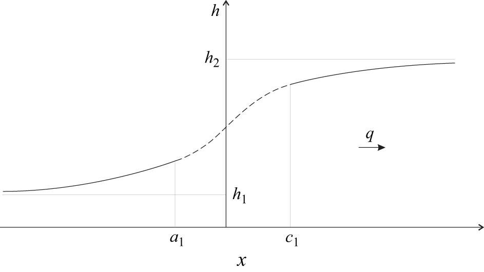
 (a1,c1)
 x
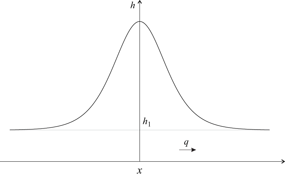
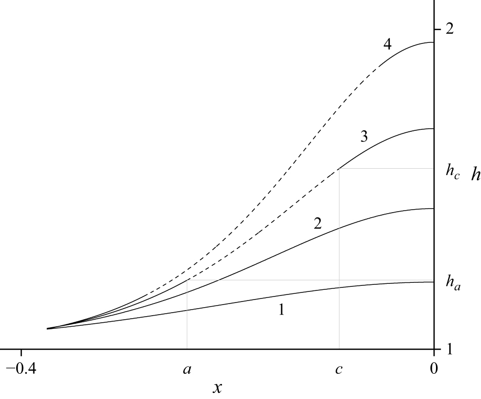
 h(x)
 x0=0
 δ=0.05
 q=1.1
 q=1.2
 q=1.3
 q=1.4
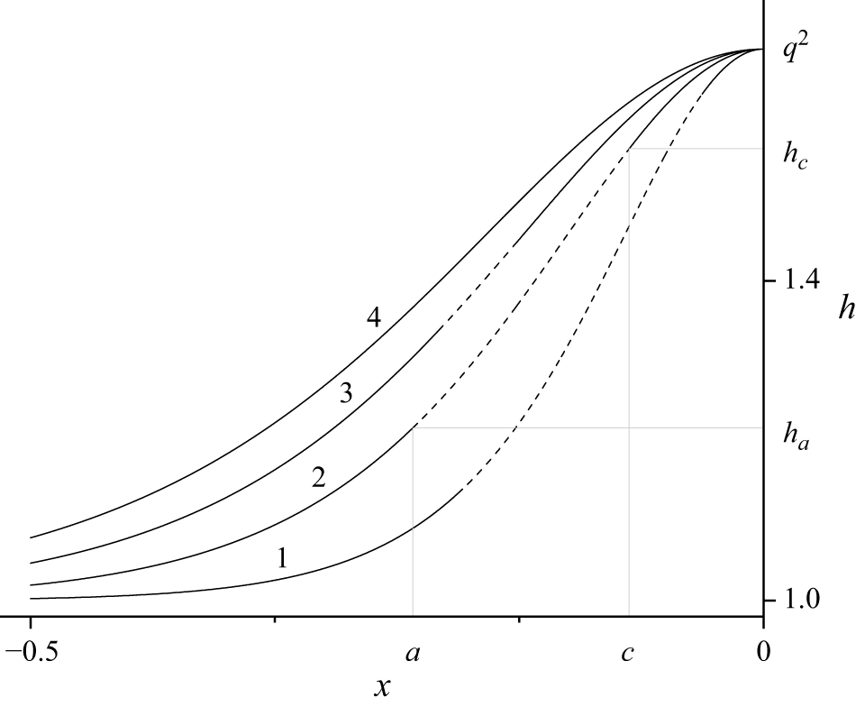
 h(x)
 x0=0
 q=1.3
 δ=0.025
 δ=0.05
 δ=0.075
 δ=0.1
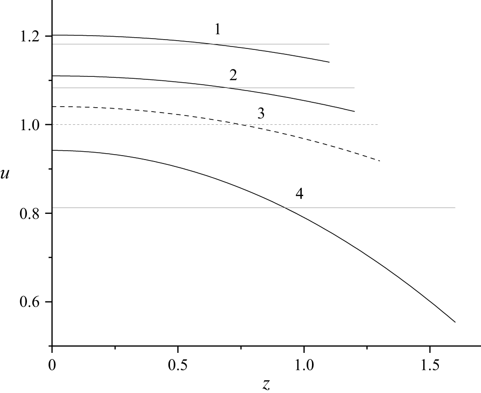
 u=u(z,h)
 z
 v
 x0=0
 δ=0.05
 q=1.3
 h=1.1
 h=1.2
 h=1.3
 h=1.6
 h=1.3
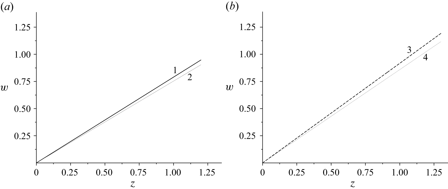
 z
 x0=0
 δ=0.05
 q=1.3
 h=1.2
 h=1.3
 h=1.3
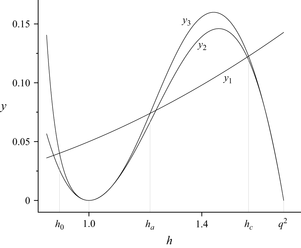
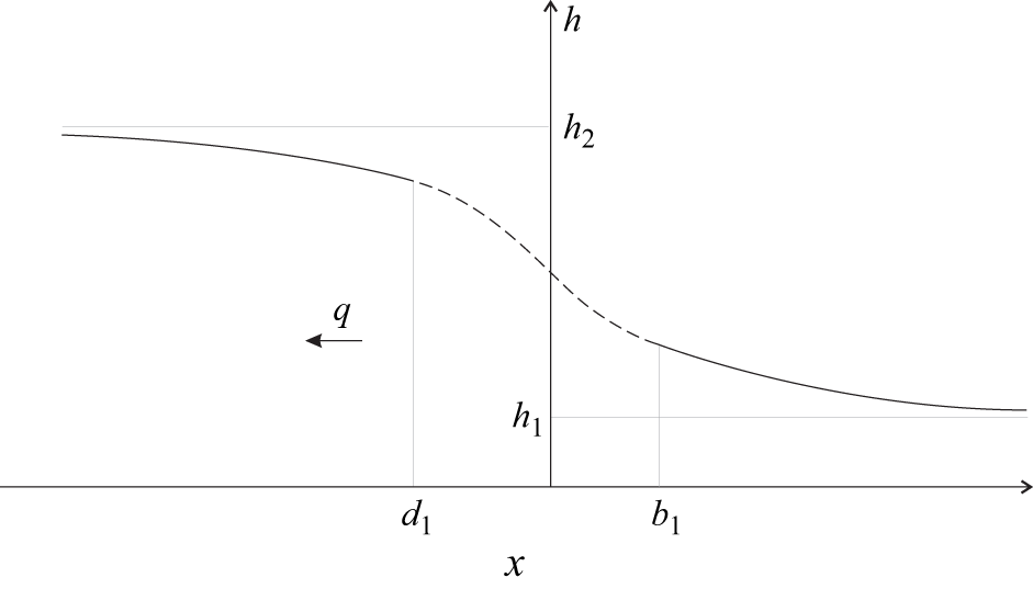
 (d1,b1)
 x
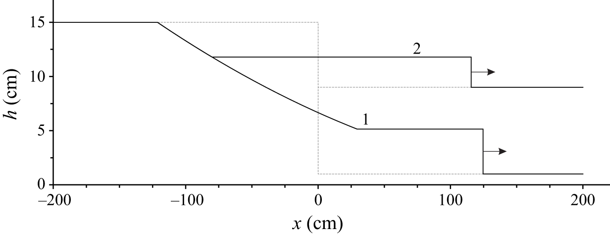
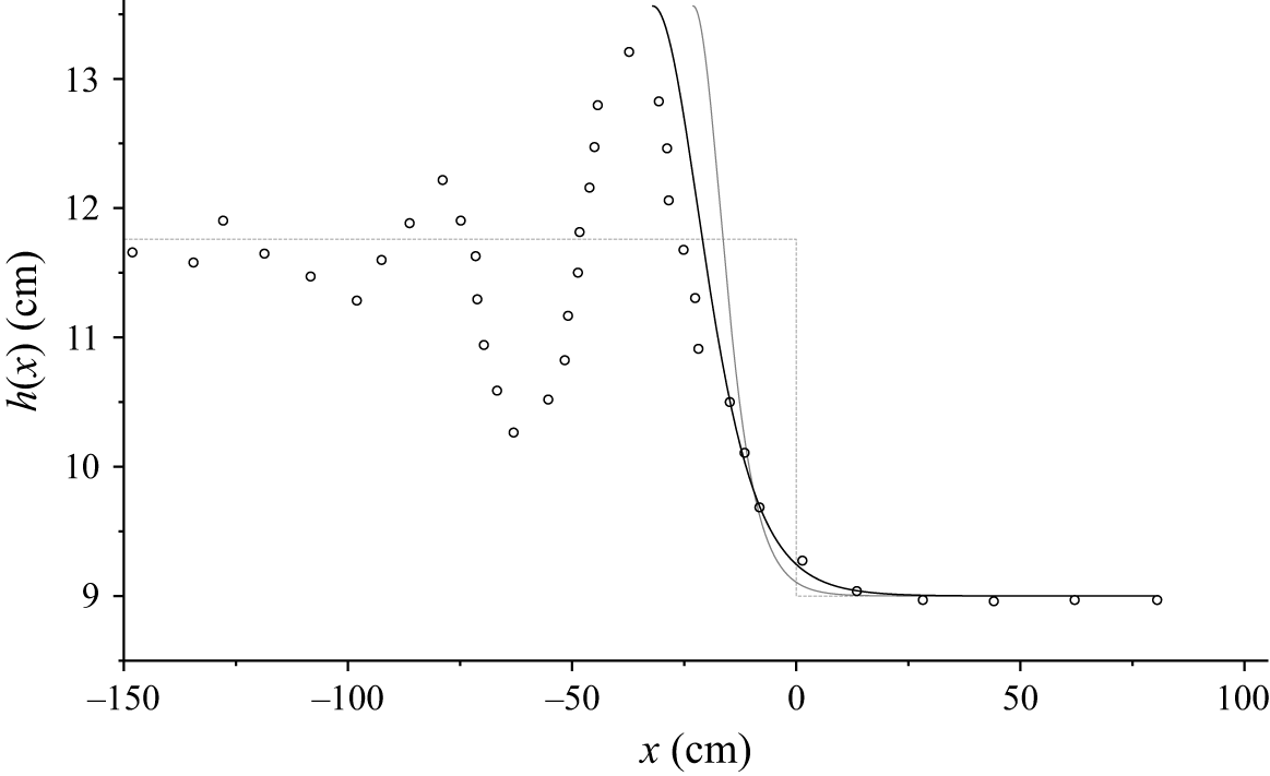
 α=0
 x~0=−23
 α=0.6
 x~0=−32
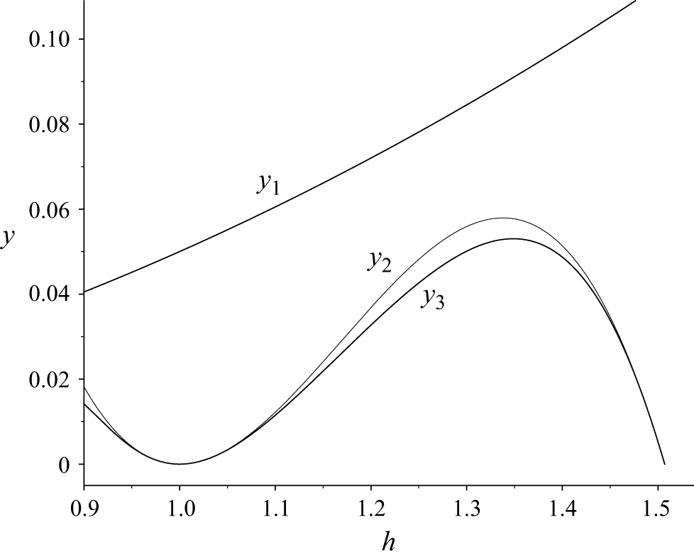
 yi(h)
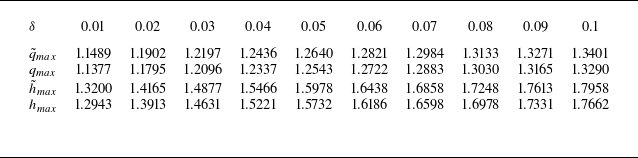
 δ
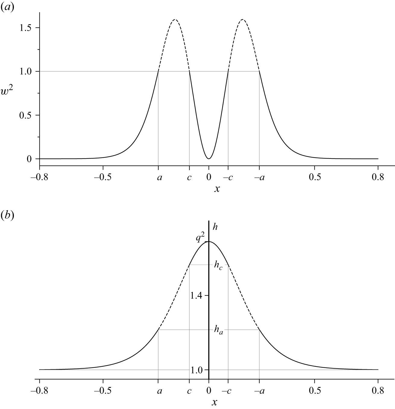
 w2(x,h(x))
 h(x)
 δ=0.05
 q=1.3
 a=−0.2393
 ha=1.2160
 c=−0.0918
 hc=1.5653
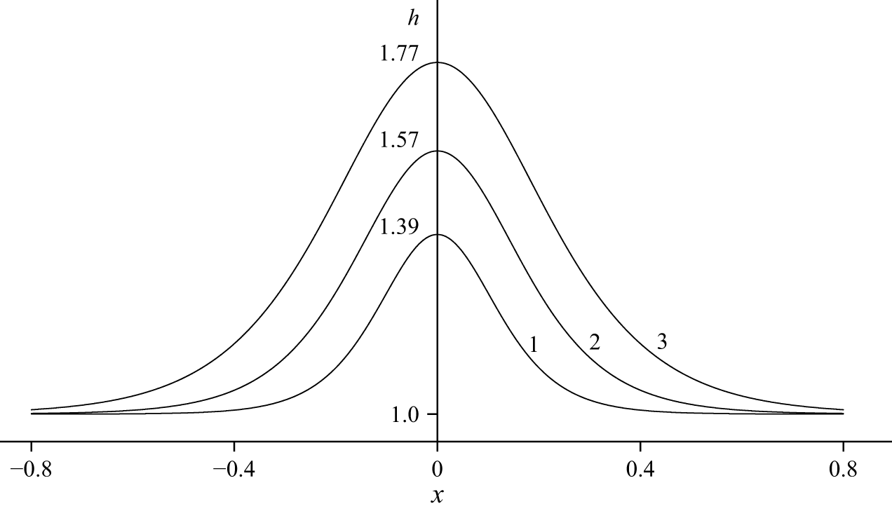
 δ=0.02
 δ=0.05
 δ=0.1
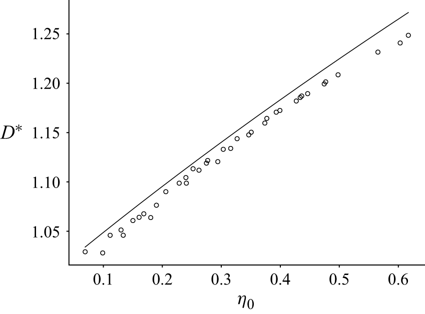
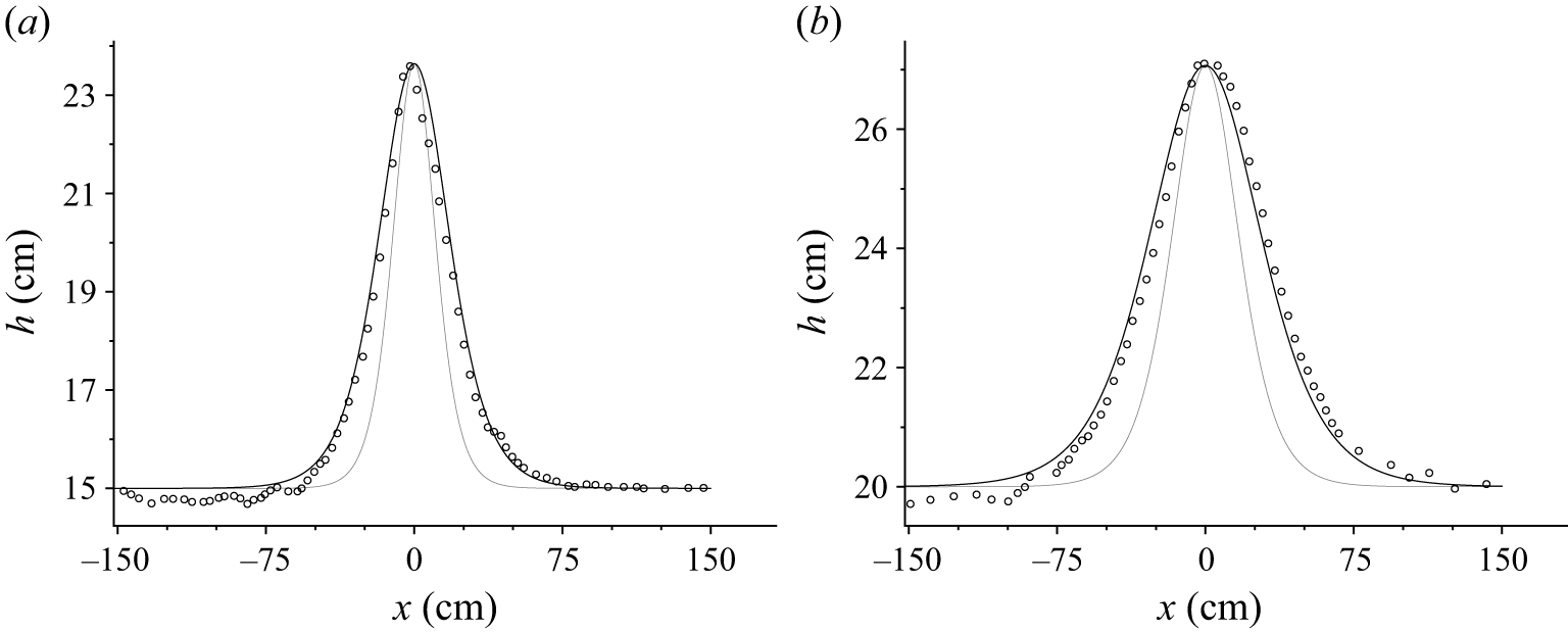
 α=1
 α=0.6
 a
 h1=15
 η0=8.64
 b
 h1=20
 η0=7.07


