1. Introduction
Compared with serial mechanisms with open-loop structures, parallel mechanisms stand out due to their higher stability and precision. Currently, numerous parallel mechanisms have successfully replaced serial mechanisms in multiple fields [Reference Saiki, Tadakuma, Watanabe, Takane, Nobutoki, Suzuki and Konyo1]. For example, the Stewart parallel mechanism [Reference You, Xi, Shen, Wang and Yang2–Reference Horoub, Hassan and Hawwa4], the Delta parallel mechanism [Reference Wu, Zhao, Cheng, Shi and Wang5–Reference Wu, Mei, Zhao and Niu8], the Tricept mechanism [Reference Ding and Wang9–Reference Siciliano10], and the Exechon mechanism [Reference Tang, Fang, Luo, Song and Zhang11–Reference Hu13] have all performed excellently in their respective application fields. However, it is worth noting that, despite the excellent performance indices of these widely used parallel mechanisms, they generally suffer from the problem of a single motion mode, which is somewhat restricted and difficult to adapt to the increasing demands of diverse tasks.
The reconfiguration mechanisms of reconfigurable parallel mechanisms are varied, encompassing the use of singular poses of parallel mechanisms [Reference Song, Xian, Huo and Qi14–Reference Deng, Zhang and Yan15], the relationships among constraint screws generated by limbs [Reference Liu, Li, Yao and Kong16–Reference Li, Wang and L.Liu17], and the implementation of variable joints [Reference Li, Gao, Wu, Sun and Shan18–Reference Li, Zhang and Tian20]. For example, Song [Reference Song, Xian, Huo and Qi14] cleverly employed the singular position of one limb of a parallel mechanism as a switch, designing a mechanism capable of transitioning between 3T and 3R motion modes. Similarly, Deng [Reference Deng, Zhang and Yan15] performed configuration synthesis of metamorphic and axisymmetric mechanisms utilizing singularity. By integrating deployment and locking functionalities into a single mechanism, they addressed, to some extent, the quality and trajectory problems of existing unfolded structures are solved. Liu [Reference Liu, Li, Yao and Kong16] introduced a type synthesis method for multi-mode mobile parallel mechanisms grounded in screw theory. They modified the axis position of the revolute joint within the driving limb to synthesize constraint screws, thereby facilitating the switching of parallel mechanisms among various motion modes.
While designing reconfigurable parallel mechanisms based on the singular poses of parallel mechanisms and the principles of screw theory demonstrates considerable universality and applicability, this approach necessitates a relatively high level of theoretical understanding from researchers. In contrast, the threshold for designing reconfigurable parallel mechanisms utilizing variable joints is comparatively lower.
In the past, some researchers have designed reconfigurable parallel mechanisms using novel variable joints. Lin [Reference Lin and Guo19] aimed at the poor adaptability of existing legged landers and designed a composite variable joint based on friction self-locking. Based on this composite variable joint, a reconfigurable parallel mechanism was designed. The designed reconfigurable parallel mechanism theoretically possesses an infinite number of locking configurations and exhibits high load-bearing capacity and shock resistance. Ye [Reference Ye, Chai and Zhang21] designed a reconfigurable parallel mechanism based on the phase changes of three variable-axis spherical joints, which is capable of switching among four different motion modes. It is worth noting that, under these motion modes with different numbers of DOFs, this configuration still maintains good motion transmission performance. Gan [Reference Gan, Dai and Liao22] invented two variable-morphology rT joint and rR joint and introduced methods for designing reconfigurable parallel mechanisms based on these two variable joints. Zhang [Reference Zhang, Dai and Fang23] proposed a variable-axis joint inspired by origami and applied this variable-axis joint to the design of reconfigurable parallel mechanisms. Carbonari [Reference Carbonari, Callegari, Palmieri and Palpacelli24–Reference Palpacelli, Carbonari, Palmieri and Callegari25] proposed a special lockable universal joint and, based on this joint, designed a class of reconfigurable parallel mechanisms capable of performing various motion types such as pure translation and pure rotation. Liu [Reference Liu and Wang26–Reference Liu, Wang and Pritschow27] proposed a class of spatial 3-DOF mechanisms with planar four-bar parallelogram joints and applied them to the design of parallel mechanisms.
Structural design and kinematic performance are two of the most critical research topics in the field of mechanism science. Structural design aims to create innovative structures that fulfill diverse functions, while the study of kinematic performance focuses on evaluating the performance of these designed structures and exploring optimization approaches to better adapt to various task requirements. In this paper, we propose a special limb based on a double-slider structure, which is integrated into the configuration design of a parallel mechanism, resulting in a reconfigurable parallel mechanism. Furthermore, this paper investigates key performance indices, including kinematics, workspace, and dexterity of the proposed mechanism.
In Section 2, the motion of the double slider mechanism is analyzed in detail, and a special structure is designed, which is applied to the configuration design of the parallel mechanism, and then a reconfigurable parallel mechanism is designed. In Section 3, the kinematic equations and Jacobian matrices of the proposed reconfigurable parallel mechanism are analyzed in depth. In Section 4, the performance indicators such as workspace, dexterity, and carrying capacity of the mechanism are studied in detail. Then, in Section5, an experimental prototype is built to verify the effectiveness and universality of the proposed special mechanism.
2. Design and analysis of a reconfigurable parallel mechanism
In this section, an innovative structure derived from the double-slider mechanism is introduced in detail, and it is skillfully applied to the configuration design of the parallel mechanism, so as to obtain a parallel mechanism with reconstruction ability. In this study, the motion modes of this particular structure were thoroughly investigated and it was shown that the structure is able to smoothly switch between three different motion modes, providing highly flexible reconfiguration characteristics for the parallel mechanism.
2.1 Design and analysis of special structures
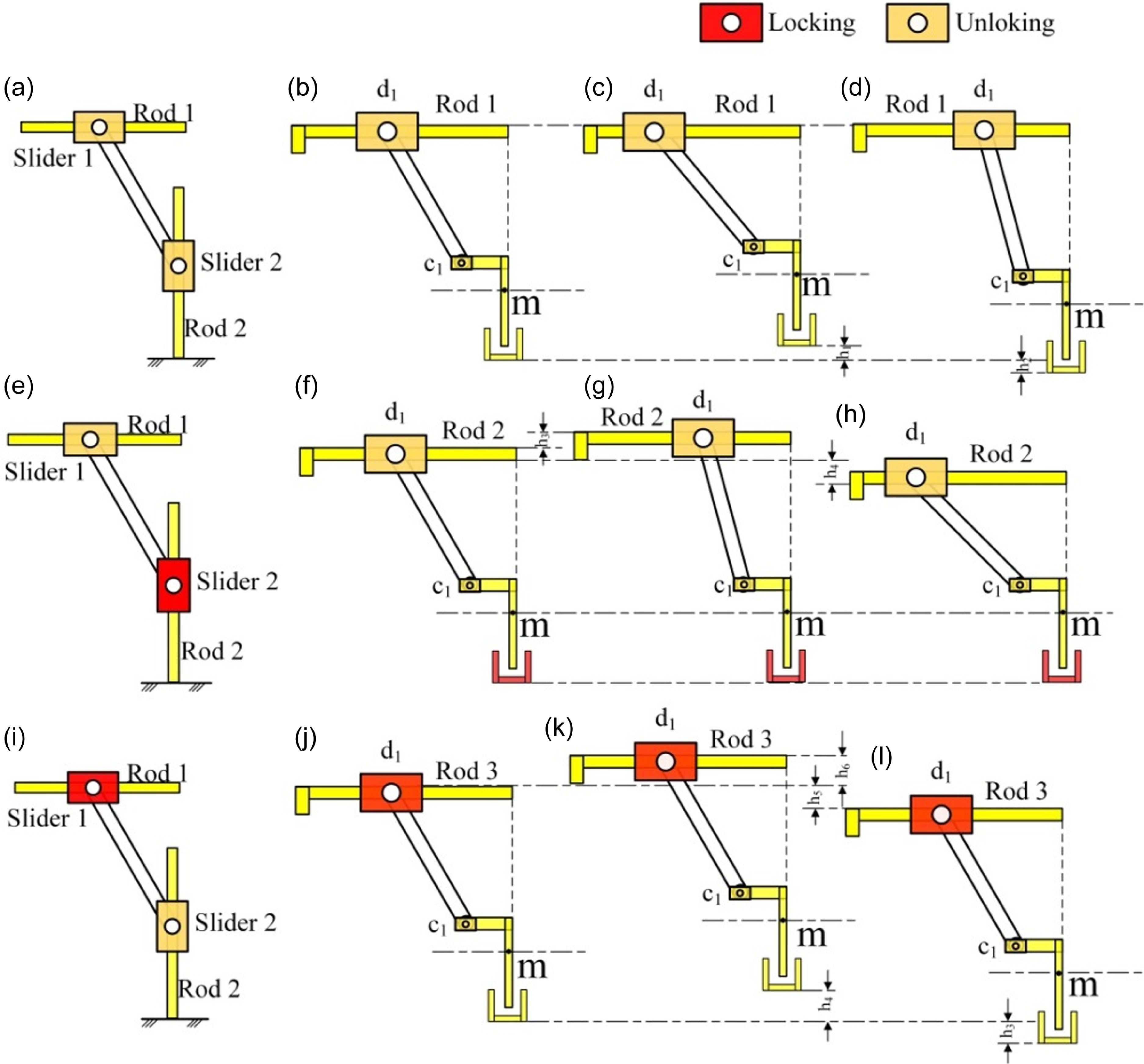
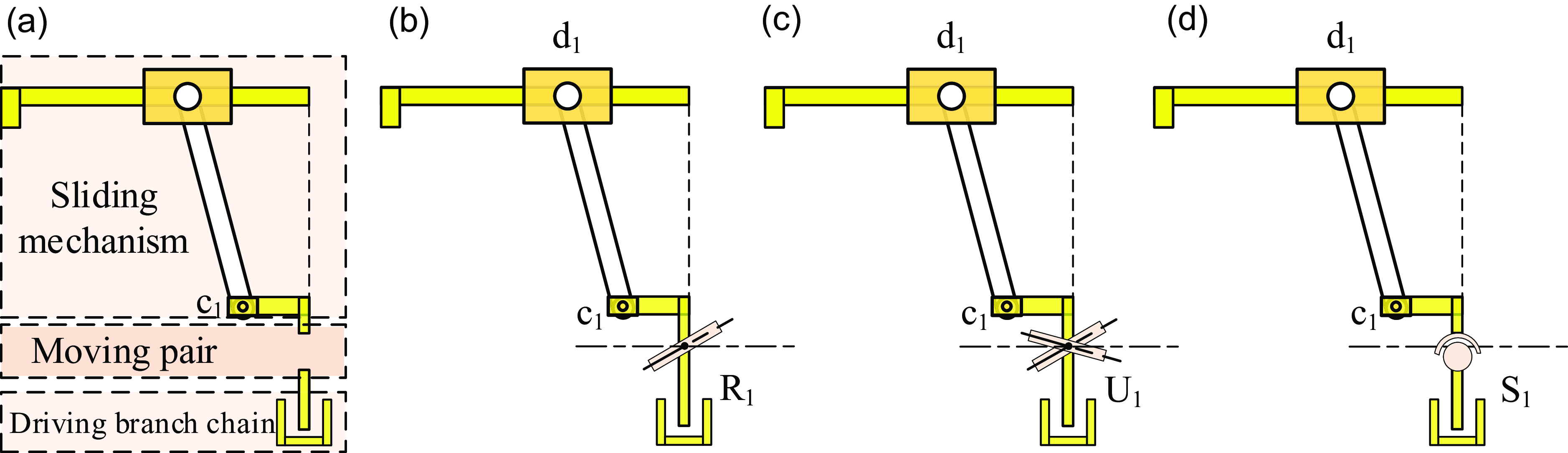
In this paper, we propose a special structure derived from a double-slider mechanism. Initially, we analyzed the movement patterns of the double-slider mechanism, as depicted in Figure 1(a), (e), and (i). Figure 1(a) presents the most common type of double-slider mechanism, where Rod 1 intersects Rod 2 perpendicularly and Rod 2 is fixed. The two sliders move linearly along Rod 1 and Rod 2, respectively, and are connected by a connecting rod. Figure 1(b)–(d) illustrates the motion rule of Figure 1(a). By comparing Figure 1(b)–(d), we observe that in this motion mode, although the position of point m varies along the Y-axis, when rod 1 is fixed, the Y-axis position coordinates of point d1 remain constant. In Figure 1(e), slider 2 is locked on Rod 2, causing slider 1 to be locked on Rod 1 under the combined action of the connecting rod and Rod 1, and they cannot move relative to each other. Figure 1(f)–(h) shows the motion law of Figure 1(e). When Rod 1 is moved, the position of point m remains unchanged, while the Y-axis coordinates of point d1 can be altered. In Figure 1(i), slider 1 is fixed on Rod 1, and slider 2 can move freely on Rod 2, but simultaneously, it will drive Rod 1 to move, resulting in an accompanying motion. As can be seen from Figure 1(j)–(l), the coordinate changes of point m and point d1 in the Y-direction are consistent. Notably, the main distinction among the three motion modes exhibited by the special structure in Figure 1 lies in the variation of position in the Y-axis direction. This ingenious design endows the special structure with a rich variety and flexibility in motion modes. To further enhance the flexibility of the special structure, based on the special structure shown in Figure 1, different motion pairs are added to expand the applicable scenarios of the special structure, as shown in Figure 2.
Schematic diagram of motion analysis of double slider mechanism.

Schematic structure of special branch chain based on special structure.

It can be observed from Figure 2(a) that on the basis of the special structure shown in Figure 1, the common motion pair is introduced at the m point. As shown in Figure 2(b), a rotating pair is added; in Figure 2(c), a universal joint is added; and in Figure 2(d), a ball pair is added. The original special structure is made to evolve into a unique branch suitable for the design of the parallel mechanism by these changes. The branch chain has multiple motion modes, which in turn gives the parallel mechanism a rich choice of motion modes. It is worth mentioning that the key to switching the motion mode is located in the specific motion state of the two sliders. One slider in the upper slider mechanism and the driving branch below are corresponded to by these two sliders.
2.2 Design of reconfigurable parallel mechanism
When the mechanism is in different modes of motion, we often expect the motion screw of the mechanism to be:
 \begin{equation} \left\{{}^{j}{\$ }{}\left| \left({}^{j}{\$ }{_{1}^{}},{}^{j}{\$ }{_{2}^{}},\cdots {}^{j}{\$ }{_{f}^{}}\right)\right.\right\} \end{equation}
In Eq. (1), j represents the j-th motion mode, and f is the number of DOFs.
The constrained screw in different motion modes can be obtained as follows according to the reciprocal product formula in screw theory:
 \begin{equation} \left\{{}^{j}{\$ }{_{}^{r}}\left| {}^{j}{\$ }{_{1}^{r}},\right.{}^{j}{\$ }{_{2}^{r}},{}^{j}{\$ }{_{3}^{r}}\cdots {}^{j}{\$ }{_{6-f}^{r}}\right\} \end{equation}
The constrained screws in Eq. (2) are all independent and uncorrelated. In many cases, the number of constrained screws in a parallel mechanism exceeds the number of independent constrained screws due to the presence of linearly correlated constrained screws. Such a parallel mechanism is referred to as an over-constrained parallel mechanism.
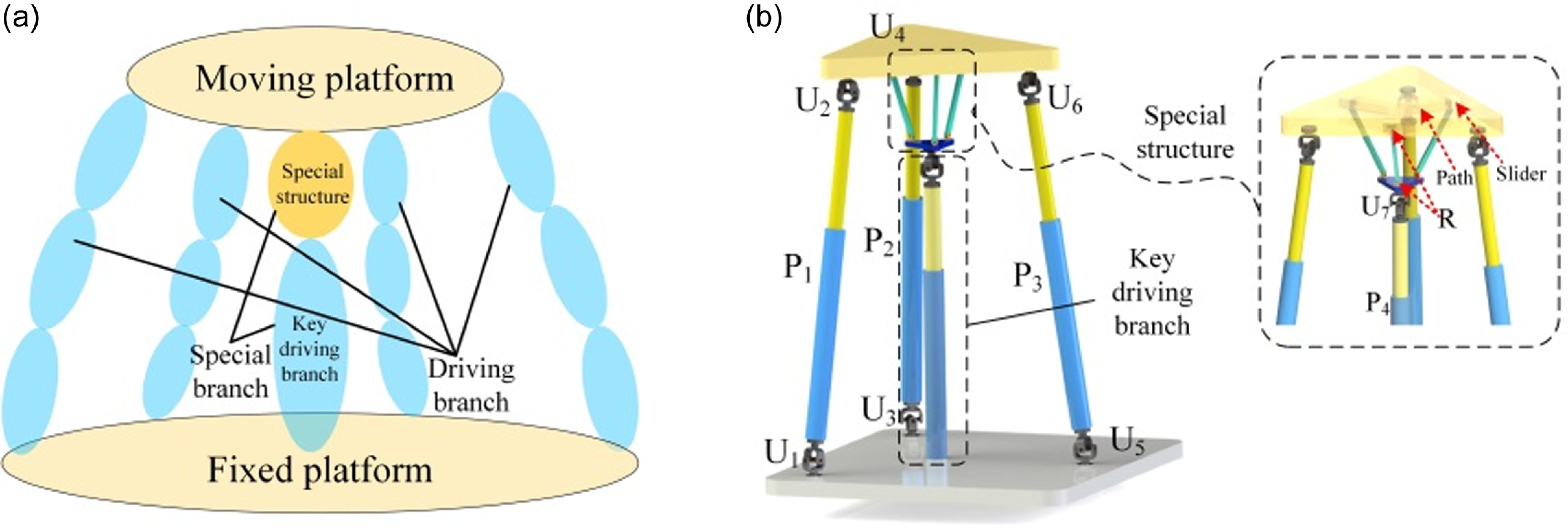
In this paper, a parallel mechanism with reconfiguration characteristics is constructed based on the designed special branch chain, as shown in Figure 3. Figure 3(a) shows the design concept of the reconfigurable parallel mechanism, Figure 3(b) shows its 3D model (where R represents the rotating pair, U represents the universal joint, and P represents the moving pair).
Schematic diagram of 3D model of reconfigurable parallel mechanism.

It is clear from Figure 3(b) that the proposed reconfigurable parallel mechanism is mainly composed of a special branch chain and a 3UPU parallel mechanism. The rotational axes of the two U pairs in the peripheral UPU branch are parallel to the fixed platform. The design of the special branch chain is inspired by Figure 3(c), but the slider mechanism part is adjusted: in order to adapt to the equilateral triangular shape of the moving platform of the 3UPU parallel mechanism, three slider-mechanisms are used, and they are uniformly distributed at 120 degrees in space. This change does not affect the motion pattern of the special structure shown in Figure 1.
2.3 Motion mode analysis of reconfigurable parallel mechanism
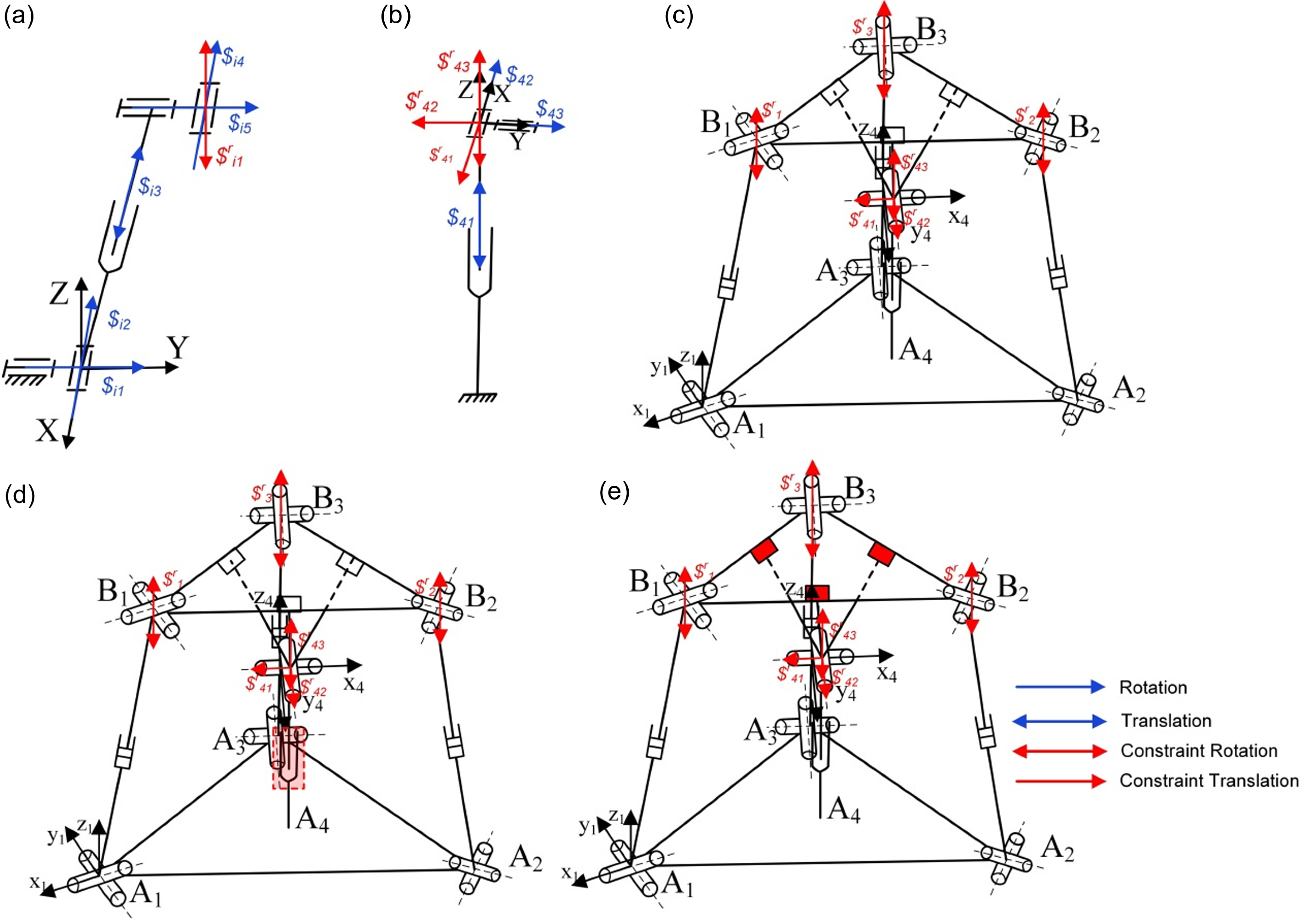
According to Figs. 1 and 3, three motion modes are possessed by the reconfigurable parallel mechanism proposed in this paper. The mechanism schematic diagram of the reconfigurable parallel mechanism is established, as illustrated in Figure 4. Based on the screw theory, the constraints of the screw are analyzed.
Mechanism diagram of reconfigurable parallel mechanism.

The reconfigurable parallel mechanism designed in this paper is composed of a 3UPU parallel mechanism and a special branch chain, which have three motion modes, respectively. Figure 4(a) and (b) shows the mechanism diagrams of the two types of branch chains, respectively, while Figure 4(c) to (e) depicts the mechanism diagrams of the three modes of motion, where the parts highlighted in red indicate that they are locked. First, the constraint spiral generated by each branch chain is analyzed. The establishment of the coordinate system is shown in Figure 4 (a) and (b) :
 \begin{equation} \left\{\begin{array}{l} \$ _{11}=\left(010\,;\,000\right)\\ \$ _{12}=\left(100\,;\,000\right)\\ \$ _{13}=\left(000\,;\,0e_{3}d_{3}\right)\\ \$ _{14}=\left(100\,;\,0e_{3}d_{4}\right)\\ \$ _{15}=\left(010\,;\,d_{5}00\right) \end{array}\right. \end{equation}
According to the reciprocal product formula in the screw theory, the constraints of UPU branching can be calculated as follows:
 \begin{equation} {\$ ^{\mathrm{r}}}_{11}=\left(000\,;\,001\right) \end{equation}
According to Eq. (4), the constraint helix of the UPU in this paper is a constraint couple parallel to the Z-axis, that is, the branch chain limits the rotational DOFs of the parallel mechanism around the Z-axis. Similarly, the analysis of Figure 4 (b) shows that the branch chain produces two binding forces and a constraint couple, which constrain the rotational DOFs around the Z-axis and the moving DOFs along the X-axis and Y-axis.
Without considering the special branch, the number of DOFs of the 3UPU parallel mechanism is 5, which are the DOFs of movement along the X, Y, and Z axes and the DOFs of rotation around the X and Y axes. If the special structure is considered, there are three different motion modes.
Motion Mode 1: The mechanism schematic for this mode is presented in Figure 4(c). Here, the special structure’s state is identical to that in Figure 1(a). By adjusting the key branch’s expansion and contraction length, the universal joint’s position along the Z-axis can be adjusted without altering the moving platform, thus shifting the moving platform’s rotation center. Once the key branch reaches a predefined position, both the key branch and the slider on the moving platform are locked, endowing the parallel mechanism with two rotational DOFs around the x4 and y4-axes. Hence, Motion Mode 1 can be termed the 2R mode.
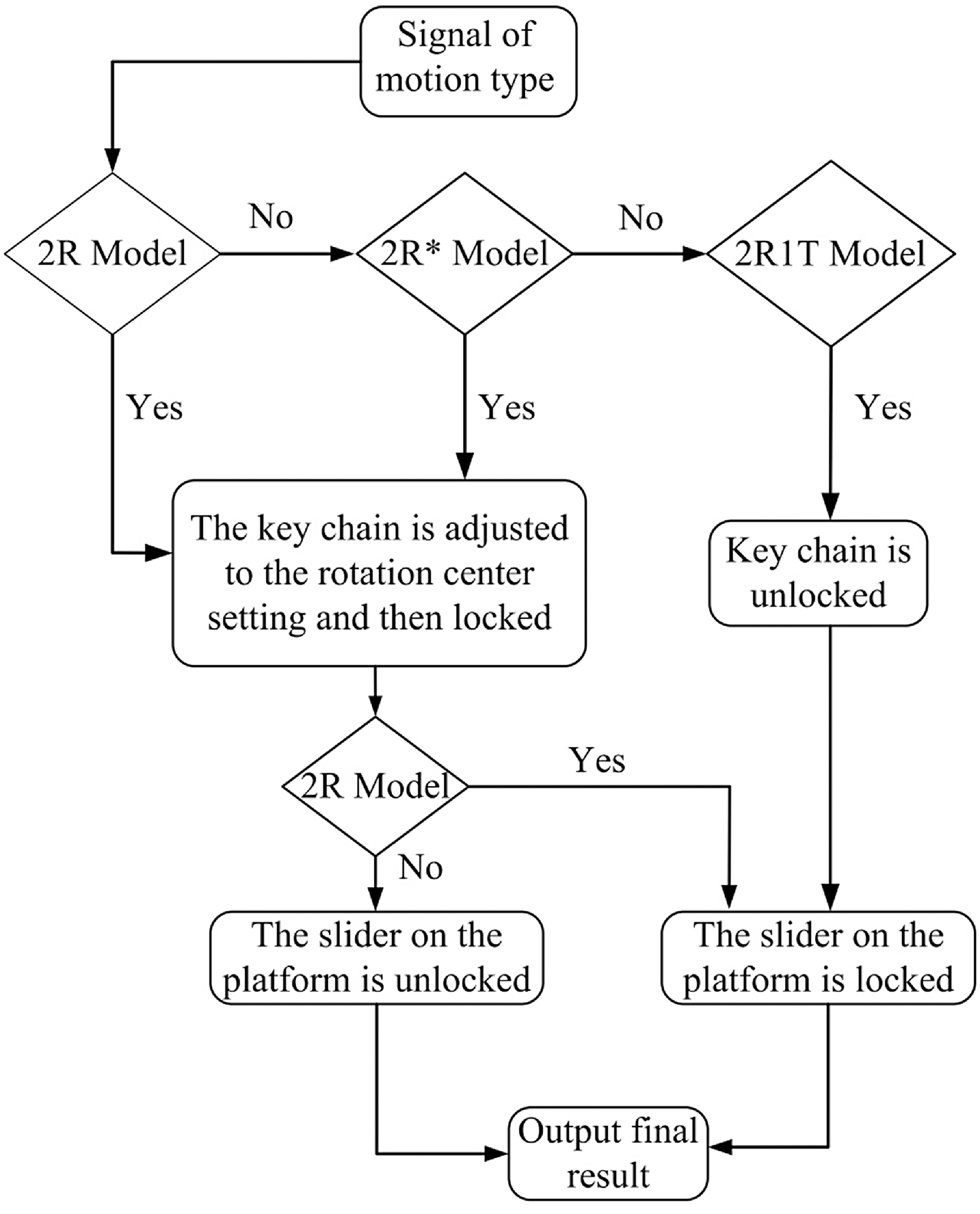
Movement mode switching flow diagram.

Motion Mode 2: The mechanism schematic for Motion Mode 2 is depicted in Figure 4(d), and the state of its special structure corresponds to that in Figure 1(e). Similar to the mechanism diagram of Motion Mode 1, the only distinction is that when the key branch is extended or retracted to a preset length, only the key branch itself is locked, rather than the slider on the moving platform. Based on Motion Mode 1, the parallel mechanism gains an additional degree of freedom of movement in the z4- axis direction. Notably, this freedom of movement is not provided by the entire parallel mechanism but is contributed by the special structure. Thus, Motion Mode 2 is designated as the 2R* mode.
Motion Mode 3: The schematic diagram of the mechanism of Motion Mode 3 is presented in Figure 4(e), and the state of its special structure is consistent with Figure 1(i). At this time, only the position of the slider on the moving platform is locked, and no restrictions are placed on the key branches. In this mode, the freedom of movement along the z4-axis direction and the freedom of rotation around the x4 and y4 axes are possessed by the parallel mechanism. Motion Mode 3 is named as the 2R1T mode. Combined with the above three motion modes, the switching mode between different motion modes can be shown in Figure 5.
3. Kinematics analysis of reconfigurable parallel mechanism
3.1 Inverse kinematics analysis
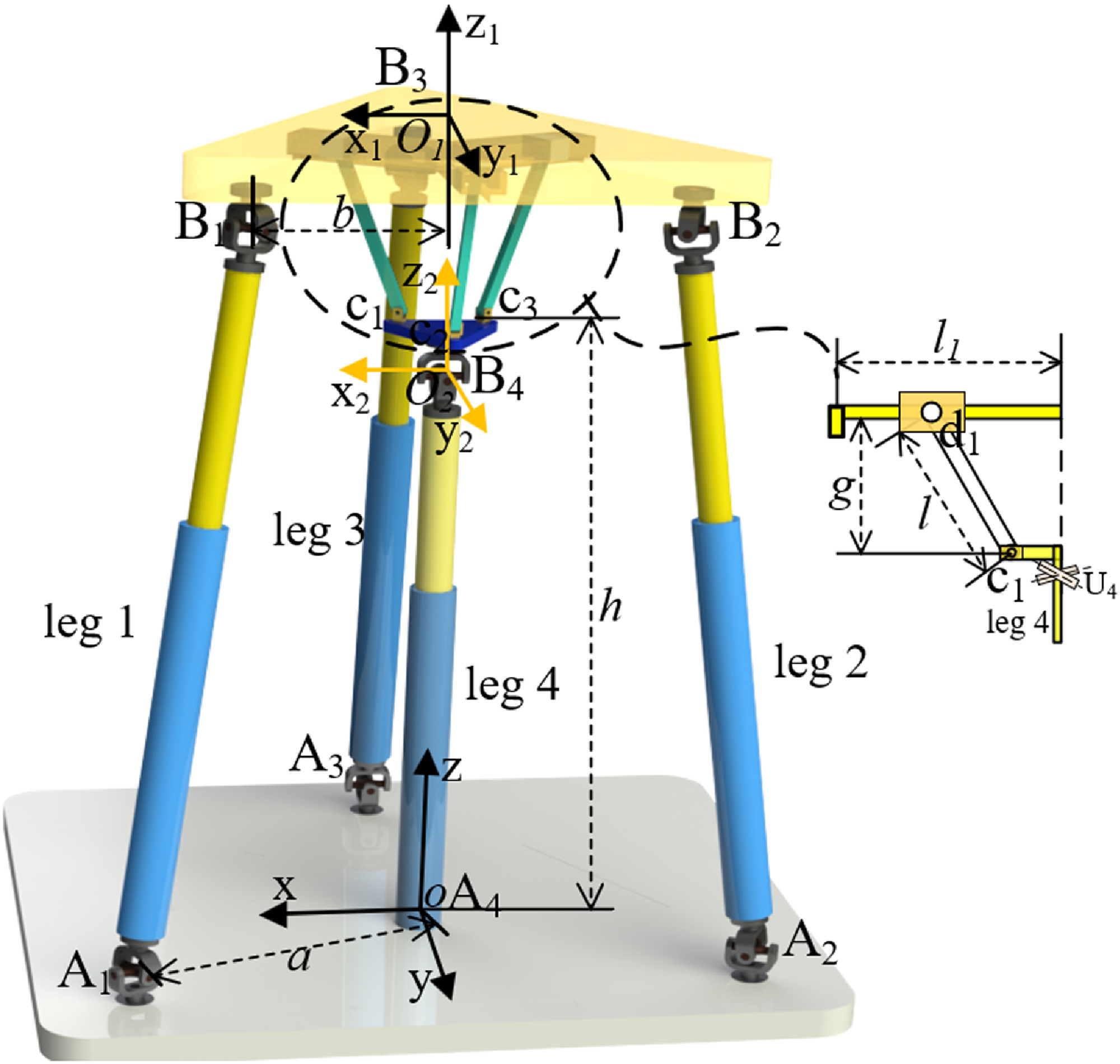
To conduct a thorough analysis of the kinematic characteristics of the reconfigurable parallel mechanism presented in this paper, coordinate systems are established for both the moving platform and the fixed platform, as illustrated in Figure 6. The fixed platform A1A2A3 and the moving platform B1B2B3 are configured as equilateral triangles, with the origin O of the fixed coordinate system and the origin O 1 of the moving coordinate system positioned at the centroids of their respective platforms. Each endpoint Ai on the fixed platform is located at a distance a from the origin O of the fixed coordinate system, while each endpoint Bi on the moving platform is situated at a distance b from the origin O 1 of the moving coordinate system. The distance between point O 3 and the origin O of the fixed coordinate system is denoted as h, the distance between O 3 and the moving platform is represented as g, and the length of segment c1d1 in the special structure is defined as l.
Schematic diagram of establishing coordinate system.

The rotational DOFs of the reconfigurable parallel mechanism designed in this paper are all rotational DOFs about the x2-axis and the y2-axis. Therefore, the coordinate change between the moving platform coordinate system and the fixed coordinate system adopts the roll-pitch-yaw method [Reference Liu, Xu, Shen, Shan and Yang28], then the change matrix R between them is expressed as:
 \begin{equation} R=R\mathit{ot}\left(\mathit{y},\,\beta \right)\times R\mathit{ot}\left(\mathit{x},\,\alpha \right)=\left[\begin{array}{l} \mathit{c}\beta \mathit{s}\alpha \mathit{s}\beta \mathit{c}\alpha \mathit{s}\beta \\ \mathit{0}\mathit{c}\alpha \mathit{-}\mathit{s}\alpha \\ \mathit{-}\mathit{s}\beta \mathit{s}\alpha \mathit{c}\beta \mathit{c}\alpha \mathit{c}\beta \end{array}\right] \end{equation}
where c represents cos and s represents sin.
The endpoint coordinates of each branch on a fixed platform under a fixed coordinate system are
 \begin{equation} \left\{\begin{array}{l} A_{1}=\left[\sqrt{3}\mathit{a}/2\mathit{a}/20\right]^{T}\\ A_{2}=\left[-\sqrt{3}\mathit{a}/2\mathit{a}/20\right]^{T}\\ A_{3}=\left[0\mathit{a}0\right]^{T} \end{array}\right. \end{equation}
The endpoint coordinates of each branch on the moving platform under the moving coordinate system are
 \begin{equation} \left\{\begin{array}{l} B_{1}=\left[\sqrt{3}\mathit{b}/2\mathit{b}/20\right]^{T}\\ B_{2}=\left[-\sqrt{3}\mathit{b}/2\mathit{b}/20\right]^{T}\\ B_{3}=\left[0\mathit{b}0\right]^{T} \end{array}\right. \end{equation}
The coordinates of the endpoints of each branch chain on the moving platform in a fixed coordinate system are
 \begin{equation} B_{\mathit{i}}^{\sim }=RB_{i} \end{equation}
Notably, the coordinates of the aforementioned endpoints remain unchanged across the three motion modes. This is because no alterations have been made to the 3UPU parallel mechanism. The sole difference lies in the expression of the O 1 point within the fixed coordinate system.
 \begin{equation} \left\{\begin{array}{l} O_{1}^{1}=\left[g\mathit{c}\alpha \mathit{s}\beta -\mathit{gs}\alpha \textit{ gc}\alpha \mathit{c}\beta \mathit{+}\mathit{h}\right]^{T}\\[3pt] O_{1}^{2}=\left[\left(g+Z\right)\mathit{c}\alpha \mathit{s}\beta -\left(g+Z\right)\mathit{s}\alpha \left(g+Z\right)\mathit{c}\alpha \mathit{c}\beta \mathit{+}\mathit{h}\right]^{T}\\[3pt] O_{1}^{3}=\left[g\mathit{c}\alpha \mathit{s}\beta -\mathit{gs}\alpha \textit{ gc}\alpha \mathit{c}\beta \mathit{+}\mathit{h}\mathit{+}\mathit{Z}\right]^{T} \end{array}\right. \end{equation}
In Eq. (9), the three coordinates of point O
1
correspond to the 2R mode, 2R* mode and 2R1T mode, respectively. Where,
 $\alpha$
and
 $\beta$
represent the rotation angles of the moving platform around the x2 and y2 axes, respectively, g represents the distance between the moving platform and the O
2
point, h represents the distance between the O
2
point and the origin of the fixed coordinate system, and Z represents the displacement of the moving platform in the direction of the z2 axis.
The vector expression of AiBi in o-xyz can be obtained by closed loop vector method.
 \begin{equation} A_{\mathit{i}}^{\mathit{j}}B_{\mathit{i}}^{\mathit{j}}=OO_{2}+O_{2}O_{1}^{\mathit{j}}+B_{\mathit{i}}^{\sim }-OA_{\mathit{i}} \end{equation}
The formula for calculating the length of each branch chain can be derived from Eq. (10) as follows:
 \begin{equation} L_{\mathit{i}}^{\mathit{j}}=\left\| A_{\mathit{i}}^{\mathit{j}}B_{\mathit{i}}^{\mathit{j}}\right\| \end{equation}
where j represents the motion mode, the 2R mode corresponds to j = 1, the 2R* mode corresponds to j = 2, and the 2R1T mode corresponds to j = 3.
Inverse kinematics equation of 2R mode:
 \begin{equation*} L_{1}^{1}=\left[\begin{array}{l} \frac{\sqrt{3}}{2}\mathit{bc}\beta +\frac{\mathit{b}}{2}\mathit{s}\beta \mathit{s}\alpha +\mathit{gc}\alpha \mathit{s}\beta -\frac{\sqrt{3}}{2}\mathit{a}\\ \frac{\mathit{b}}{2}\mathit{c}\alpha -\mathit{gs}\alpha -\frac{\mathit{a}}{2}\\ -\frac{\sqrt{3}}{2}\mathit{bs}\beta +\frac{\mathit{b}}{2}\mathit{c}\beta \mathit{s}\alpha +\mathit{gc}\alpha \mathit{c}\beta +\mathit{h} \end{array}\right] L_{2}^{1}=\left[\begin{array}{l} -\frac{\sqrt{3}}{2}\mathit{bc}\beta +\frac{\mathit{b}}{2}\mathit{s}\beta \mathit{s}\alpha +\mathit{gc}\alpha \mathit{s}\beta +\frac{\sqrt{3}}{2}\mathit{a}\\ \frac{\mathit{b}}{2}\mathit{c}\alpha -\mathit{gs}\alpha -\frac{\mathit{a}}{2}\\ \frac{\sqrt{3}}{2}\mathit{bs}\beta +\frac{\mathit{b}}{2}\mathit{c}\beta \mathit{s}\alpha +\mathit{gc}\alpha \mathit{c}\beta +\mathit{h} \end{array}\right] \end{equation*}
 \begin{align} L_{3}^{1}=\left[\begin{array}{l} -\mathit{bs}\alpha \mathit{s}\beta +\mathit{gc}\alpha \mathit{s}\beta \\ -\mathit{bc}\alpha -\mathit{gs}\alpha +\mathit{a}\\ -\mathit{bs}\alpha \mathit{c}\beta +\mathit{gc}\alpha \mathit{c}\beta +\mathit{h} \end{array}\right] \end{align}
Inverse kinematics equation of 2R* mode:
 \begin{align} L_{1}^{2}=\left[\begin{array}{l} \frac{\sqrt{3}}{2}\mathit{bc}\beta +\frac{\mathit{b}}{2}\mathit{s}\beta \mathit{s}\alpha +\left(\mathit{g}\mathit{+}\mathit{Z}\right)\mathit{c}\alpha \mathit{s}\beta -\frac{\sqrt{3}}{2}\mathit{a}\\ \frac{\mathit{b}}{2}\mathit{c}\alpha -\left(\mathit{g}\mathit{+}\mathit{Z}\right)\mathit{s}\alpha -\frac{\mathit{a}}{2}\\ -\frac{\sqrt{3}}{2}\mathit{bs}\beta +\frac{\mathit{b}}{2}\mathit{c}\beta \mathit{s}\alpha +\left(\mathit{g}\mathit{+}\mathit{Z}\right)\mathit{c}\alpha \mathit{c}\beta +\mathit{h} \end{array}\right] L_{3}^{2}=\left[\begin{array}{l} -\mathit{bs}\alpha \mathit{s}\beta +\left(\mathit{g}\mathit{+}\mathit{Z}\right)\mathit{c}\alpha \mathit{s}\beta \\ -\mathit{bc}\alpha -\left(\mathit{g}\mathit{+}\mathit{Z}\right)\mathit{s}\alpha +\mathit{a}\\ -\mathit{bs}\alpha \mathit{c}\beta +\left(\mathit{g}\mathit{+}\mathit{Z}\right)\mathit{c}\alpha \mathit{c}\beta +\mathit{h} \end{array}\right] \\ \nonumber L_{2}^{2}=\left[\begin{array}{l} -\frac{\sqrt{3}}{2}\mathit{bc}\beta +\frac{\mathit{b}}{2}\mathit{s}\beta \mathit{s}\alpha +\left(\mathit{g}\mathit{+}\mathit{Z}\right)\mathit{c}\alpha \mathit{s}\beta +\frac{\sqrt{3}}{2}\mathit{a}\\ \frac{\mathit{b}}{2}\mathit{c}\alpha -\left(\mathit{g}\mathit{+}\mathit{Z}\right)\mathit{s}\alpha -\frac{\mathit{a}}{2}\\ \frac{\sqrt{3}}{2}\mathit{bs}\beta +\frac{\mathit{b}}{2}\mathit{c}\beta \mathit{s}\alpha +\left(\mathit{g}\mathit{+}\mathit{Z}\right)\mathit{c}\alpha \mathit{c}\beta +\mathit{h} \end{array}\right] \end{align}
Inverse kinematics equation of 2R1T mode:
 \begin{align} L_{1}^{3}=\left[\begin{array}{l} \frac{\sqrt{3}}{2}\mathit{bc}\beta +\frac{\mathit{b}}{2}\mathit{s}\beta \mathit{s}\alpha +\mathit{gc}\alpha \mathit{s}\beta -\frac{\sqrt{3}}{2}\mathit{a}\\ \frac{\mathit{b}}{2}\mathit{c}\alpha -\mathit{gs}\alpha -\frac{\mathit{a}}{2}\\ -\frac{\sqrt{3}}{2}\mathit{bs}\beta +\frac{\mathit{b}}{2}\mathit{c}\beta \mathit{s}\alpha +\mathit{gc}\alpha \mathit{c}\beta +\mathit{h}\mathit{+}\mathit{Z} \end{array}\right] L_{2}^{3}=\left[\begin{array}{l} -\frac{\sqrt{3}}{2}\mathit{bc}\beta +\frac{\mathit{b}}{2}\mathit{s}\beta \mathit{s}\alpha +\mathit{gc}\alpha \mathit{s}\beta +\frac{\sqrt{3}}{2}\mathit{a}\\ \frac{\mathit{b}}{2}\mathit{c}\alpha -\mathit{gs}\alpha -\frac{\mathit{a}}{2}\\ \frac{\sqrt{3}}{2}\mathit{bs}\beta +\frac{\mathit{b}}{2}\mathit{c}\beta \mathit{s}\alpha +\mathit{gc}\alpha \mathit{c}\beta +\mathit{h}\mathit{+}\mathit{Z} \end{array}\right] \\ \nonumber L_{3}^{3}=\left[\begin{array}{l} -\mathit{bs}\alpha \mathit{s}\beta +\mathit{gc}\alpha \mathit{s}\beta \\ -\mathit{bc}\alpha -\mathit{gs}\alpha +\mathit{a}\\ -\mathit{bs}\alpha \mathit{c}\beta +\mathit{gc}\alpha \mathit{c}\beta +\mathit{h}\mathit{+}\mathit{Z} \end{array}\right] L_{4}^{3}=\left[\begin{array}{l} 0\\ 0\\ Z+\mathit{h} \end{array}\right] \end{align}
3.2 Positive kinematics analysis
Solving the inverse kinematics equations of parallel mechanisms is generally uncomplicated. Nevertheless, owing to the abundant branches, degrees of freedom (DOFs), and inherent structural variables in these mechanisms, the forward kinematics equations are more arduous to analyze and solve compared to their inverse counterparts. To boost the efficiency of solving the forward kinematics problem for parallel mechanisms, numerous researchers have delved into diverse methods. For instance, genetic algorithms [Reference Wu29] and particle swarm optimization algorithms [Reference Wang and Zhang30] have been employed to mitigate the complexity in deriving the forward kinematics equations.
The least square method is used to build the optimization objective function.
 \begin{equation} F=\sqrt{\sum _{\mathit{i}=1}^{\mathit{n}}\left| L_{\mathit{i}}-\mathit{q}_{\mathit{i}}\right| ^{2}} \end{equation}
In Eq. (13), L is the rod length solved based on the inverse kinematics equation, and q is the rod length we input. Through the optimization algorithm, the pose parameters of the moving platform can be solved. Based on genetic algorithm, the positive kinematics of the parallel mechanism is solved by giving the required structural parameter values. Here, the inverse kinematics equation of the 2R1T model is selected for verification. Where the given structural parameters:
 $\mathit{a}=150\mathit{mm}\mathrm{,}\,\mathit{b}\mathit{=}\mathit{100}\mathit{mm}\mathrm{,}\,\mathit{h}\mathit{=}\mathit{180}\mathit{mm}\mathrm{,}\,\mathit{g}\mathit{=}\mathit{70}\mathit{mm}$
. The key parameters in genetic algorithm are set to: number of variables 3; variable range is set to
 $[-0.5\pi 0.5\pi ]$
and
 $[-40\textit{mm }\mathit{40}\mathit{mm}]$
; population size: 50, elite count: 0.25; crossover fraction: 0.8; mutation: 0.01; generations: 100.
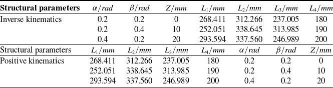
By integrating the structural parameters of the mechanism and the pose parameters of the moving platform into Eq. (11), the length of each driving branch chain rod can be precisely determined. Subsequently, the rod lengths derived from solving the inverse kinematics equation are substituted into Eq. (15) to calculate the pose parameters of the moving platform accurately. Finally, these calculated pose parameters are compared with the initial input pose parameters of the inverse kinematics equation. This comparison serves to validate the efficacy of the genetic algorithm in solving the position kinematics problem of the parallel mechanism. The verification results are presented in Table I:
Positive kinematics verification result.

3.3 Solution of Jacobian matrix
The velocity Jacobian matrix of the parallel mechanism describes the velocity relationship between the joints of the branch chain of the mechanism. There are various methods to solve the Jacobian matrix. In this paper, differential method is adopted to solve the velocity Jacobian matrix of the parallel mechanism proposed in this paper [Reference Baron, Philippides and Rojas31].
The differentiation of each pose parameter in Eq. (11) is as follows:
 \begin{equation} J^{\mathit{j}}\overset{\cdot }{L_{\mathit{i}}^{\mathit{j}}}=G\overset{\cdot }{X^{\mathit{j}}} \end{equation}
where
 \begin{equation} J=\textit{diag}\left[\overset{\cdot }{L_{1}^{\mathit{j}}},\overset{\cdot }{L_{2}^{\mathit{j}}},\overset{\cdot }{L_{3}^{\mathit{j}}},\overset{\cdot }{L_{4}^{3}}\right] \end{equation}
 \begin{equation} \overset{\cdot }{L_{\mathit{i}}^{\mathit{j}}}=\left[L_{1}^{j},L_{2}^{j},L_{3}^{j},L_{4}^{3}\right]^{T} \end{equation}
 \begin{equation} G=\left[\begin{array}{l} \dfrac{\partial L_{1}^{\mathit{j}}}{\partial \alpha }\dfrac{\partial L_{1}^{\mathit{j}}}{\partial \beta }\dfrac{\partial L_{1}^{\mathit{k}}}{\partial Z}\\ \dfrac{\partial L_{2}^{\mathit{j}}}{\partial \alpha }\dfrac{\partial L_{2}^{\mathit{j}}}{\partial \beta }\dfrac{\partial L_{2}^{\mathit{k}}}{\partial Z}\\ \dfrac{\partial L_{3}^{\mathit{j}}}{\partial \alpha }\dfrac{\partial L_{3}^{\mathit{j}}}{\partial \beta }\dfrac{\partial L_{1}^{\mathit{k}}}{\partial Z}\\ \dfrac{\partial L_{4}^{3}}{\partial \alpha }\dfrac{\partial L_{4}^{3}}{\partial \beta }\dfrac{\partial L_{4}^{\mathit{3}}}{\partial Z} \end{array}\right]\mathit{j}\mathit{=}\mathit{1},\,\mathit{2},\,\mathit{3}; \mathit{k}=\mathit{2},\,\mathit{3} \end{equation}
 \begin{equation} \overset{\cdot }{X}=\left[\overset{\cdot }{\alpha },\,\overset{\cdot }{\beta },\,\overset{\cdot }{Z^{\mathit{k}}}\right]^{T}\mathit{k}\mathit{=}\mathit{2}\mathrm{,}\,\mathit{3} \end{equation}
The
 $\overset{\cdot }{L_{4}^{3}}$
in Eqs. (17) and (18) exist only in the 2R1T mode, and the terms in G that differentiate Z exist only in j = 2, 3.
The deformation of Eq. (16) can be obtained as follows:
 \begin{equation} \overset{\cdot }{L_{\mathit{i}}^{\mathit{j}}}=J^{{\mathit{j}^{-1}}}G\overset{\cdot }{X^{\mathit{j}}} \end{equation}
where
 $J^{{\mathit{j}^{-1}}}G$
is the velocity Jacobian matrix of the parallel mechanism and is represented by
 $J^{\mathit{f}}$
.
4. Performance analysis of parallel mechanisms
4.1 Solution of workspace
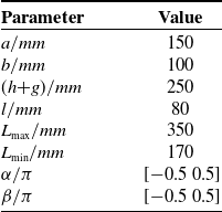
The workspace of a parallel mechanism is a key indicator for performance evaluation. In comparison to series mechanisms, the workspace of parallel mechanisms is constrained by various factors, including the length constraints of the driving branch chains, interference conditions between the branch chains, and limitations on the rotational range of the motion pairs. These constraints are significantly more numerous than those affecting series mechanisms, resulting in a relatively smaller workspace for parallel mechanisms [Reference Yang, Ye and Li32–Reference Hamida, Laribi, Mlika, Romdhane and Zeghloul33]. In this paper, the Monte Carlo method is employed to determine the workspace of the proposed reconfigurable parallel mechanism. Initially, a set of random pose parameters is generated and then substituted into the mathematical model established on the basis of the inverse kinematics equation. By assessing whether the constraint conditions presented in Table II are satisfied, it can be determined whether this set of pose parameters represents an achievable pose of the mechanism. The O1 point on the moving platform is chosen as a reference point, and the pose parameters that meet the constraints are substituted into the coordinate expression of the O1 point to acquire the reachable positions of the moving platform in space. Once a sufficient number of pose points satisfying the constraints are obtained, the workspace of the parallel mechanism can be derived. The relevant constraint parameters are detailed in Table II.
Geometric structure parameters of reconfigurable parallel mechanism.

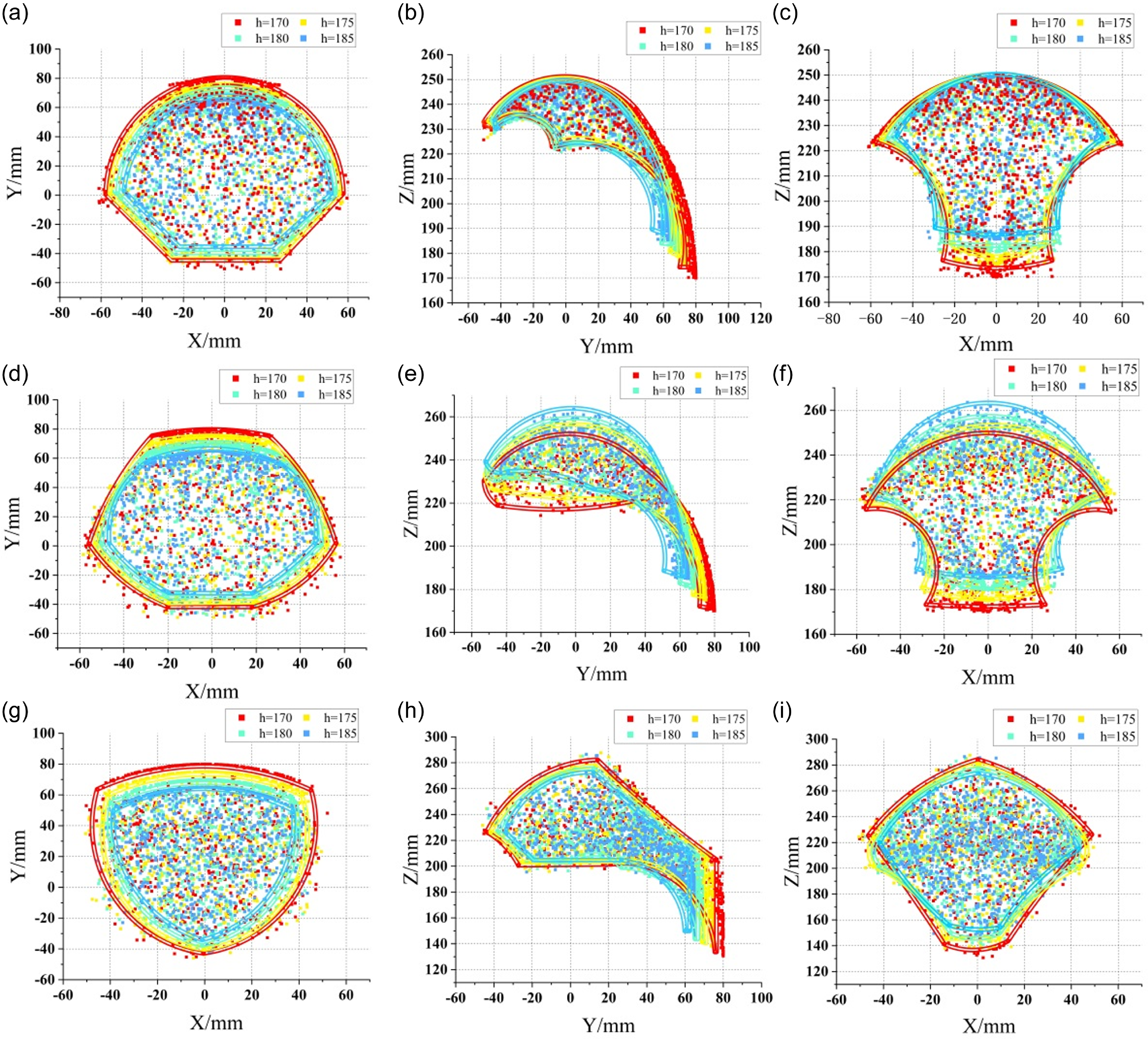
According to the relevant structural parameters in Table II, the three views of the workspace under the three motion modes are obtained, as shown in Figure 7.
Schematic diagram of the relationship between structural parameters and workspace size.

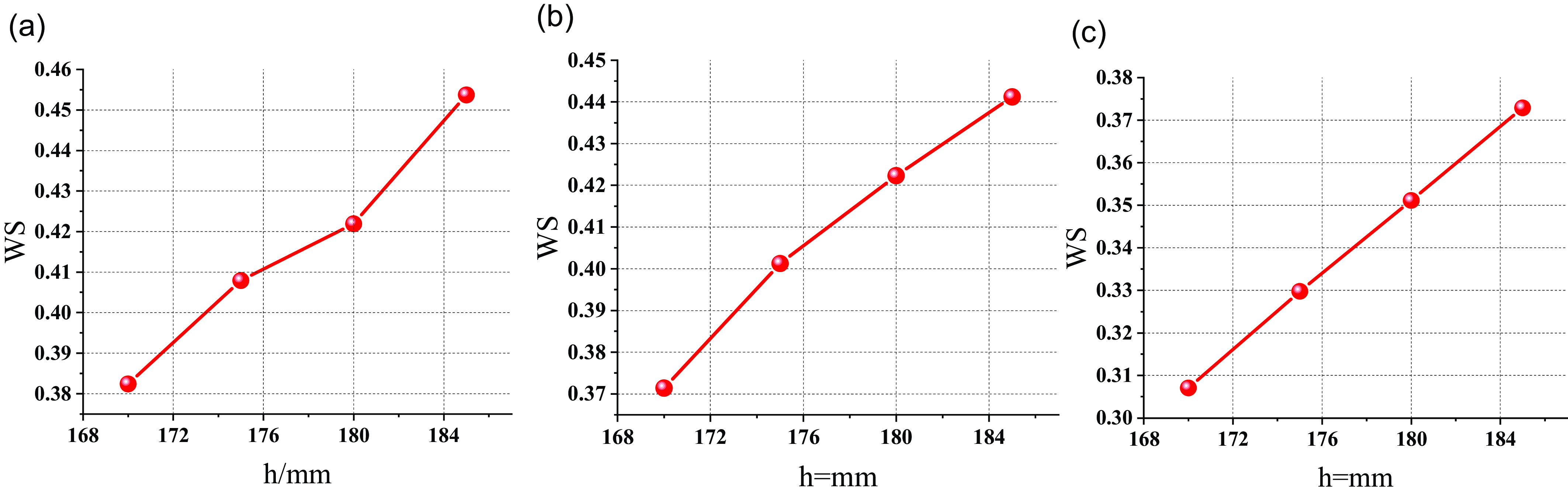
In order to deeply explore the influence of structural parameters on the workspace, based on the characteristics of Monte Carlo method, this study reveals the specific influence of structural parameters h on the workspace size by adjusting the structural parameter h and calculating the workspace size of the parallel mechanism with Eq. (22).
 \begin{equation} WS=\frac{\mathit{n}}{N} \end{equation}
In Eq. (22), N is the number of initial point clusters, and n is the number of points that meet the constraints.
As depicted in Figure 8, across the three motion modes, the workspaces display a notable degree of similarity and exhibit symmetry characteristics. These are closely linked to the structural symmetry of the parallel mechanism. Additionally, Figure 7 illustrates the relationship between the structural parameter h and the workspace size in the three motion modes. The results reveal that in all modes, the workspace has a tendency to expand with the increase of h.
Workspace 2R mode: (a)–(c); 2R* mode: (d)–(f); 2R1T mode: (g)–(i);.

4.2 Analysis of singular position
Singular poses of parallel mechanisms are critical issues that must be avoided during the design process, as these poses can lead to significant alterations in various properties of parallel mechanisms and may even render the mechanism incapable of movement [Reference Wu and Bai34]. Consequently, a thorough analysis of the singular poses of parallel mechanisms is essential. Through the investigation of the proposed parallel mechanism, two distinct types of singular poses have been identified, as illustrated in Figure 9.
Singular position schematic.

The Jacobian matrix characterizes the velocity–mapping relationship between the joint space and the operational space. When the parallel mechanism assumes a singular pose, the determinant value of the Jacobian matrix becomes singular. Thus, the singular pose of the parallel mechanism can be determined by calculating the determinant value of the Jacobian matrix.
 \begin{equation} K=\left\| J^{\mathit{f}}\right\| \end{equation}
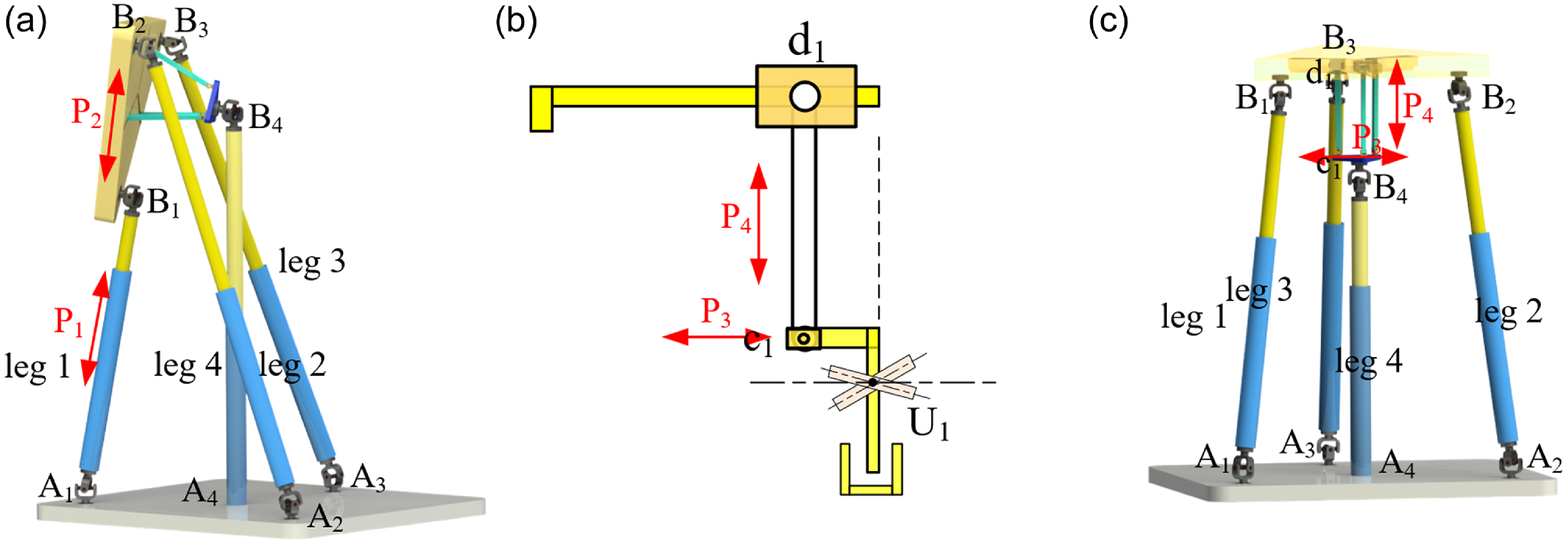
According to Eq. (23) and the structural parameters in Table II, the singular pose of a parallel mechanism designed in this paper can be found out and shown in Figure 9(a). At this time, the vector P1 of the branch chain is parallel to the vector P2 of the moving platform, which is the same as the result obtained in reference [Reference Zhao, Song, Chen, Chen and Ding35]. It is worth noting that the special structure proposed in this paper is not considered when solving the singular pose of parallel mechanism by Jacobian matrix. Through the analysis of the special mechanism proposed in this paper, as shown in Figure 9(b), another singular pose is found, as shown in Figure 9(c). At this time, the L-bar vector P4 in the special structure is perpendicular to the vector P3, which usually occurs in the 2R* motion mode, and will also cause the parallel mechanism to stick and limit its freedom of movement in the Z-axis direction. Therefore, in the actual path planning, these positions should be avoided.
4.3. Dexterity and carrying capacity analysis
The Jacobian matrix reveals the relationship between the moving platform’s output velocity and the actuation joint’s input velocity. Before using the Jacobian matrix to calculate performance indicators, the problems of inconsistent parameter units and varying matrix dimensions must be addressed. Usually, preprocessing the matrix is necessary. A common way to handle unit inconsistency is to normalize the Jacobian matrix by dividing it by the characteristic length. The issue of dimensional inconsistency can be resolved with linear algebra principles. This paper uses this method to deal with Jacobs matrix.
The dexterity index of a parallel mechanism is often represented by the condition number of the Jacobian matrix. The condition number serves as a metric that reflects the accuracy of the matrix, with its value always being greater than or equal to 1. A high condition number indicates a significant distortion in the transfer relationship between the mechanism’s input and output, a situation that designers aim to avoid during the design process. Consequently, the condition number of the Jacobian matrix is extensively employed to assess the dexterity of parallel mechanisms [Reference Merlet36]. The specific calculation equation is as follows:
 \begin{equation} K_{\mathit{j}}=\frac{\sigma _{\max }(J_{\mathit{f}})}{\sigma _{\min }(J_{\mathit{f}})} \end{equation}
In Eq. (24),
 $K_{\mathit{j}}$
represents the condition number of the Jacobian matrix, and
 $\sigma _{\max }\mathrm{,}\sigma _{\min }$
represents the maximum and minimum singular values of the Jacobian matrix. In practical applications, dexterity is often represented by
 $1/K_{\mathit{j}}$
. When the value of
 $1/K_{\mathit{j}}$
is closer to 1, it indicates that the motion transmission performance is better. When the value of
 $1/K_{\mathit{j}}$
is infinite, the mechanism is in the singular configuration.
Notably, the Jacobian matrix of the parallel mechanism is not a constant matrix. Instead, its condition number changes in accordance with the alterations in the pose parameters of the moving platform. This indicates that the Jacobian matrix varies across different poses. As a result, it is inadequate to evaluate the dexterity of a parallel mechanism with a single quantity. To tackle this issue, the global condition index (GCI) proposed by Gosselin is utilized to assess the dexterity of parallel mechanisms.
 \begin{equation} \eta _{J}=\frac{\int _{W}\frac{1}{K_{\mathit{j}}}\mathit{d}_{\mathit{w}}}{\int _{\mathit{w}}\mathit{d}_{\mathit{w}}} \end{equation}
In Eq. (25),
 $\eta _{\mathit{j}}$
is the GCI of the parallel mechanism, and W is the accessible workspace of the parallel mechanism. According to Eq. (25), when the value of
 $\eta _{\mathit{j}}$
is closer to 1, the overall dexterity of the parallel mechanism is higher.
In the kinematic analysis of the mechanism, it can be seen that there is a dual relationship between the velocity Jacobian matrix of the mechanism and the force Jacobian matrix of the mechanism [Reference Zeng, Huang and W.J.37], as shown in Eq. (26):
 \begin{equation} \begin{array}{l} F=Gf\\ G=J_{f}^{T} \end{array} \end{equation}
In Eq. (26),
 $G$
is the Jacobian matrix,
 $F$
is the output force, and
 $f$
is the generalized input force.
The Lagrange equation can be constructed from Eq. (26):
 \begin{equation} L_{F}=f^{T}G^{T}Gf-\lambda _{f}\left(f^{T}f-1\right) \end{equation}
By analyzing Eq. (27), it can be seen that when
 $\| f\|$
= 1, the extreme value of the bearing capacity is the root of the maximum and minimum value of matrix
 $G^{T}G$
, which is defined as the load-bearing capacity performance index:
 \begin{equation} \begin{array}{l} \left\| F_{\max }\right\| =\sqrt{\lambda _{F\max }\left(G^{T}G\right)}=\sigma _{F\max }\left(J_{f}^{-1}\right)\\ \left\| F_{\min }\right\| =\sqrt{\lambda _{F\min }\left(G^{T}G\right)}=\sigma _{Fmon}\left(J_{f}^{-1}\right) \end{array} \end{equation}
Similar to the dexterity index, the load-bearing capacity index calculated by Eq. (28) can only reflect that of a certain pose and is incapable of evaluating the load-bearing capacity of the entire parallel mechanism. To address this, the global load-bearing capacity performance index is employed to assess the load-bearing capacity index of the parallel mechanism within the entire workspace. The calculation formula is presented as Eq. (29).
 \begin{equation} \begin{array}{l} \delta _{{F_{\max }}}=\frac{\int _{\mathit{w}}\left\| F_{\max }\right\| \mathit{dw}}{\int _{\mathit{w}}\mathit{dw}}\\ \delta _{{F_{\min }}}=\frac{\int _{\mathit{w}}\left\| F_{\min }\right\| \mathit{dw}}{\int _{\mathit{w}}\mathit{dw}} \end{array} \end{equation}
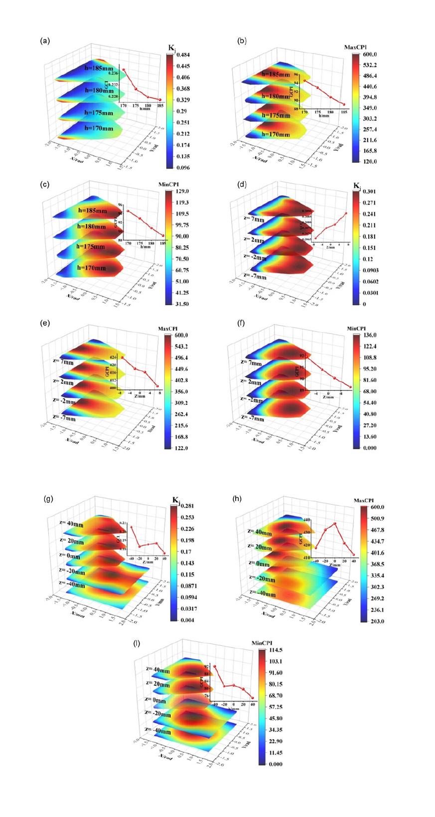
The distributions of the dexterity index and the load-bearing capacity performance index are shown in Figure 10. In each figure, there are schematic diagrams of the global performance indices corresponding to different structural parameters.
As illustrated in Figure 10, the reconfigurable parallel mechanism put forward in this paper showcases outstanding performance in terms of dexterity and capacity performance index. The performance varies in a uniformly transitional manner, thus demonstrating excellent application potential. Significantly, in the 2R mode, alterations in structural parameters have a relatively negligible impact on the performance of the parallel mechanism. This phenomenon verifies that the reconfigurable parallel mechanism proposed herein can achieve a variable rotation center while maintaining favorable performance.
Distribution diagram of dexterity and carrying capacity index 2R mode: (a)–(c); 2R * mode: (d)–(e); 2R1T mode: (g)–(i);.

Similarly, in the 2R* mode, various kinematic performances remain stable. This indicates that, despite having a certain degree of mobility, this mechanism can maintain its performance superiority. Although the fluctuations in global performance indices in the 2R1T mode are somewhat more prominent compared to those in the 2R mode and 2R* mode, it is clear from Figure 10(g)–(i) that the performance indices in the 2R1T mode still display excellent performance. Moreover, the workspace in this mode is even more extensive.
5. Prototype construction
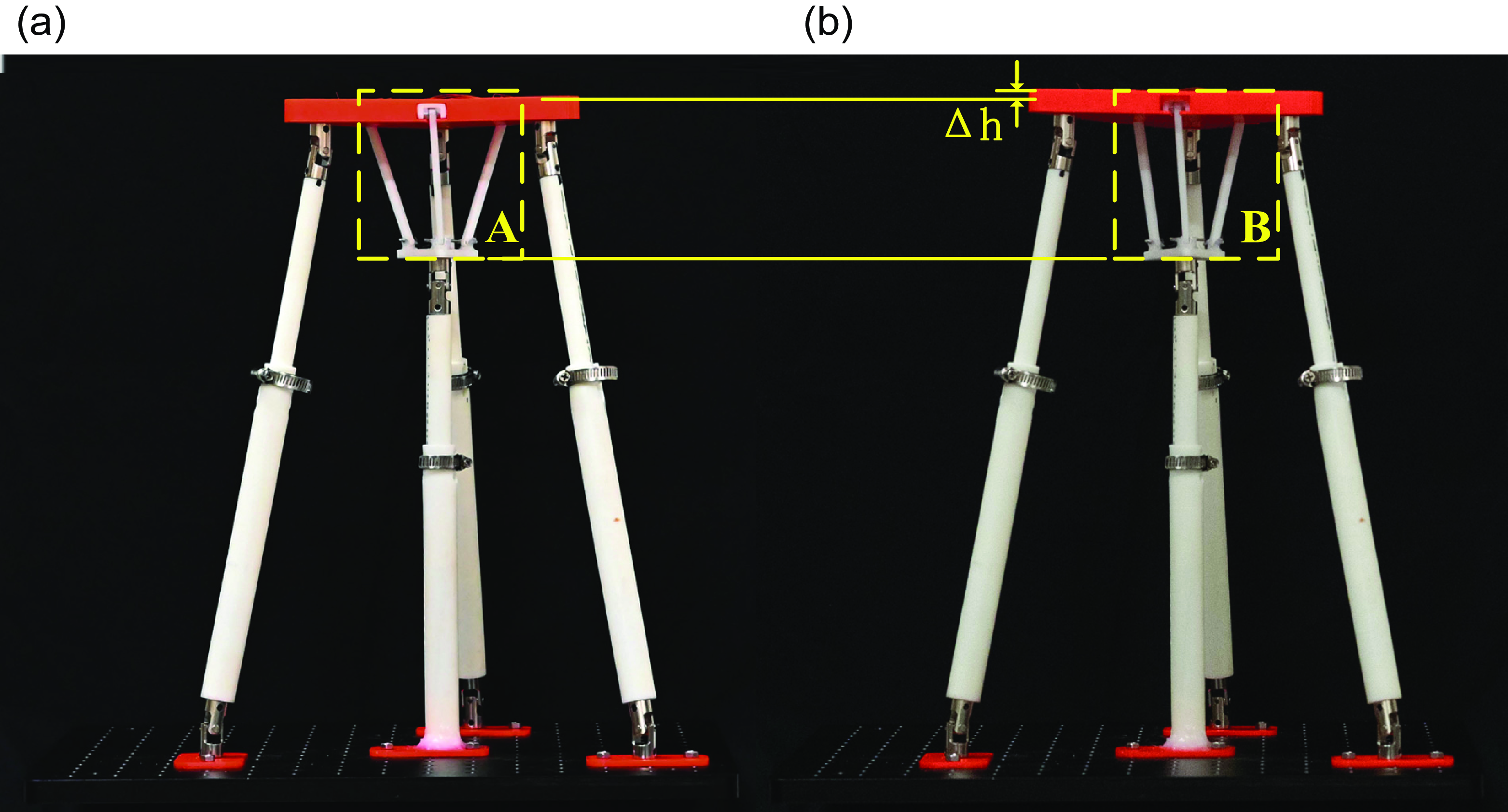
To validate the effectiveness of the specially designed structure in this paper, in this section, based on the structural model described previously, an experimental prototype was constructed using 3D printing technology, with a common prismatic joint replacing the driving limb. Figure 11 presents the constructed experimental prototype, where region A in Figure 11(a) and region B in Figure 11(b), respectively, show the special structure designed in this paper. By comparing Figure 11(a) and (b), it can be observed that adjusting the position of the slider on the moving platform within the special structure can effectively modify the position of the moving platform; while altering the position of the key limb within the special limb, the moving platform remains stable. This phenomenon, to a certain extent, verifies the feasibility of the 2R mode and 2R* mode.
Schematic diagram of prototype construction.

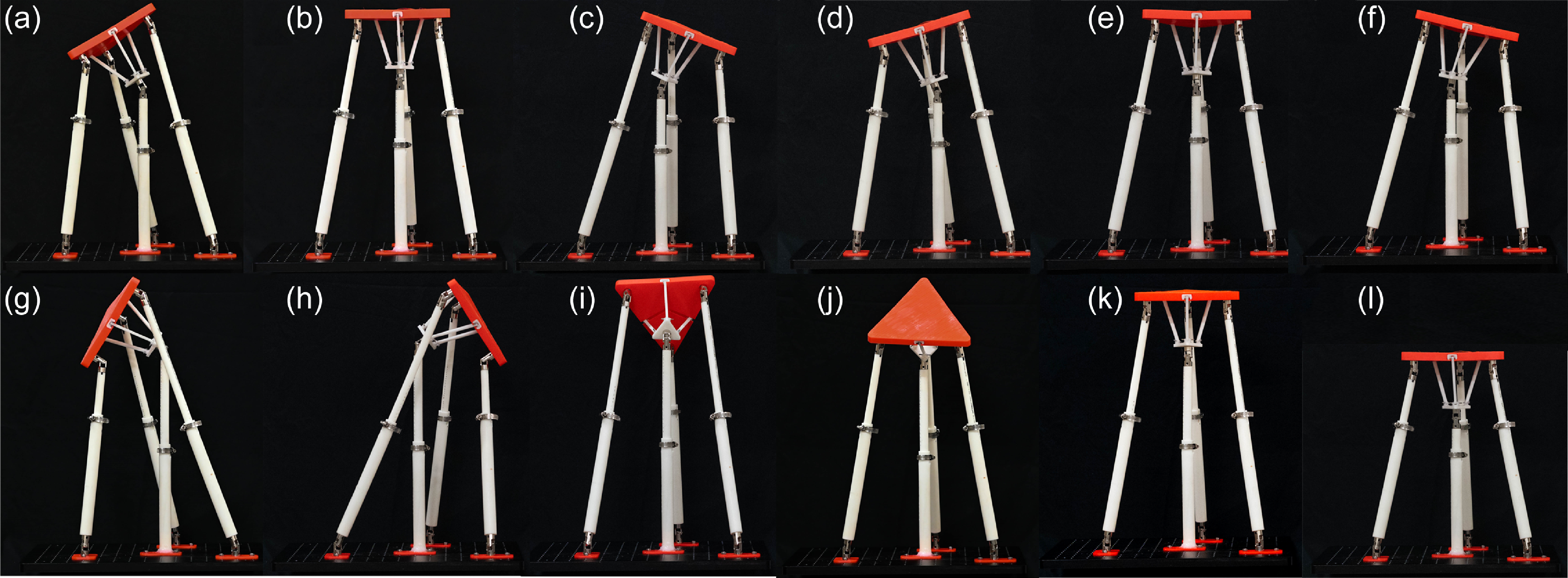
Figure 12(a)–(c) and (d)–(e) are schematic diagrams for validating the 2R mode under different numerical values of the structural parameter h, respectively. Through comparison, it is found that with the variation of the structural parameter h, the special structure can still function effectively. This demonstrates the effectiveness and non-singularity of the special structure designed in this paper, which is applicable to different structural parameters, providing experimental verification for its subsequent application to other parallel mechanisms. Figure 12(g)–(l) shows the schematic diagrams of the extreme poses of the reconfigurable parallel mechanism proposed in this paper. Among them, (g)–(j) corresponds to the extreme poses of the two rotational DOFs and (k) and (l) correspond to the extreme poses of the translational degree of freedom along the Z-axis.
Schematic diagram of degree of freedom verification and limit position under different structural parameters.

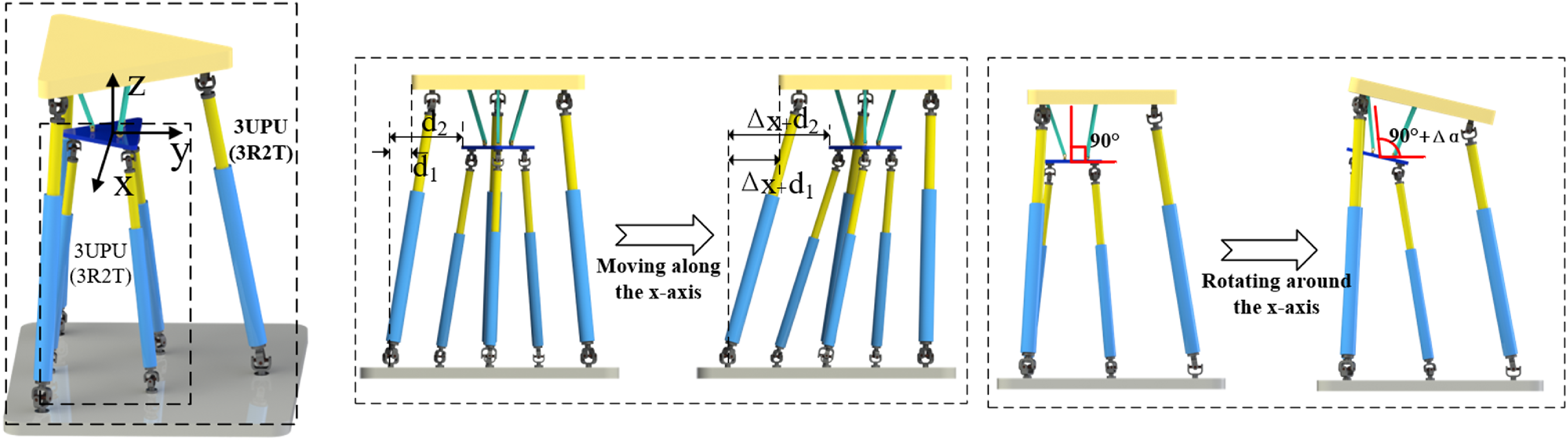
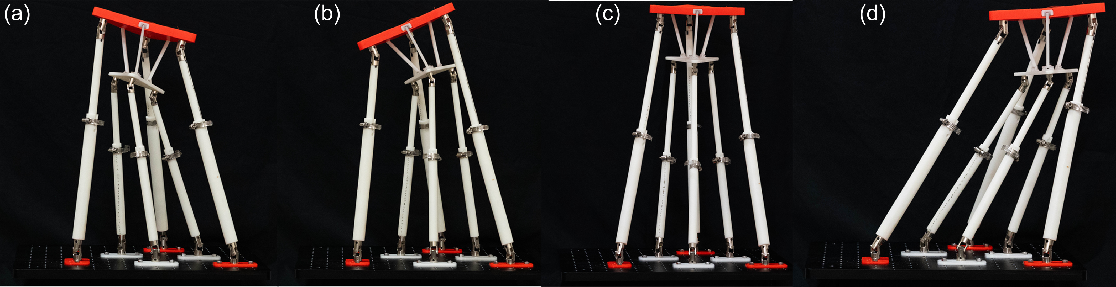
To further verify the effectiveness and universality of the special structure proposed in this paper, based on the prototype in Figure 12, we replaced the key driving branch in Figure 3 with a 3UPU parallel mechanism. The limb arrangement of this 3UPU parallel mechanism is identical to that in Figure 4(a) as demonstrated in Figs. 13 and 14.
2-3UPU reconfigurable parallel mechanism.

Schematic diagram of prototype of 2-3UPU reconfigurable parallel mechanism.

6. Conclusion
(1) Based on a double-slider mechanism, a special structure was proposed. Through the analysis of this special structure, it was found that it exhibits three motion modes. Subsequently, it was applied to the design of a parallel mechanism, endowing the parallel mechanism with reconfigurability and enabling it to switch among three different motion modes. (2) The kinematic analysis of the proposed reconfigurable parallel mechanism was carried out. The inverse kinematic solutions and partial forward kinematic solutions of the three motion modes were, respectively, derived using the vector method and the genetic algorithm. Moreover, the velocity Jacobian matrices in the three motion modes were analyzed by differential method. (3) In-depth analyses were conducted on performance indices such as the workspace, singular poses, and dexterity in the three motion modes. It was discovered that, within the same mode, different structural parameters have a relatively minor impact on various performance indices, suggesting that the proposed reconfigurable parallel mechanism can be more widely applicable to different application scenarios. (4) Based on the designed reconfigurable parallel mechanism, an experimental prototype was constructed to verify the effectiveness of the proposed special structure. Additionally, on the basis of applying the special limb to the parallel mechanism, further expansion was carried out by replacing the driving limb with a parallel mechanism. It was found that the special structure could still function effectively, and by combining the two parallel mechanisms, the parallel mechanism was enabled to acquire reconfigurable characteristics.
Author contribution
Shiqing Lu and Hui Jin contributed to the study conception and design. The first draft of the manuscript was written by Yiqing Xie and all authors commented on previous versions of the manuscript. Data collection and analysis were performed by Weiqiang Lyu and Xia Huang. Review, editing, and validation were performed by Jun Ding. All authors read and approved the final manuscript.
Financial support
This work was supported by Natural Science Foundation of Chongqing Municipality (CSTB2024NSCQ-MSX0143), Science and Technology Research Youth Project of Chongqing Municipal Education Commission (No. KJQN202301104), Cooperative Project between universities in Chongqing and affiliated institutes of Chinese Academy of Sciences (No. HZ2021011), and Unveiling and Challenge-Based Project of Chongqing Yongchuan (No.2024yc-jb gs20001).
Competing interest
The author(s) declared no potential conflicts of interest with respect to the research, authorship, and/or publication of this article