

I. INTRODUCTION
Energy harvesting has been recently demonstrated for various wireless sensor applications, ranging from sensors for health monitoring of patients [Reference Teo, Lim, Sutomo, Tan, Gopalakrishnan and Singh1–Reference Yakovlev, Kim and Poon3], civil engineering structures [Reference Bernhard, Hietpas, George, Kuchima and Reis4], aircraft structural monitoring [Reference Zhao5], sensors in hazardous environments [Reference Cho, Lee, Kong and Chandrakasan6], sensors for covert operations, etc. Typical requirements for such sensors and sensor networks are small size, low maintenance, low available power levels, unknown exact location, and/or maintenance difficulties [Reference Min7]. In these applications, energy is harvested through vibration [Reference Aktakka, Peterson and Najafi8], light, radio frequency (RF) fields [Reference Dolgov, Zane and Popovic9, Reference Vias, Nishimoto, Tentzeris, Hawahara and Asami10], or thermal difference [Reference Doms, Merken, Mertens and Van Hoof11].
A number of researchers have published data for available power densities in the radio frequency spectrum in urban areas in Europe, the USA, and Japan [Reference Vias, Nishimoto, Tentzeris, Kawahara and Asami12, Reference Piñuela, Mitcheson and Lucyszyn13]. The measured power densities at arbitrary locations relative to the transmitters are in the range of 0.1–10 µW/cm2 in the UHF and various ISM. Near or on a base-station tower, harvesting of power from antenna side lobes or reflected power from ground was shown to be sufficient to enable monitoring the base-station activity [Reference Le, Mayaram and Fiez14]. Multiple studies [Reference Haumann, Munzenberg, Maes and Sierck15, Reference Willkomm, Machiraju, Bolot and Wolisz16] have shown that power densities within 50 m of a cell tower exceed 1 µW/cm2 but vary widely with location and time of day, and are also different for different types of base stations. Research continues on methods for achieving start-up and operation using energy rectified from these RF sources [Reference Prete, Costanzo, Masotti and Romani17]. The low-power levels make it difficult to efficiently harvest the power, since the resulting voltages are below 1 V and require boosting in order to operate standard electronic devices. Owing to the physical limitations of flash and FRAM memory technologies, programmable micro-controller unit (MCUs) generally require a minimum of 1.8 V to operate; a level not available directly from most harvested sources. Other ICs (RF transmitters, op-amps, data converters, etc.) that a harvesting sensor might be constructed from also require similar bias.
A high-level block diagram of a harvesting platform is shown in Fig. 1. Most energy-harvesting devices demonstrated to date require either continuous powering or a pre-charged storage element that should never be fully discharged, whether it is capacitor or a chemical cell [Reference Doms, Merken, Mertens and Van Hoof11]. However, this is a special case; in general, it must be assumed that the storage element may become depleted, and some method is required to initially start up the system.
Block diagram of a wireless device that obtains energy by harvesting vibration, light, radio-frequency waves, heat, etc. Low-voltage power conversion and reset circuits are needed to start-up from a depleted state. The MCU controls the power conversion stage and applies MPPT algorithms in addition to collecting and sending data. This paper addresses the shaded elements of the sensor block diagram.

To reliably start-up from a depleted state requires a certain minimum amount of DC power from the harvested source, as well as: (1) boosting the typically very low output voltage available to a value that can be consumed by typical electronics, (2) applying a sharp reset of the resident microprocessor to mitigate the effects of slow V DD supply slew rates; and (3) minimizing overall power consumption to conserve as much energy for the intended application as possible.
Several researchers have investigated fully custom ICs to address these problems [Reference Paing, Shin, Zane and Popovic18, Reference Costanzo, Prete, Dini, Filippi, Tartagni and Masotti19]. Rather than focus on a custom approach, this paper discusses the general problems of low-power, low-voltage energy conversion while using commercially available electronic components. Specific circuits for start-up and reset from a state with no stored energy are presented. It is assumed that bulk capacitance is used as the energy storage element.
II. LOW-VOLTAGE POWER CONVERSION
The voltage available from a harvested source is typically low, <1 V. A power conversion stage is necessary to convert the available power to a higher voltage suitable for consumption by typical electronics.
A) Low-voltage conversion circuits
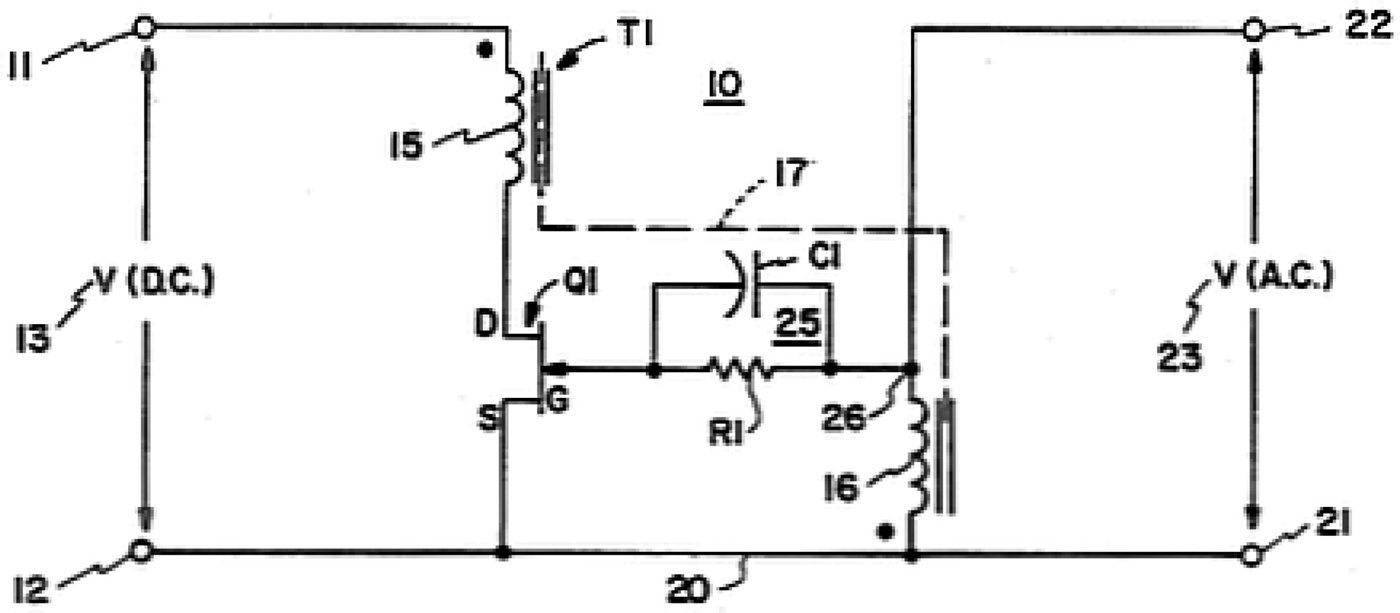
Energy harvesting has been done for quite some time. In 1988, Honeywell patented [Reference Bohan20] a self-driven oscillator (Fig. 2) intended to boost the output of a thermo electric generator (TEG) driven by a pilot flame having an output voltage less than 100 mV, to a level compatible with CMOS digital circuitry. There has been renewed interested in this circuit [Reference Grgic, Ungan, Kostic and Reindl21] with demonstrated startup from V IN = 6 mV, although rather extraordinary lengths were taken to achieve enough feedback gain to ensure oscillation, and a secondary capacitive voltage-doubling stage was employed to further increase the DC output voltage.
US Patent 4734658, circa 1988; [20] oscillator based on a depletion mode JFET, Q 1, that converts very low voltage DC (13), less than 100 mV, to a much higher peak AC voltage (23) that may later be rectified back to DC. The input impedance of this circuit may be too low for some harvesting applications.
This type of conversion circuit employs a depletion mode amplifier in a variation of the Hartley oscillator to transform a low-voltage DC source to a much higher peak voltage AC waveform that is later rectified. The turns-ratio of the transformer, T 1, may be 1:100 or higher.
Commercially available surface mount transformers support this application [22], as well as ICs [23], and even whole converter modules [24]. The primary drawback of this approach is its very low and uncontrollable input impedance. The output impedance of many harvesting sources is too high to effectively couple into this converter, especially under startup conditions. The inability to control the input impedance also makes it impossible to apply a maximum power point tracking (MPPT) algorithm. Nevertheless, this sort of approach is the only viable solution for very low available voltages, <300 mV, where there is not enough bias to startup using enhancement-mode devices.
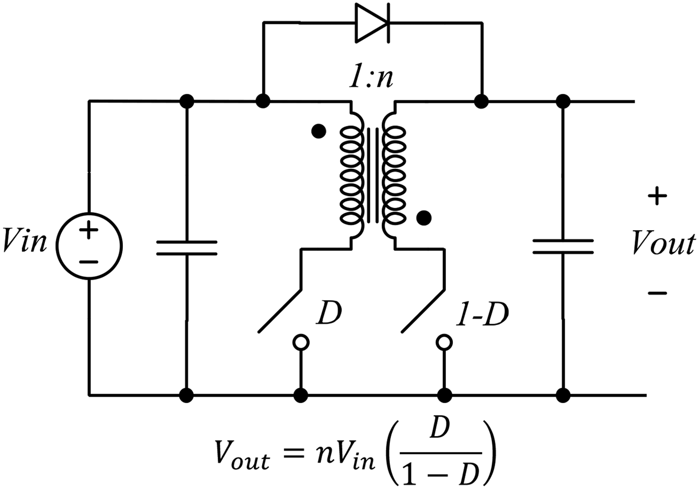
The Flyback and Boost topologies may be used where enough native bias is available to power a local bootstrap oscillator and switching transistor, >300 mV. In energy-harvesting applications these converters usually operate in discontinuous conduction mode (DCM) due to the relatively small switching currents involved. In DCM, the current in the inductor/transformer returns to zero during each switching cycle and the average current into the power converter may be modulated by changing the pulse-width modulator (PWM) timing parameters, D, of the main switching element. This effectively emulates a resistor [Reference Paing, Shin, Zane and Popovic25] and the converter's input impedance, Z in = V in/I in, may be dynamically controlled to match the maximum operating point of the harvesting source if desired.
Should the current increase and the converter enter continuous conduction mode (CCM), volt–second balance on the inductor or transformer will determine the operating voltages of the converter and the input current can no longer be inferred from the PWM timing parameters. In CCM, some direct method of measuring either the input or output current is required to determine the converter's operating point and if power transfer is increasing or decreasing.
The Flyback circuit of Fig. 3 can easily incorporate efficient synchronous rectification since both switching elements are on the low side. The diode coupling the input to the output allows startup current to flow and energize a low-voltage bootstrap oscillator to initiate voltage conversion. The turns-ratio of the transformer should be chosen for reliable startup at the minimum acceptable power.
Flyback converter with duty cycle D having a turns-ratio n and a diode from primary to secondary to allow startup current to flow. Equation valid only for CCM. In DCM mode V out will be load dependent and less than the CCM case. Small, commercially available surface-mount transformers supporting this circuit are available [22].
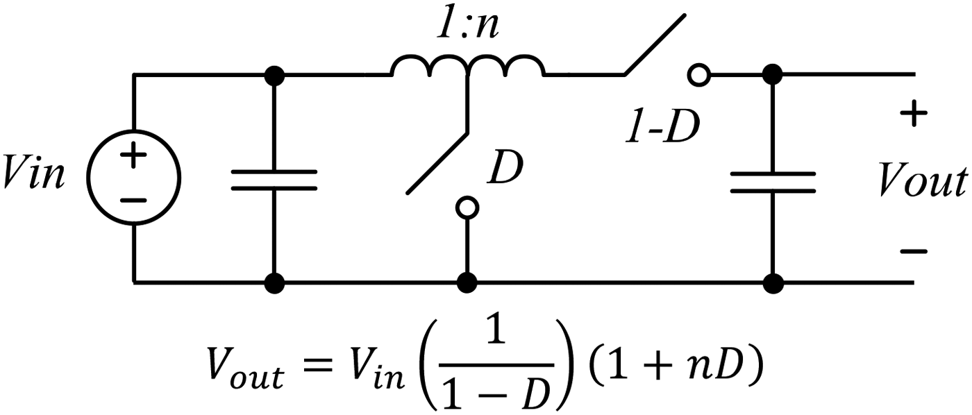
The boost converter of Fig. 4 is commonly used, often in the inductor special case, n = 0. For example, an extremely low-power custom IC [Reference Paing, Shin, Zane and Popovic18] as well as a commercial device [26] is based on this topology operating in DCM. The factor of 1/(1−D) in both the Flyback and Boost topologies can lead to difficulty in controlling power conversion at high boost ratios where the duty cycle D → 1. Circuit losses limit the maximum achievable voltage boost ratio (typically D max ≈ 80%), and control may be difficult if digitally synthesized PWM is employed unless very fine PWM resolution is available. To achieve a lower duty cycle (D ≈ 0.5) that is easier to control for a given V in an V out, the turns-ratio, n, may be chosen to satisfy circuit operation
Boost converter. The special case n = 0 (inductor) is very common. The equation shown is valid for CCM mode. In DCM mode V out will be load dependent and less than the CCM case. Commercially available surface mount 1:1 dual-wound inductors such as [27] may be used for the case n = 1. A variety of other turns ratios may be obtained using modular magnetics such as [28].
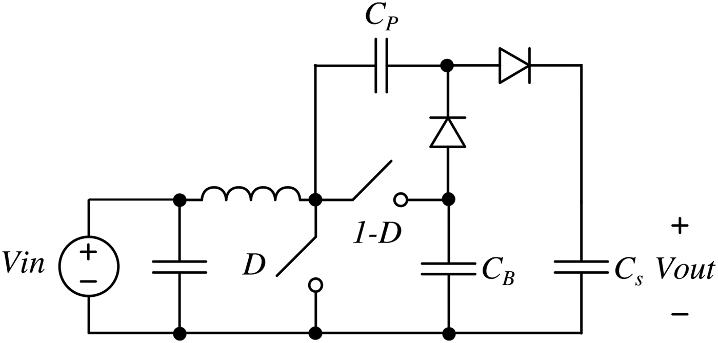
The use of transformers may be undesirable or limited for a variety of reasons. If insufficient voltage is obtained from a given circuit, an additional capacitive voltage multiplier may be added to further boost potential, as was shown in [Reference Grgic, Ungan, Kostic and Reindl21]. For instance, a voltage-doubling stage is added to the boost converter in Fig. 5 operating with duty cycle D. The pump capacitor C P is much smaller than the boot capacitor C B and the bulk capacitance C S attaches to the output of the doubling stage.
Boost converter (n = 0) with added capacitive voltage doubling stage to further increase output voltage. C P ≪ C B, and storage capacitance C S of the sensor is located at the output, V out.
As the boot capacitor charges up, charge is transferred from the boot capacitor, C B, to the pump capacitor when the switch, D, is closed. The inductor is also magnetized during this portion of the switching cycle. When D is opened and (1−D) closed, energy is transferred from the inductor to the output through the pump capacitor and also recharges the boot capacitor. Such voltage multiplier circuits can be added to most every circuit where a square switching waveform is available, and they can be configured to invert the voltage or be cascaded for additional voltage boost.
B) Example MCU controlled converter
An example of an MCU-controlled harvester platform based on the boost converter (n = 0) capable of MCU-controlled MPPT is shown in Fig. 6. Initially assume that the storage element C S is discharged. When power is applied to the input, due to the exponential nature of D 1 current I I flows through L 1, D 1 and V DD gradually charge up. This particular bootstrap oscillator begins operating when V DD ≈ 0.8 V, and drives Q 1 with ~50% duty cycle. The boost stage (L 1, Q 1, D 1) now operates with an unregulated duty cycle and V DD continues to ramp up until reaching 1.8 V, the minimum required for the MCU operation.
(a) Detailed block diagram of an MCU-based energy scavenging controller employing digital PWM control of a boost converter (n = 0); and (b) photograph of implemented start-up circuit.
The 1.8 V regulator [29] power good detector (PG, Fig. 6(a)) then releases the MCU reset pin and code execution begins. The MCU boot code configures its internal clock and PWM timer to generate a digital PWM signal. It disables the bootstrap oscillator and the digital PWM signal is routed through the multiplexer to the gate of Q 1, allowing the MCU to directly control the boost stage.
The voltage and current present at the input of the circuit, V I and I I, is measured using an analog multiplexer and a 12-bit data converter [30] using the 1.8-V regulator output as its power supply and reference. The input current I I is inferred by sensing the DC voltage drop across the switching inductor, L 1. This DC voltage is present due to the non-zero resistance of the inductor, R ESR in Fig. 6. A low-pass network formed by R F, C F removes the switching waveform so that the data converter may digitize V C.
Two data conversions measure V C and V I, and I I∝(V I − V C). The accuracy of this current measurement is poor. However, for the purpose of MPPT it is only necessary to maximize the product V I·I I. This does not require accuracy for either parameter so long as the signals representing V I, I I are proportional to them. For either DCM or CCM operation, the DC input power to the converter is,
 $$P_I = V_I \cdot I_I = V_I \displaystyle{{V_{L_1 } } \over {R_{ESR} }} \propto V_I \lpar V_I - V_C \rpar .$$
Periodically the MCU samples V I, V C and applies the programmed MPPT algorithm to update the duty cycle of the boost stage. When not executing MPPT code or application code, the MCU remains in a sleep state to minimize power consumption. Specifically for this implementation of the MSP430, mode LPM0 is used to halt the processor while maintaining the internal clock to the PWM timer block.
Figure 7 demonstrates the MPPT capabilities of this platform when driven by a resistive voltage source. The source voltage V S and impedance R S are varied, and the regulator executes a “hill climbing” MPPT algorithm to continuously track the maximum power point. For a resistive source, maximum power transfer occurs when V I = 0.5·V S.
(a) Resistive test circuit to measure MPPT tracking versus R s. A 2.5 V shunt regulator absorbs power from power conversion stage. (b) MPPT performance indicates V I closely regulated to 0.5·V S as expected for the resistive source impedance, R S.
Another example of an all-digital MCU-based harvesting platform implementing a synchronous boost converter operating in DCM mode is found in [Reference Dolgov, Zane and Popovic31]. In this case fully synchronous rectification in used, but no start-up oscillator is included; a local battery is assumed to be present.
III. RESET/SUPERVISOR CIRCUITS
Referring back to Fig. 1, due to the low-power levels involved and assuming a relatively large storage capacitance, the slew rate of the MCU power supply, V DD, may be extremely slow, <0.1 V/s or slower. A simple RC network attached to the reset pin of the MCU (often seen in data sheets) intended to provide a delayed rising edge of the reset pin will simply track the slowly rising V DD. Even if the chosen MCU contains an on-board low-voltage detection and/or reset circuit, it may still fail to properly start under these conditions. Should difficulty be encountered in this regard, there are a variety of external reset strategies that can be applied.
As seen in [23, 26, 29] many commercially available power conversion devices intended for very low power or harvesting applications include an open-drain “Power Good” output having a pull-up resistor to V DD. This output may be tied directly to the reset pin of the MCU, and is released when adequate bias is available to reliably operate the MCU. There are also discrete supervisor circuits that require very low bias currents, <150 nA, to properly operate such as [32].
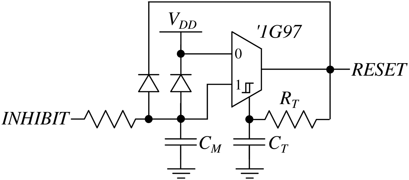
Alternatively, a low-frequency (~100 Hz, ~50% duty cycle) relaxation oscillator can apply a series of reset pulses until the MCU properly starts. Once booted and configured, the MCU disables the oscillator to prevent a subsequent reset. Figure 8 shows such an oscillator constructed from a single gate logic device [33]. Once disabled, the quiescent current is reduced to only that of the static logic gate and may be extremely small.
Reset oscillator based on the '1G97 multi-function logic gate configured as a multiplexer. Input hysteresis allows for oscillation frequency f ≈ 1/(R T·C T). Once booted, an MCU GPIO pin asserts INHIBIT high halting the oscillator with RESET in the high state to prevent a subsequent reset.
Suppose RESET is an active-low signal. The diodes discharge the capacitor C M when either V DD or RESET is low. INHIBIT is tied to an MCU GPIO pin that's assumed to be in a high-impedance state when the MCU is in reset. After the MCU properly boots up, it asserts INHIBIT high, charges C M to halt the oscillator, and RESET is left high. A low-power watchdog timer such as [34] may also be a good choice to apply a periodic forced reset signal.
As a side note, rarely do logic gate manufacturers' data sheets specify the typical quiescent current for static operation. It is test-time intensive and therefore costly to measure very small currents in a production environment. Instead, only a maximum is given representing a factory test limit that may be orders of magnitude higher than an actual typical gate.
IV. PACKET ENERGY CONSUMPTION PROFILE
After a successful startup of the sensor, it is imperative to conserve energy and have enough left over to do something useful. Harvesting sensors that transmit wirelessly are typically configured to periodically wake up from a low-current (<3 µA) sleep mode, assemble and transmit a data packet over an RF channel, and then go back to sleep. A sensor where the MCU is playing an active role in managing the power conversion process will also need some time to do so. In order to accurately understand the energy needs of the sensor, the dynamic current draw profile must be characterized.
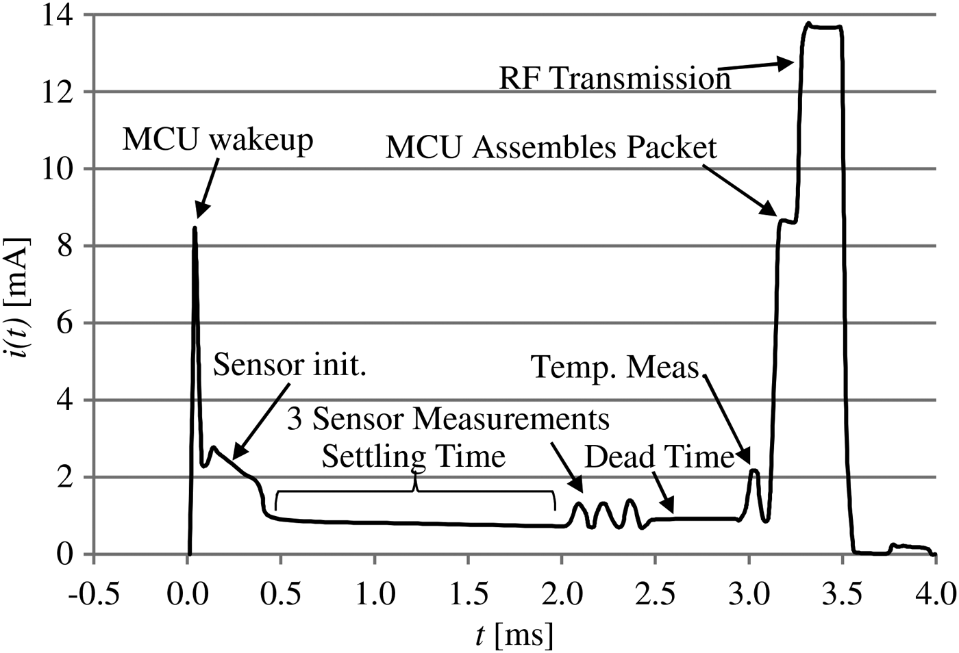
The profile of the current drawn from the storage capacitance during a packet transmission interval of duration T for a typical sensor is shown in Fig. 9. The MCU wakes from the low-current sleep mode and executes several blocks of code to configure the rest of the device for the forthcoming packet transmission. In this case, a sensor that requires about 1.5 ms of settling time is initialized and allowed to settle. After the settling time, three measurements are taken. Following a dead time, a fourth measurement is sampled (temperature). The MCU then assembles the data into a packet, and keys the RF transmitter to transmit it before going back to the sleep state.
An example of dynamic current drawn from the storage element during a packet transmission [35]. Total charge drawn is the area under the curve. Settling and dead times should be minimized or avoided to minimize Q T and packet energy.
The total amount of charge drawn from the on-board storage capacitance is
 $$Q_T = \int_0^T {i\lpar t\rpar dt}\comma \; $$
and the energy consumed during the packet is
 $$E_W = V \cdot Q_T\comma \; $$
where V is the potential of the storage capacitance. The current drawn to operate the various electronics is fixed so the only way to minimize Q T, and therefore E W, is to execute all the elements of the packet as quickly and efficiently as possible; T must be minimized.
Wireless packet transmission usually represents the largest consumption of energy. For a sensor with a periodic packet transmission frequency F, the average current drawn from the bulk capacitance is approximated by
 $$\langle i\rangle = Q_T \cdot F\comma \; $$
and the average power drawn from the storage capacitance is,
 $$\langle P\rangle = V \cdot \langle i\rangle = E_W \cdot F\comma \; $$
assuming V is constant. Clearly (5) shows that power consumption scales linearly with voltage. This implies that for best efficiency, the local storage capacitance should be maintained at the lowest voltage possible to operate the electronics.
This may create a dilemma: the power available from the source is usually variable but if the storage element is somehow kept at a fixed voltage, the power consumed by the sensor is constant when using a fixed transmission period. There will almost always be imbalance between the supply and demand of available power. This issue is accentuated if MPPT is applied, as the dynamic range of available power increases.
If the application can tolerate it, an elegant solution to this problem is to allow the sensor to operate more frequently as more power is available, i.e. increase F [Reference Falkenstein, Costinett, Zane and Popovic36]. This is easily accomplished by simply monitoring the voltage of the storage element and initiating a transmission once a threshold value is exceeded. During transmission, the storage voltage drops below the threshold, and the harvester recharges it in the interim time. If the application demands a fixed transmission rate, energy harvesting must be suspended before the upper damage limit of the storage element is reached.
V. POWER MANAGEMENT, CONTROL, AND MPPT
Contemporary CMOS MCUs designed for low-power operation include a variety of low-power modes intended to conserve power by disabling or configuring the various internal clocks. A major portion of the MCU firmware is devoted to power management, and therefore entry into and exit from the low-power modes.
When not in a low-power mode, the MCU operates in Active Mode where current draw can be substantial, mA of current as shown in Fig. 9, while executing code. The MCU may only operate in this mode for very short bursts, often <1% of the time, to achieve an average power draw low enough to meet the power budget.
The design of the sensor becomes one of evaluating the trade-offs between the available power, the requirements of the application, the power modes available for use, and capabilities of the MCU to move quickly between low-power standby modes and energy intensive computing.
A) MCU standby power management
The two most relevant MCU power saving modes can be categorized as: (1) “hibernate” or “memory retention” where all clocks are stopped and certain internal circuit elements are disabled, and (2) “RTC”, meaning “Real Time Clock”, where only a low frequency oscillator, 5–60 kHz, operates. Often a 32.768 kHz low-power “tuning fork” crystal is used for this mode to provide a convenient and stable time base for time-keeping, although MCUs now exist that have integrated oscillators with similar power consumption but poor timing tolerance [37].
Hibernation mode will always be the most energy efficient and at room temperature, a power savvy MCU can achieve a typical hibernating current of 100 nA. Unfortunately, the only way to revive an MCU from this state is with some sort of external stimulus such as from a sensor or an external timer. A sensor capable of initiating such an event usually consumes far more quiescent power than the dormant MCU, overshadowing it in terms of the energy budget.
The RTC mode is also very efficient, but in this mode the MCU is also capable of waking itself. MCUs with this feature are available that can operate with a 32.768-kHz crystal or integrated low-frequency oscillator, while typically consuming 500–700 nA. The lowest current solution capable of self-wakeup combines the Hibernation mode with a purpose-built external timer, e.g. [34]. This timer is capable of typical operation of 30 nA, allowing a sensor system to lie dormant but wake itself on a combined current of 130 nA.
The previous discussion represents the overhead current consumption simply to maintain the MCU in a known state and perhaps periodically wake itself. All other electronics connected to the on-board storage capacitance will also draw some quiescent current, unless additional transistors or other means to disconnect them are designed to remove the load. Furthermore, no power or application management code is included; once the MCU begins to do something useful in Active mode, power consumption increases dramatically.
B) Active mode current
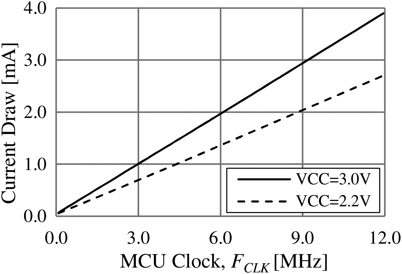
Figure 10 shows the current draw of a power-optimized CMOS MCU while in Active Mode. Current consumption scales linearly with clock frequency and is a function of applied V CC.
Current consumption of a CMOS MCU scales with clock frequency and is also a function of applied voltage. Note that at F CLK = 0 Hz, the current does not become 0.0 mA; I 0 ≠ 0 mA.
The energy required to operate the MCU in this mode for a time T is
 $$\eqalign{E_{MCU}& = V_{CC} \cdot Q_{MCU} \lpar T\rpar \cr& = V_{CC} \int_0^T {[I_0+m\lpar V_{CC} \rpar F_{CLK}]dt} \cr& = \; V_{CC} TI_0 + V_{CC} m\lpar V_{CC} \rpar T\; F_{CLK}\comma \; } $$
where m(V CC) is the linear slope of the current versus clock frequency for a given V CC supply voltage and I 0 represents the non-zero Active mode current when F CLK = 0 Hz. The term V CC·T·I 0 represents an overhead loss that produces no useful result and the latter term represents the energy consumed in computing the task at hand, i.e. see Fig. 9.
Since I 0 is constant, overhead can only be minimized by reducing V CC and T. T is minimized by executing the most efficient code possible since the number of CPU instructions executed is proportional to the product T·F CLK. Furthermore, as evident from Fig. 10, the slope m is smaller for lower values of V CC indicating an additional second-order improvement to power consumption by operating at the lowest possible V CC.
C) Maximum power point tracking
A variety of MPPT algorithms exist and a synopsis of them may be found in [38, pp. 21–35]. The low-power levels and relatively large storage capacitance found in energy harvesters tend to limit the need for high speed, high precision power point tracking. Instead, the basic “Perturb and Observe” (P&O) hill-climbing method is usually sufficient.
In this method, the power conversion stage parameters are constantly varied, but reverse direction when declining power is detected. For example, suppose a boost converter stage is used and the PWM duty cycle is increasing versus time, resulting in an increasing average input current. If this change causes a reduction in power transfer, the duty cycle increment changes from increasing to deceasing, i.e. the scan direction is changed. The duty cycle continues scanning in this direction until power transfer again declines. The main disadvantage to this method is that it is unstable as it constantly hunts for the peak point.
Simpler than P&O is fractional open-circuit voltage (FOCV). This method is not a true “power tracking” algorithm, but instead assumes that the maximum power point will occur close to some known fraction of the source's open-circuit voltage. Periodically the controller halts power transfer and samples the open-circuit voltage. The controller then regulates the input voltage of the power converter to match a programmed fraction of the open-circuit voltage. The ability to track the peak power point is limited by the validity of the fractional voltage assumption, but in many cases still results in relatively good performance. It is very simple to implement, is the method chosen for [Reference Costanzo, Prete, Dini, Filippi, Tartagni and Masotti19, 26], and is well suited to photo-voltaic sources.
VI. WIRELESS DEVICES
A variety of commercially available integrated transmitters, transceivers (TRX) and System-on-Chip (SoC) having an on-board MCU are available that support operation across the spectrum. Commonly used license-free frequencies include 315 MHz, 433 MHz, 868 MHz, 915 MHz, and 2.45 GHz, although only the use of 2.45 GHz is harmonized worldwide.
315 and 433 MHz are commonly used to transmit a control signal, such as a garage door opener, but some data are permitted to be sent along with the control signal [39]. In the USA, frequency hopping and digital spread spectrum techniques allow for transmission powers up to +30 dBm in the 915 MHz and 2.45 GHz ISM bands, otherwise transmit power may be limited to as low as −0.5 dBm [40]. Operating power limits in the 868 MHz band vary greatly depending on the bandwidth and even the intended application per ETSI EN 300-220.
If a standard modulation is desirable, IEEE 802.15.4 g supports operation at both 868/915 MHz and 2.45 GHz ISM bands, but may be overly complex, costly or inefficient in some applications. A propriety modulation and bit rate may be tailored to the application for maximum efficiency and may be ASK, OOK, FM, or a more complex digital format. In harvesting applications generally it is most efficient to only transmit data, but a transceiver may still be necessary to comply with certain regulatory rules. In some spectrum allocations, it is mandatory to “listen-before-talk”, i.e. verify that the RF channel is clear, before transmitting on the channel.
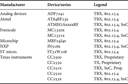
Table 1 contains a sampling of commercially available devices that operate in the 2.45 GHz ISM band. Most devices are transceivers (TRX) and are specifically designed to comply with the IEEE 802.15.4 standard. Some devices are designed strictly for proprietary modulation and bit rates, but some devices that comply with 802.15.4 can support other proprietary modes as well. A device that also contains an embedded MCU is considered an SoC, and a device that is capable of transmit only operation is designated (TX). Operating transmit powers vary from device to device but are generally limited to between 0 and +8 dBm maximum output power.
Commercially available 2.45 GHz wireless devices.
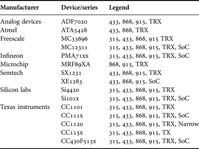
Table 2 contains a sampling of commercially available devices that operate in the ISM and control bands below 1 GHz. The recent revision of IEEE 802.15.4 g defines a variety of modulation modes that may be used in this spectrum, including 50 kbps 2-FSK, which is easily accommodated. Depending on hardware limitations, some devices can only support some of the ISM and control bands below 1 GHz, as shown in the legend. Similar to their 2.45 GHz siblings, TRX, transit-only (TX), and SoC devices exist. Some newer devices such as the CC1120 accommodate very narrow channel spacing down to 12.5 kHz, and have very good sensitivity, −123 dBm at 1.2 kbps, when in receive mode.
Commercially available sub-1 GHz wireless devices.
The native maximum transmit power available from these devices vary more widely, from about +5 to +15 dBm; however, FCC or ETSI rules may limit operation to a lower level depending on the occupied RF bandwidth or application. If this is the case for a particular application then a device with lesser capability may ultimately be more efficient in a harvesting application as the DC power consumption of the TX power amplifier may be lower.
VII. CONCLUSIONS
This paper presents an overview of currently available commercial low-power electronics for energy-harvesting wireless sensors. Although the general low-power electronics is appropriate for harvesting of any type of energy, the focus of the work presented here is on wirelessly powered sensors such as the ones overviewed in [Reference Popovic, Falkenstein, Costinett and Zane41]. In this case, it has been shown that the DC impedance that optimizes power from a rectenna is as high as 100 kΩ for very low-power levels, and typically 10 kΩ down to 300 Ω as the power levels increase. The start-up circuit needs to be matched to an appropriate DC impedance level, which in turn means that a number of obvious circuits will not work efficiently. An approach to solving the start-up problem when the storage element is fully depleted, based on commercially available components is presented.
Although a fully custom power management IC could be used [Reference Paing, Shin, Zane and Popovic18], alternatively the application MCU may digitally control the power conversion stage [Reference Boudreaux, Nelms and Hung42] to optimally charge the energy storage element according to whatever MPPT or other application specific algorithms are desired. This programmable approach may lead to the lowest parts count, smallest size, lowest cost, and potentially best performing solution as every element of the design may be tailored to the specific application at hand, but great care must be given to design and optimization of firmware, both for power management and the application, to ensure an efficient design that overcomes power limitations.
ACKNOWLEDGEMENTS
We would like to thank Sean Korhummel, Research Assistant at the University of Colorado, for helpful discussions and Z. Popovic acknowledges support by the Hudson Moore Jr. Endowed Chair in the College of Engineering and Applied Science. This work was funded in part by a Rehabilitation Engineering Research Center on Advancing Cognitive Technologies, U.S. Department of Education NIDRR (Grant No. H133E040019).
 Steven Dunbar received the BSECE degree from the University of Colorado, Boulder in 1992 and the MSEE degree from the University of Texas, Arlington in 1996. He is now pursuing the Ph.D. at the University of Colorado. He was previously employed by Motorola, Inovonics Wireless Corporation, and RF Micro Devices, and is currently employed at Texas Instruments as a Field Applications Engineer. He is a licensed Professional Engineer (PE) in the State of Colorado, and holds two US Patents.
Zoya Popović received the Dipl. Ing. degree from the University of Belgrade, Serbia, in 1985, and the Ph.D. degree from the California Institute of Technology, in 1990. Since then she has been with the University of Colorado at Boulder, where she is currently a Distinguished Professor and holds the Hudson Moore Jr. Chair in the department of Electrical, Computer and Energy Engineering. Her research interests include high-efficiency, low-noise, and broadband microwave and millimeter-wave circuits, active antennas, applications of microwaves in medicine, and wireless powering for batteryless sensors. She has graduated 50 Ph.D. students, was the recipient of the 1993 and 2006 IEEE MTT-S Microwave Prizes for best journal papers and Distinguished Educator award in 2013. She received the 1996 URSI Issac Koga Gold Medal, a 2000 Humboldt Research Award from the German Alexander von Humboldt Stiftung, and was named an NSF White House Presidential Faculty Fellow in 1993.