1 Introduction
Separated and reattached turbulent flows have received significant research attention prompted by their importance in advancing fundamental understanding of complex turbulent shear flows, and widespread engineering and environmental applications. For instance, a thorough understanding of the unsteady characteristics of separation and reattachment is of great importance for the development of optimal control stratagem for flow-induced structural vibrations, acoustic noise and mitigating structural resonance. An in-depth knowledge of the underlying flow physics is also necessary for reliable prediction of aerodynamic loads on buildings. In the case of low-rise buildings, their heights are typically smaller than the boundary layer thickness (
 $\unicode[STIX]{x1D6FF}$
), and for a building or bluff body immersed in a deep turbulent boundary layer (i.e.
 $\unicode[STIX]{x1D6FF}\gg H$
, where
 $H$
is the height of the bluff body), the characteristics of the approaching boundary layer flow that the bluff body sees include strong mean shear, high turbulence intensity and large-scale streamwise-elongated coherent structures. These characteristics can severely complicate the flow physics, for instance, in comparison to bluff bodies in a uniform oncoming flow, and pose significant challenges to fundamental understanding of the associated separated and reattached turbulent flows. While considerable research has been dedicated to two-dimensional bluff bodies in a uniform flow (Kiya & Sasaki Reference Kiya and Sasaki1983; Cherry, Hillier & Latour Reference Cherry, Hillier and Latour1984), a laminar boundary layer (Stüer, Gyr & Kinzelbach Reference Stüer, Gyr and Kinzelbach1999; Wilhelm, Härtel & Kleiser Reference Wilhelm, Härtel and Kleiser2003; Lanzerstorfer & Kuhlmann Reference Lanzerstorfer and Kuhlmann2012) or thin (compared to the body height) turbulent boundary layers (Djilali & Gartshore Reference Djilali and Gartshore1991), much less has been documented on two-dimensional bluff bodies immersed in a deep turbulent boundary layer. Therefore, the motivation of the present study is to provide a detailed investigation on the interactions of a deep upstream turbulent boundary layer with a two-dimensional surface-mounted bluff body, with particular focus on the unsteady characteristics of turbulent separations and the inherent turbulence structures.
Turbulent boundary layers (TBL) over a forward-facing step (FFS) and a backward-facing step (BFS) are two canonical cases that are routinely used to investigate the characteristics of turbulent separation and reattachment. Many research works were dedicated to the investigation of the effects of the relative step height (
 $\unicode[STIX]{x1D6FF}/H$
), Reynolds number and surface roughness on the reattachment length and one-point statistics including the mean velocities and Reynolds stresses (Piirto et al.
Reference Piirto, Saarenrinne, Eloranta and Karvinen2003; Hattori & Nagano Reference Hattori and Nagano2010; Sherry, Lo Jacono & Sheridan Reference Sherry, Lo Jacono and Sheridan2010; Essel & Tachie Reference Essel and Tachie2015, Reference Essel and Tachie2017). By using a planar particle image velocimetry (PIV), Sherry et al. (Reference Sherry, Lo Jacono and Sheridan2010) measured the turbulent separation bubble (TSB) over an FFS immersed in TBLs with different values of
 $\unicode[STIX]{x1D6FF}/H$
and Reynolds numbers. They observed that for Reynolds numbers (defined based on step height and free-stream velocity) lower than 8500, the reattachment length increases as Reynolds number increases, whereas for Reynolds numbers larger than 8500, the reattachment length does not vary significantly. Essel & Tachie (Reference Essel and Tachie2017) investigated the effects of Reynolds numbers and upstream wall roughness on turbulent flows over an FFS using a planar PIV. For upstream TBLs over smooth walls, the reattachment length of the separation bubble on the FFS increased linearly with Reynolds number up to 6380 beyond which no further change in reattachment length was observed. On the contrary, they observed that the reattachment length for the upstream TBLs over rough walls decreased initially with Reynolds number and attained Reynolds number independence at a Reynolds number of 4000. Hattori & Nagano (Reference Hattori and Nagano2010) performed a direct numerical simulation (DNS) study for TBLs over an FFS. They observed that near the leading edge of the step, Reynolds shear stress (
 $\overline{u^{\prime }v^{\prime }}$
, where
 $\overline{(\cdot )}$
denotes time averaging,
 $(\cdot )^{\prime }$
represents the fluctuating component,
 $u$
and
 $v$
are the streamwise and vertical velocities, respectively) and mean shear (
 $\overline{S}_{12}=(\unicode[STIX]{x2202}\overline{u}/\unicode[STIX]{x2202}y+\unicode[STIX]{x2202}\overline{v}/\unicode[STIX]{x2202}x)/2$
, where
 $x$
and
 $y$
denote the streamwise and vertical directions, respectively) change signs at different locations, which implied the occurrence of negatively valued eddy viscosity and deviation from the conventional Boussinesq eddy-viscosity assumption. By employing a stereo PIV, Piirto et al. (Reference Piirto, Saarenrinne, Eloranta and Karvinen2003) estimated the transport equations of turbulent kinetic energy (TKE) for flows over a BFS. Their results indicated that the dominant budget terms for TKE are the viscous dissipation and production, and their peak locations coincide well at different streamwise locations. With a planar PIV, Essel & Tachie (Reference Essel and Tachie2015) measured turbulent flows over different wall roughness downstream of a BFS and concluded that wall roughness tends to increase the mean reattachment length behind the step.
Considerable research efforts have also been made to understand the unsteady characteristics of turbulent separations. For separation over a blunt body in a uniform oncoming flow, Kiya & Sasaki (Reference Kiya and Sasaki1983) and Cherry et al. (Reference Cherry, Hillier and Latour1984) observed a low-frequency flapping motion associated with enlargement/shrinkage of separation bubbles, and a higher frequency induced by vortex shedding towards the downstream direction. Similar observations were made by Hudy, Naguib & Humphreys (Reference Hudy, Naguib and Humphreys2003) and Mohammed-Taifour & Weiss (Reference Mohammed-Taifour and Weiss2016) for separations induced by a fence and an adverse pressure gradient, respectively. The low-frequency flapping motion has been extensively studied (Eaton & Johnston Reference Eaton, Johnston, Bradbury, Durst, Launder, Schmidt and Whitelaw1982; Driver, Seegmiller & Marvin Reference Driver, Seegmiller and Marvin1987; Simpson Reference Simpson1989; Largeau & Moriniere Reference Largeau and Moriniere2007; Camussi et al. Reference Camussi, Felli, Pereira, Aloisio and Di Marco2008), and is commonly identified as a sharp peak in the frequency spectra of some parameters (such as velocity fluctuations) associated with turbulent separations. Nonetheless, the underlying physical mechanism of the low-frequency flapping motion is still not well understood. Eaton & Johnston (Reference Eaton, Johnston, Bradbury, Durst, Launder, Schmidt and Whitelaw1982) performed measurement in turbulent flow behind a BFS using both hot-wire probes and thermal tuft probes, and observed that a significant fraction of turbulence intensity was contributed by low frequencies. They speculated that the low-frequency flapping motion was caused by the instantaneous imbalance between shear layer entrainment from the recirculating region and reinjection of fluid near the reattachment point. Driver et al. (Reference Driver, Seegmiller and Marvin1987) used a thermal tuft and a laser-Doppler velocimetry (LDV) to simultaneously measure the wall friction and velocity field over a BFS. By employing conditional averaging based on flow direction near the reattachment point, they deduced that the flapping motion was caused by the roll-up and pairing process residing in the free shear layer. Spazzini et al. (Reference Spazzini, Iuso, Onorato, Zurlo and Di Cicca2001) used a surface-mounted double hot-wire probe and a planar PIV to simultaneously measure wall friction and velocity field over a BFS at different Reynolds numbers. They conjectured that the flapping motion of separation behind the BFS is related or dominated by the cyclic behaviour of the recirculation bubble near the leeward corner. Lee & Sung (Reference Lee and Sung2002) employed an acoustical array microphone system and a hot-wire probe to perform simultaneous measurement of the wall pressure and velocity fields in turbulent flows over a BFS. They related the quasi-periodic pressure fluctuation with the flapping motion of the separation bubbles. Camussi et al. (Reference Camussi, Felli, Pereira, Aloisio and Di Marco2008) used surface-mounted piezoresistive pressure transducers and a time-resolved PIV (TR-PIV) system to simultaneously measure the wall pressure fluctuations and turbulent flows over an FFS, and used the cross-correlation of pressure and velocity to reveal the flapping motion. They attributed the flapping motion to the shedding of shear layer structures from the leading edge of the step. Largeau & Moriniere (Reference Largeau and Moriniere2007) observed a similar low frequency as Camussi et al. (Reference Camussi, Felli, Pereira, Aloisio and Di Marco2008) in wall pressure fluctuations, and attributed it to the vortex shedding near the reattachment point. More recently, Pearson, Goulart & Ganapathisubramani (Reference Pearson, Goulart and Ganapathisubramani2013) investigated the turbulent separation in front of an FFS using a planar TR-PIV system. They observed the flapping motion of turbulent separation through the frequency spectrum of areas of instantaneous reverse flow. By using a conditional averaging technique, they showed that sudden enlargement of separations occurred after impingement of upstream low-velocity flows onto the windward face of the step. They also speculated that strong spanwise flows across the step corner was influenced by the upstream coherent structures.
Unlike FFS and BFS, research on turbulent flows over steps with intermediate aspect ratios is rather scarce in existing literature. Bergeles & Athanassiadis (Reference Bergeles and Athanassiadis1983) performed measurement in turbulent flows over surface-mounted steps with different aspect ratios (
 $1\leqslant L/H\leqslant 10$
, where
 $L$
represents the streamwise length of the step) using a hot wire. With their specific thin upstream TBL (
 $\unicode[STIX]{x1D6FF}=0.48H$
) and low turbulence intensity (
 $0.5\,\%$
), they observed reattachment on the top surface of the step only when
 $L/H\geqslant 5$
, and for these cases, the reattachment length behind the step was not affected by aspect ratio. In other words, for cases with two distinct separation bubbles over and behind the step, interaction between these different mean separation bubbles was negligible. The current paper revisits this observation in a deep TBL with characteristic high levels of turbulence intensity for an intermediate aspect ratio (
 $L/H=2.36$
), where turbulent flow reattachment occurs intermittently over the top surface of step.
The discussion presented above clearly shows that the unsteady characteristics of separation flows induced by two-dimensional steps of intermediate aspect ratio immersed in a deep TBL are still not well understood. Therefore, we perform an experimental investigation of a forward–backward-facing step of an intermediate aspect ratio (
 $L/H=2.36$
) immersed in a deep TBL. This particular aspect ratio is large enough to ensure reattachment of the mean flow over the step, yet small enough to allow direct/strong interaction between the separation bubbles over and behind the step. We aim at studying the interaction between the upstream turbulence structure and the separated shear layers, the flapping motions of turbulent separation bubbles, and the associated turbulence structures.
The remainder of this paper is organized as follows. In § 2, the experimental set-up, including the test facility, measurement system and statistical tools are described. In § 3, the results are analysed in terms of turbulence statistics and turbulence structures associated with unsteady characteristics of turbulent separations. Finally, the major conclusions of this research are summarized in § 4.
2 Experimental set-up and data processing
2.1 Test section and test conditions
The experiments were conducted using a time-resolved particle image velocimetry (TR-PIV) system in a newly built recirculating open water channel at the University of Manitoba. The test section of the water channel is 6000 mm long and has a rectangular cross-section of
 $600~\text{mm}\times 450~\text{mm}$
(width
 $\times$
depth). The two side and bottom walls of the test section were manufactured with 31.8 mm thick Super Abrasion Resistant transparent acrylic plates. The test section was preceded by a flow conditioning unit that consists of perforated plate, hexagonal honeycomb, mesh screens of different sizes and a 4.88:1 converging section. The recirculating water was driven by a pump, and a 40 horsepower variable-speed drive motor was used to regulate the speed of the pump.
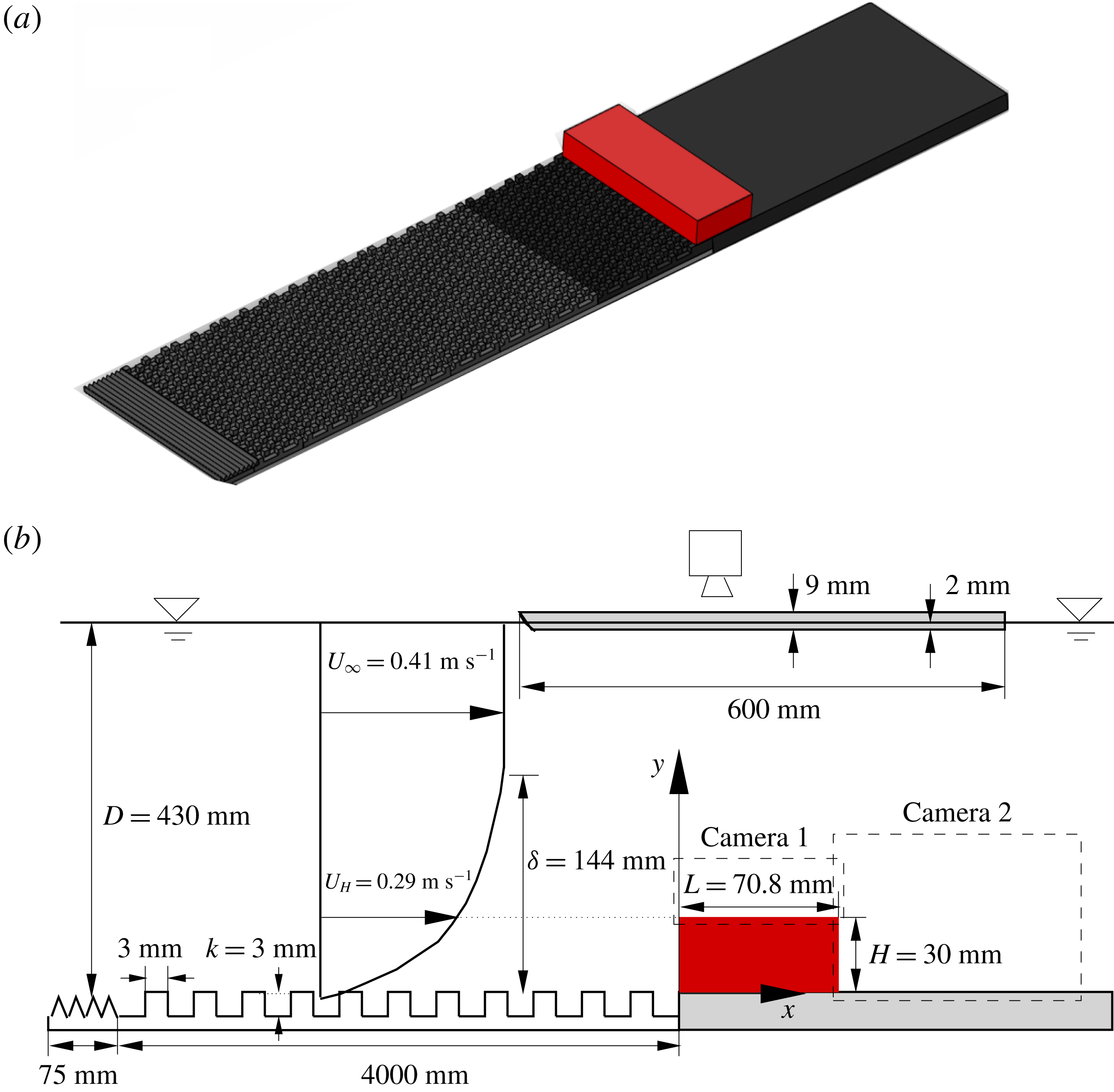
Schematic of experimental set-up and definition of the coordinate system (not to scale): (a) three-dimensional view and (b) side view. The red block is the studied two-dimensional step. The tooth barrier, surface mounted cubes, step and the plate on which the step was mounted all extend the entire spanwise width of the water channel, which is 600 mm. The origin of the
 $z$
coordinate is at the mid-span of the water channel. The marked velocities
 $U_{\infty }$
and
 $U_{H}$
represent the streamwise mean velocities at the free stream and step height, respectively.

Figure 1 illustrates a schematic of the test section as well as the two-dimensional step and coordinate system used in this paper. The instantaneous velocity components along the streamwise (
 $x$
), vertical (
 $y$
) and spanwise (
 $z$
) directions are denoted by
 $u$
,
 $v$
and
 $w$
, respectively. The desired deep upstream TBL was generated using a two-dimensional toothed barrier followed by an array of staggered cubes of height,
 $k=3~\text{mm}$
. The toothed barriers had a height of 15 mm, with triangular cut-outs at the top of pitch 15 mm and depth 12 mm. The cubes were machined from a 6 mm acrylic plate, and had centre-to-centre spacing of 3 mm in both the streamwise and spanwise directions. A three-dimensional representation of the toothed barriers, arrays of cubes and the step used to induce flow separation are shown in figure 1(a). As shown in figure 1(b), the step had a cross-section of
 $30.0~\text{mm}\times 70.8~\text{mm}$
(i.e.
 $L/H=2.36$
), and extended the entire width of the water channel so that its spanwise width (
 $S$
) is 600 mm (i.e.
 $S/H=20.0$
). The step was screwed onto a 6 mm thick acrylic plate with a cross-section of
 $600~\text{mm}\times 600~\text{mm}$
(in the
 $x$
and
 $z$
directions, respectively) that was installed immediately downstream of the cubes. The surface-mounted cubes, the step and acrylic plate on which the latter was screwed were painted with non-reflective black paint to minimize surface glare from laser illumination. All the experiments were performed at a water depth (
 $D$
) of 430 mm and a free-stream velocity (
 $U_{\infty }$
) of
 $0.41~\text{m}~\text{s}^{-1}$
. The room temperature was maintained at
 $20\,^{\circ }\text{C}$
, as such, the kinematic viscosity of the working fluid (
 $\unicode[STIX]{x1D708}$
) was
 $10^{-6}~\text{m}^{2}~\text{s}^{-1}$
. The Reynolds number (
 $Re_{\infty }=U_{\infty }H/\unicode[STIX]{x1D708}$
) and Froude number (
 $U_{\infty }/\sqrt{gD}$
) were 12 300 and 0.20, respectively, where
 $g=9.81~\text{m}~\text{s}^{-2}$
is the acceleration due to gravity. The streamwise mean velocity at the step height is denoted by
 $U_{H}$
. Since the boundary layer thickness is significantly larger than the step height,
 $U_{H}$
is a more appropriate velocity scale than
 $U_{\infty }$
(Castro Reference Castro1979; Lim, Castro & Hoxey Reference Lim, Castro and Hoxey2007), and is used in the subsequent data representation.
2.2 Time-resolved particle image velocimetry (TR-PIV) system
In this research, a planar TR-PIV system was used to measure the velocity field in turbulent flows over the step shown in figure 1. The flow was seeded with 10
 $\unicode[STIX]{x03BC}$
m (
 $d_{p}$
) silver coated hollow glass spheres, which had a specific gravity of 1.4. Following Raffel et al. (Reference Raffel, Willert, Wereley and Kompenhans2007), the slip velocity of particles was estimated from
 $$\begin{eqnarray}U_{s}=\frac{d_{p}^{2}(\unicode[STIX]{x1D70C}_{p}-\unicode[STIX]{x1D70C}_{f})}{18\unicode[STIX]{x1D70C}_{f}\unicode[STIX]{x1D708}}g,\end{eqnarray}$$
where
 $\unicode[STIX]{x1D70C}_{p}$
and
 $\unicode[STIX]{x1D70C}_{f}$
represent the density of the seeding particles and working fluid (water), respectively. The calculated value of
 $U_{s}$
is
 $2.18\times 10^{-5}~\text{m}~\text{s}^{-1}$
, which is orders of magnitude smaller than the smallest velocity scale of the measured fluid motion. Thus, these seeding particles truthfully follow the flow. To quantify the response time of the seeding particles to sudden changes in flow velocity, the relaxation time
 $\unicode[STIX]{x1D70F}_{p}$
was also estimated as
 $$\begin{eqnarray}\unicode[STIX]{x1D70F}_{p}=\frac{d_{p}^{2}(\unicode[STIX]{x1D70C}_{p}-\unicode[STIX]{x1D70C}_{f})}{18\unicode[STIX]{x1D70C}_{f}\unicode[STIX]{x1D708}}.\end{eqnarray}$$
The value of
 $\unicode[STIX]{x1D70F}_{p}$
is
 $2.2\times 10^{-6}$
s. The smallest temporal scale (
 $\unicode[STIX]{x1D70F}_{f}$
) in the studied turbulent flows is estimated to be of the order of
 $\unicode[STIX]{x1D708}/u_{\unicode[STIX]{x1D70F}}^{2}=1.6\times 10^{-3}$
s, where
 $u_{\unicode[STIX]{x1D70F}}$
is the friction velocity, and is approximately
 $0.025~\text{m}~\text{s}^{-1}$
. As such, the Stokes number (
 $S_{k}=\unicode[STIX]{x1D70F}_{p}/\unicode[STIX]{x1D70F}_{f}$
) is about 0.0014, which is within the recommended range of
 $S_{k}\leqslant 0.05$
proposed by Samimy & Lele (Reference Samimy and Lele1991). Therefore, the adopted seeding particles followed the fluid motions very well, and their instantaneous velocities were accurate representation of the instantaneous local fluid velocities.
The flow field was illuminated by a diode pumped dual-cavity dual-head high speed Neodymium-doped yttrium lithium fluoride (Nd:YLF) laser (DM30-527DH, Photonics Industries International, Inc.). Each cavity delivered a maximum pulse energy of
 $30~\text{mJ}~\text{pulse}^{-1}$
at an operation frequency of 1000 Hz (wavelength
 $\unicode[STIX]{x1D706}=527$
nm). This sampling frequency is approximately 1.6 wall units (i.e.
 $f^{+}=f\unicode[STIX]{x1D708}/u_{\unicode[STIX]{x1D70F}}^{2}=1.6$
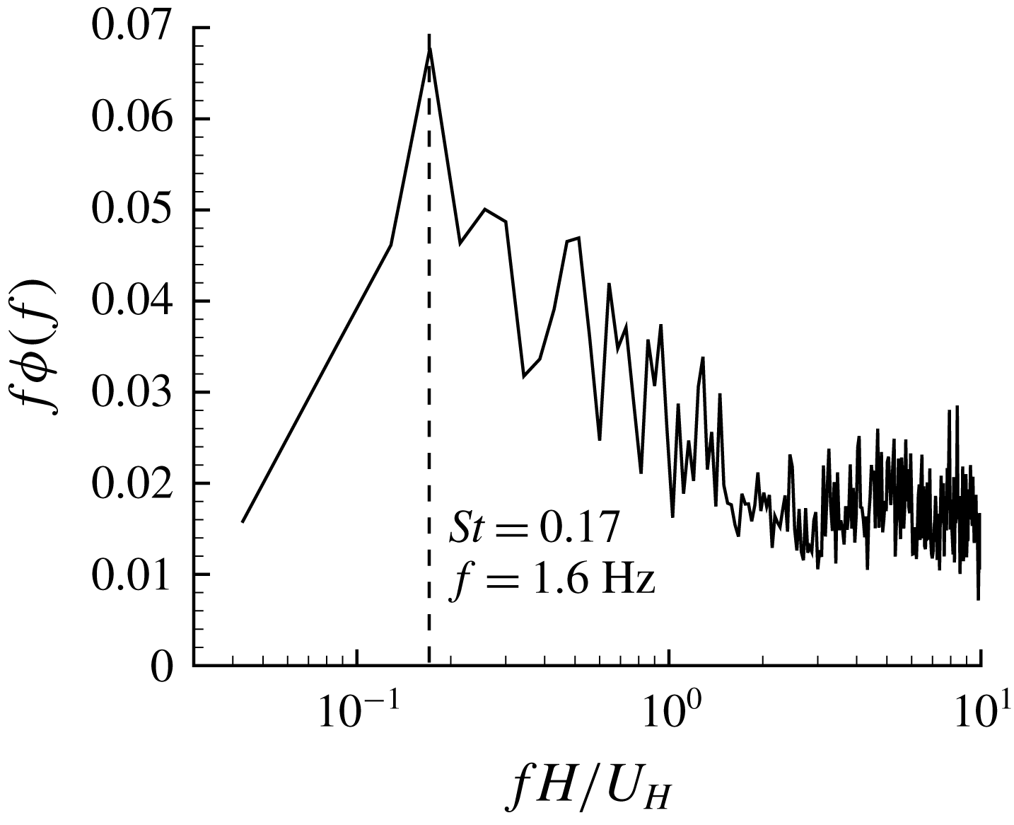
), and is of negligible energy, as will be shown in figure 15. Therefore, the sampling frequency is sufficient to well resolve all temporal scales of importance in this study. A laser sheet of approximately 1 mm thickness was formed by a combination of spherical and cylindrical lenses. The scattered light from the particles was captured by high speed 12-bit complementary metal oxide semiconductor (CMOS) cameras. The cameras were operated at 2560 pixel
 $\times$
1600 pixel (full resolution) and 1920 pixel
 $\times$
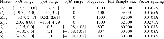
1600 pixel at frame rates of 807 Hz and 1000 Hz, respectively, and were fitted with either a Sigma 105 mm macro lens or a Nikon 60 mm lens, depending on the resolution requirement (see table 1). Both the laser and cameras were installed on a traverse mechanism to facilitate easy and accurate movement to different streamwise locations simultaneously.
The experimental campaign included velocity measurements in the streamwise–vertical (
 $x$
–
 $y$
) plane upstream of the step to quantify the characteristics of the upstream TBL, and subsequently in the
 $x$
–
 $y$
and streamwise–spanwise (
 $x$
–
 $z$
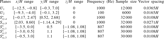
) planes over the step. Details of the measurement planes together with specific information on the field of view (FOV), sampling frequency, sample size, digital resolution and vector spacing are provided in table 1. For the upstream boundary layer measurements, two sets of measurements were conducted at the mid-span of the water channel without installing the step. The first measurement (
 $U_{1}$
in table 1) used a large FOV
 $(352~\text{mm}\times 220~\text{mm})$
to capture the entire thickness of TBL. In this case, the images were acquired at a rate of 1000 Hz and a reduced resolution of 1920 pixel
 $\times$
1600 pixel in a continuous mode. Next, measurements were carried out using a smaller FOV of
 $160~\text{mm}\times 100~\text{mm}$
(
 $U_{2}$
in table 1) at a rate of 100 Hz and a full resolution (2560 pixel
 $\times$
1600 pixel) in a double-frame mode. This is to achieve a better spatial resolution and reliable quantification of second-order moments for the upstream TBL.
List of measurement planes. Measurements in planes
 $U_{1}$
and
 $U_{2}$
were performed without installing the step. Note that measurements in planes
 $S_{xy,a}^{\ast }$
and
 $S_{xy,b}$
were performed simultaneously. To ensure a higher spatial resolution above the step, a Sigma 105 mm macro lens was used in planes with an asterisk superscript (such as
 $S_{xy,a}^{\ast }$
), and a Nikon 60 mm lens was used in other planes.
The
 $x$
–
 $y$
plane measurements over the step were also located at channel mid-span. For these measurements, two cameras, one fitted with Sigma 105 mm macro lens (
 $S_{xy,a}^{\ast }$
in table 1) and the other with Nikon 60 mm lens (
 $S_{xy,b}^{\ast }$
), were used simultaneously to image the flow field at a sampling rate of 1000 Hz and a resolution of 1920 pixel
 $\times$
1600 pixel. The FOV of these cameras overlapped by
 $13.2~\text{mm}$
. To perform measurement in the
 $x$
–
 $z$
planes (
 $S_{xz,j}^{\ast }$
with
 $j=1$
, 2 and 3), the CMOS cameras were placed above the free surface of the water as schematically shown in figure 1(b). Distortion of the captured images from the surface waves was eliminated by placing a 9 mm thick acrylic plate (with a cross-sectional area of
 $600~\text{mm}\times 600~\text{mm}$
in the
 $x$
–
 $z$
plane) beneath the cameras and submerged into the water by approximately 2 mm. The leading edge of the acrylic plate was rounded to further minimize its influence on the flows. The
 $x$
–
 $z$
plane measurements were performed at a vertical distance of 0.5
 $H$
above the top plane of the cubes (
 $S_{xz,1}^{\ast }$
) and at 0.1
 $H$
above the step (
 $S_{xz,2}^{\ast }$
and
 $S_{xz,3}^{\ast }$
). It should be noted that the planes
 $S_{xz,1}^{\ast }$
and
 $S_{xz,2}^{\ast }$
measured the upstream boundary layer at different elevations, whereas
 $S_{xz,3}^{\ast }$
was used to investigate the turbulent separated flows over the step in the streamwise–spanwise plane. For these
 $x$
–
 $z$
plane measurements (
 $S_{xz,j}^{\ast }$
with
 $j=1$
, 2 and 3), the sampling frequency was set to 807 Hz which allowed the full resolution of the cameras (2560 pixel
 $\times$
1600 pixel) to be used.
The data acquisition was controlled by commercial software (DaVis version 8.4) provided by LaVision Inc. In all cases, the particle image diameter was within the range 2–4 pixels, which is the recommended values for minimizing peak locking (DaVis manual by LaVision Inc.). The velocity vectors were calculated using a multi-pass cross-correlation algorithm. Specifically, the interrogation area (IA) was initialized as 128 pixel
 $\times$
128 pixel with 50 % overlap, and finalized as 32 pixel
 $\times$
32 pixel with 75 % overlap.
2.3 Statistical tools
In this paper, the operators
 $\overline{(\cdot )}$
and
 $\langle \cdot \rangle$
denote temporal averaging and conditional averaging, respectively. The mean velocities are also represented using an upper case for convenience, e.g.
 $\overline{u}\equiv U$
. The fluctuating components are denoted by a superscript
 $(\cdot )^{\prime }$
, e.g.
 $u^{\prime }\equiv u-U$
. Other statistical tools used in this paper are summarized in the following subsections for reference.
2.3.1 Correlation
Correlation coefficient is commonly used to quantify spatial/temporal scales (Townsend Reference Townsend1976). It is defined as
 $$\begin{eqnarray}R_{\unicode[STIX]{x1D6F6}\unicode[STIX]{x1D709}}(\boldsymbol{X}_{ref},\unicode[STIX]{x0394}\boldsymbol{X})=\frac{\overline{\unicode[STIX]{x1D6F6}(\boldsymbol{X}_{ref})\unicode[STIX]{x1D709}(\boldsymbol{X}_{ref}+\unicode[STIX]{x0394}\boldsymbol{X})}}{\unicode[STIX]{x1D6F6}_{rms}(\boldsymbol{X}_{ref})\unicode[STIX]{x1D709}_{rms}(\boldsymbol{X}_{ref}+\unicode[STIX]{x0394}\boldsymbol{X})},\end{eqnarray}$$
where
 $\unicode[STIX]{x1D6F6}$
and
 $\unicode[STIX]{x1D709}$
are two general fluctuating components (such as
 $u^{\prime }$
and
 $v^{\prime }$
). In the above equation,
 $\boldsymbol{X}$
and
 $\unicode[STIX]{x0394}\boldsymbol{X}$
denote a general space–time position and a relative displacement, respectively. The subscripts
 $(\cdot )_{ref}$
and
 $(\cdot )_{rms}$
represent the chosen reference point and root-mean-square (r.m.s.), respectively.
2.3.2 Linear stochastic estimation (LSE)
The linear stochastic estimation (LSE) proposed by Adrian & Moin (Reference Adrian and Moin1988) can be used to extract coherent structures associated with a given condition. In the original proposal of LSE by Adrian & Moin (Reference Adrian and Moin1988), an arbitrary number of condition events was employed. However, in the literature, single condition event is the most commonly used approach (e.g. Hambleton, Hutchins & Marusic Reference Hambleton, Hutchins and Marusic2006), and is also employed in this paper. This can be expressed as
 $$\begin{eqnarray}\langle \unicode[STIX]{x1D6F6}(\boldsymbol{x}_{ref}+\unicode[STIX]{x0394}\boldsymbol{x})|E(\boldsymbol{x}_{ref})\rangle =\frac{\overline{E(\boldsymbol{x}_{ref})\unicode[STIX]{x1D6F6}(\boldsymbol{x}_{ref}+\unicode[STIX]{x0394}\boldsymbol{x})}}{E_{rms}^{2}(\boldsymbol{x}_{ref})}E(\boldsymbol{x}_{ref}).\end{eqnarray}$$
The above equation gives an optimal estimation (in terms of the least square error) of a turbulent field solely based on a single-point instantaneous event
 $E(\boldsymbol{x}_{ref})$
.
2.3.3 Proper orthogonal decomposition (POD)
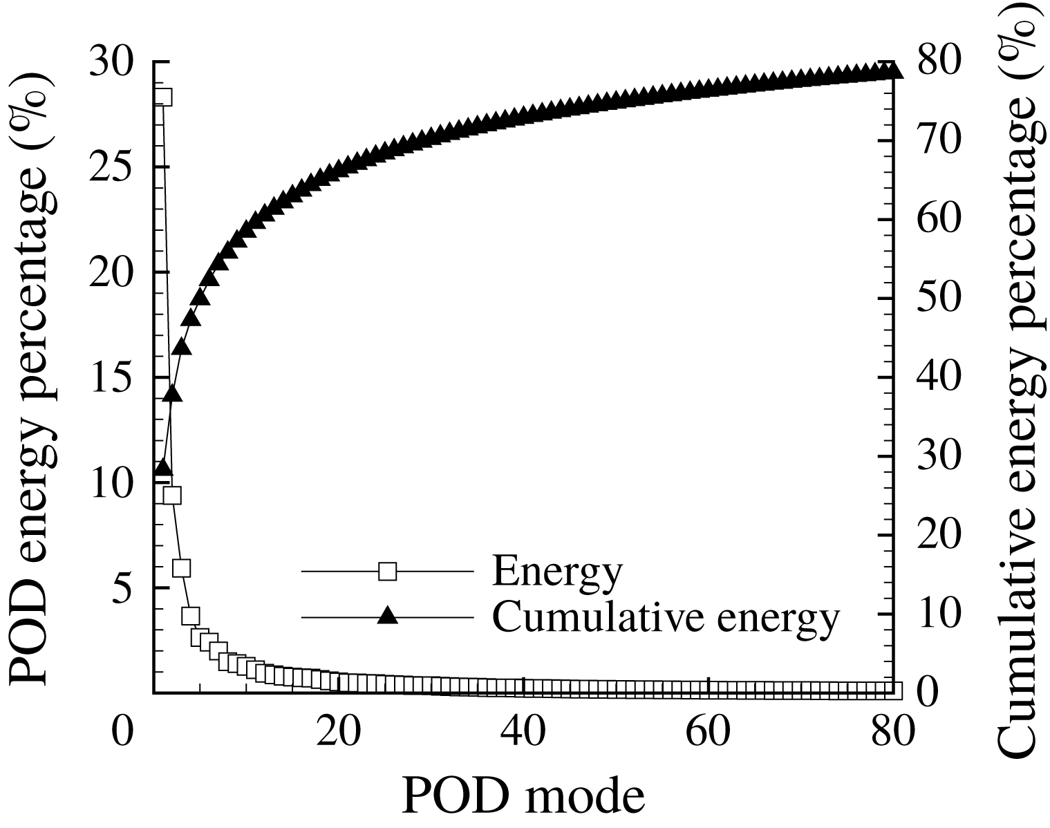
Proper orthogonal decomposition (POD) provides the optimal approximation (in the sense of including the most kinetic energy) for a given number of modes (Berkooz, Holmes & Lumley Reference Berkooz, Holmes and Lumley1993). In POD, the turbulent velocity field is decomposed into different eigenfunctions (or modes) of spatial correlation function (Townsend Reference Townsend1976). In this paper, the fluctuating velocity field is decomposed into different modes as follows:
 $$\begin{eqnarray}\boldsymbol{u}(\boldsymbol{x},t)=\boldsymbol{U}(\boldsymbol{x})+\mathop{\sum }_{j=1}^{M}a^{(j)}(t)\unicode[STIX]{x1D719}^{(j)}(\boldsymbol{x})=\boldsymbol{U}(\boldsymbol{x})+\unicode[STIX]{x1D731}\unicode[STIX]{x1D63C},\end{eqnarray}$$
where
 $\unicode[STIX]{x1D719}^{(j)}$
and
 $a^{(j)}$
represent the
 $j$
th mode (or basis function) and the associated coefficient, respectively, and
 $M$
is the number of modes considered. In the above equation, modes and their coefficients are also expressed using matrix notations as
 $\unicode[STIX]{x1D731}=[\unicode[STIX]{x1D719}^{(1)},\unicode[STIX]{x1D719}^{(2)},\unicode[STIX]{x1D719}^{(3)},\ldots ,\unicode[STIX]{x1D719}^{(M)}]$
and
 $\unicode[STIX]{x1D63C}=[a^{(1)},a^{(2)},a^{(3)},\ldots ,a^{(N)}]^{\text{T}}$
, where
 $N$
is the number of snapshots and the superscript
 $(\cdot )^{\text{T}}$
represents the transpose of a matrix.
Let
 $\unicode[STIX]{x1D733}=[\boldsymbol{u}^{\prime }(t_{1}),\boldsymbol{u}^{\prime }(t_{2}),\boldsymbol{u}^{\prime }(t_{3}),\ldots ,\boldsymbol{u}^{\prime }(t_{N})]$
be an
 $M\times N$
matrix containing all snapshots of fluctuating velocity, and then its singular value decomposition (SVD) is defined as
 $$\begin{eqnarray}\unicode[STIX]{x1D733}=\unicode[STIX]{x1D651}\unicode[STIX]{x1D726}\unicode[STIX]{x1D652}^{\text{T}}.\end{eqnarray}$$
In (2.6),
 $\unicode[STIX]{x1D651}$
is an
 $M\times M$
orthogonal matrix,
 $\unicode[STIX]{x1D652}$
is an
 $N\times N$
orthogonal matrix, and
 $\unicode[STIX]{x1D726}$
is an
 $M\times N$
diagonal matrix. In accordance with (2.5) and (2.6), POD can be simply implemented by letting
 $\unicode[STIX]{x1D731}=\unicode[STIX]{x1D651}$
and
 $\unicode[STIX]{x1D63C}=\unicode[STIX]{x1D726}\unicode[STIX]{x1D652}^{\text{T}}$
. The positively valued diagonal components (denoted as
 $\unicode[STIX]{x1D706}_{j}$
with
 $j=1,2,3,\ldots ,\min (M,N)$
in a descending order) of
 $\unicode[STIX]{x1D726}^{2}$
are eigenvalues of
 $\unicode[STIX]{x1D733}\unicode[STIX]{x1D733}^{\text{T}}$
. As such,
 $\sum _{j=1}^{min(M,N)}\unicode[STIX]{x1D706}_{j}$
is a measure of TKE (for the current planar PIV,
 $M\gg N$
and
 $\sum _{j=1}^{N}\unicode[STIX]{x1D706}_{j}=\int _{{\mathcal{A}}}(\overline{u^{\prime }u^{\prime }}+\overline{v^{\prime }v^{\prime }})\,\text{d}s$
, with
 ${\mathcal{A}}$
representing the area considered in POD). Therefore,
 $\unicode[STIX]{x1D706}_{j}$
represents the contribution of the
 $j$
th POD mode to the integration of TKE in the area (
 ${\mathcal{A}}$
). This implementation of POD is equivalent to that of Meyer, Pedersen & Özcan (Reference Meyer, Pedersen and Özcan2007).
2.3.4 Variable-interval time averaging (VITA)
Blackwelder & Kaplan (Reference Blackwelder and Kaplan1976) proposed a so-called variable-interval time-averaging (VITA) approach to quantify a local (in either space or time) intermittence of turbulent motions. (See Kim (Reference Kim1983) for an application of VITA in space. In this paper, we only adopt VITA in time.) In the VITA approach, a local variance of a general turbulence signal (
 $\unicode[STIX]{x1D6F6}(t)$
) in a variable time interval (
 $T$
) is defined as
 $$\begin{eqnarray}\unicode[STIX]{x1D70E}_{\unicode[STIX]{x1D6F6}}(t,T)=\frac{1}{T}\int _{t-(1/2)T}^{t+(1/2)T}\unicode[STIX]{x1D6F6}^{2}(s)\,\text{d}s-\left(\frac{1}{T}\int _{t-(1/2)T}^{t+(1/2)T}\unicode[STIX]{x1D6F6}(s)\,\text{d}s\right)^{2}.\end{eqnarray}$$
Evidently, for a sufficiently large
 $T$
, the above equation reduces to the calculation of a global variance (
 $\overline{\unicode[STIX]{x1D6F6}\unicode[STIX]{x1D6F6}}$
). Following Bogard & Tiederman (Reference Bogard and Tiederman1986, Reference Bogard and Tiederman1987) and Luchik & Tiederman (Reference Luchik and Tiederman1987), a VITA event (
 $\unicode[STIX]{x1D6F6}(t_{j})$
) is pronounced when
 $\unicode[STIX]{x1D70E}_{\unicode[STIX]{x1D6F6}}(t_{j},~T)>0.4\overline{\unicode[STIX]{x1D6F6}\unicode[STIX]{x1D6F6}}$
and
 $\text{d}\unicode[STIX]{x1D6F6}/\text{d}t|_{t_{j}}>0$
. To further inform the preceding and subsequent turbulent motions of the detected VITA events, an ensemble average of neighbouring
 $t_{j}$
is calculated as follows:
 $$\begin{eqnarray}\langle \unicode[STIX]{x1D6F6}(\unicode[STIX]{x0394}t)\rangle =\frac{1}{G}\mathop{\sum }_{j=1}^{G}\unicode[STIX]{x1D6F6}(t_{j}+\unicode[STIX]{x0394}t),\end{eqnarray}$$
where
 $G$
denotes the number of detected VITA events.
3 Results and discussion
3.1 Upstream boundary layer
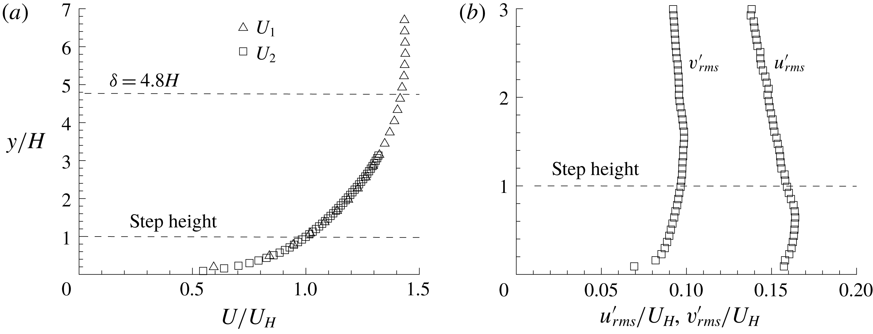
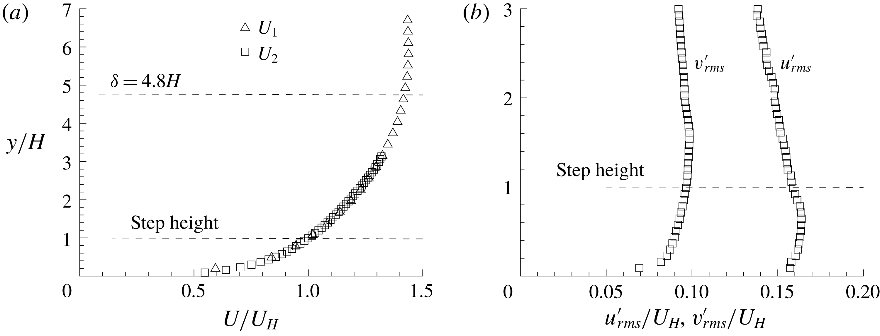
Figure 2 shows the vertical profiles of streamwise mean velocity and r.m.s. of velocity fluctuations for the upstream TBL. The TBL thickness (
 $\unicode[STIX]{x1D6FF}$
) is much larger than the step height (
 $\unicode[STIX]{x1D6FF}=4.8H$
). By fitting
 $U$
profile onto the log law, the friction velocity
 $u_{\unicode[STIX]{x1D70F}}$
is estimated to be
 $0.025~\text{m}~\text{s}^{-1}$
. Therefore,
 $\unicode[STIX]{x1D6FF}^{+}$
(
 $=\unicode[STIX]{x1D6FF}u_{\unicode[STIX]{x1D70F}}/\unicode[STIX]{x1D708}$
) is 3600. Also,
 $H^{+}$
(
 $=Hu_{\unicode[STIX]{x1D70F}}/\unicode[STIX]{x1D708}$
) is 750, and is well into the log-law region, which extends up to
 $y^{+}\approx$
1200.
 $Re_{\unicode[STIX]{x1D703}}$
(
 $=\unicode[STIX]{x1D703}U_{\infty }/\unicode[STIX]{x1D708}$
, where
 $\unicode[STIX]{x1D703}$
denotes the momentum thickness of TBL) is 6900. Due to the deep TBL, the values of
 $u_{rms}^{\prime }$
and
 $v_{rms}^{\prime }$
do not vary significantly (
 $u_{rms}^{\prime }\approx 0.15U_{H}$
and
 $v_{rms}^{\prime }\approx 0.1U_{H}$
) in the region of
 $y/H\in [0,2]$
, where a strong interaction of TBL with the step is expected.
Vertical profiles of (a) streamwise mean velocity and (b) r.m.s. of measured velocity fluctuations. For clarity, every fourth measured point is plotted.
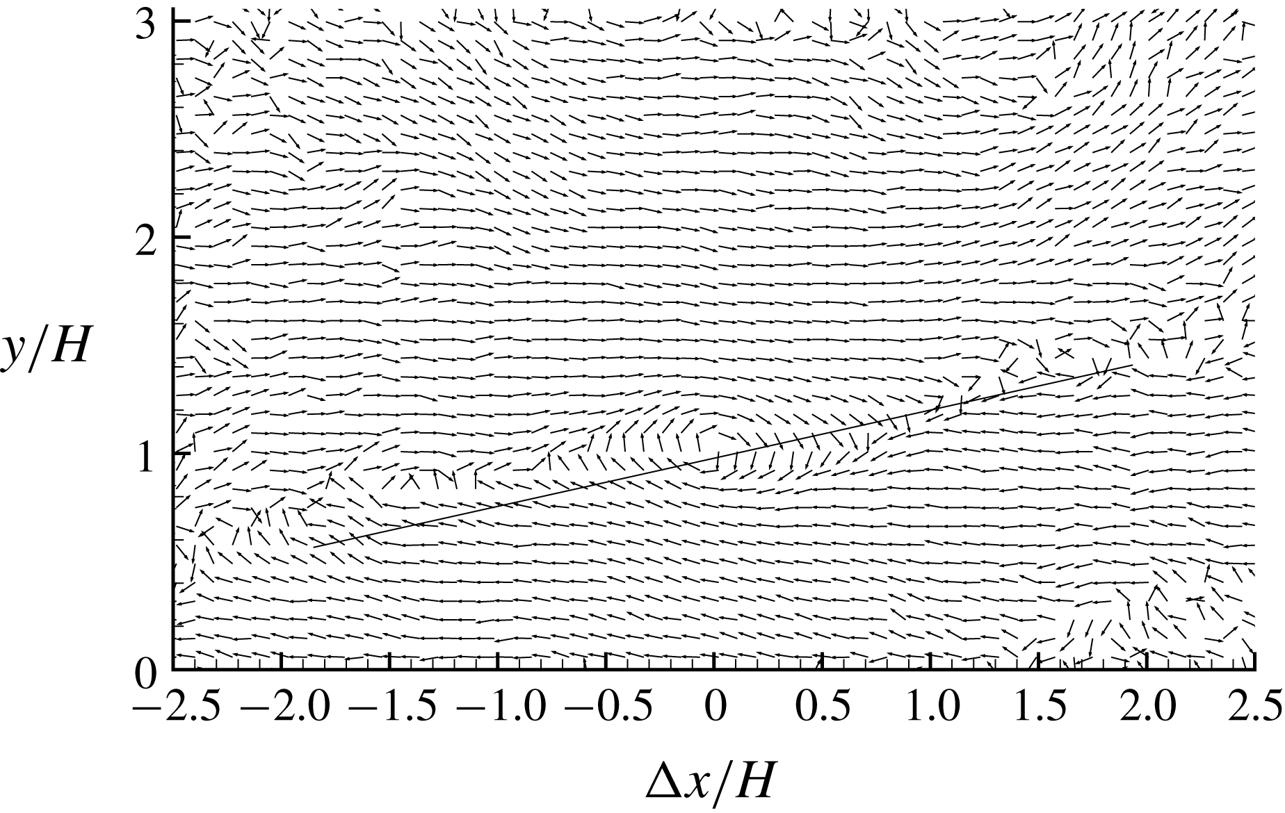
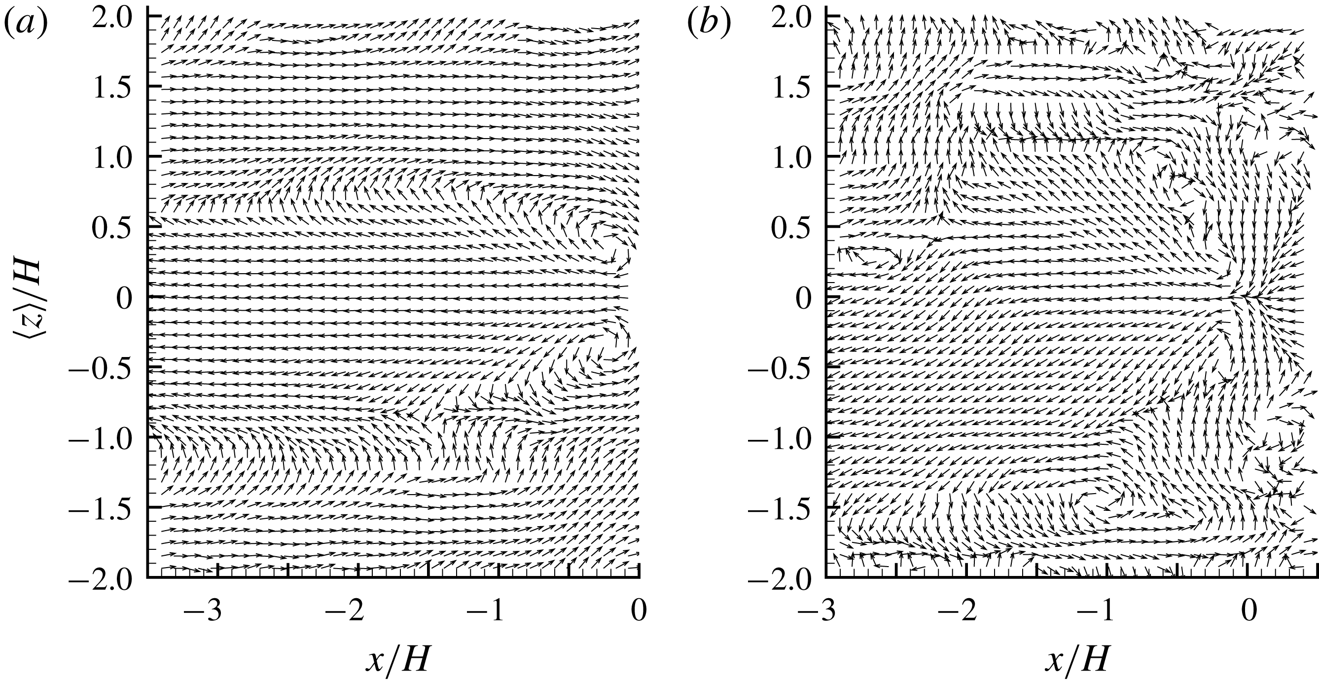
LSE based on the condition of prograde swirling events at step height (
 $y/H=1$
). To facilitate visual inspection, a straight line inclined at
 $13^{\circ }$
is drawn and the vectors are normalized to be of unity length. For clarity, every fourth vector is plotted in both
 $x$
and
 $y$
directions.

Pearson et al. (Reference Pearson, Goulart and Ganapathisubramani2013) observed an enlargement process of reverse flow in front of the step due to the interaction of the step geometry with oncoming low-velocity streaks, which are associated with the ejection event generated beneath the head of a hairpin structure (Zhou et al.
Reference Zhou, Adrian, Balachandar and Kendall1999; Adrian, Meinhart & Tomkins Reference Adrian, Meinhart and Tomkins2000). Inspired by Pearson et al. (Reference Pearson, Goulart and Ganapathisubramani2013), it is worthwhile examining the hairpin structure signature in the upstream flow near the step height because these coherent structures are convected downstream and will eventually interact with the step. Figure 3 shows the LSE of prograde swirling events at the step height for the upstream TBL. Following Christensen & Adrian (Reference Christensen and Adrian2001), a prograde swirling event is defined as
 $\unicode[STIX]{x1D706}_{ci}\unicode[STIX]{x1D714}_{z}/|\unicode[STIX]{x1D714}_{z}|<0$
, where
 $\unicode[STIX]{x1D706}_{ci}$
is the imaginary part of the instantaneous velocity gradient, and
 $\unicode[STIX]{x1D714}_{z}$
represents the instantaneous vorticity in the spanwise (
 $z$
) direction. The pattern of vectors shown in figure 3 is similar to those observed by Christensen & Adrian (Reference Christensen and Adrian2001) and Volina, Schultz & Flack (Reference Volina, Schultz and Flack2009) in TBLs over smooth and rough walls. Specifically, a prograde swirling motion is imposed at the reference point, and multiple smaller swirling motions (more visible if figure 3 is zoomed in without skipping any vectors) occur along a clear inclined edge (as marked by the straight line) extending both upstream and downstream of the reference point. The inclination of the spanwise vortices observed in figure 3 is at
 $13^{\circ }$
, an angle commonly reported in the literature as a signature of hairpin packets (Adrian et al.
Reference Adrian, Meinhart and Tomkins2000; Christensen & Adrian Reference Christensen and Adrian2001; Hambleton et al.
Reference Hambleton, Hutchins and Marusic2006; Volina et al.
Reference Volina, Schultz and Flack2009). It is worth noting here that the marked edge in figure 3 clearly separates areas of positively and negatively valued
 $u^{\prime }$
.
3.2 Turbulence statistics
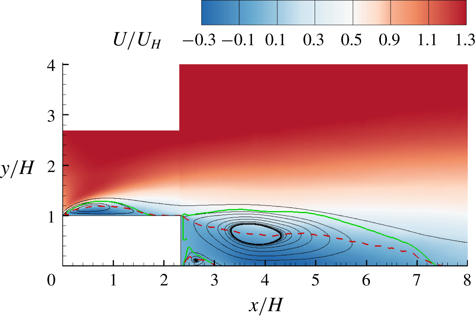
Figure 4 shows the contour of streamwise mean velocity superimposed with mean streamlines. In the figure, three distinct separation bubbles (shown as recirculation regions) can be observed. The small separation bubble in the corner around
 $x/H=2.8$
is not of particular interest. The large separation bubbles over and behind the step, which are the primary focus of this study, are denoted by TSBA and TSBB, respectively, for conciseness in the analysis. The isopleth of
 $50\,\%$
forward-flow fraction
 $\unicode[STIX]{x1D6FE}$
is also plotted, and exhibits a pattern that originates from the leading or trailing edge of the step, passes through the centroid of the separating bubble and terminates on the wall very close to the reattachment points, which is consistent with observations made by Djilali & Gartshore (Reference Djilali and Gartshore1991) and Mohammed-Taifour & Weiss (Reference Mohammed-Taifour and Weiss2016). In figure 4, the isopleth of
 $\unicode[STIX]{x1D6F9}=0$
is also plotted, where
 $\unicode[STIX]{x1D6F9}$
is the integral of streamwise mean velocity in the vertical direction, i.e.
 $\unicode[STIX]{x1D6F9}(x,y)=\int _{wall}^{y}U(x,Y)\,\text{d}Y$
. The isopleth of
 $\unicode[STIX]{x1D6F9}=0$
coincides with the separating streamline (Castro & Haque Reference Castro and Haque1987; Mohammed-Taifour & Weiss Reference Mohammed-Taifour and Weiss2016), which is the mean streamline traced from the leading edge to the reattachment point. Evidently, the isopleths of
 $\unicode[STIX]{x1D6FE}=0.5$
and
 $\unicode[STIX]{x1D6F9}=0$
, respectively, indicate the centre and upper bound of the mean separation bubbles, and therefore are used in subsequent plots as position references whenever applicable.
Contour of streamwise mean velocity (
 $U$
) and mean streamlines. Mean flow reattachment occurs at
 $x/H=1.6$
and 7.4. The superimposed solid and dashed isopleths are
 $\unicode[STIX]{x1D6F9}=0$
and
 $\unicode[STIX]{x1D6FE}=0.5$
, respectively. In this paper, the turbulent separation bubbles over and behind the step are respectively denoted by TSBA and TSBB for conciseness.

TSBA reattaches on the step at
 $x/H=1.6$
. This value is comparable to
 $1.3$
–
 $2.0H$
,
 $1.5$
–
 $2.1H$
,
 $1.82$
–
 $2.04H$
reported by Camussi et al. (Reference Camussi, Felli, Pereira, Aloisio and Di Marco2008), Hattori & Nagano (Reference Hattori and Nagano2010) and Essel & Tachie (Reference Essel and Tachie2017), respectively, for flows over FFS with different turbulent boundary layer thicknesses and Reynolds numbers. In contrast, the reattachment of TSBA is significantly smaller than that (4–5
 $H$
) observed by Bergeles & Athanassiadis (Reference Bergeles and Athanassiadis1983) with an upstream thin boundary layer and low turbulence intensity. The mean reattachment point behind the step is at
 $x/H=7.4$
, i.e.
 $5.1H$
away from the leeward face of the step. The latter distance is comparable to the reattachment length
 $5.05$
–
 $6.54H$
observed by Spazzini et al. (Reference Spazzini, Iuso, Onorato, Zurlo and Di Cicca2001) for a BFS at Reynolds numbers (based on the upstream free-stream velocity and step height) of 3500–16 000.
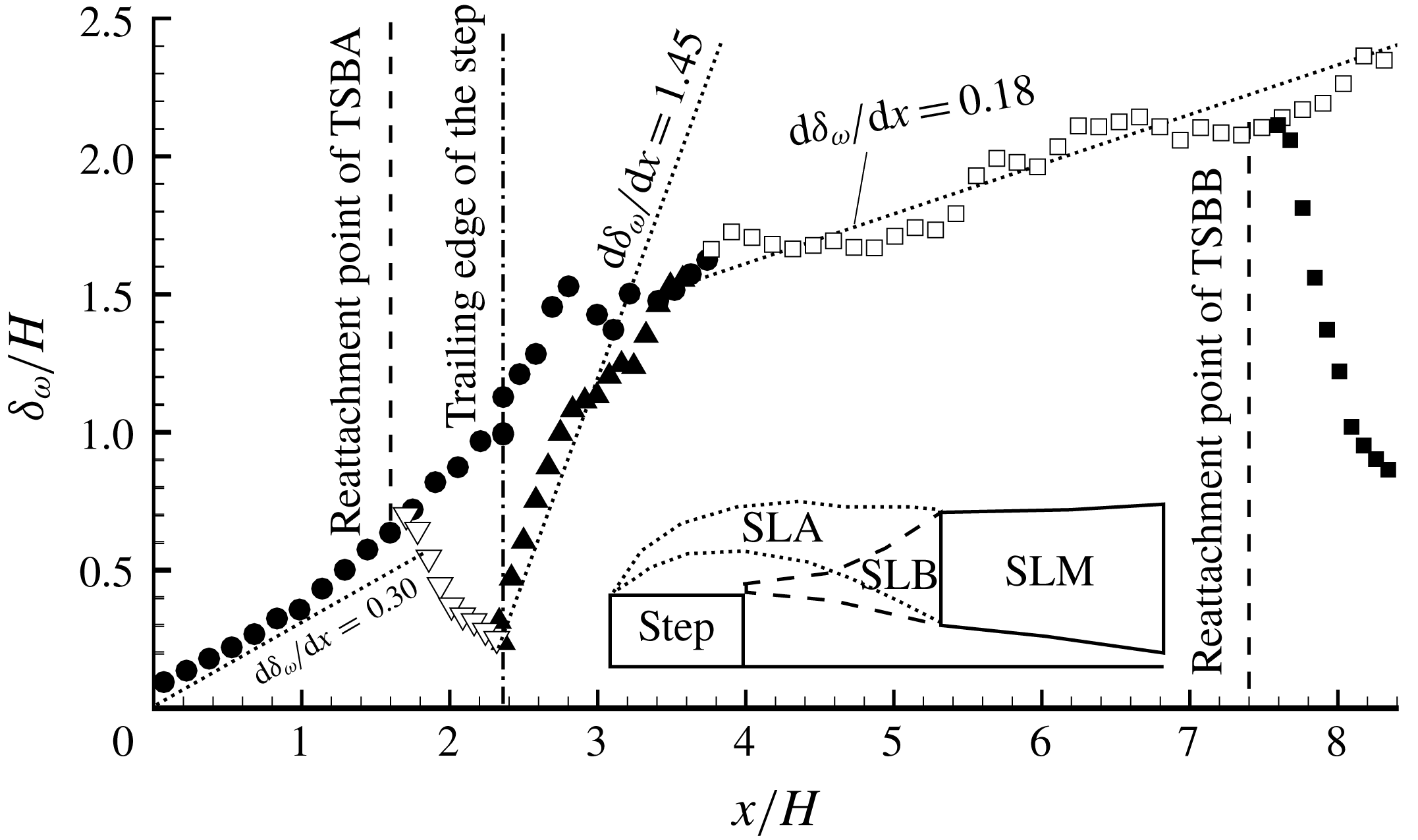
To further analyse the growth of the mean shear layers encompassing TSBA and TSBB, the vorticity thickness, which is defined as
 $\unicode[STIX]{x1D6FF}_{\unicode[STIX]{x1D714}}=(U_{max}-U_{min})/(\unicode[STIX]{x2202}U/\unicode[STIX]{x2202}y)_{max}$
, is employed. Here,
 $U_{max}$
(
 $=U_{\infty }$
) and
 $U_{min}$
denote the maximum (free stream) and minimum streamwise mean velocity, respectively, in the vertical direction. The vorticity thickness was originally proposed by Brown & Roshko (Reference Brown and Roshko1974) for a plane mixing layer, and has since been adopted to quantify the growth of separated shear layers. In fact, many studies have shown that the streamwise development of
 $\unicode[STIX]{x1D6FF}_{\unicode[STIX]{x1D714}}$
along the first half of TSB is very similar to that of a mixing layer. Specifically, it has been observed that
 $\unicode[STIX]{x1D6FF}_{\unicode[STIX]{x1D714}}$
varies linearly with streamwise distance with a slope of
 $\text{d}\unicode[STIX]{x1D6FF}_{\unicode[STIX]{x1D714}}/\text{d}x\in [0.15,0.22]$
for both TSB and mixing layer (Wygnanski & Fiedler Reference Wygnanski and Fiedler1970; Brown & Roshko Reference Brown and Roshko1974; Moss & Baker Reference Moss and Baker1980; Kiya, Sasaki & Arie Reference Kiya, Sasaki and Arie1982; Cherry et al.
Reference Cherry, Hillier and Latour1984; Djilali & Gartshore Reference Djilali and Gartshore1991; Hancock Reference Hancock2000; Lander et al.
Reference Lander, Letchford, Amitay and Kopp2016). In view of the two distinct separation bubbles (TSBA and TSBB) formed due to the intermediate aspect ratio of the step examined herein, there is a need to carefully refine the definition of
 $\unicode[STIX]{x1D6FF}_{\unicode[STIX]{x1D714}}$
to accommodate the possible overlap of shear layers, especially in the region immediately downstream of the trailing edge of the step. We define
 $(\unicode[STIX]{x2202}U/\unicode[STIX]{x2202}y)_{max}$
as local (instead of ‘global’) maximum in the vertical direction, so that multiple peaks of
 $\unicode[STIX]{x2202}U/\unicode[STIX]{x2202}y$
can be captured in accordance with the multiple shear layers.
The topology of the shear layers of the TSBs examined herein is significantly more complex than that over an FFS or downstream of a BFS. In the case of FFS (or BFS),
 $(\unicode[STIX]{x2202}U/\unicode[STIX]{x2202}y)_{max}$
of the shear layer emanating from the leading (or trailing) edge decays in the downstream direction, whereas that of the shear layer initiated by the wall behind the reattachment point increases, and eventually the shear layer away from the wall disappears and a canonical TBL is re-established. Figure 5 shows the streamwise variation of multiple vorticity thicknesses. Evidently, due to the short streamwise extent of the step, a canonical TBL is not established over the step. Immediately downstream of the trailing edge, there exist two shear layers, one emanating from the leading edge (hereafter referred to as SLA) and the other from the trailing edge (hereafter referred to as SLB) (see the inset sketch of figure 5). After
 $x/H\approx 3.5$
, only one peak in
 $\unicode[STIX]{x2202}U/\unicode[STIX]{x2202}y$
is observed, indicating that SLA and SLB merge into a single shear layer, which is denoted by SLM.
Streamwise variation of vorticity thicknesses (
 $\unicode[STIX]{x1D6FF}_{\unicode[STIX]{x1D714}}$
). For clarity, a different number of points are skipped depending on the local cluster of the data points. As shown in the inset sketch (not to scale), the shear layers emanating from the leading and trailing edges of the step (which are, respectively, denoted as SLA and SLB) merge into one shear layer (which is denoted as SLM). Multiple vorticity thicknesses are plotted: solid circles are for SLA; hollow triangles are for wall shear layer developed after reattachment of TSBA; solid triangles are for SLB; hollow squares are for SLM; and solid squares are for wall shear layer developed after reattachment of TSBB.
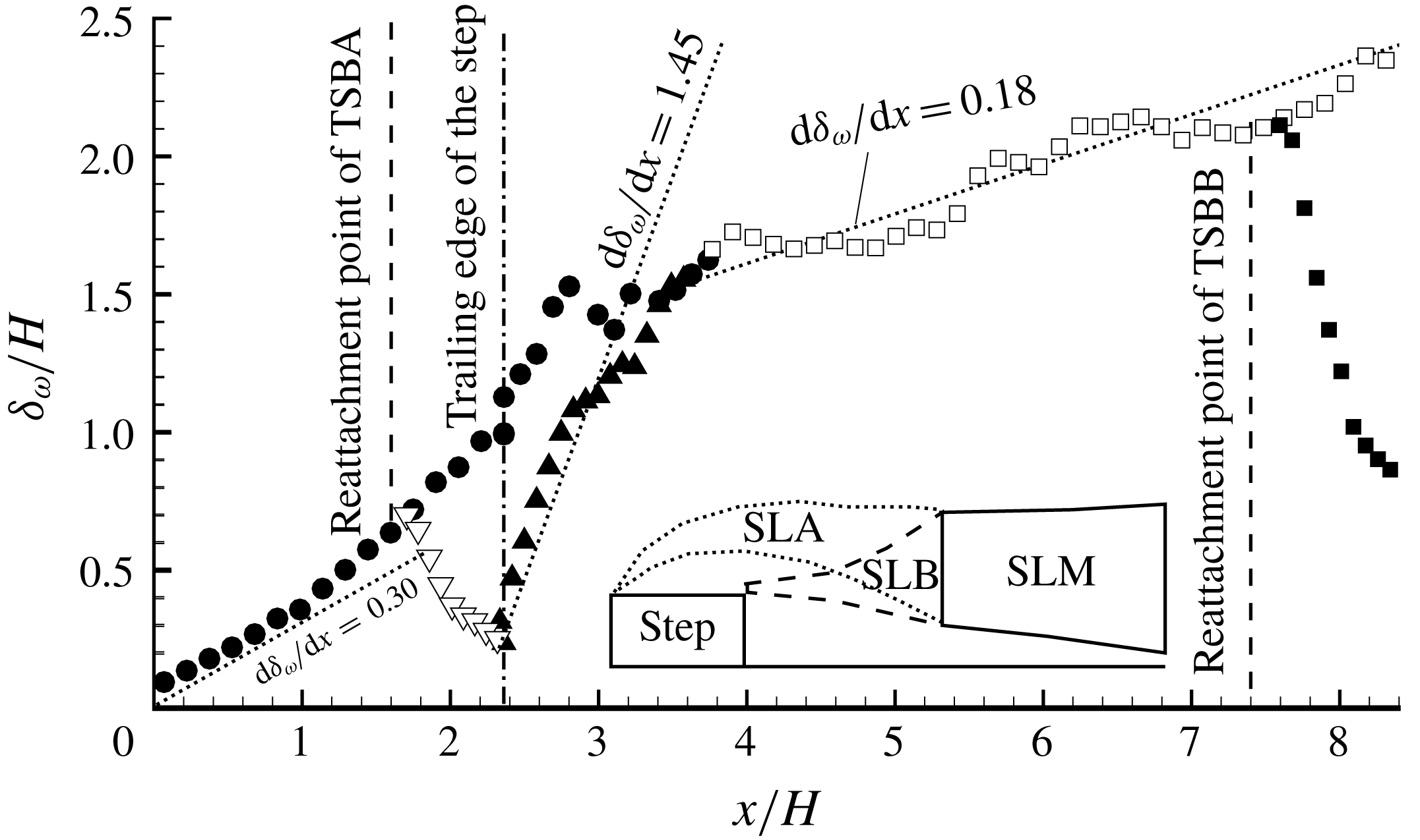
As seen in figure 5, for SLA,
 $\unicode[STIX]{x1D6FF}_{\unicode[STIX]{x1D714}}$
increases linearly with streamwise distance along the front half of the separation bubble (
 $0\leqslant x/H\leqslant 1.0$
) with a slope of
 $\text{d}\unicode[STIX]{x1D6FF}_{\unicode[STIX]{x1D714}}/\text{d}x=0.30$
. This slope is 36–100 % higher than the more commonly reported values of 0.15–0.22 for FFS and BFS, but is in very good agreement with 0.33 observed by Agelinchaab & Tachie (Reference Agelinchaab and Tachie2008) for turbulent flows over a forward–backward-facing step (
 $L/H=6$
) with an upstream deep TBL (
 $\unicode[STIX]{x1D6FF}=9.1H$
) at
 $Re_{\unicode[STIX]{x1D703}}=1800$
. In the region
 $x/H\in [1.0,2.7]$
,
 $\unicode[STIX]{x1D6FF}_{\unicode[STIX]{x1D714}}$
monotonically increases at a faster rate than observed within the first half of the TSBA. This is at variance with the notion that growth rate of
 $\unicode[STIX]{x1D6FF}_{\unicode[STIX]{x1D714}}$
decreases in the rear part of a single separation bubble (Castro & Haque Reference Castro and Haque1987; Djilali & Gartshore Reference Djilali and Gartshore1991; Agelinchaab & Tachie Reference Agelinchaab and Tachie2008). These observations indicate that even though TSBA preserves some of the characteristics of a single separation bubble in the front half, it is noticeably influenced by TSBB in the rear part. It is also apparent from figure 5 that the linear range of
 $\unicode[STIX]{x1D6FF}_{\unicode[STIX]{x1D714}}$
for SLB is very short (approximately
 $x/H\in [2.4,2.8]$
), and its growth rate of 1.45 represents 7-fold to 10-fold typical values (0.15–0.22) reported for an isolated separation bubble behind a BFS. This is a clear manifestation that TSBB is considerably altered by TSBA. It is also interesting to see in figure 5 that the value of
 $\text{d}\unicode[STIX]{x1D6FF}_{\unicode[STIX]{x1D714}}/\text{d}x$
of SLM is approximately 0.18, which is close to that (0.15–0.22) observed in mixing layers (Wygnanski & Fiedler Reference Wygnanski and Fiedler1970; Brown & Roshko Reference Brown and Roshko1974).
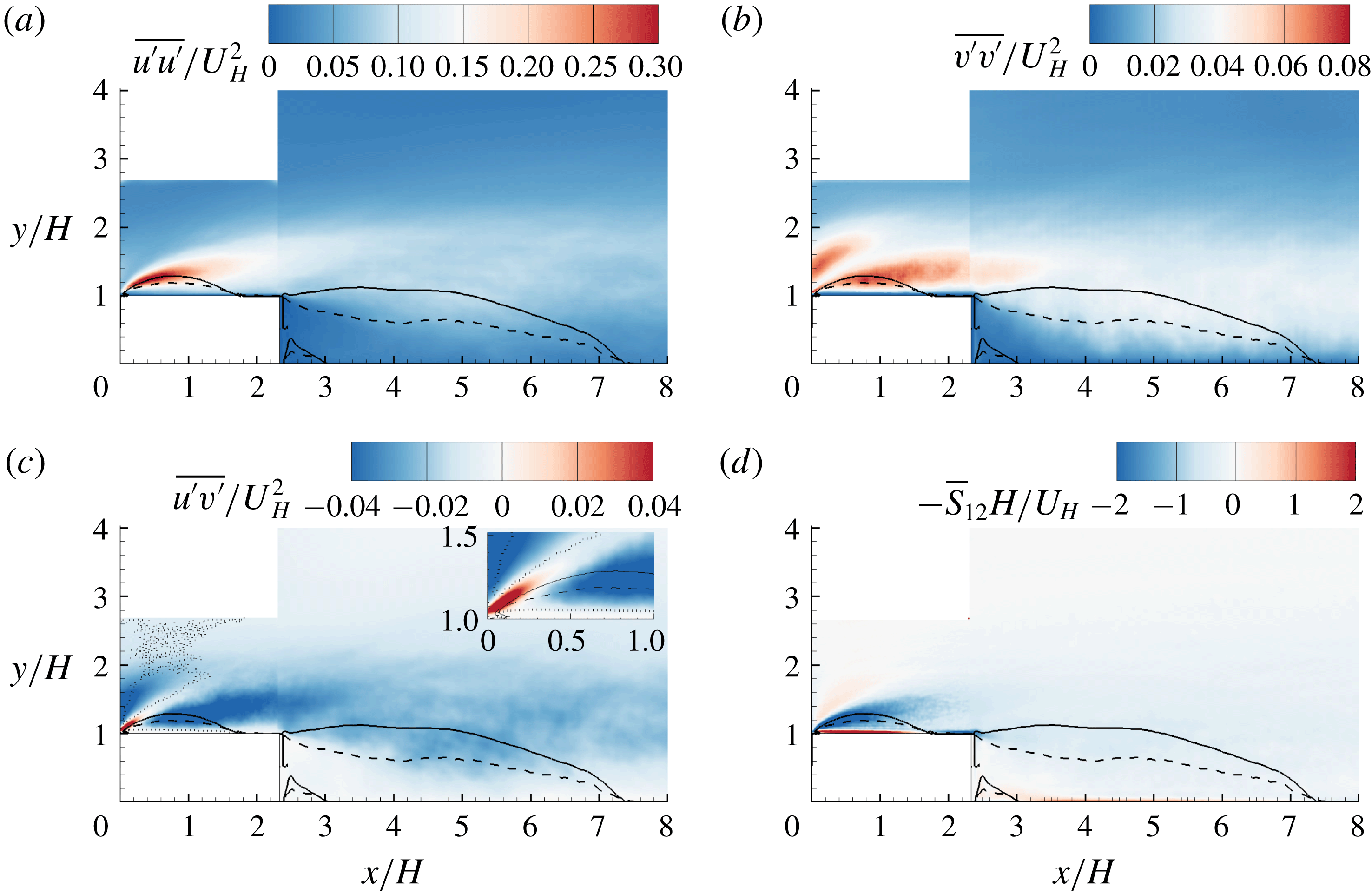
Contours of Reynolds stresses and mean strain rate in the
 $x$
–
 $y$
plane: (a)
 $\overline{u^{\prime }u^{\prime }}$
, (b)
 $\overline{v^{\prime }v^{\prime }}$
, (c)
 $\overline{u^{\prime }v^{\prime }}$
, and (d)
 $-\overline{S}_{12}$
. The superimposed solid and dashed isopleths are
 $\unicode[STIX]{x1D6F9}=0$
and
 $\unicode[STIX]{x1D6FE}=0.5$
, respectively. In (c), the dotted isopleth encompasses the area with negatively valued
 $\overline{S}_{12}$
, and the inset zooms in on the region near the leading edge. Note in (d) that instead of
 $\overline{S}_{12}$
,
 $-\overline{S}_{12}$
is shown to facility visual comparison with
 $\overline{u^{\prime }v^{\prime }}$
.
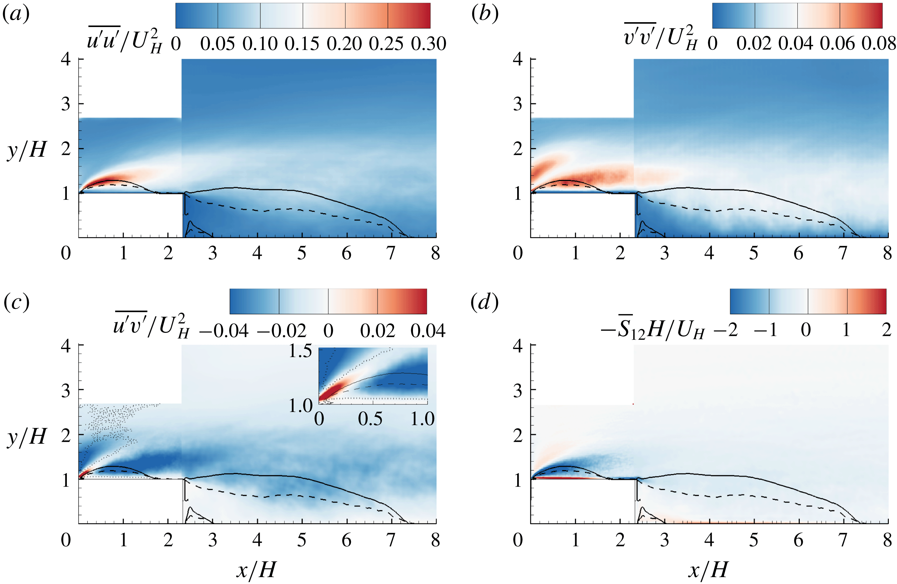
Figure 6(a–c) shows the contours of Reynolds stresses (
 $\overline{u^{\prime }u^{\prime }}$
,
 $\overline{v^{\prime }v^{\prime }}$
and
 $\overline{u^{\prime }v^{\prime }}$
) in the
 $x$
–
 $y$
plane. It is evident from the figures that strong turbulent levels (quantified by all three plotted Reynolds stresses) are apparent near the leading edge of the step (
 $(x/H,y/H)=(0,1)$
, separation point of TSBA), and decrease in the downstream direction. This is remarkably different from turbulent separations with upstream conditions of low turbulence intensity. As an example, for the separation developed over a blunt body with a uniform upstream condition (with characteristic low turbulent intensity), transition to turbulence occurs in the rear part of the separation bubble (Alam & Sandham Reference Alam and Sandham2000; Yang & Voke Reference Yang and Voke2001; Lanzerstorfer & Kuhlmann Reference Lanzerstorfer and Kuhlmann2012). This is also consistent with the experimental observations by Kiya & Sasaki (Reference Kiya and Sasaki1983), Djilali & Gartshore (Reference Djilali and Gartshore1991) and Anand & Sarkar (Reference Anand and Sarkar2017) that
 $u_{rms}^{\prime }$
was trivial near the leading edge and only got amplified in the rear part of separation bubble. Samson & Sarkar (Reference Samson and Sarkar2016) conducted PIV measurements for separation bubbles over a blunt body with different oncoming turbulence intensities. They also observed that a higher approaching turbulence level tends to shift transition to turbulence from the rear part of the separation bubble to the leading edge. The existence of strong turbulence near the leading edge is also reflected by the plotted isopleth of
 $\unicode[STIX]{x1D6FE}$
. It is straightforward that the forward-flow fraction is expected to be either zero or one in a laminar state, which is not observed in any part of separation bubbles shown in figure 6. It follows from the above analysis that the high turbulence intensity from the upstream condition in the present study induces a strong disturbance to TSBA, so that TSBA drifts away from the transition state.
The Reynolds shear stress
 $\overline{u^{\prime }v^{\prime }}$
exhibits some peculiar features that are different to those in a canonical TBL or separation bubble induced by an adverse pressure gradient. With an upstream TBL, Mohammed-Taifour & Weiss (Reference Mohammed-Taifour and Weiss2016) observed that Reynolds shear stress
 $\overline{u^{\prime }v^{\prime }}$
is of a negative sign within the entire separation bubble induced by an adverse pressure gradient, and possesses a peak magnitude above the reattachment point. In contrast, as seen from figure 6(c), strong positively valued
 $\overline{u^{\prime }v^{\prime }}$
appears in an inclined narrow area near the leading edge, where strong positively valued
 $\overline{S}_{12}$
(see figure 6
d) is also observed. This is inconsistent with the Boussinesq eddy-viscosity assumption (BEA), because the BEA predicts that
 $\overline{u^{\prime }v^{\prime }}$
and
 $\overline{S}_{12}$
are of opposite signs, i.e.
 $\overline{u^{\prime }v^{\prime }}=-2\unicode[STIX]{x1D708}_{T}\overline{S}_{12}$
, where
 $\unicode[STIX]{x1D708}_{T}$
is positively valued eddy viscosity. Near the leading edge, a similar contradiction of
 $\overline{u^{\prime }v^{\prime }}$
with the BEA has been observed by Hattori & Nagano (Reference Hattori and Nagano2010) in their DNS study of turbulent flows over an FFS, and also by Essel & Tachie (Reference Essel and Tachie2017) in their experimental study of smooth and rough wall turbulent flows over an FFS.
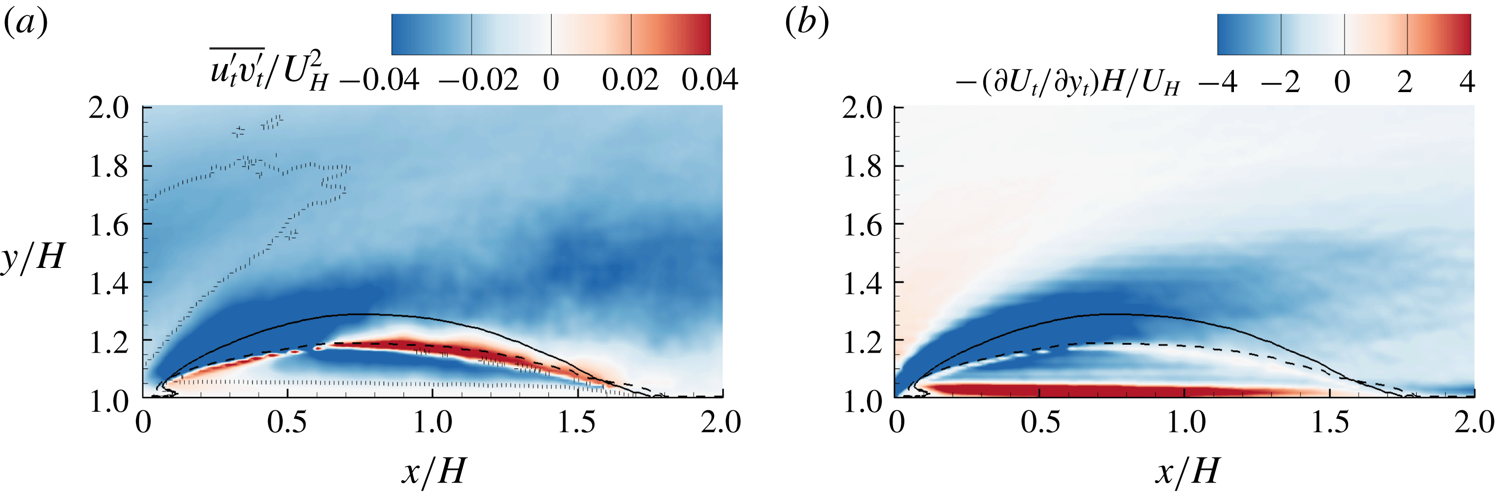
Contours of (a)
 $\overline{u_{t}^{\prime }v_{t}^{\prime }}$
and (b)
 $-\unicode[STIX]{x2202}U_{t}/\unicode[STIX]{x2202}y_{t}$
over the step. The corresponding contours behind the step are not shown to better visualize the dominant variation around the leading edge. The superimposed solid and dashed isopleths are
 $\unicode[STIX]{x1D6F9}=0$
and
 $\unicode[STIX]{x1D6FE}=50\,\%$
, respectively. In (a), the dotted isopleth encompasses the area with negatively valued
 $\unicode[STIX]{x2202}U_{t}/\unicode[STIX]{x2202}y_{t}$
.
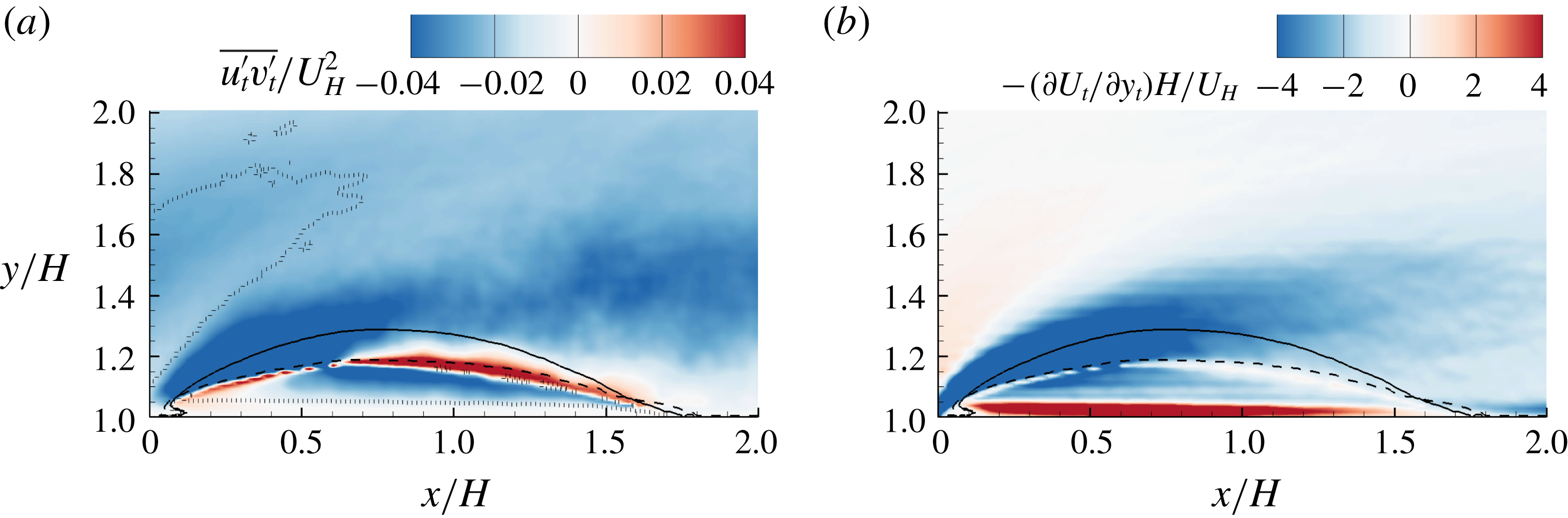
In general, the relationship between Reynolds shear stress and mean strain in turbulent flows with unidirectional mean flow is much easier to predict/model than in separated and reattached turbulent flows with acute streamline curvature. Therefore, we further examine the relationship between Reynolds shear stress and mean strain rate in the curvilinear coordinate system along the mean streamlines. This is to convert the complex separated and reattached mean flow into (at least locally) unidirectional flow in the curvilinear coordinate system. As such, the transformed mean strain reduces to
 $\overline{S}_{12,t}=(\unicode[STIX]{x2202}U_{t}/\unicode[STIX]{x2202}y_{t})/2$
(simply because
 $\unicode[STIX]{x2202}V_{t}/\unicode[STIX]{x2202}x_{t}=0$
based on the definition of streamlines), where subscript
 $(\cdot )_{t}$
denotes the transformed variable,
 $x_{t}$
is along the mean streamline and
 $y_{t}$
axis is
 $90^{\circ }$
with the mean streamline in the anti-clockwise direction. Therefore, along the mean streamlines in the curvilinear coordinate system, the BEA reduces to
 $\overline{u_{t}^{\prime }v_{t}^{\prime }}=-\unicode[STIX]{x1D708}_{T}\unicode[STIX]{x2202}U_{t}/\unicode[STIX]{x2202}y_{t}$
, which is simply Prandtl’s mixing-length hypothesis (PMH) (Prandtl Reference Prandtl1925). Indeed, within the framework of the PMH,
 $\unicode[STIX]{x2202}U_{t}/\unicode[STIX]{x2202}y_{t}$
is a quantification of the effectiveness of momentum transfer (consequently, Reynolds shear stress generation) by a fluid parcel drifting into different streamlines. The transformed Reynolds shear stress
 $\overline{u_{t}^{\prime }v_{t}^{\prime }}=\overline{u^{\prime }v^{\prime }}\cos 2\unicode[STIX]{x1D703}-(\overline{u^{\prime }u^{\prime }}-\overline{v^{\prime }v^{\prime }})/2\sin 2\unicode[STIX]{x1D703}$
(refer to Mohr’s circle for derivation) is calculated with
 $\unicode[STIX]{x1D703}$
being the angle between velocity vector and the
 $x$
direction. To calculate
 $\unicode[STIX]{x2202}U_{t}/\unicode[STIX]{x2202}y_{t}$
, velocities within
 $3\times 3$
neighbour grids are interpolated into the curvilinear coordinate system, and then a finite difference method is used to calculate the derivative. If the PMH is valid even in separated and reattached flows, we should see that
 $\overline{u_{t}^{\prime }v_{t}^{\prime }}$
and
 $\unicode[STIX]{x2202}U_{t}/\unicode[STIX]{x2202}y_{t}$
are of opposite sign everywhere.
Figure 7 shows the contours of
 $\overline{u_{t}^{\prime }v_{t}^{\prime }}$
and
 $-\unicode[STIX]{x2202}U_{t}/\unicode[STIX]{x2202}y_{t}$
over the step. By comparing figure 7(a) against the inset of figure 6(c), it is evident that the area with strong positively valued
 $\overline{u^{\prime }v^{\prime }}$
near the leading edge is now replaced by strong negatively valued
 $\overline{u_{t}^{\prime }v_{t}^{\prime }}$
. Furthermore, the shear layer along the separating streamline (area of strong positively valued
 $\unicode[STIX]{x2202}U_{t}/\unicode[STIX]{x2202}y_{t}$
emanating from the leading edge in figure 7
b) is associated with strong negatively valued
 $\overline{u_{t}^{\prime }v_{t}^{\prime }}$
. This is consistent with the PMH. Therefore, the positively valued
 $\overline{u^{\prime }v^{\prime }}$
and its inconsistency with the BEA observed in figure 6(c) is merely an artefact of misalignment of the local streamlines with the predefined
 $x$
direction. However, the coordinate transformation performed here also leads to areas where the Reynolds shear stresses are inconsistent with the PMH (featuring the same signs of
 $\overline{u_{t}^{\prime }v_{t}^{\prime }}$
and
 $\unicode[STIX]{x2202}U_{t}/\unicode[STIX]{x2202}y_{t}$
), such as the area encompassed by dashed isopleths in figure 7(a) and in the immediate vicinity of isopleth of
 $\unicode[STIX]{x1D6FE}=0.5$
.
3.3 Interaction between different turbulent separation bubbles
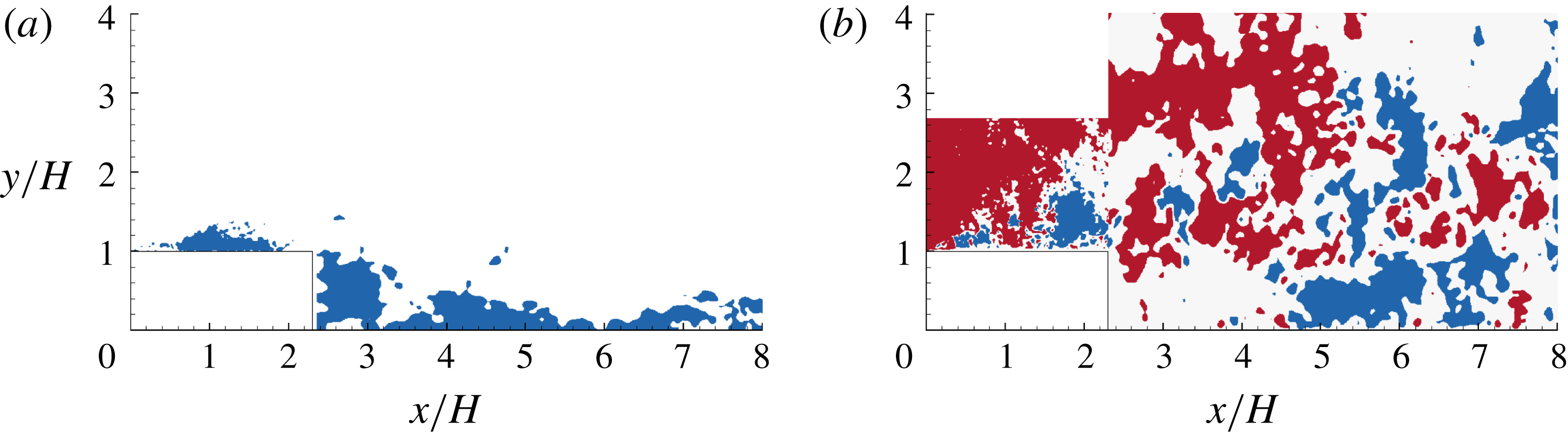
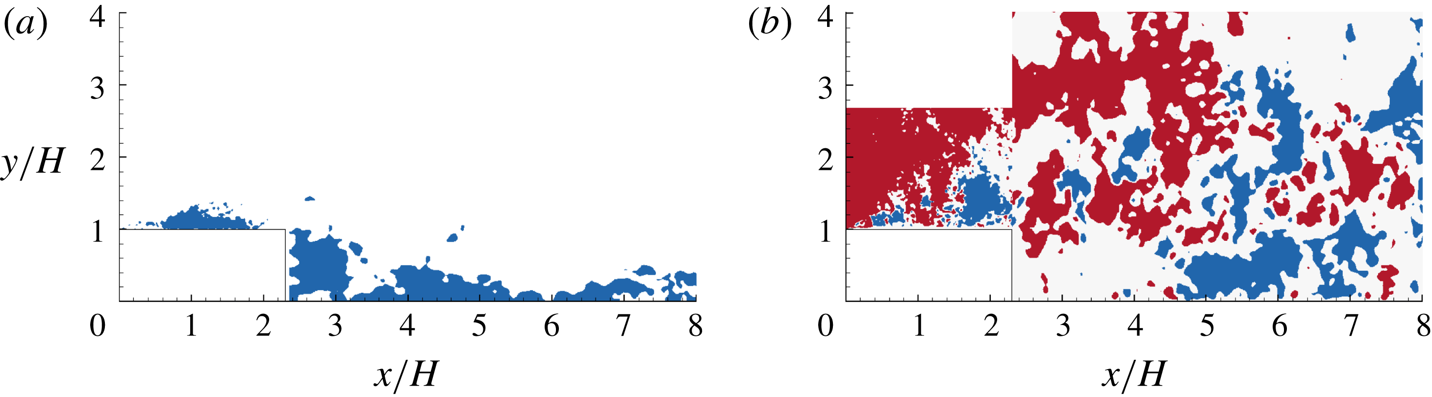
From figure 5, we observed the influence TSBA exerted onto TSBB. In this section, we further investigate the interaction between TSBA and TSBB in more detail. Figure 8 shows an instantaneous velocity field from the simultaneous measurement of TSBA and TSBB (planes
 $S_{xy,a}^{\ast }$
and
 $S_{xy,b}^{\ast }$
in table 1). As seen in figure 8(a), reverse flows commonly appear in irregular shaped areas. The areas of reverse flow are also visible beyond the mean reattachment point. These observations reflect the commonly accepted unsteadiness of reverse flows (Kiya & Sasaki Reference Kiya and Sasaki1983; Cherry et al.
Reference Cherry, Hillier and Latour1984; Le, Moin & Kim Reference Le, Moin and Kim1997; Pearson et al.
Reference Pearson, Goulart and Ganapathisubramani2013). In figure 8(b), areas of alternating positively and negatively valued
 $v$
emanating from the leading edge of the step can be observed, which is reminiscent of spanwise vortex shedding motions. Le et al. (Reference Le, Moin and Kim1997) also observed a similar alternating positively and negatively valued
 $v$
shed from the trailing edge of a BFS. However, the vortices shed from the trailing edge are not visible in figure 8(b), indicating the dominance of vortex shedding from the leading edge. In other words, it is reasonable to expect that TSBB can be directly influenced by the TSBA.
Contours of instantaneous velocity fields. In (a), the blue contour is at
 $u/U_{H}\leqslant 0$
. In (b), the red and blue contours are at
 $v/U_{H}\geqslant 0.1$
and
 $v/U_{H}\leqslant -0.1$
, respectively.
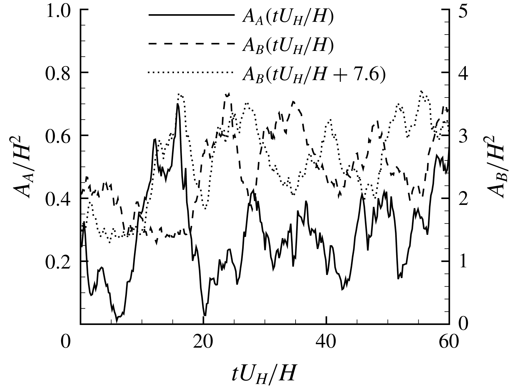
To further investigate the influence of TSBA on TSBB, the areas of reverse flow in TSBA and TSBB (denoted as
 $A_{A}$
and
 $A_{B}$
, respectively) at different times are calculated. It is straightforward to calculate
 $A_{A}(t)$
, i.e. by simply summing up areas of
 $u<0$
above the step. However, some approximation is necessary to find
 $A_{B}(t)$
. The reverse flow induced by the small vortex in the corner behind the step (see figure 4) is not excluded from
 $A_{B}(t)$
, as it is much smaller than TSBB in area. Only the reverse flows in
 $x/H\in [2.3,8.5]$
are accounted for, due to the limitation of our FOV. These approximations are of minor importance in the examination of the interactions of TSBA and TSBB. The reasons are twofold: most reverse flows occur immediately behind the step (see figure 8
a), which is well captured, and the interaction between TSBA and TSBB is expected to be most significant near the trailing edge and decay in the downstream direction.
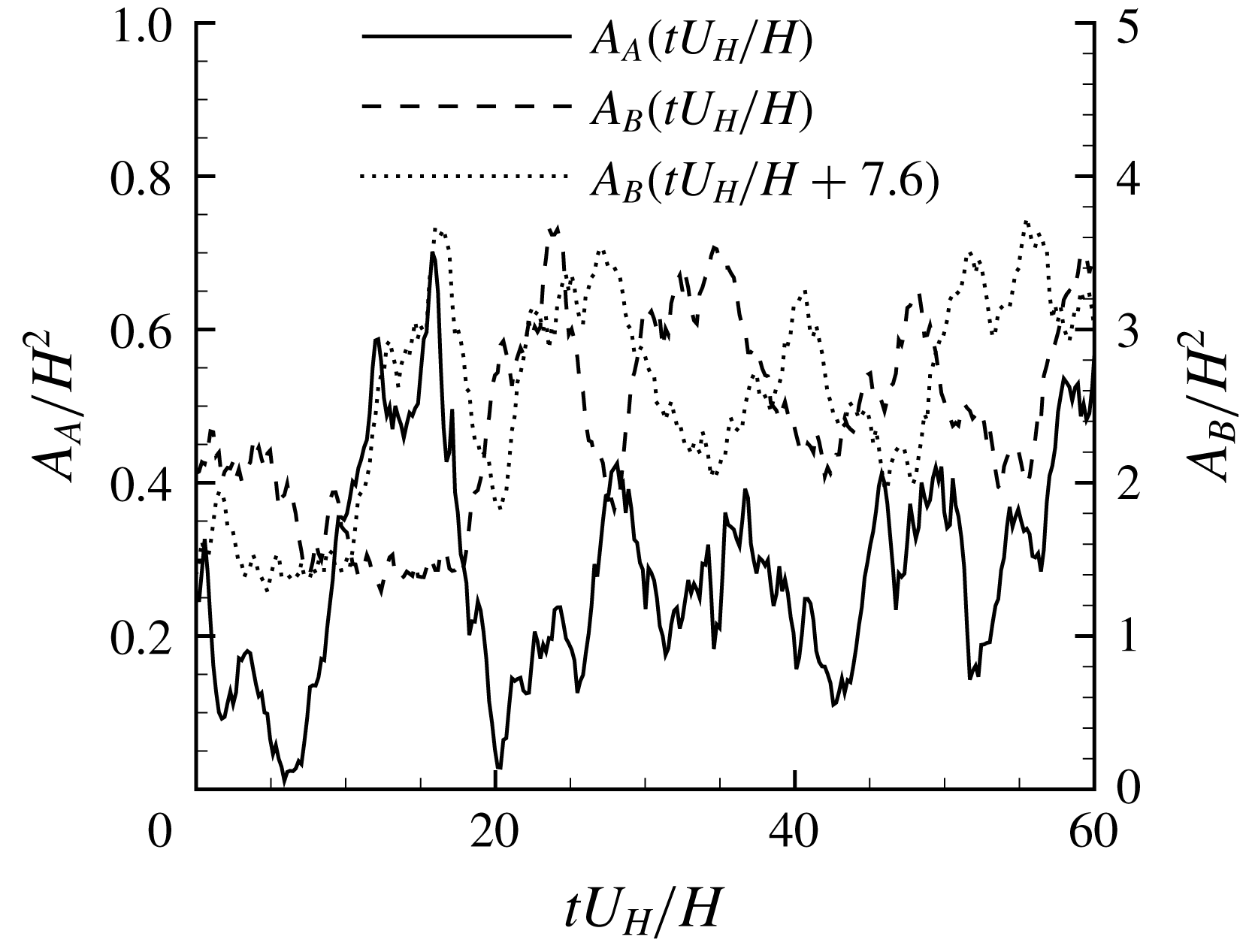
Time sequences of the areas of reverse flow in TSBA and TSBB, denoted as
 $A_{A}$
and
 $A_{B}$
, respectively.
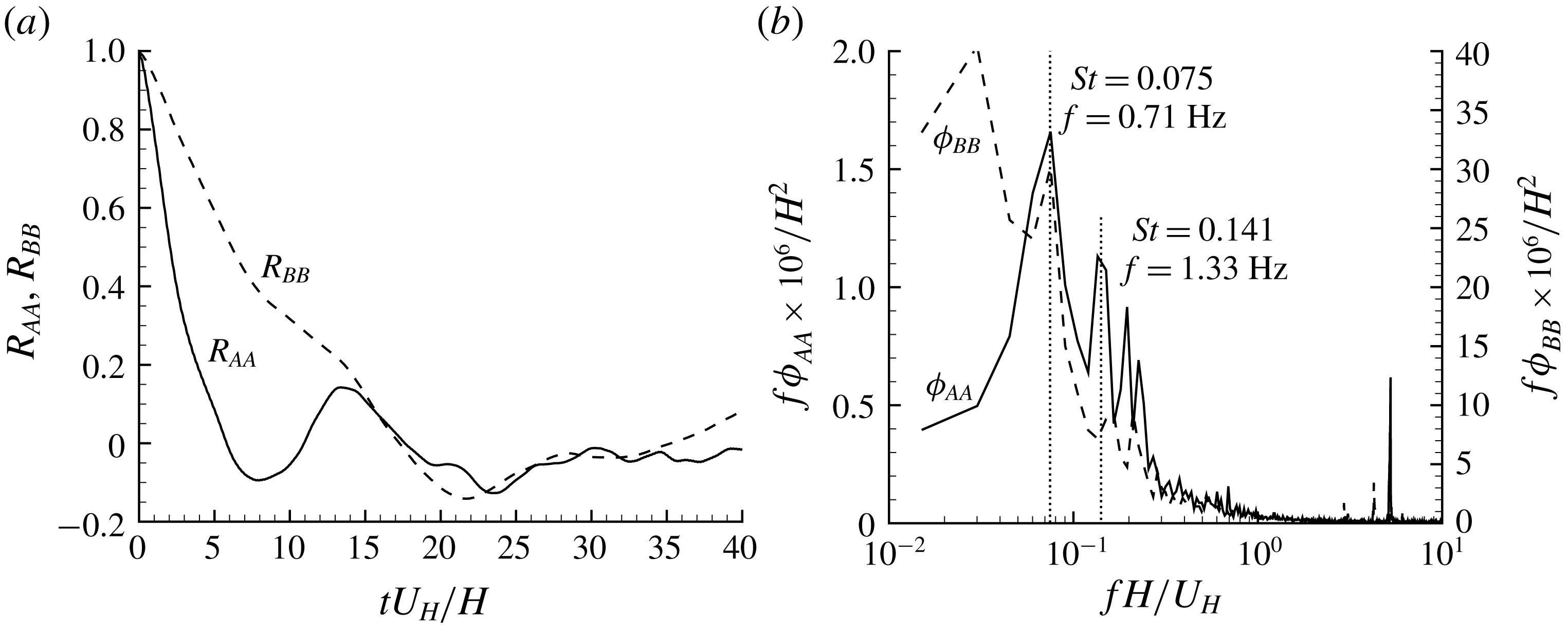
(a) Temporal autocorrelations of
 $A_{A}^{\prime }$
and
 $A_{B}^{\prime }$
(denoted as
 $R_{AA}$
and
 $R_{BB}$
, respectively). (b) Premultiplied frequency spectra of
 $A_{A}$
and
 $A_{B}$
(denoted as
 $\unicode[STIX]{x1D719}_{AA}$
and
 $\unicode[STIX]{x1D719}_{BB}$
, respectively).
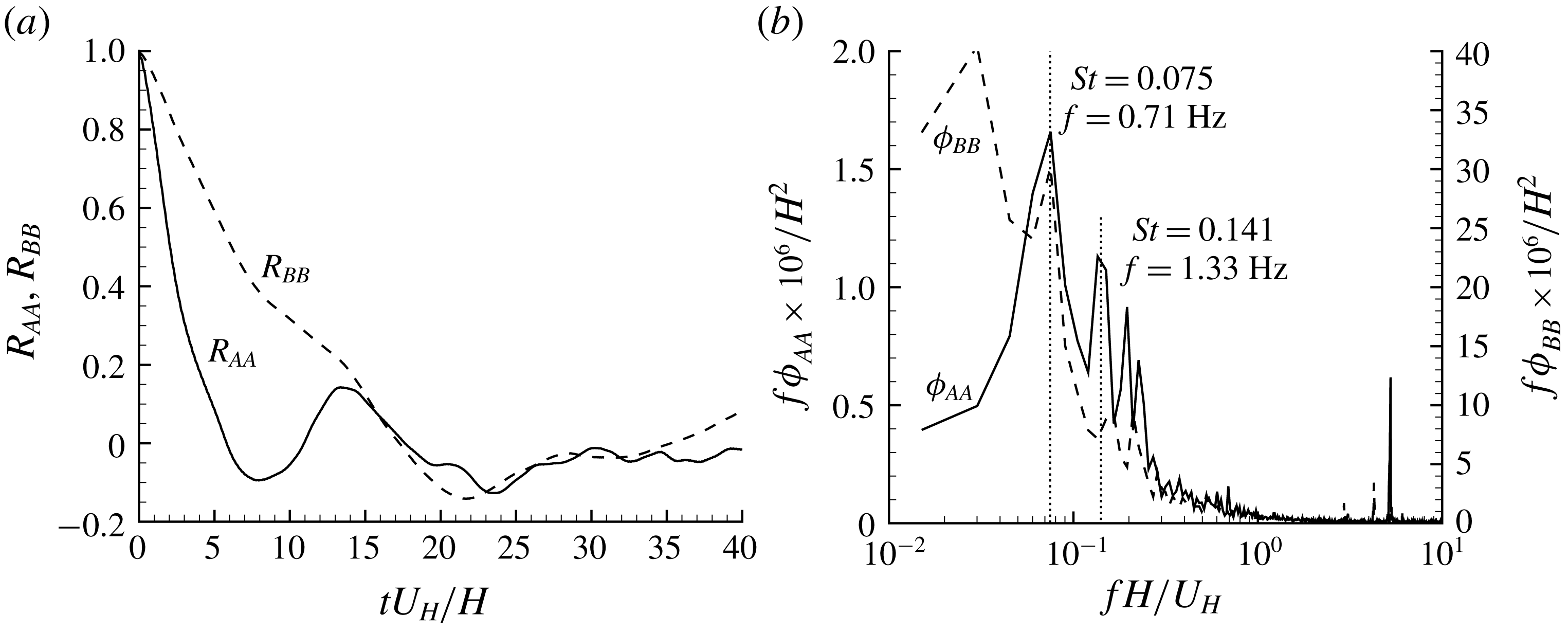
Figure 9 shows sample time variation of the areas of TSBA and TSBB. Evidently, both TSBA and TSBB exhibit strong enlargement/shrinkage fluctuations. To further understand the temporal scales of these two separation bubbles, figure 10 compares the temporal autocorrelations and frequency spectra of
 $A_{A}$
and
 $A_{B}$
. As indicated by the much slower decay rate of
 $R_{BB}$
shown in figure 10(a), the temporal scale of TSBB is much larger than that of TSBA. This is consistent with the observation in figure 10(b). Furthermore, as seen in figure 10(b),
 $f\unicode[STIX]{x1D719}_{AA}$
possesses a sharp peak at
 $St=0.075$
(where the Strouhal number is defined as
 $St=fH/U_{H}$
, following Lim et al. (Reference Lim, Castro and Hoxey2007)), which represents the dominant frequency of the quasi-periodic fluctuation of
 $A_{A}$
, and a subdominant peak at a higher frequency around
 $St=0.141$
. It is interesting to observe that
 $f\unicode[STIX]{x1D719}_{BB}$
also possesses a subdominant peak at
 $St=0.075$
and its global peak is at a much lower frequency (
 $St=0.03$
). It is worth mentioning that
 $St=0.075$
corresponds to
 $f=0.71~\text{Hz}$
in the experiments. With our 32 000 snapshots of images taken at 1000 Hz, approximately 23 periods were captured, which is deemed sufficient to accurately determine the dominance of the corresponding low frequency. However, for the global peak of
 $f\unicode[STIX]{x1D719}_{BB}$
at
 $St=0.03$
, only 9 periods were captured, therefore, its exact value may not be as accurate as the peak frequency of
 $f\unicode[STIX]{x1D719}_{AA}$
.
The dominant frequency of TSBB at
 $St=0.03$
corresponds to
 $fH/U_{\infty }=0.02$
. This value is comparable to
 $fH/U_{\infty }=0.02$
and
 $0.014$
reported by Eaton & Johnston (Reference Eaton, Johnston, Bradbury, Durst, Launder, Schmidt and Whitelaw1982) and Lee & Sung (Reference Lee and Sung2002), respectively, for flows behind a BFS. Considering the significant differences between our flow configuration and those studied by Eaton & Johnston (Reference Eaton, Johnston, Bradbury, Durst, Launder, Schmidt and Whitelaw1982) and Lee & Sung (Reference Lee and Sung2002) (such as Reynolds number and aspect ratio of the step), we conclude that
 $H$
and
 $U_{\infty }$
are, respectively, the appropriate length and velocity scales for TSBB. In other words, TSBB does not scale on
 $U_{H}$
.
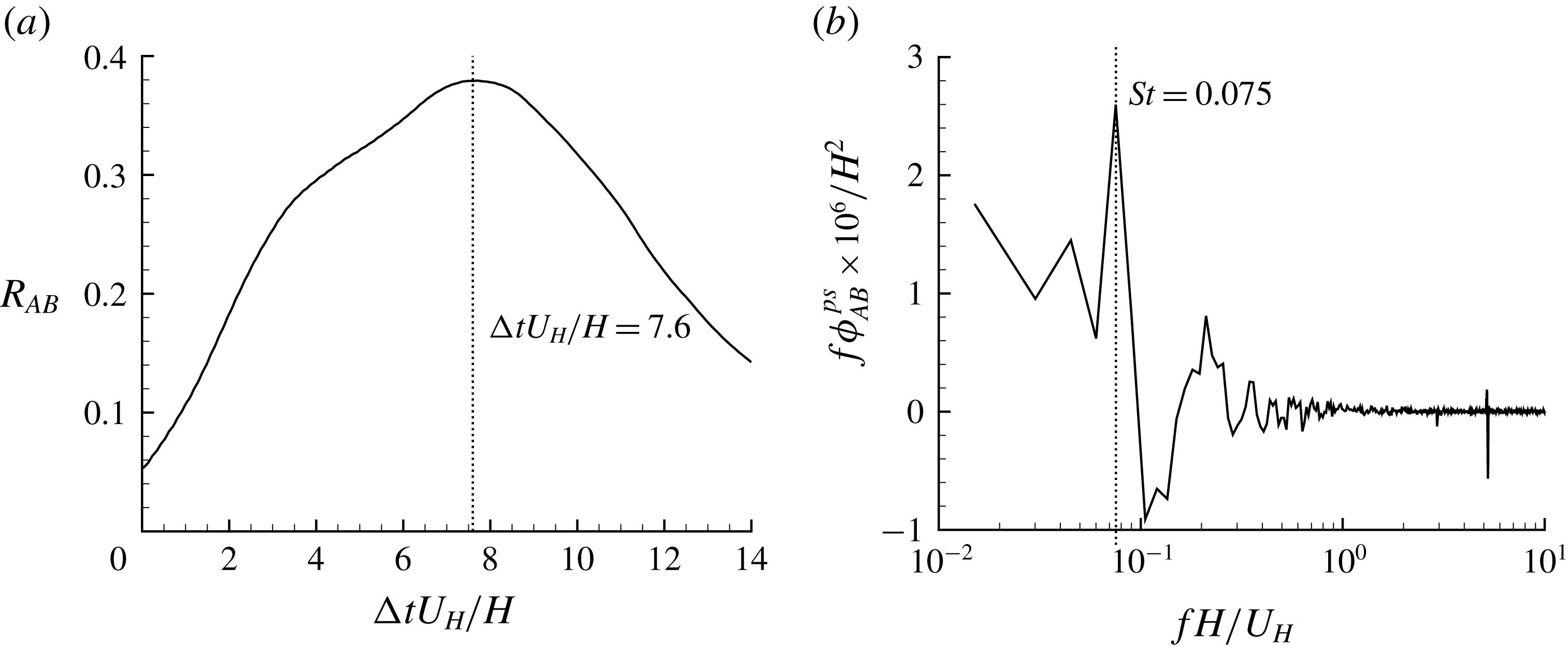
(a) Temporal cross-correlation of
 $A_{A}$
and
 $A_{B}$
(
 $R_{AB}(\unicode[STIX]{x0394}t)$
). (b) Premultiplied phase-shifted co-spectrum
 $\unicode[STIX]{x1D719}_{AB}^{ps}(f,\unicode[STIX]{x0394}t=7.6H/U_{H})$
.

To investigate the modulation of TSBB by TSBA, the temporal cross-correlation of
 $A_{A}$
and
 $A_{B}$
(
 $R_{AB}(\unicode[STIX]{x0394}t)$
) is plotted in figure 11(a). It is interesting to see that the value of
 $R_{AB}(0)$
is as low as 0.05. This is indicative of a poor synchronization of
 $A_{A}$
and
 $A_{B}$
, and is consistent with the observation in figure 9. This may be counter-intuitive because larger
 $A_{A}$
could lead to a stronger momentum deficit over the step, causing a larger TSBB downstream of TSBA. It is interesting to see in figure 11(a) that the value of
 $R_{AB}(\unicode[STIX]{x0394}t)$
increases up to 0.38 as
 $\unicode[STIX]{x0394}tU_{H}/H$
increases to approximately 7.6. This is consistent with the better synchronization between
 $A_{A}(tU_{H}/H)$
with
 $A_{B}(tU_{H}/H+7.6)$
compared to
 $A_{B}(tU_{H}/H)$
as shown in figure 9. This important observation is a clear indication that it takes a considerable time for TSBB to react to the variation of upstream condition induced by TSBA.
In order to further investigate contributions to
 $R_{AB}(\unicode[STIX]{x0394}t)$
from different frequencies, a phase-shifted co-spectrum is defined as follows:
 $$\begin{eqnarray}\unicode[STIX]{x1D719}_{AB}^{ps}(f,\unicode[STIX]{x0394}t)=\overline{\widehat{A_{A}}(f)[\widehat{A_{B}}(f)\exp (2\unicode[STIX]{x03C0}\text{i}f\unicode[STIX]{x0394}t)]^{\ast }}+\overline{\widehat{A_{A}}^{\ast }(f)\widehat{A_{B}}(f)\exp (2\unicode[STIX]{x03C0}\text{i}f\unicode[STIX]{x0394}t)},\end{eqnarray}$$
where
 $\text{i}\equiv \sqrt{-1}$
, and the top-hat
 $\widehat{(\cdot )}$
and superscript
 $(\cdot )^{\ast }$
denote the Fourier transformed coefficient and complex conjugate, respectively. As such,
 $R_{AB}(\unicode[STIX]{x0394}t)=\int \unicode[STIX]{x1D719}_{A}^{ps}(f,\unicode[STIX]{x0394}t)\,\text{d}f$
holds. Apparently, the peak of
 $R_{AB}(\unicode[STIX]{x0394}t)$
is of the most importance. Therefore,
 $\unicode[STIX]{x1D719}_{AB}^{ps}(f,\unicode[STIX]{x0394}t)$
with
 $\unicode[STIX]{x0394}t=7.6H/U_{h}$
is plotted in figure 11(b). It is observed that contents of
 $A_{A}$
and
 $A_{B}$
at high frequencies (say
 $fH/U_{H}>10^{0}$
) are de-correlated (indicated by the trivial magnitudes of
 $f\unicode[STIX]{x1D719}_{AB}^{ps}$
), whereas significant coherency appears at lower frequencies. In particular,
 $f\unicode[STIX]{x1D719}_{AB}^{ps}$
possesses a sharp peak at
 $St=0.075$
. This peak frequency exactly coincides with the peak frequencies observed in figure 10(b). Thus, the peak value of
 $R_{AB}(\unicode[STIX]{x0394}t)$
at
 $\unicode[STIX]{x0394}tU_{H}/H=7.6$
shown in figure 11(a) is primarily induced by the dominant low-frequency oscillation of TSBA. It is also worth mentioning here that the value of
 $\unicode[STIX]{x1D719}_{AB}^{ps}(f=0.075U_{H}/H,\unicode[STIX]{x0394}t=0)$
is trivial (not shown here), reflecting the trivial value of
 $R_{AB}(\unicode[STIX]{x0394}t=0)$
observed in figure 11(a). Based on these observations, it is concluded that TSBA experiences a low-frequency oscillation at a frequency of
 $St=0.075$
, and TSBB mirrors the same oscillation with a time delay of
 $\unicode[STIX]{x0394}tU_{H}/H=7.6$
. In other words, there exists an oscillation between TSBA and TSBB at a frequency of
 $St=0.075$
, and the phase difference between these two separation bubbles is
 $2\unicode[STIX]{x03C0}f\unicode[STIX]{x0394}t\approx 1.1\unicode[STIX]{x03C0}$
.
3.4 Structures in the streamwise–spanwise plane
Pearson et al. (Reference Pearson, Goulart and Ganapathisubramani2013) measured the turbulent separation in front of an FFS. With their measurement data in the
 $x$
–
 $y$
plane, they deduced that the dominant mechanism on the separation is the transverse (spanwise) flow motion along the step, which is affected by the coherent structures in the upstream flow. This deduction is examined with our measurement in the streamwise–spanwise (
 $x$
–
 $z$
) planes at two different elevations (planes
 $S_{xz,j}^{\ast }$
with
 $j=1$
, 2 and 3 in table 1).
Instantaneous velocity fields at
 $y/H$
 $=$
(a) 0.5 and (b) 1.1. The dashed white line indicates the streamwise location of the leading edge of the step. For clarity, every eighth vector is plotted.

Figure 12 shows instantaneous velocity fields at two different
 $x$
–
 $z$
plane measurements. It needs to be pointed out that the streamwise mean velocity (
 $U$
) is always positive at these measurement planes. In other words, the instantaneous reverse flows observed in figure 12 are due to the enlargement of separation bubbles in front of the step. In the vicinity of regions of reverse flow, spanwise flow motions are apparent. Particularly, vertical counter-rotating vortices are observed, and regions of reverse flow are connected with upstream low-velocity regions.
To better reveal the coherent structures associated with the reverse flow, the LSE approach is utilized. The reference point of LSE is chosen at
 $x/H=-0.2$
, a position slightly upstream of the leading edge to capture the spillover of separation. The condition event used in LSE is a local maximum of reverse flow, i.e.
 $u|_{x/H=-0.2}<0$
and
 $u$
at the reference point is smaller than the surrounding eight points. This selected condition event is inspired by Tomkins & Adrian (Reference Tomkins and Adrian2003), who used a local minimum
 $u$
to detect the spanwise centre of low-velocity streaks in a turbulent boundary layer.
LSE velocity fluctuations based on the condition of local maximum reverse flow at
 $x/H=-0.2$
: (a) in the
 $x$
–
 $z$
plane at
 $y/H=0.5$
and (b) in the
 $x$
–
 $z$
plane at
 $y/H=1.1$
. All vectors are normalized to be of unity length. For clarity, every eighth vector is plotted.
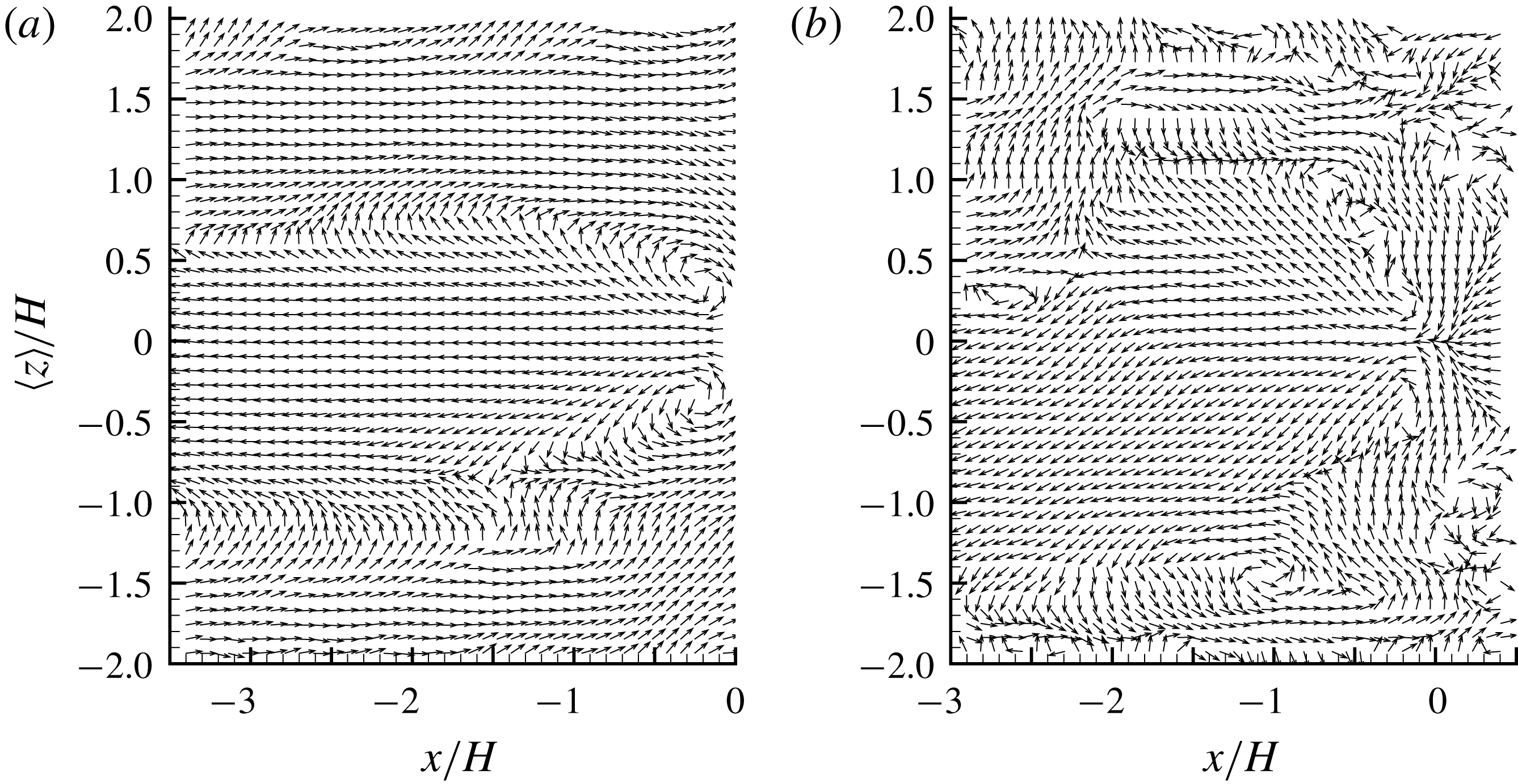
Figure 13 shows the LSE velocity fluctuation fields associated with reverse flows. Evidently, the conditioned reverse flow occurs at the centre of two counter-rotating vortices, and connects with a streamwise-elongated area of negatively valued
 $u^{\prime }$
. This is similar to the structure of near-wall low-velocity streaks in a turbulent boundary layer (Zhou et al.
Reference Zhou, Adrian, Balachandar and Kendall1999; Tomkins & Adrian Reference Tomkins and Adrian2003; Hambleton et al.
Reference Hambleton, Hutchins and Marusic2006). It is also interesting to see in figure 13 that, as the step is approached, the spanwise width of the area of negatively valued
 $u^{\prime }$
becomes narrower. Consequently, the closer counter-rotating vortices also become more efficient in pumping flow in the centre backwards, where reverse flows eventually occur. The above analysis is consistent with the conclusion by Pearson et al. (Reference Pearson, Goulart and Ganapathisubramani2013) that low-velocity streak structure gets stronger as it approaches the step.
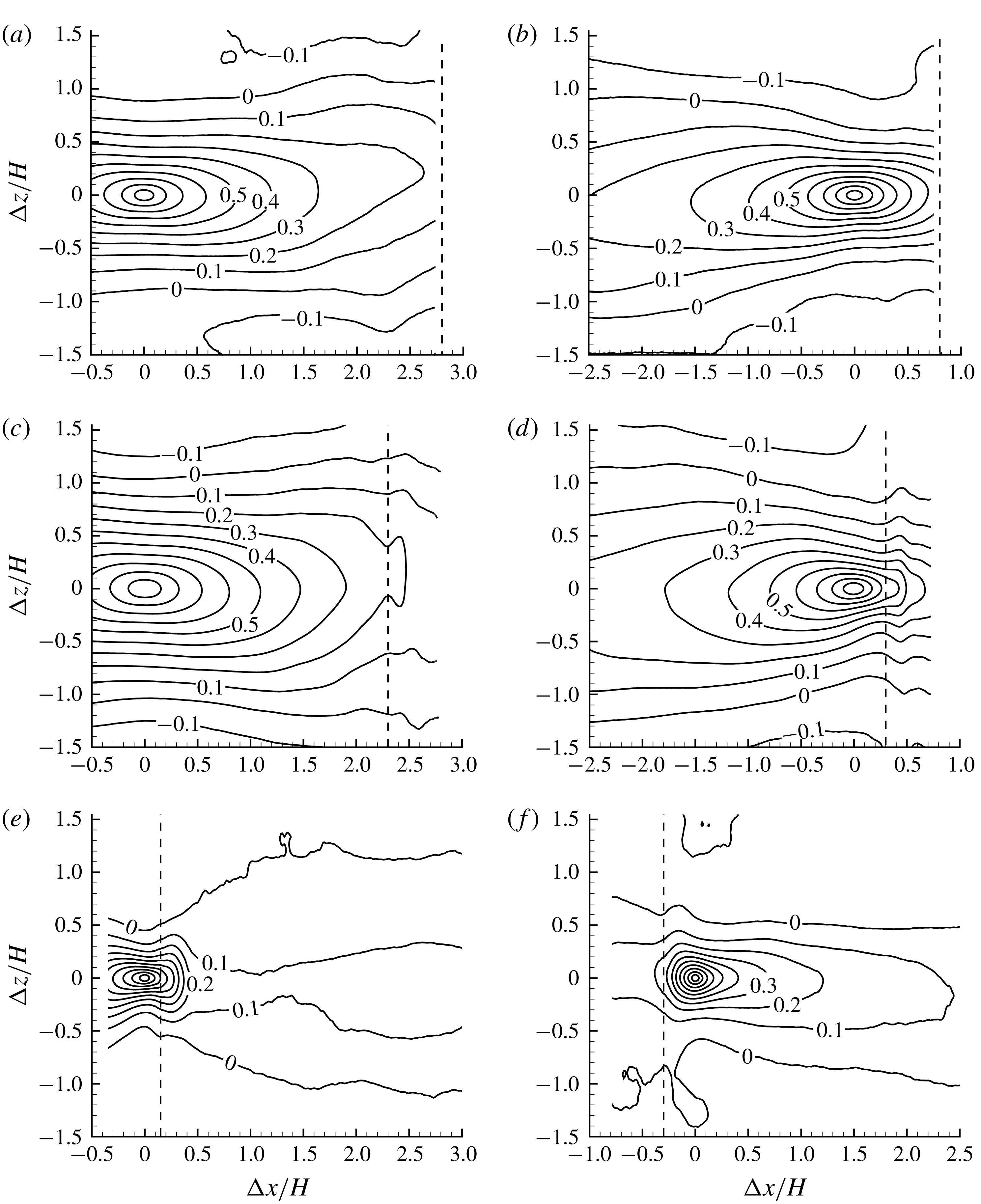
Two-point autocorrelations of streamwise-fluctuating velocities with the reference points chosen at (
 $x/H$
,
 $y/H$
)
 $=$
(a) (
 $-2.8$
, 0.5), (b) (
 $-0.8$
, 0.5), (c) (
 $-2.3$
, 1.1) (d) (
 $-0.3$
, 1.1), (e) (
 $-0.15$
, 1.1) and (f) (0.3, 1.1). The dashed lines mark the position of the leading edge of the step. Isopleths from 0.9 to
 $-0.1$
are plotted, and the interval of adjacent isopleths is 0.1.
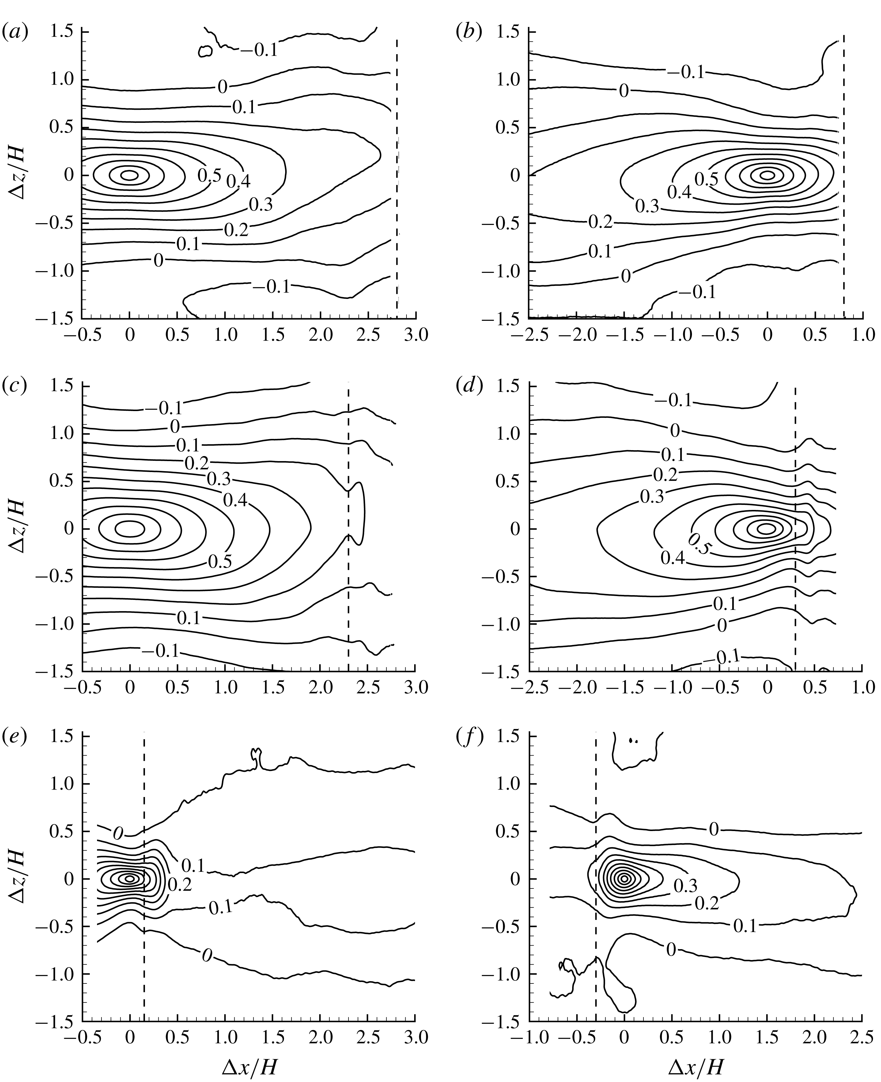
In view of the strong low-velocity structure near the leading edge, it is worthwhile to further investigate the streamwise variation of length scales. To this end, two-point autocorrelations of streamwise-fluctuating velocity (
 $R_{uu}$
) are calculated with different reference points, as shown in figure 14. As seen in figure 14(a,c), the plotted isopleths of
 $R_{uu}$
are well extended in the streamwise direction, and exhibit negative values with sufficient displacement from the reference point in the spanwise direction. This pattern is similar to that in TBL, indicating streamwise-elongated alternating low- and high-velocity streak structures (Volina et al.
Reference Volina, Schultz and Flack2009). By comparing figures 14(b) with 14(a), and 14(d) with 14(c), it appears that, as the step is approached, the isopleths of
 $R_{uu}$
tend to be more clustered together in the spanwise direction. This is consistent with the narrower low-velocity streaks near the leading edge observed in figure 13.
In figure 14(e,f), the reference points are intentionally chosen slightly upstream and downstream of the leading edge, respectively, to show the variation of structures in the vicinity of the leading edge. It is evident that the structures passing the reference point slightly upstream of the leading edge are mostly related to those in the upstream locations. In contrast, the structures slightly behind the leading edge possess a trivial correlation with the upstream locations. It appears that, at the leading edge, there exists a strong destruction mechanism of the upstream coherent structures.
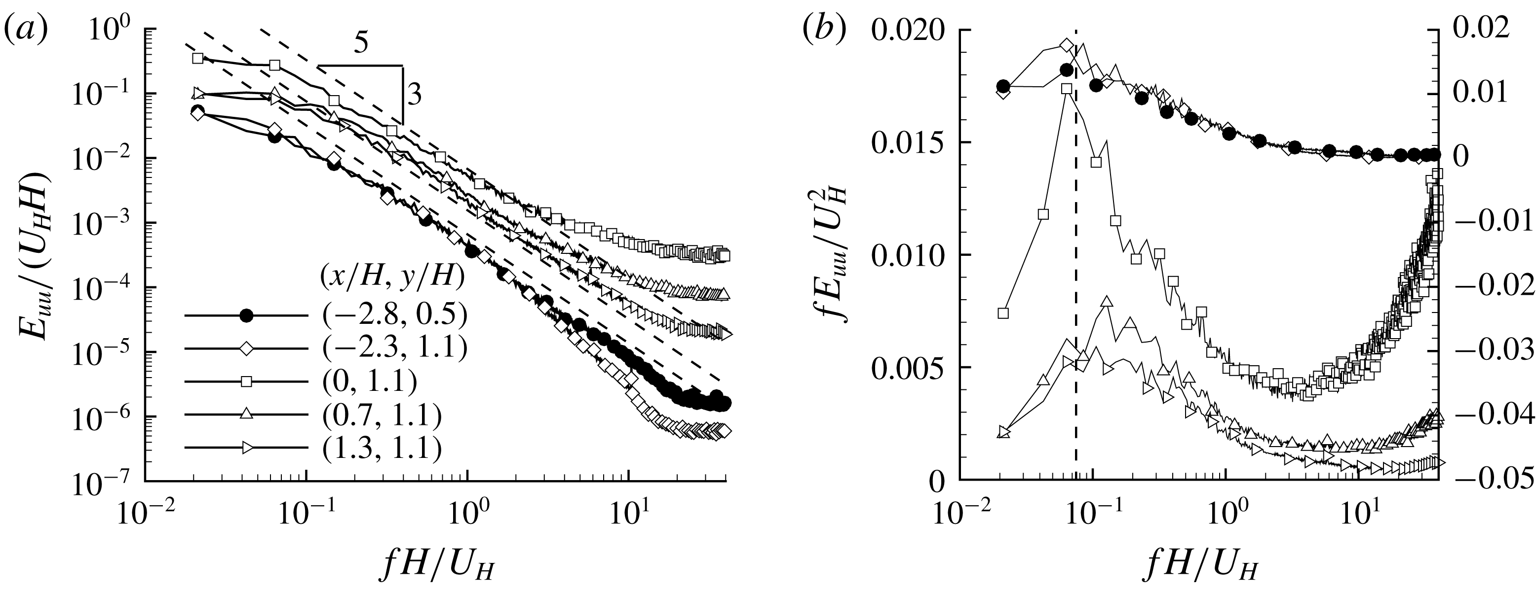
Frequency spectra of streamwise velocity fluctuations at different locations. For clarity, in (b), the premultiplied spectra of points at (
 $x/H$
,
 $y/H$
)
 $=$
(
 $-2.3$
, 1.1) and (
 $-2.8$
, 0.5) use the scale on the right, and the marked dashed line is at
 $St=0.075$
.
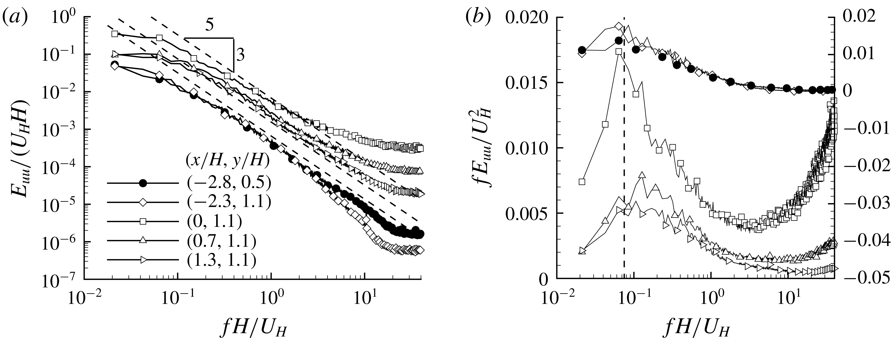
The temporal scales of the velocity fields are further examined in figure 15 using the energy spectrum of streamwise-fluctuating velocity (
 $E_{uu}(f)$
) at different locations. From figure 15(a), the energy held by the highest and lowest frequencies differs by more than three orders of magnitude. This indicates that the current PIV system well captures the entire frequency spectrum, and is indeed time-resolved. The energy spectra in the upstream locations of the step exhibit a wide inertial subrange (featuring the famous
 $-5/3$
slope, see Pope (Reference Pope2000)). This is consistent with the conventional understanding that turbulence tends to be universally isotropic for small scales. As for the energy spectrum directly above the leading edge, the
 $-5/3$
slope is absent and the energy contents at high frequencies are apparently enhanced. This can be attributed to the strong perturbation exerted by the leading edge that breaks the small-scale isotropy. For the position downstream of the leading edge, the
 $-5/3$
slope quickly recovers, a further indication that the leading edge indeed induces small-scale anisotropy.
The dominant frequencies of energy spectra are quantified in figure 15(b) using a premultiplied scale. It is noted that the peak frequencies downstream of the leading edge are higher than those upstream of the step. This is in good agreement with the smaller length scales observed in figure 14 over the step. The peak frequency in the upstream turbulent boundary layer is around
 $St=0.06$
–
 $0.08$
, which is the frequency commonly associated with streamwise-elongated alternating high- and low-velocity streaks. If we assume a convective velocity as
 $0.8U_{\infty }=0.33~\text{m}~\text{s}^{-1}$
,
 $St=0.06$
–
 $0.08$
corresponds to structures with streamwise lengths of
 $430{-}580~\text{mm}\approx 3{-}4\unicode[STIX]{x1D6FF}$
. Monty et al. (Reference Monty, Hutchins, Ng, Marusic and Chong2009) showed that at
 $y/\unicode[STIX]{x1D6FF}>0.265$
(corresponding to
 $y/H=1.27$
in our case) the premultiplied energy spectra of
 $u$
fluctuations in TBL peak around a wavelength of
 $3\unicode[STIX]{x1D6FF}$
. This particular wavelength is also close to the so-called large-scale motion (Adrian et al.
Reference Adrian, Meinhart and Tomkins2000), with a characteristic wavelength of
 $2$
–3
 $\unicode[STIX]{x1D6FF}$
. Overall, the dominant frequency of
 $St=0.06$
–
 $0.08$
, observed in figure 15(b) for the upstream condition, is consistent with that in a canonical TBL.
3.5 Turbulent separation bubble breakup events
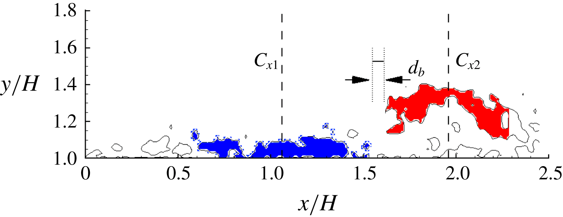
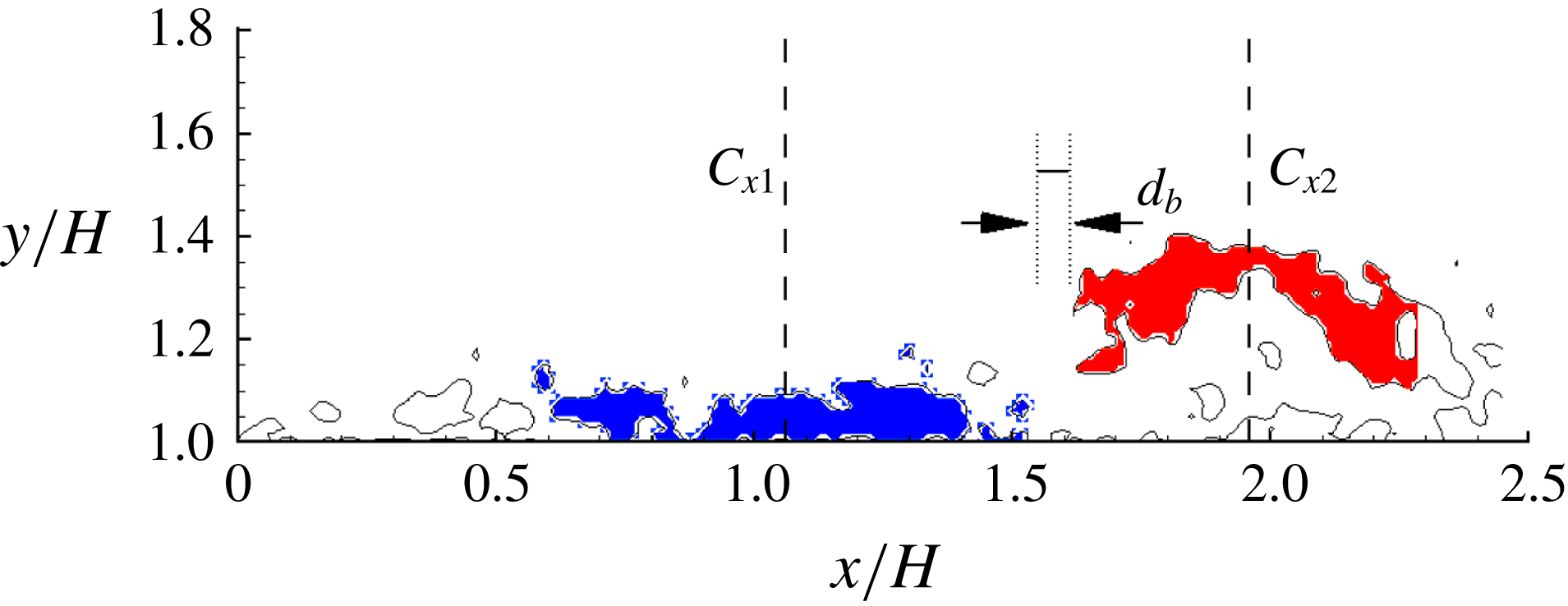
In § 3.3, we analyse the unsteady characteristics of reverse flows without consideration of their discontinuity in space. In this section, we further investigate TSBA from the perspective of separation bubble breakup (SBBU) events. Figure 16 shows a cluster of reverse flows at a different time from figure 8. Figure 16 reveals a flow pattern that is in sharp contrast to figure 8(a). Specifically, in figure 8(a), most of the reverse flow above the step is clearly clustered in a continuous region, whereas figure 16 exhibits a noticeable gap around
 $x/H=1.6$
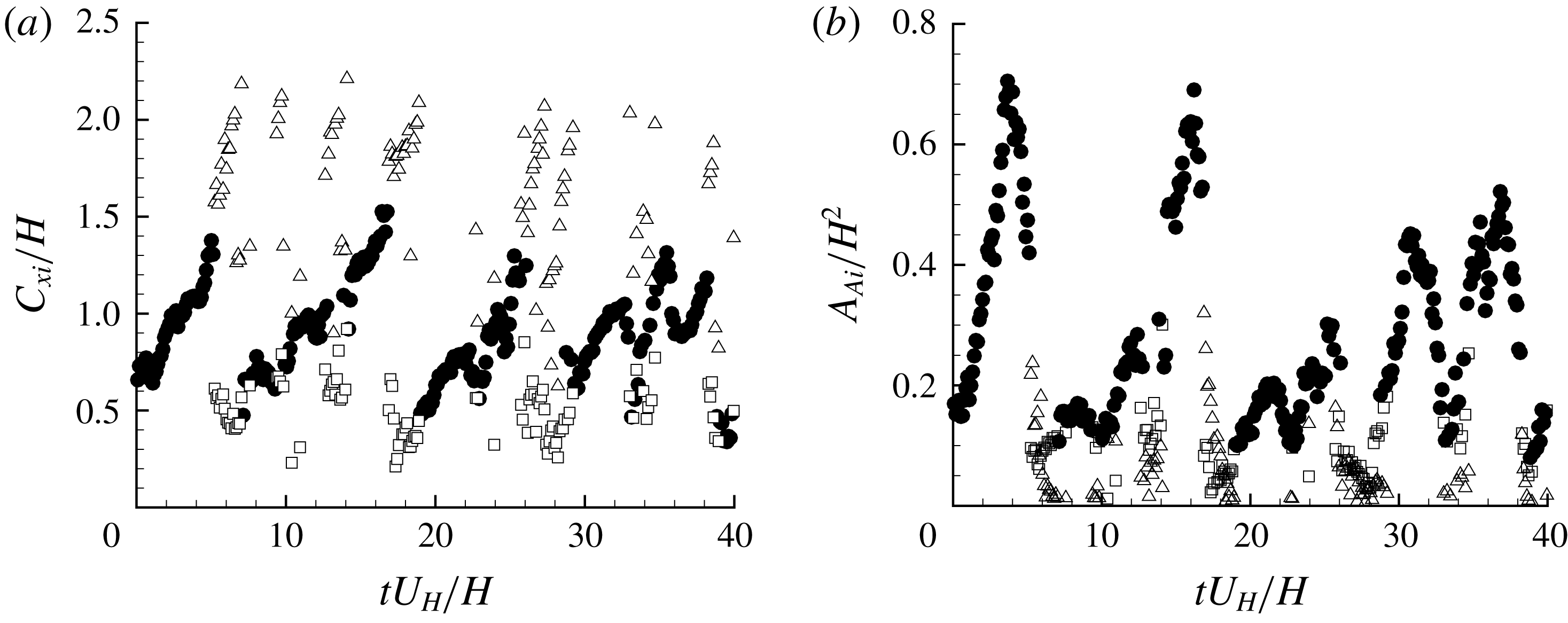
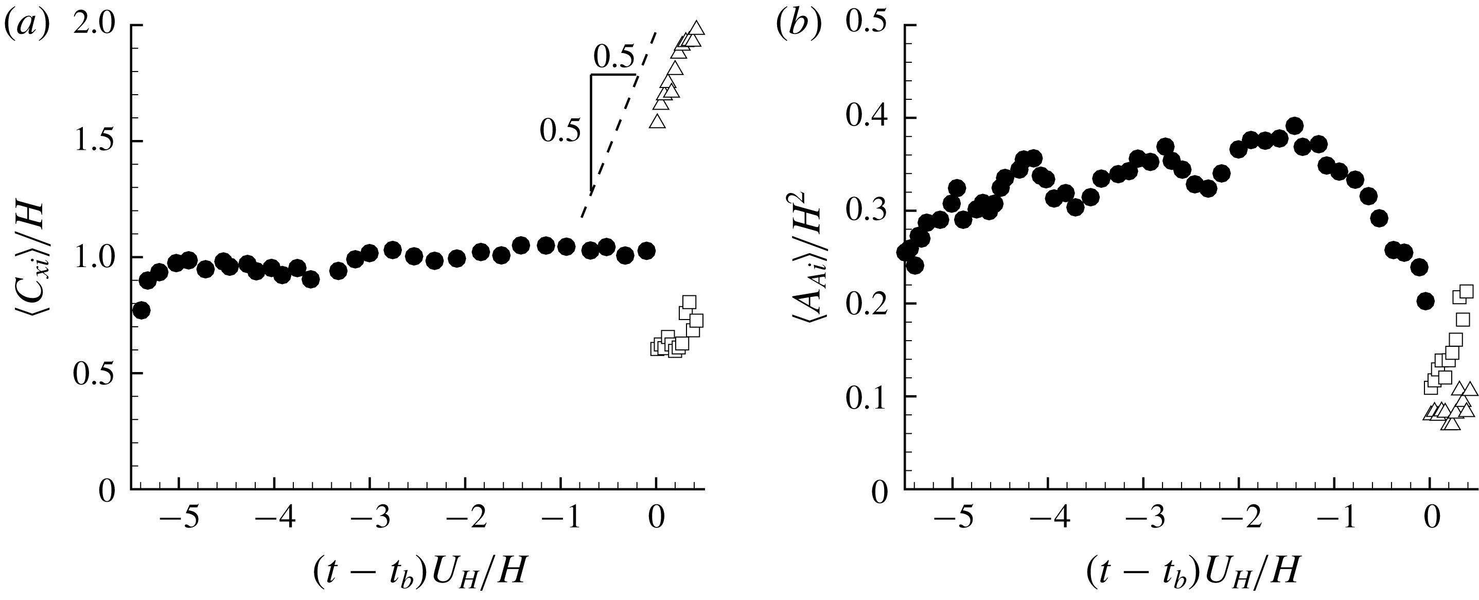
separating two concentrated areas (see coloured areas) of reverse flow. In other words, two separation bubbles occur at the particular instant shown in figure 16. To the best knowledge of the authors, the unsteady characteristics and the underlying physical mechanisms associated with SBBU events have not been reported in the existing literature.
Instantaneous areas of reverse flow. Solid isopleth is at
 $u=0$
. Areas in blue and red colours are two detected separation bubbles above the step, with the
 $x$
coordinates of centroids marked as
 $C_{x1}$
and
 $C_{x2}$
, respectively. The pre-defined minimal distance of different separation bubbles is marked as
 $d_{b}$
for reference.
In order to further study the SBBU events, a definitive/quantitative detection of multiple separation bubbles is needed. To this end, the following steps are performed for each snapshot:
- Step 1.
Grids of negative streamwise velocity
 $u$
are marked.
- Step 2.
Preliminary separation bubbles are identified by grouping all the connected (adjacent) grids of negative
$u$
.- Step 3.
Find the minimal distance of every two separation bubbles. If this distance is smaller than a predefined length
$d_{b}$
, combine these two separation bubbles into one separation bubble.- Step 4.
Repeat Step 3 until the number of separation bubbles does not change.


In figures 8(a) and 16, small areas of reverse flow can exist near the relatively larger concentrated areas of reverse flow. This can be caused by two-dimensional slicing (due to the planar PIV used in the present study) of irregular surfaces of three-dimensional volumes of reverse flow. The value of
 $d_{b}$
in Step 3 should not be too small or too large. Too small a value of
 $d_{b}$
(say
 $d_{b}=0$
) would exclude the possibility of capturing the irregular surfaces of three-dimensional volumes of reverse flow, while too large a value of
 $d_{b}$
would include too much distortion of small-scale randomness. An extremely large
 $d_{b}$
(say
 $d_{b}=2.3H$
) would group all areas of reverse flow above the step into one bubble and ignore the existence of multiple separation bubbles, which is equivalent to the approach used by Pearson et al. (Reference Pearson, Goulart and Ganapathisubramani2013). Here, we choose
 $d_{b}=0.065H$
(6 vector spacing), because it shows a reasonable balance between noise and genuine SBBU. We performed a sensitivity analysis by trying different values of
 $d_{b}$
: slightly earlier or delayed time of SBBU was predicted, however, minor differences in the conditionally averaged results were observed. We also choose to discard bubbles of reverse flow with less than 20 % of the maximum area. This is to further avoid the distortion from small bubbles. We have tried to use 10 % as the threshold but the results were not significantly altered, which would indicate that the small random bubbles of reverse flow are typically much smaller than the ‘genuine’ large-scale separation bubbles. With the procedures described above, the two areas of reverse flow are detected and marked in figure 16.
With the procedure described above to detect multiple separation bubbles, it is observed that the probabilities of one and two separation bubble(s) are 81.5 % and 15.2 %, respectively. It is only for 3.3 % of the time that more than two bubbles are detected, which could be caused by the imperfection of our detection approach or instances when the separation bubbles actually break into more than two pieces. In this paper, we choose to limit our attention to the cases with one or two separation bubbles. For convenience, the separation bubble closer to the leading edge is named as TSBA1, and that closer to the trailing edge is represented as TSBA2. Properties of TSBA1 and TSBA2 are denoted using subscripts of
 $(\cdot )_{1}$
and
 $(\cdot )_{2}$
, respectively. For example,
 $A_{A1}$
and
 $A_{A2}$
denote the areas of continuous reverse flow closer to the leading edge and trailing edge, respectively.
Time variation of (a) streamwise centroids and (b) areas of bubbles of reverse flow. Solid circles are for the single-bubble phase. Hollow squares and hollow triangles denote centroids or areas of reverse flow in TSBA1 and TSBA2, respectively. For clarity, every tenth measurement point is plotted here.
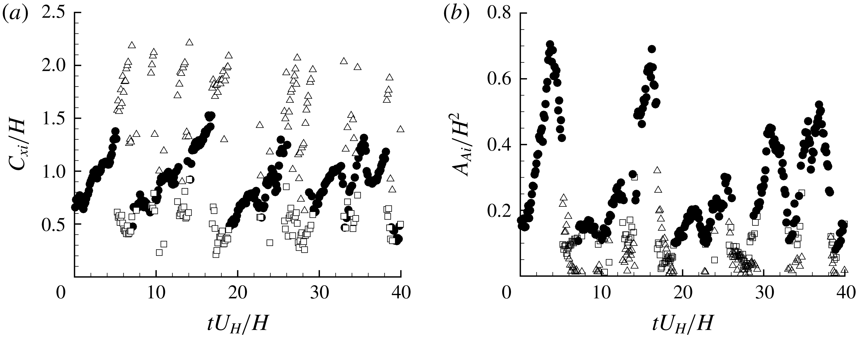
Premultiplied spectra of number of separation bubbles over the step.
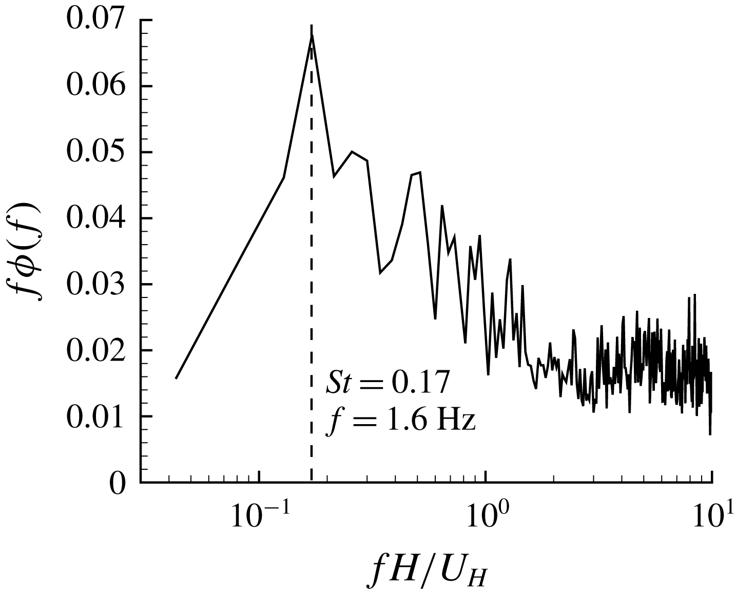
Figure 17 shows the sample time variation of streamwise centroids and areas of reverse flow. From the figures, the turbulent separation bubbles alternate between the single- and dual-bubble phases and show a quasi-periodic pattern. As shown in figure 18, the premultiplied spectrum of the number of bubbles of reverse flow possesses a sharp peak at the frequency
 $St=0.17$
.
Conditional averaged (a) streamwise centroids
 $\langle C_{xi}\rangle$
and (b) areas of reverse flow
 $\langle A_{Ai}\rangle$
during one period of SBBU. The single separation bubble breaks up at time
 $t=t_{b}$
. For clarity, every fourth point is plotted here. Refer to figure 17 for the legend.
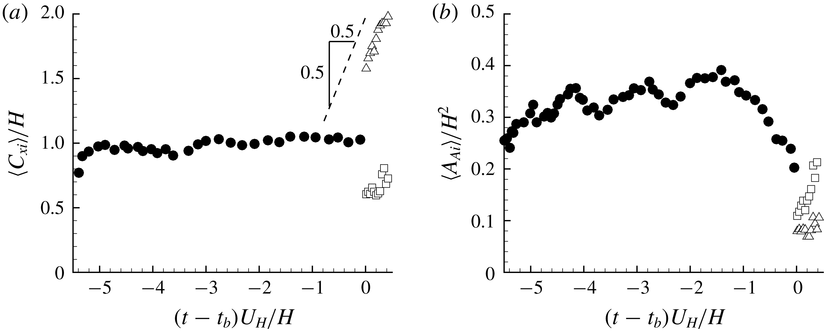
To provide further insight into the quasi-periodic breakup of the separation bubbles, we calculate the conditionally averaged areas and streamwise centroids of separation bubbles of reverse flow near SBBU events, and the results are shown in figure 19. For this analysis, the breakup event is fixed at
 $t=t_{b}$
, and the parameters (here
 $C_{xi}$
and
 $A_{Ai}$
) of separation bubbles in the adjacent time intervals are averaged until the last or next breakup event is reached (similar to (2.8) for the VITA approach). As such, figure 19 can be understood as an averaged evolution path of bubbles of reverse flow within a period of SBBU. In accordance with figure 18, the duration of each cycle of alternating single- and dual-bubble phases is
 $tU_{H}/H=1/0.17\approx 5.9$
. From figure 19, for the majority of the period of SBBU, the turbulent separation on top of the step is retained in the single-bubble phase, and the dual-bubble phase only occupies a very short time interval of the entire period. As seen in figure 19(b), right before the breakup events occur (
 $(t-t_{b})U_{H}/H\in [-1,0]$
), the area with a single bubble of reverse flow shrinks drastically. Furthermore, after the SBBU event, the area of the bubble of reverse flow closer to the leading edge (marked as hollow squares) clearly grows to that of the single bubble around
 $(t-t_{b})U_{H}/H=-5.5$
. In figure 19(a), the centroids of the bubbles of reverse flow closer to the trailing edge (marked as hollow triangles) vary linearly with time and the slope is almost exactly unity. With the observations in figures 19(a,b), we are able to describe the process within one period of SBBU event as follows. A large single turbulent separation bubble exists above the step, but somehow (as will be further explored in the next section) it shrinks rapidly in size, and eventually breaks up into two separation bubbles. After that, the separation bubble closer to the leading edge enlarges in size while the separation bubble closer to the trailing edge is convected downstream at a speed of
 $U_{H}$
. Eventually, the downstream separation bubble is convected farther away from the step, so that the separation bubble closer to the leading edge becomes the only separation bubble over the step, and the above cycle repeats.
3.6 POD analysis
In this section, POD is employed to extract the dominant coherent structures pertinent to the unsteadiness of TSBA. To this end, we choose to conduct the POD analysis in the region of
 $x/H\times y/H\in [0.04,2.24]\times [1.02,1.90]$
. The implementation and some necessary concepts/notations of POD have been introduced in § 2.3.3. Although not shown here, POD has been conducted with different sample sizes to perform a convergence test. The results indicate that a total of 32 000 samples is sufficient to ensure that the POD results are fully converged. Energy distributions amongst the first eighty modes and velocity fields of the first four modes are plotted in figures 20 and 21, respectively. The first four modes contribute
 $28.3\,\%$
,
 $9.4\,\%$
,
 $5.9\,\%$
and
 $3.7\,\%$
(
 $47.3\,\%$
in total), respectively, to the total TKE, indicating the dominance of these four modes, particularly the first two modes. The first four modes seem to exhibit a universal behaviour. Thacker et al. (Reference Thacker, Aubrun, Leroy and Devinant2013) performed POD for separation flow induced by an Ahmed body. Their first four modes contributed
 $28.0\,\%$
,
 $9.5\,\%$
,
 $6.0\,\%$
and
 $3.5\,\%$
, respectively, to the total TKE. Mohammed-Taifour & Weiss (Reference Mohammed-Taifour and Weiss2016) also conducted POD analysis for an adverse-pressure-gradient-induced turbulent separation flow. The percentages of the first four modes to the total TKE are
 $31\,\%$
,
 $9\,\%$
,
 $6\,\%$
and
 $4\,\%$
, respectively. In spite of significant differences in geometries and upstream conditions, Thacker et al. (Reference Thacker, Aubrun, Leroy and Devinant2013) and Mohammed-Taifour & Weiss (Reference Mohammed-Taifour and Weiss2016) showed similar energy convergence of the first four POD modes to ours. Furthermore, the four modes plotted in figure 21 are qualitatively similar to those in Thacker et al. (Reference Thacker, Aubrun, Leroy and Devinant2013) and Iftekhar & Agelin-Chaab (Reference Iftekhar and Agelin-Chaab2016) for different turbulent separations. The similarity between our POD modes and those of different geometries and upstream conditions indicates that POD is capable of capturing some universal features of turbulent separation bubbles.
Energy distributions among the first 80 POD modes.

The first four POD modes for the rectangular region of
 $x/H\in [0.04,2.24]$
and
 $y/H\in [1.02,1.90]$
. The superimposed solid and dashed isopleths are
 $\unicode[STIX]{x1D6F9}=0$
and
 $\unicode[STIX]{x1D6FE}=0.5$
, respectively. For clarity, every tenth vector is plotted.
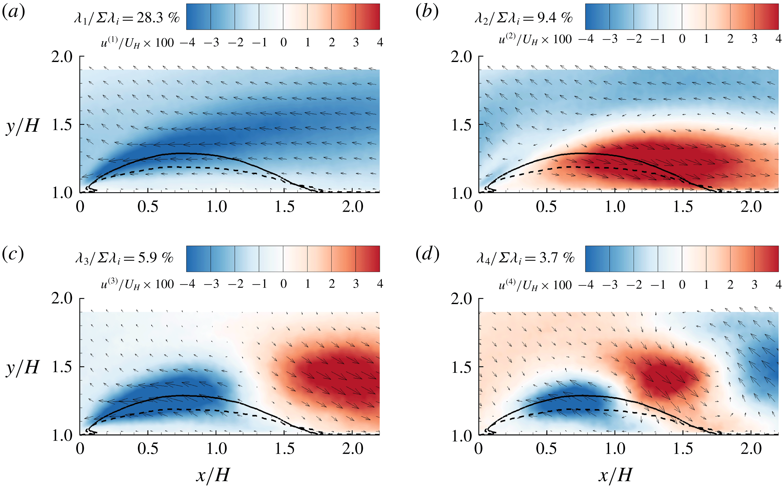
3.6.1 The first POD mode
In the literature, the first POD mode has been attributed to the low-frequency flapping motion of separations induced by a shock wave (Humble, Scarano & van Oudheusden Reference Humble, Scarano and van Oudheusden2009), geometry (Thacker et al.
Reference Thacker, Aubrun, Leroy and Devinant2013) and adverse pressure gradient (Mohammed-Taifour & Weiss Reference Mohammed-Taifour and Weiss2016). This interesting observation is further examined in our test case. Figure 22 compares the time sequences of the area of TSBA (
 $A_{A}$
) and the coefficients of the first mode (
 $a^{(1)}$
). The synchronization between these two temporal signals is remarkable. Furthermore, figure 23 shows that the premultiplied frequency spectrum of
 $a^{(1)}$
possesses a sharp peak at
 $St=0.070$
, almost identical to the dominant frequency (
 $St=0.075$
) of
 $A_{A}$
observed in figure 10(b). Based on the above observations, the dominant frequency of TSBA at
 $St=0.070$
is closely related to the first POD mode. Furthermore, as seen in figure 21(a), streamwise fluctuation of the first POD mode (
 $u^{(1)}$
) is of uniform sign over the entire mean separation bubble. Consequently, depending on the signs of its coefficient, the first POD mode represents a structure that can effectively enlarge or shrink the TBSA. Therefore, the dominant unsteady characteristic of TSBA revealed in figure 10(b) is a quasi-periodic enlargement/shrinkage flapping motion of turbulent separation at a low frequency of
 $St=0.075$
.
Time sequences of
 $a^{(1)}$
and
 $A_{A}$
.

Premultiplied frequency spectra (
 $f\unicode[STIX]{x1D719}^{(j)}(f)$
with
 $j=1$
or 2) of coefficients of the first two POD modes.
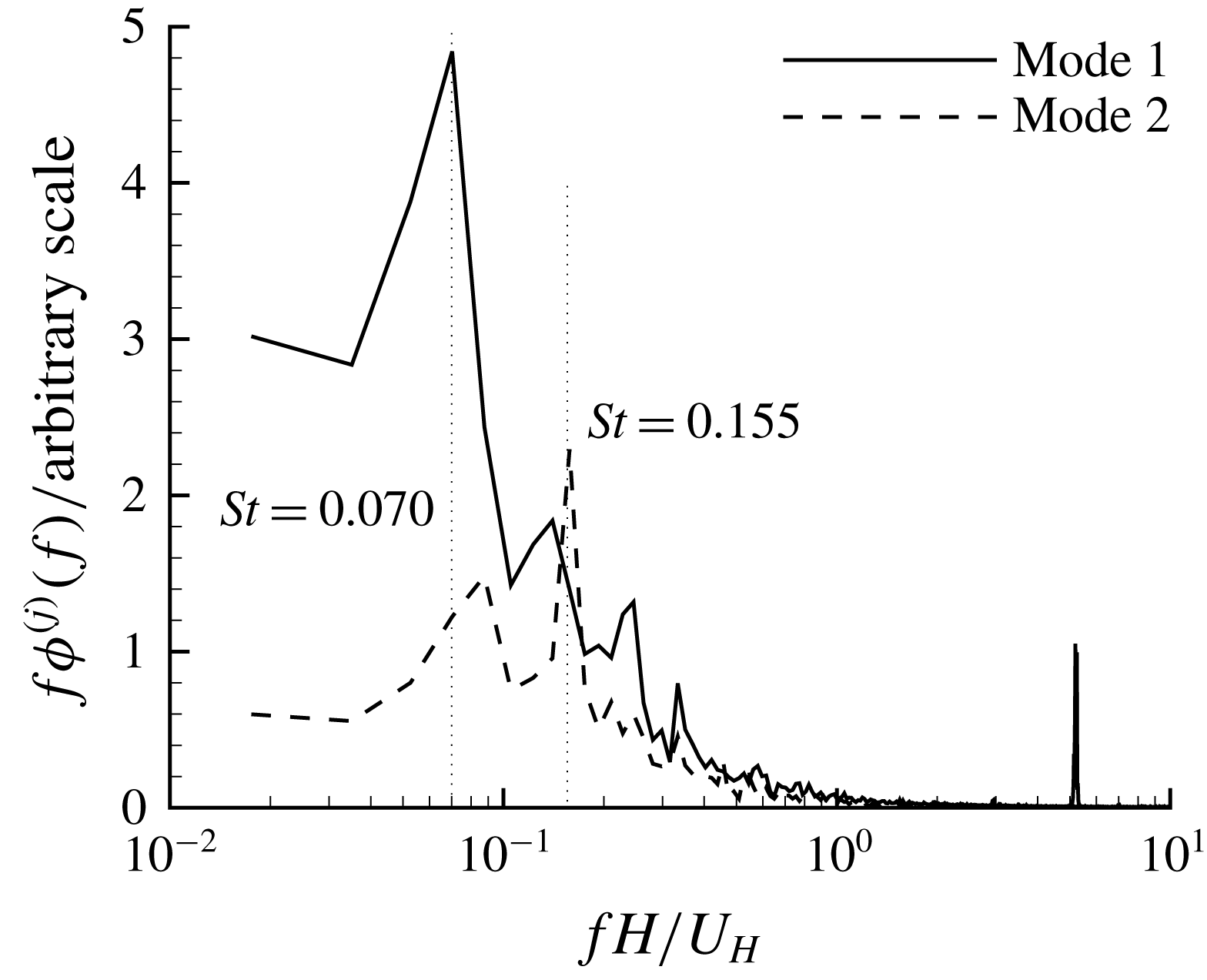
Probability density function (PDF) and cumulative density function (CDF) of
 $A_{A}$
. The mean value
 $\overline{A_{A}}/H^{2}$
is 0.29.
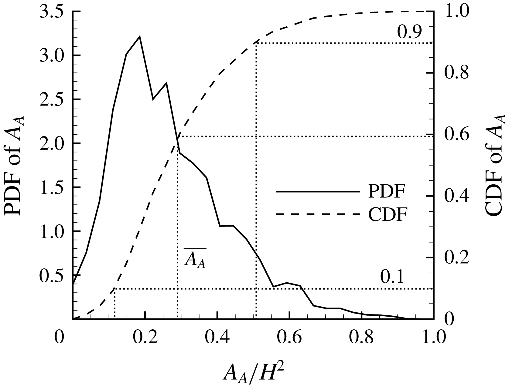
Conditionally averaged streamlines (shown as green streamlines) and velocity fluctuations (shown as vectors) based on different sizes of
 $A_{A}$
: (a)
 $A_{A}/H^{2}\in [0.037,0.074]$
and (b)
 $A_{A}/H^{2}\in [0.482,0.519]$
. Note that the contour levels are different in these two panels. For clarity, every tenth vector is plotted.

In addition to the analysis based on the first POD mode, we also investigate structures associated with different sized TSBA from a different perspective. Figure 24 shows the probability density function (PDF) and cumulative density function (CDF) of
 $A_{A}$
. It is interesting to see that the PDF of
 $A_{A}$
does not decay to zero at
 $A_{A}=0$
. This raises the possibility that turbulent flow over the step is completely (at least to the measurement accuracy) attached to the top surface. Furthermore, as indicated by the right tail of the PDF,
 $A_{A}$
can be even larger than
 $2\overline{A_{A}}$
. Figure 25 shows the conditionally averaged streamlines and velocity fluctuation fields, based on the conditions of specified ranges of
 $A_{A}$
. As such, figure 25(a,b) represents the scenarios of shrinkage and enlargement of TSBA, respectively. The patterns of the conditionally averaged fluctuating velocity fields (represented by vectors) in figure 25(a,b) are qualitatively similar to the first POD mode shown in figure 21(a), albeit different in sign. This is consistent with our previous discussion that low-frequency flapping motion of TSBA reflects periodic enlargement/shrinkage of the separation bubble, and is intimately associated with the first POD mode.
As seen in figure 21(a), negatively valued
 $a^{(1)}$
(coefficient of the first POD mode) most likely occurs in instances when the TSBA shrinks, and pronounced sweep (
 $Q4$
featuring
 $u^{\prime }>0$
and
 $v^{\prime }<0$
) events in the region above and upstream (see the top-left corner area) of the mean separation bubble. This is consistent with the conditionally averaged fluctuating velocity field shown in figure 25(a). With the same logic, positively valued
 $a^{(1)}$
leads to
 $Q2$
events in the upstream location of TSBA, which is also consistent with observation in figure 25(b). Overall, the shrinkage and enlargement of TSBA are also accompanied by upstream
 $Q4$
and
 $Q2$
events, respectively. This important conclusion is also consistent with the observation that the flapping motion of the TSBA occurs at a frequency (
 $St=0.075$
) very close to the dominant frequency of the upstream streamwise velocity fluctuation (see figures 15
b and 10
b).
In the literature, there is a debate on the mechanism of the flapping motion of TSB. Ganapathisubramani, Longmire & Marusic (Reference Ganapathisubramani, Longmire and Marusic2003), Ganapathisubramani, Clemens & Dolling (Reference Ganapathisubramani, Clemens and Dolling2007, Reference Ganapathisubramani, Clemens and Dolling2009) attributed the low-frequency unsteadiness of a shock-induced TSB to the oncoming elongated superstructures, which feature alternating positive and negative
 $u^{\prime }$
(Adrian et al.
Reference Adrian, Meinhart and Tomkins2000). Similarly, Pearson et al. (Reference Pearson, Goulart and Ganapathisubramani2013) linked the enlargement of TSB in front of an FFS to oncoming low-velocity regions elongated in the streamwise direction by
 $2\unicode[STIX]{x1D6FF}$
to
 $12\unicode[STIX]{x1D6FF}$
. For their adverse-pressure-gradient-induced TSB, Mohammed-Taifour & Weiss (Reference Mohammed-Taifour and Weiss2016) remarked that their observed characteristic frequencies are ‘smaller than the high-frequency turbulent fluctuation’, and therefore void the possibility of oncoming elongated superstructure causing the flapping motion of TSB. They proposed two possible mechanisms to explain the low-frequency flapping motion: side wall effects and inherent unsteadiness of the TSB. These two mechanisms are not applicable in our case. The aspect ratio of the TSB (ratio between spanwise width and TSB height) in Mohammed-Taifour & Weiss (Reference Mohammed-Taifour and Weiss2016) was approximately 6, whereas that in our case is more than 100 (our TSB height is lower than 0.2
 $H$
in figure 4, and the spanwise width of the step is 20
 $H$
). Therefore, it is highly unlikely that our
 $x$
–
 $y$
plane measurement in the channel centre is affected by side walls.
It should be noted that although superstructures populated in the log region of the TBL can extend up to
 $20\unicode[STIX]{x1D6FF}$
in the streamwise direction, their strong meandering nature significantly shortens their characteristic length scales inferred from premultiplied energy spectra or two-point correlations (Hutchins & Marusic Reference Hutchins and Marusic2007). Since PIV measurement in the streamwise–vertical plane cannot capture the spanwise-meandering nature of superstructures, it is more reasonable to reference the characteristic length scales of TBL deduced from energy spectra or two-point correlations in the literature for comparison. Adrian et al. (Reference Adrian, Meinhart and Tomkins2000), Ganapathisubramani et al. (Reference Ganapathisubramani, Longmire and Marusic2003), Tomkins & Adrian (Reference Tomkins and Adrian2003), Ganapathisubramani et al. (Reference Ganapathisubramani, Hutchins, Hambleton, Longmire and Marusic2005) and Monty et al. (Reference Monty, Hutchins, Ng, Marusic and Chong2009) concluded that streamwise-elongated low-velocity regions are surrounded by packets of vortical structures, and can extend between
 $2\unicode[STIX]{x1D6FF}$
and
 $3\unicode[STIX]{x1D6FF}$
in length. Assuming the convective velocity in the TBL is approximately 0.8
 $U_{\infty }$
, the associated frequency of these streamwise-elongated structure is estimated to be
 $St=0.08{-}0.12$
. This estimation is consistent with the observation from figure 15(b) that the streamwise fluctuation in the upstream TBL possesses a peak frequency around
 $St=0.075$
(see the dotted vertical line). Moreover, this dominant frequency (
 $St=0.075$
) is also close to the frequency of flapping motion observed in figures 10(b) and 23, i.e.
 $St=0.070{-}0.075$
. It is further noted that the frequency of the flapping motion of TSBA is quite different to the separation over a blunt body with a laminar upstream condition. With a uniform upstream condition, Kiya & Sasaki (Reference Kiya and Sasaki1983) measured the enlargement/shrinkage of a bubble over a blunt body to be at a frequency of
 $0.2U_{\infty }/x_{R}$
(where
 $x_{R}$
denotes the reattachment length). In contrast, the frequency of flapping motion observed in the present study (
 $St=0.075$
) corresponds to a much (more than 30 times) larger value of
 $6.1U_{\infty }/x_{R}$
. This indicates that the upstream perturbation overcomes the intrinsic frequency of TSBA. Furthermore, by using the POD analysis and conditional averaging, it is observed that the enlarged and shrunken TSBA is related to low- and high-velocity regions covering the entire area of the mean separation bubble. Thus, we concluded that the low-frequency flapping motion of TSBA is due to oncoming streamwise-elongated regions of alternating positive and negative streamwise-fluctuating velocity.
VITA fluctuation of the area of reverse flow in TSBA (
 $A_{A}^{\prime }$
), coefficient of mode 1 (
 $a^{(1)}$
) and upstream
 $u^{\prime }$
at
 $(x/H,y/H)=(-2.3,1.1)$
. Note that VITA of
 $A_{A}^{\prime }$
and
 $a^{(1)}$
are inverted to facilitate the comparison with VITA of
 $u^{\prime }$
. Also note that all signals are pre-filtered to remove insignificant (trivial energy levels) fluctuations at very high frequencies.
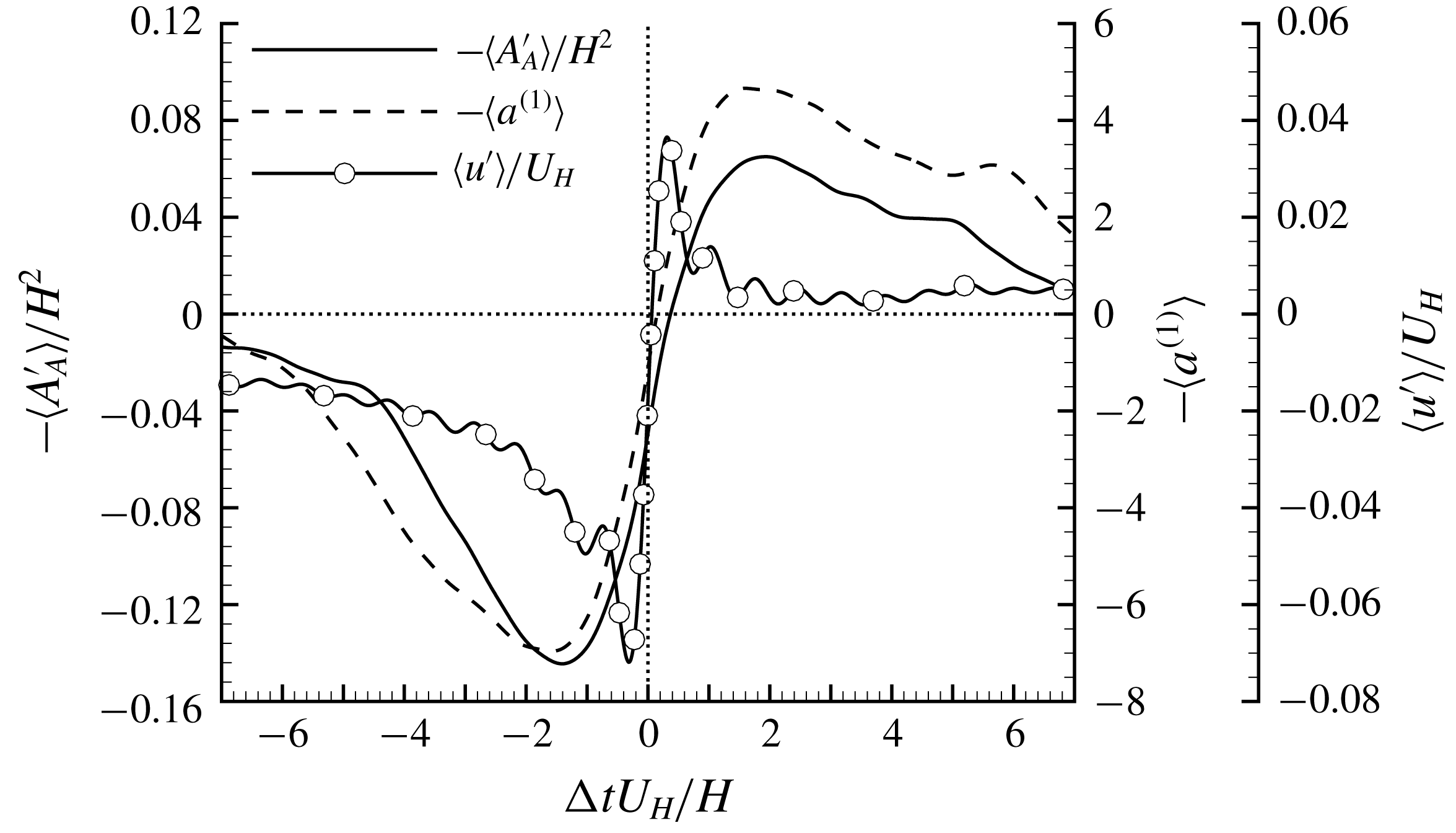
With the above analysis, it is intuitive to imagine the step as a ‘probe’ in a TBL and the size of TBSA is a direct measurement of the oncoming turbulence structures. Specifically, an enlarged and shrunken TBSA would indicate upstream
 $Q2$
and
 $Q4$
events, respectively. Inspired by this analogy, it is of interest to further examine TBSA in terms of probe-like characteristics. A straightforward and (probably the most) appropriate examination is one based on the VITA events of TBL. VITA was originally proposed by Blackwelder & Kaplan (Reference Blackwelder and Kaplan1976) as a conditional averaging technique for temporal signals acquired using hot-wires in TBL. Since then, VITA has been primarily used to detect the sudden switching between
 $Q2$
and
 $Q4$
events (or turbulent burst events), which is now commonly termed a VITA event (Adrian et al.
Reference Adrian, Meinhart and Tomkins2000). It is now generally accepted that a VITA event occurs when a hairpin vortex structure passes a probe, a
 $Q2$
event suddenly switches to a
 $Q4$
event near the stagnation line below the hairpin head (Adrian et al.
Reference Adrian, Meinhart and Tomkins2000) (also see figure 3).
The VITA technique is applied to three temporal signals:
 $-A_{A}^{\prime }$
,
 $-a^{(1)}$
and upstream
 $u^{\prime }$
at (
 $x/H$
,
 $y/H$
)
 $=$
(
 $-2.3$
, 1.1), and the results are shown in figure 26. In the figure, note the negative signs for
 $-A_{A}^{\prime }$
and
 $-a^{(1)}$
; this is because
 $\text{d}(-A_{A}^{\prime })/\text{d}t>0$
and
 $\text{d}(-a^{(1)})/\text{d}t>0$
are associated with the switching from
 $Q2$
to
 $Q4$
events, and so is
 $\text{d}u^{\prime }/\text{d}t>0$
. A low-pass filter is pre-applied to the signals to remove spurious fluctuations associated with
 $St>1.5$
because only the low-frequency signal around
 $St=0.075$
is of primary interest. In figure 26, the signal is averaged over
 $\unicode[STIX]{x0394}tU_{H}/H\in [-7,7]$
, a time interval associated with the period of
 $St=0.075$
, to visualize the variation during the period of the dominant frequency. The parameter
 $T$
in (2.7) was varied from
 $3.5H/U_{H}$
to
 $0.7H/U_{H}$
, and the results were not significantly affected. The results shown in figure 26 are from
 $T=0.7H/U_{H}$
in (2.7).
From figure 26, the variations of
 $-\langle A_{A}^{\prime }\rangle$
and
 $-\langle a^{(1)}\rangle$
with
 $\unicode[STIX]{x0394}t$
are similar (e.g. they both peak around the same
 $\unicode[STIX]{x0394}t$
and possess similar slopes around event points). This again suggests a direct connection between areas of TSBA and the first POD mode. Furthermore, the localized strong events (quantified by the variance of (2.7)) of TSBA is evidently associated with a swift shrinkage of the separation bubble, as indicated by the observation that
 $-\langle A_{A}^{\prime }\rangle$
changes from negative (corresponding to larger TSBA) to positive (corresponding to smaller TSBA) values very quickly around VITA events (
 $\unicode[STIX]{x0394}t=0$
). As indicated by
 $-\langle a^{(1)}\rangle$
, the swift shrinkage of TSB is associated with a sudden switching from
 $Q2$
to
 $Q4$
events in the upstream condition. It is also seen that the slope of
 $\langle u^{\prime }\rangle$
around event point (
 $\unicode[STIX]{x0394}t=0$
) is apparently steeper than that of
 $-\langle A_{A}^{\prime }\rangle$
and
 $-\langle a^{(1)}\rangle$
. This can be explained as follows:
 $\langle u^{\prime }\rangle$
is a point-wise measurement and can respond (switch from
 $Q2$
to
 $Q4$
events) immediately as the stagnation line shown figure 3 passes the reference point. In contrast, both
 $-\langle A_{A}^{\prime }\rangle$
and
 $-\langle a^{(1)}\rangle$
represent measurements over a finite area, therefore, it takes a relatively longer time for the flow in the conditioned area to respond. Overall, TSBA indeed shows a probe-like behaviour: its enlargement and shrinkage are intimately related to the upstream
 $Q2$
and
 $Q4$
events, respectively, albeit with a lag during switching.
Conditionally averaged streamlines and streamwise-fluctuating velocity based on the condition of
 $C_{x2}/H\in [1.47,1.56]$
. Time is shifted by
 $\unicode[STIX]{x0394}tU_{H}/H=$
(a)
 $-0.38$
, (b)
 $-0.19$
, (c) 0.00 and (d)
 $+0.19$
, respectively.
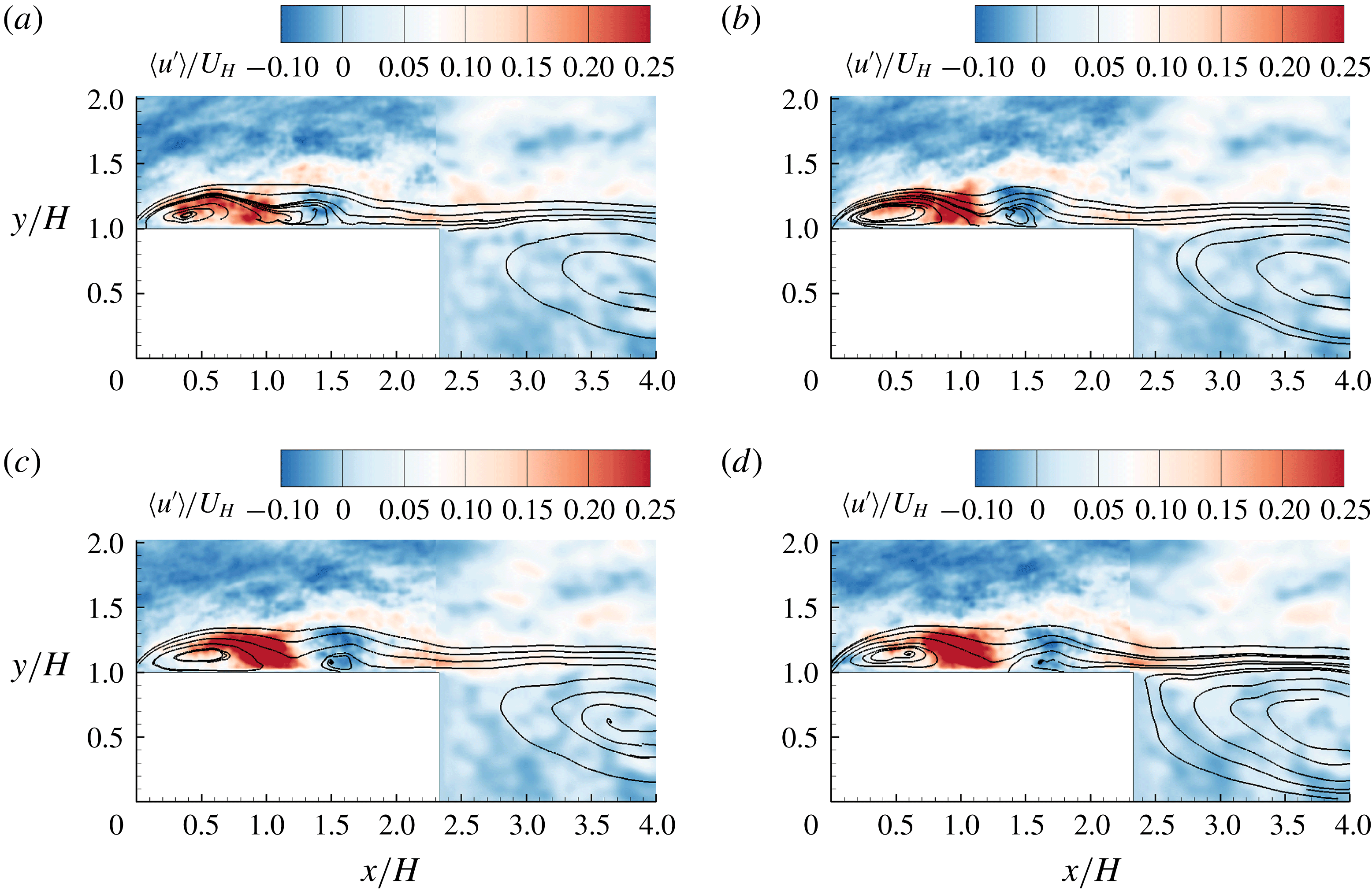
3.6.2 The second POD mode
From figure 23, the second POD mode possesses a dominant frequency at
 $St=0.155$
. This frequency is close to the subdominant frequency (
 $St=0.141$
) of TSBA observed in figure 10(b) and the dominant frequency (
 $St=0.17$
) of SBBU observed in figure 18. This interesting observation prompts us to further examine the possibility of intimate connections between SBBU events and the second POD mode. To this end, conditionally averaged flow fields are calculated based on the condition of
 $C_{x2}/H\in [1.47,1.56]$
, as shown in figure 27(c). This particular range of
 $C_{x2}/H$
is chosen here because it is close to the averaged position of the second separation bubble near the breakup event (see figure 19
a). The samples for the conditional average in figure 27(c) are further shifted by different time intervals, and plotted in figure 27 to illustrate a typical evolution of an SBBU event. From the conditionally averaged streamlines shown in figure 27(c), it is clear that two separation bubbles exist, as imposed by the averaging condition. This also demonstrates the effectiveness of the proposed procedure to identify multiple separation bubbles in § 3.5. In figure 27(a), a single separation bubble is evident, and is apparently squeezed by an area of positive
 $u^{\prime }$
around separating streamlines. This is consistent with the observation in figure 19(b) that prior to the SBBU event, the area of a single separation bubble shrinks. As time shifts to figure 27(b), two separation bubbles are detached from each other, and the positive
 $u^{\prime }$
along separating streamlines is enhanced. As time further evolves from figures 27(b) to 27(d), the second separation bubble is convected towards the trailing edge. This is consistent with the observation in figure 19(a) that the second separation bubble moves towards the trailing edge after formation.
It is also interesting to see in figure 27 that the sudden appearance of strong positive
 $u^{\prime }$
over the step is associated with negative
 $u^{\prime }$
in the upstream location. This pattern is qualitatively similar to the second POD mode shown in figure 21(b). Furthermore, in accordance with the observation that the second POD mode (figure 23) and SBBU (figure 18) both possess a dominant frequency around the subdominant peak of TSBA (figure 10
b) around
 $St=0.14{-}0.17$
, we conclude that the second POD mode is indeed linked to the SBBU events.
From figure 21(a), the largest magnitudes of
 $u^{\prime }$
in the first POD mode occur in an area emanating from the leading edge. This pattern is consistent with the distribution of Reynolds stress
 $\overline{u^{\prime }u^{\prime }}$
shown in figure 6(a), reflecting the dominance of the first POD mode. In contrast, the second POD mode possesses weak
 $u^{\prime }$
closer to the leading edge, but exhibits strong
 $u^{\prime }$
in an area along separating streamlines in the rear part of TSBA. This pattern is very similar to the distribution of
 $\overline{u^{\prime }u^{\prime }}$
over an FFS with an upstream laminar flow (Kiya & Sasaki Reference Kiya and Sasaki1983; Djilali & Gartshore Reference Djilali and Gartshore1991), and the most unstable mode of a separation bubble over an FFS predicted by linear stability analysis (Alam & Sandham Reference Alam and Sandham2000; Lanzerstorfer & Kuhlmann Reference Lanzerstorfer and Kuhlmann2012). Yang & Voke (Reference Yang and Voke2001) studied the transition of separation bubble over a blunt body with an upstream uniform flow, and also showed that large (comparable to the mean separation bubble) circular bubbles may form and shed downstream, which is similar to the observation in figure 27. Based on these analyses, we further conclude that the second POD mode and SBBU events indeed reflect the intrinsic instability of TSBA itself.
Lanzerstorfer & Kuhlmann (Reference Lanzerstorfer and Kuhlmann2012) shows that production of TKE in the region along separating streamlines in the rear part of separation bubble is mostly due to the classical lift-up process by streamwise-elongated counter-rotating vortices (SCV) (Zhou et al. Reference Zhou, Adrian, Balachandar and Kendall1999). On the other hand, it is commonly accepted that low-velocity region in TBL is induced by packets of hairpin structures, also featuring SCV in the near-wall region (Adrian et al. Reference Adrian, Meinhart and Tomkins2000). For the current deep TBL, it is expected that SCV from the oncoming TBL at an elevation higher than the step height is quite popular. As such, SCV from the oncoming TBL can easily trigger SCV associated with the unstable mode of separation bubble over the step. This analysis is also compatible with the idealized model of hairpin packets (Zhou et al. Reference Zhou, Adrian, Balachandar and Kendall1999; Adrian et al. Reference Adrian, Meinhart and Tomkins2000), as explained in the following. In hairpin packets, multiple hairpin structures align in the streamwise direction and generate elongated zones of nearly uniform low streamwise velocity. As hairpin packets pass the step, the separation bubble becomes larger due to a momentum deficit induced by low-velocity streaks, and breaks up as discrete hairpin structure triggers the inherent unstable mode. This also explains the reason why the flapping motion occurs at a lower frequency than the separation bubble breakup.
With the above analyses, the SBBU event is a manifestation of the intrinsic instability near the rear part of TSBA, even with the upstream turbulent flow condition. This is not surprising. Marquillie, Laval & Dolganov (Reference Marquillie, Laval and Dolganov2008) performed a DNS investigation for a turbulent plane channel flow with a smooth bump on the bottom wall. They observed that vortical structures were more clustered in the rear part of the separation bubble. In their follow-up research using a linear stability analysis, Marquillie, Ehrenstein & Laval (Reference Marquillie, Ehrenstein and Laval2011) further showed that streamwise-elongated streaky structures could induce hairpin-type structures in the rear part of the separation bubble. The current observed SBBU event can be a manifestation of energetic vortical structures generated near the reattachment point moving downstream. This is similar to the observation by Na & Moin (Reference Na and Moin1998) in a TBL separated due to an adverse pressure gradient that in the shear layer bounding the separation bubble, vortical structures grew, agglomerated and then convected downstream.
The superposition of low-frequency flapping motion and high-frequency unstable mode of TSBA described above may also explain the destruction mechanism of streamwise coherence near the leading edge deduced from figure 14(e,f). The first POD mode (equivalently, the flapping motion) tends to correlate (quantified by positively valued
 $R_{uu}$
)
 $u^{\prime }$
over the step with that in front of the leading edge. However, the SBBU event (see figures 21(b) and 27) of TSBA features a pattern where
 $u^{\prime }$
switches signs along a boundary emanating from the leading edge of the step. This pattern tends to cause negatively valued
 $R_{uu}$
over the step with the reference point fixed in front of the leading edge, and vice versa. Therefore, the superposition of the first two POD modes can lead to a very weak correlation (
 $R_{uu}$
) between structures upstream and downstream of the leading edge, as shown in figure 14(e,f).
4 Conclusions
Turbulent separations over a forward–backward-facing step were investigated using a time-resolved particle image velocimetry system. The thickness of the upstream turbulent boundary layer is significantly larger than the step height. This induces strong interactions between upstream vortical structures with the step. The streamwise extent of the step was chosen to be large enough to allow reattachment of the mean flow over the step, yet small enough to permit interactions between turbulent separation bubble on top of the step and that behind the step, which are denoted as TSBA and TSBB, respectively.
The shear layers emanating from the leading and trailing edges of the step merge into a single shear layer at a distance sufficiently behind the step (
 $x/H>3.5$
). The strongest turbulent levels appear near the leading edge of the step, and decay in the downstream direction. This observation is in sharp contrast to previous experimental investigations of a separation bubble with laminar upstream conditions, where transition to turbulence occurs only in the rear part of the separation bubble. Furthermore, due to misalignment between the predefined streamwise direction and local mean streamlines, a strong positively valued Reynolds shear stress (i.e.
 $\overline{u^{\prime }v^{\prime }}>0$
) appears near the leading edge, which is at variance with the Boussinesq eddy-viscosity assumption. However, with the curvilinear coordinate system along mean streamlines, there exist regions inside or above the mean separation bubble within which the signs of the transformed Reynolds shear stress and mean strain rate are the same and therefore exhibit inconsistency with the Prandtl’s mixing-length hypothesis.
Through a spectral analysis, it is revealed that TSBA exhibits a low-frequency flapping motion at
 $St=0.075$
, featuring a quasi-periodic enlargement/shrinkage of separation bubble. Moreover, the dominant frequency of TSBB is at an even lower frequency of
 $St\approx 0.03$
, and a subdominant frequency of TSBB is induced by the interaction between TSBA and TSBB. Essentially, TSBB mirrors the same flapping motion of TSBA at the same frequency (
 $St=0.075$
), but with a distinct time delay of
 $7.6H/U_{H}$
.
Measurements in the streamwise–spanwise planes indicate that the spillover (vertical enlargement of separation bubble in front of the step) of reverse flow from the front of the step is typically associated with a pair of vertical counter-rotating vortices, and a streamwise-elongated low-velocity streak extending in the upstream direction. This confirms and clarifies the speculation by Pearson et al. (Reference Pearson, Goulart and Ganapathisubramani2013) that the enlargement and shrinkage of a separation bubble in front of an FFS is related to the transverse flow motion, which is influenced by upstream turbulence structures. Furthermore, there exists a strong destruction mechanism near the leading edge which in turn severely reduces the upstream streamwise coherence (quantified by two-point autocorrelation) to be extended over the step. This destruction mechanism is identified as the intrinsic unstable mode of TSBA.
The dominant structures underlying the unsteady characteristics of TSBA are further studied using proper orthogonal decomposition (POD) and various conditional averaging techniques. The results indicate that the first and second POD modes are associated with low-frequency flapping motion and higher-frequency inherent instability of TSBA, respectively. Meanwhile, the flapping motion of TSBA is associated with the enlargement and shrinkage of the separation bubble induced by oncoming elongated regions with a negative and positive streamwise-fluctuating velocity, respectively. The inherent instability of TSBA is accompanied by the sudden occurrence of an area of strong positive streamwise-fluctuating velocity over the step, and leads to separation bubble breakup. As two separation bubbles appear over the step, the separation bubble closer to the trailing edge of the step is convected downstream at a velocity of
 $U_{H}$
.
Acknowledgements
The financial support from Natural Sciences and Engineering Research Council (NSERC) of Canada and Canada Foundation for Innovation (CFI) is gratefully acknowledged. We would like to thank A. Nematollahi for his help in setting up the first few sets of experiments.