4.1 Parameters-Predictor application

This application is designed to forecast tracking parameters essential for satellite data acquisition, including azimuth (Az), elevation (El), and Doppler shift [Reference Bensikaddour, Nasri and Hamed31], alongside determining the optimal polarisation (LHCP or RHCP). As illustrated in Fig. 2, the application comprises various modules with distinct inputs and outputs, orchestrating a cohesive prediction framework.

Figure 2.

Different modules, inputs and outputs of Parameters-Predictor application.

Tracking parameters are calculated using the PyEphem library [Reference Rhodes32], a well-established tool for astronomical computations known for its reliability and ease of use. Predicting these parameters necessitates two inputs: TLE (two-line elements) files, which encapsulate standardised orbital parameters of objects orbiting the Earth, and GS coordinates, comprising latitude, longitude and altitude data. This module is thoroughly described in previous work [Reference Bensikaddour, Nasri and Hamed31]. Additionally, Parameters-Predictor incorporates trained machine learning models to predict signal power level in dBm for RHCP and LHCP polarisations.

4.1.1 Dataset and model training

It is well established that azimuth and elevation directly influence the quality of RHCP and LHCP signals due to their impact on the geometric alignment between the satellite and the GS [Reference Lighari, Berg, Kallankari, Parssinen and Salonen33]. These parameters can lead to variations due to phenomena such as diffraction, reflection or attenuation of electromagnetic waves. Therefore, these two parameters were chosen to build a model capable of predicting the signal power in both RHCP and LHCP polarisations.

The ALSAT-2 satellites’ GS (S-band) operates using programme tracking rather than autotrack. In this mode, azimuth and elevation parameters are predicted before the satellite pass and used to control the antenna in real time. While minor errors may occur due to control loop limitations (e.g. latency or mechanical constraints), these errors remain minimal and do not significantly affect tracking accuracy. It is important to note that the azimuth and elevation values used in the dataset correspond to the predicted values rather than real-time measured values.

The dataset used for model training consists of historical measurements obtained from the Alsat-2A and Alsat-2B satellites. These measurements include azimuth, elevation and power level data for both RHCP and LHCP polarisations. The data was leveraged to train ML models aimed at predicting signal power level. The dataset used for training the model consists of TM data from the Alsat-2A and Alsat-2B satellites. It includes azimuth, elevation and signal strength measurements for RHCP and LHCP polarisations, collected during satellite passes over 2022 and 2023 with a recording interval of 5 seconds. A total of 145,000 entries were extracted for each satellite. The data, converted to comma-separated values (CSV) format, were cleaned and preprocessed to address anomalies and missing values. These prepared datasets were used to train ML models to predict signal strength based on azimuth and elevation.

To evaluate model performance, the dataset was divided into two subsets:

• • Training set (80%) – used to train the machine learning model.

• • Test set (20%) – used to assess the model’s generalisation performance.

To enhance robustness and reduce bias, five-fold cross-validation was employed. The training set was divided into five folds, with four used for training and one for validation in each iteration. This process was repeated five times, ensuring that every data point was utilised for both training and validation.

In our study, missing data and anomalies occur in the signal power measurements for RHCP and LHCP, which are provided by the previous demodulator. These inconsistencies arise due to reception conditions (e.g. atmospheric disturbances) or temporary signal loss during low-power periods. Importantly, the azimuth and elevation values, which are predicted based on orbital data and used for antenna control, remain unaffected by these signal power level anomalies.

During data preprocessing, missing signal power level values were removed rather than interpolated, as interpolation could introduce artificial trends or inaccuracies. Anomalies, such as abrupt fluctuations in power levels, were identified and filtered using the interquartile range (IQR) method, which effectively detects extreme deviations that do not reflect normal signal behaviour. Since these anomalies account for only a small fraction (approximately 2%) of the dataset, and are concentrated in periods of low signal power (specifically below −55 dBm), their impact on the overall data distribution is minimal.

To further validate their minimal effect, we assessed the model’s performance before and after anomaly removal. The results showed no significant deviation in predictive accuracy, confirming that the anomalies were either negligible or inherently accounted for by the model’s learning process.

In Figs 3 and 4, the temporal evolution of the RF signal power level for RHCP and LHCP polarisations, and the variation of this power with respect to azimuth and elevation during a previous pass, are illustrated, respectively. Both subtle fluctuations and significant variations in signal power are displayed in these graphs. It is critical to note that the CDM 600 demodulator stops working when the signal power level drops to −60 dB or below, which could impact data acquisition.

Figure 3.

Temporal evolution of signal power level in RHCP and LHCP for a previous ALSAT-2A pass.

Figure 4.

Signal power level variation on RHCP and LHCP vs Az and El for a previous ALSAT-2A pass.

Two well-established ML algorithms, k-nearest neighbours (kNN) and random forest (RF), have been selected for this task. The selection of these algorithms was predicated on their robustness and proven track record in handling complex datasets [Reference Rhys34]. To fine-tune the parameters of these algorithms, automatic adjustments were executed using a Python script [Reference Random Forest35, 36]. Table 1 presents the optimised parameters for both algorithms as applied to the two satellites, Alsat-2A and Alsat-2B.

Table 1.

Tuning kNN and RF

To mitigate noise present in the training measurements, smoothing has been applied to the predicted values of RHCP and LHCP using a moving average. This technique helps in reducing noise and stabilising the predictions.

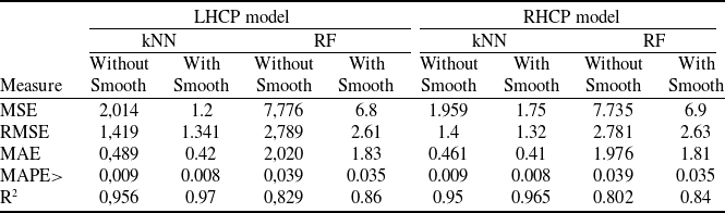
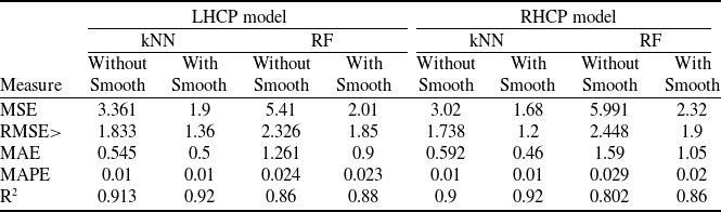
Tables 2 and 3 present the performance of the kNN and RF algorithms (without smoothing and with smoothing), evaluated using various metrics for ALSAT-2A and ALSAT-2B, respectively. The test set used for evaluation was derived from the same dataset as the training set but was kept separate to ensure an unbiased assessment of the model’s generalisation performance.

Table 2.

Performance of kNN and RF, using several evaluation metrics (ALSAT-2A)

Table 3.

Performance of kNN and RF, using several evaluation metrics (ALSAT-2B)

The smoothing was performed using a moving average with a window size of 8, selected based on empirical analysis and preliminary testing.

For the ALSAT-2A dataset, kNN consistently outperforms RF across all evaluation metrics for both LHCP and RHCP models. In the LHCP case, kNN has lower errors, with an MSE of 2.014 compared to 7.776 for RF. The RMSE (1.419 vs. 2.789), MAE (0.489 vs. 2.020), and MAPE (0.009 vs. 0.039) also show that kNN predictions are more accurate. The R² value of 0.956 for kNN confirms that it explains more of the signal’s variability compared to RF (R² = 0.829).

For the RHCP model in ALSAT-2A, the trend is the same. kNN achieves lower MSE (1.959 vs. 7.735), RMSE (1.4 vs. 2.781), MAE (0.461 vs. 1.976) and MAPE (0.009 vs. 0.039), showing better accuracy. Its R² value of 0.950 is also higher than RF’s 0.802.

For ALSAT-2B (Table 3), similar results are observed. In the LHCP case, kNN again performs better, with an MSE of 3.361 compared to 5.410 for RF. The RMSE (1.833 vs. 2.326), MAE (0.545 vs. 1.261) and MAPE (0.01 vs. 0.024) are all lower for kNN. The R² value of 0.913 for kNN confirms its better fit compared to RF (R² = 0.860).

For the RHCP model in ALSAT-2B, kNN remains superior. Its MSE (3.020 vs. 5.991), RMSE (1.738 vs. 2.448), MAE (0.592 vs. 1.590) and MAPE (0.01 vs. 0.029) are all smaller. The R² value for kNN (0.900) is also higher than for RF (0.802).

Overall, kNN consistently outperforms RF for both LHCP and RHCP models on ALSAT-2A and ALSAT-2B. This shows that kNN is better suited for these tasks, while RF may need further tuning to improve its performance.

To better understand the performance and assess the strengths and limitations of models, it is essential to examine real-world samples of predictions on evaluation samples. Figures 5 and 6 present examples of the evaluation data used to assess the performance of kNN and RFmodels in predicting LHCP signal strength. These visualisations compare the raw and smoothed model predictions against the actual measured signal values.

Figure 5.

Representation of a sample of LHCP test data results using kNN.

Figure 6.

Representation of a sample of LHCP test data results using random forest.

In Fig. 5, the actual LHCP signal, depicted in blue, shows a distinct time evolution over approximately nine minutes, ranging from −56 dBm to −44 dBm. This progression can be divided into three phases: a rapid initial increase, a period of relative stability and a more volatile final phase. The raw kNN model performs reasonably well, with a mean squared error (MSE) of 1.71. However, applying a smoothing technique significantly enhances its accuracy, reducing the MSE to 0.78. Despite this improvement, sharp negative peaks and sudden drops are observed around 07:50:30 and 07:51:40. These anomalies are likely due to noisy or outlier data points in the nearest neighbours used by the kNN algorithm. Smoothing helps mitigate the impact of these outliers, leading to more stable and accurate predictions and a notable reduction in prediction errors.

Figure 6 displays the RF model’s predictions for LHCP signal strength over time, compared to the actual values. The initial model has an MSE of 3.27, indicating less accurate predictions. After smoothing, the MSE improves to 1.65, showing a significant reduction in errors. While smoothing enhances the model’s stability and accuracy, the RF still underperforms compared to the kNN model, which achieves a smoothed MSE of 0.78.

Overall, the developed prediction models effectively capture the general trends of the LHCP signal but face challenges during rapid signal variations, particularly in weak signal conditions. These insights will inform the development of the Acquisition-Drive application discussed in Section 3.2.

4.2 Acquisition-Drive application

The second application aims to control the demodulator and RF switch via RS232 using the results obtained from the first application. The descriptive diagram of the application is presented in Fig. 7. This application contains modules: CDM-600 driver and Polarisation driver.

Figure 7.

Different modules, inputs and outputs of Acquisition-Drive application.

CDM-600 driver is responsible for controlling the demodulator via a serial link, the execution process of this application is as follows:

1. 1. Read the acquisition time and Doppler shift parameters of the next pass generated by the Parameters-Predictor to determine: start time of the pass, end time of the pass, and the estimated Doppler shift values for each second.

2. 2. Send the first estimated frequency value (70 MHz + the first estimated Doppler shift) to the CDM-600. This is essential for the CDM-600 to establish communication with the satellite at the beginning of the pass.

3. 3. Wait for the start time of the pass.

4. 4. At the beginning of the pass, the application starts acquiring from the modem the measured difference between the set frequency and the actual frequency (frequency obtained at the input of the CDM-600). If the difference exceeds a pre-set threshold, the CDM-600 combines this offset with the set frequency and transmits the result to the CDM-600 as a new frequency.

5. 5. If the communication link is lost between the satellite and the modem before the end of the pass, the application transmits an estimated frequency (from the file generated by Parameters-Predictor) every second until communication is restored or until the end of the pass.

The Polarisation Driver application is responsible for controlling the switch via a serial link. The execution process of this application is as follows:

1. 1. Read the acquisition time and the signal power in both RHCP and LHCP, as generated by the Parameters-Predictor application.

2. 2. Wait for acquisition time.

3. 3. Select the appropriate polarisation to acquire telemetry data. The selection of the polarisation is based on the predicted power values in RHCP and LHCP. Once a polarisation is selected, it remains unchanged until its predicted power level falls below −55 dBm.

4. 4. Send the appropriate polarisation information to the microcontroller responsible for driving the RF switch.

5.1. Comparative analysis

A comparison has been conducted between the predicted values and the actual values of azimuth, elevation and signal power levels for both polarisations. A detailed comparison of azimuth, elevation and Doppler shift values has been presented in a previous work [Reference Bensikaddour, Nasri and Hamed31]. In this study, the results for the strength of RF signals in both polarisations, obtained by the ML model, will be presented.

Several comparisons have been conducted to evaluate the performance of the developed prediction models for the Alsat-2A and Alsat-2B satellites. Figures 8 and 9 present sample results from these analyses, illustrating the actual and predicted signal power levels for LHCP and RHCP over acquisition time.

Figure 8.

Actual and redicted LHCP and RHCP vs acquisition time (Alsat-2A).

Figure 9.

Actual and predicted LHCP and RHCP vs acquisition time (Alsat-2B).

For Alsat-2A (Fig. 8), observations from February 28, 2024 (07:43:33 to 07:55:14) reveal distinct patterns in signal behaviour. The LHCP signal demonstrates a consistent improvement pattern, progressing from initial lower power levels to reach optimal signal strength around −40 dBm. The prediction model for LHCP shows a strong correlation with actual measurements, effectively capturing the general trend while smoothing out minor fluctuations. In contrast, the RHCP signal maintains lower power levels between −55 and −60 dBm, exhibiting more pronounced periodic fluctuations. The prediction model for RHCP follows the overall trend but shows some deviations during periods of rapid signal variation, particularly in weaker signal conditions.

Alsat-2B measurements (Fig. 9) from January 1, 2024 (09:52:15 to 10:04:31) reveal more complex signal dynamics. The LHCP signal shows variable behaviour with significant transition points, particularly around the 10:00:00 mark. The initially weak signal improves rapidly at mid-pass, posing challenges for the prediction model. The RHCP signal exhibits strong initial power levels followed by notable degradation, with significant power level fluctuations throughout the pass. The prediction model for RHCP captures the general trends but demonstrates reduced accuracy during these transitional periods.

Based on these samples and other comparisons, it can be concluded that the general trends in signal behaviour for both LHCP and RHCP of Alsat-2A and Alsat-2B are effectively captured by the developed prediction models. This observation is aligned with the results discussed in the training section (section 3.1.1) using test data.

The amplitude modulation seen in the RHCP power level (Fig. 8) is mainly caused by small changes in the tracking angles, which make the ground antenna slightly misaligned with the signal. This misalignment causes the power level to fluctuate. The effect is stronger for weaker signals like the RHCP signal in this case.

The modulation periods can be explained by these factors:

• • Satellite attitude changes: The satellite’s attitude can change a little, especially during certain transitions, like when it moves from eclipse to sunlight or when it takes images. These small changes cause the satellite and the ground antenna to be slightly misaligned, leading to the observed modulation.

• • Ground antenna stability: The GS antenna is housed inside a radome, which provides protection from external environmental factors such as wind. Therefore, any observed modulation is not caused by the antenna’s movement due to wind or other external influences.

The consistent modulation of ±7.5 dBm shows that these misalignments happen in a regular pattern, not randomly. This is further supported by similar patterns seen in Fig. 9, which suggests the same cause for both cases.

5.2 Comparison with heuristic method

Due to the limitation of having only one communication channel, multiple methods cannot be tested simultaneously for a direct comparison. However, we performed a simulation using a specific case to highlight the limitations of the heuristic approach, particularly its effect on performance stability and switching behaviour. Figure 10 compares the heuristic-based polarisation switching method with the ML-based predictive switching method, demonstrating the drawbacks of the heuristic approach and the advantages of the ML solution.

Figure 10.

Comparison with heuristic method.

In the first subplot, the power levels of both RHCP and LHCP are shown over time, presenting actual values for the heuristic method and predicted values for the ML-based method at the same time. The second subplot illustrates the performance of both methods in this specific case. The heuristic method frequently switches polarisations when the power drops below −55 dBm, resulting in signal degradation due to the switching process or even loss of communication, represented by drops to −60 dBm. This often leads to a ping-pong effect, where the system switches back and forth to the original polarisation if the alternative polarisation’s power is lower, causing instability, particularly during fade events.

In contrast, the ML-based method predicts the power of both polarisations and proactively selects the optimal polarisation without relying on real-time measurements. This results in more stable signal power levels and smoother transitions, such as to the horizontal polarisation during the fade event, minimising disruption and improving reliability.

This specific case simulation highlights the advantages of using ML for polarisation switching in satellite communication systems, particularly in dynamic and challenging conditions where signal stability is crucial.

5.3 Operational evaluation

The second stage involved operational testing at the GS in Oran for the Alsat-2A and Alsat-2B satellites. Acquisition-Drive application, described in Section 3.2, has been used to drive the CDM-600 and the RF switch. This testing phase aims to evaluate the application’s effectiveness in a real operational environment.

We have fully implemented the solution on the Oran site for the S band, according to the test configuration presented in Fig. 11. The satellites (2A and 2B) evolve in sun-synchronous circular quasi-polar orbits, with respective inclinations of 98.7 degrees and 98.9 degrees, and altitudes of 645 km and 745 km. Station configuration parameters include TM frequencies of 2266.5 MHz and TC frequencies of 2087.1 MHz, as well as an intermediate demodulator frequency of 70 MHz. The bit rate is set at 384.615 kb/s.

Figure 11.

The test configuration of the proposed solution.

Figures 12 and 13 show the EB/N0 curves for ALSAT-2A and ALSAT-2B during sample satellite passes. These curves help us understand how well the communication link works during these passes. Both satellites show high EB/N0 values, staying close to 14 dB most of the time. This means the connection between the satellites and the ground station is strong and reliable.

Figure 12.

EB/N0 vs. Time for ALSAT-2A during satellite pass.

Figure 13.

EB/N0 vs. Time for ALSAT-2B during satellite pass.

However, there are small fluctuations in the EB/N0 values. These variations are primarily caused by slight misalignments of the antennas, which occur due to minor changes in the satellite’s attitude. While these small shifts can lead to brief drops in signal strength, the system quickly recovers, maintaining a stable connection. Even though these small shifts can cause brief drops in signal strength, the system quickly recovers and keeps the connection stable.

Overall, the results show that the communication system works well with both satellites, even when there are small challenges. The high EB/N0 values prove that the system is strong and can handle changes, ensuring that data is transmitted reliably.