A. Phonon model

The method for calculating the quantum transport of phonons using a NEGF approach is very similar to the electron formalism except for two aspects: (i) an atomistic harmonic potential is used instead of an effective mass Hamiltonian, and (ii) Poisson's equation does not have to be solved because there is no forcing function associated with phonons. Furthermore, the scattering description is handled in a slightly different manner because of the phonon–phonon self-interaction. The objective of this approach was to include three-phonon interactions along with boundary scattering, which are the limiting scattering mechanisms in these single crystal nanostructures.

Previous research^{Reference Musho and Walker7} and research by others^{Reference Zhang, Fisher and Mingo6,Reference Hopkins, Norris, Tsegaye and Ghosh16} have demonstrated the validity of the model to calculate the ballistic transport regime of nanoscale materials. The model in this research is built on the foundation of the ballistic model with the addition of dissipative effects. Added complexity in the description of the Hamiltonian stems from a discretization scheme where the cell center corresponds to equilibrium atom positions. Because the one-dimensional cross-plane transport geometry of the device shown in Fig. 1, each cell center along the device is treated as a basis of two atoms. This is derived from the diamond cubic crystal structure in the $\left\langle {001} \right\rangle$ directions of Si and Ge material. Furthermore, there is an underlying assumption that the model represents planes of atoms oscillating along the direction of transport generating the motion of plane waves. This forces the assumption that the waves travel in a straight line and for that reason, this steady-state solution is thought of as an average path of motion described by the calculated wavefunction.^{Reference Ziman17}

The NEGF phonon treatment is a wave-based solution that treats the phonons as waves, not particles, accounting for the tunneling of phonons similar to electrons. Additionally, through an atomistic formalism, the system has discrete phonon frequencies that are unique for each device configuration. The dispersion is derived from the unperturbed eigenvalue problem of the Hamiltonian. As the device length increases, the dispersion becomes more continuous. The discreteness gives rise to the quantum conductance of a single phonon frequency that governs the theoretical transport single discrete phonon frequency. The objective of the NEGF is to determine the transmission probability of each discrete phonon frequency, to use a similar expression to the Landauer formalism. The total thermal energy, q _tot, transported as a function of the integrated transmission probability, $\Xi$, and single phonon mode, $\hbar \omega$, takes the following form,

(1)$${q_{{\rm{tot}}}} = \int_0^{{\omega _{{\rm{max}}}}} {{{\hbar \omega } \over {{{\left( {2\pi } \right)}^3}}}\Xi \left( {{f_2} - {f_1}} \right){\rm{d}}\omega } \quad .$$

Applying Fourier's law and the known temperature gradient between contacts, the phonon thermal conductivity, k _p, can be calculated based on the calculated heat flux. The method of including thermal dissipation simply comes by adding an additional perturbing potential to the system that affects the transmission probability.

To calculate the transmission probability, the Hamiltonian must be constructed appropriately using an atomistic description. The atomistic harmonic potential is based on an interatomic pair potential, which is derived from the equilibrium position of atoms within the device. The harmonic matrix is constructed using the Harrison potential,^{Reference Harrison18} which defines the potential energy of the pair bond based on the lattice strain within the system. The Harrison potential is essentially the second term in the Taylor expansion of the total potential energy of the system and takes the following form, 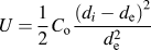$U = {1 \over 2}{C_{\rm{o}}}{{{{\left( {{d_i} - {d_{\rm{e}}}} \right)}^2}} \over {d_{\rm{e}}^2}}$.

The an-harmonic lattice forces that are needed to facilitate inelastic scatting transition are not included in the unperturbed Hamiltonian description but are accounted for in the perturbing potential, which is determined self-consistently. Often the higher order terms of the pair potential that comprise the an-harmonic terms are difficult to determine and often over-restrict the model or are simply used as fitting parameters.^{Reference Ziman17} The model developed in this research will include an-harmonicity through a scattering contact i.e., determined self-consistently.

The Hamiltonian is constructed by placing atoms at a position near the equilibrium lattice constant so that there is a divisible number of atoms within the layer. This inherently induces a strain in the system of atoms, inducing potential energy in the system. The Hamiltonian matrix is assembled in the same manner as the effective mass Hamiltonian, in that the matrix must remain Hermitian to obtain real eigenvalues. Knowing the potential energy at each lattice point and the mass of each atom, the following Hamiltonian matrix is assembled, 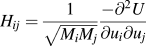${H_{ij}} = {1 \over {\sqrt {{M_i}{M_j}} }}{{ - {\partial ^2}U} \over {\partial {u_i}\partial {u_j}}}$. Here, M is the mass and U is the potential energy. The open channel equilibrium equation that is of interest is similar to the electron equilibrium equation except in the phonon model is framed in units of angular frequency; see the following equilibrium equation, (ω²I − H)u = 0. Here, ω² is the angular frequency squared of phonon eigenvalues, which relates to the discrete energy level of phonon energy. These eigenvalues describe the allowed modes within the channel region or the discrete phonon frequencies that are responsible for the transport.

The steps to calculate the phonon transport using NEGF are as follows, (i) the harmonic matrix is assembled, (ii) the eigenvalues are determined, (iii) the transmission probability for each phonon frequency that was defined by the eigenvalues is calculated, and (iv) the thermal transport energy and thermal conductivity are calculated. In reference to Eq. (1) and step 3, each phonon frequency has a finite thermal current governed by the phonon quantum conductance. The notion of a finite current at discrete energy levels is very similar to the case of a single electron level in the electron framework. The difference between the left and right transmission times the thermal quantum conductance is what governs the current carrying capacity of each discrete phonon frequency. The culmination of the transmission probabilities at discrete phonon frequencies gives rise to the overall calculated thermal conductivity of the device.

B. Phonon–phonon scattering

The phonon–phonon interaction is carried out by allowing each phonon frequency to scatter with each other. The superposition of all the scattering matrices in response to multiple phonon frequency scattering events culminates the overall scatter rate. The scattering rate for each phonon frequency is calculated using Fermi's golden rule. Fermi's golden rule states that the probability of scattering is dependent on the allowed transition from initial to final state and the available density of states of the final state. There are four transitions which are facilitated from the view point of a single spatial scattering site. They include the inflow (in-scattering) and the outflow (out-scattering) of scattered phonons. Both of these fluxes include two subtransitions, which are the absorption and emission of phonons. The selection rules in the model specify that the scattered phonon momentum must not be greater than the highest phonon frequency and must not be below the lowest scattering frequency. If this selection rule is not imposed, the scattered phonons will scatter to greater phonon frequencies above what is physically possible for the material. Additionally, an underlying assumption in the selection rules governs that the scattered phonons always scatter with a longitudinal phonon and scatter into a longitudinal state due to the fact the transport direct of interest is in the longitudinal direction.

Fermi's golden rule is written as a self-energy contact term, so the scattering sites can be incorporated as an additional contact along the device at every cell center in the overall Green's function. The perturbing potential or self-energy term seen in scattering contact, called a sigma term, includes a scattering factor (f _o) to govern the amplitude of the scattered phonon for a given phonon–phonon scattering event. The scattering parameter governs the strength of the an-harmonicity in the lattice and is a free parameter of the phonon scattering model. If the factor f _o increases, the scattering rate increases, resulting in decreased transport between the device contacts. The response of this parameter will be determined in the results section along with an optimal value for the given material. This term varies from zero (no scattering) and increases until the scattering saturates the transport and all phonons are scattered into the scattering contacts.

(2)$$\Sigma _{{\rm{s,ph}}}^{{\rm{in,out}}} = \int_{\hbar {\omega _{{\rm{min}}}}}^{\hbar {\omega _{{\rm{max}}}}} {{{{\rm{d}}\left( {\hbar \omega } \right)} \over {2\pi }}{f_{\rm{o}}}\left[ {\left( {{N_\omega } + 1} \right){G^{{\rm{n,p}}}}\left( {E + \hbar \omega } \right) + {N_\omega }{G^{{\rm{n,p}}}}\left( {E - \hbar \omega } \right)} \right]} \quad .$$

The model handles the calculation of self-energy scattering term, Σ_s by performing matrix manipulations on the filled (G ⁿ) and unfilled (G ^p) density of states to represent the final density of states. The final density of states can either be an absorption $\left( {E + \hbar \omega } \right)$, the shifting of matrices down the energy axis, or an emission $\left( {E - \hbar \omega } \right)$, the shifting of matrices values up in energy. These new matrices, [G ⁿ$\left( {E \;\pm\; \hbar \omega } \right)$ and G ^p$\left( {E \;\pm\; \hbar \omega } \right)$], define the final states. The shifting of matrices is carried out for all phonon frequencies to account for all the possible scattering interactions. Because phonons are bosonic, the term G ^p, which defines the unfilled states where A = G ^p + G ⁿ must be slightly modified from the electron formalism that is commonly found in the literature. In the previous equation, A is the local density of states, which is calculated from the difference between the retarding and advancing Green's function. The modification to the phonon formalism comes by making G ^p = A, describing the situation that the phonons can scatter into any state. This comes from the fact that phonons are bosonic quasi-particles.

The model incorporates the new scattering term (Σ_s,ph), a series of contacts along the device channel at the cell centers. This is often times referred to as the Butticker approximation and allows the inflow and outflow of energy at each cell center through the scattering contact. In addition to adding a contact, the model needs to make sure that the thermal energy is conserved in the system. The energy entering and leaving the contacts and scattering sites must add up to zero. An unknown Fermi function that defines the rate of inflow and outflow through the scattering contacts is used to conserve energy. The unknown Fermi function (f _s) for the contacts is determined iteratively and used to govern energy conservation. The solution is iterated self-consistently until the scattering solution has converged. Once a solution is found, the overall scattering rates and the thermal conductivity can be calculated.

C. Electron model

Similar to the phonon transport, a one-dimensional NEGF model is used to calculate the electronic transport. In the electronic model, an effective mass description is used and the electron–phonon interaction of multiple phonon frequencies is accounted. In the effective mass description, the only variable that influences the eigenvalues is the effective mass of the electron and the geometry. The effective mass will be assumed parabolic and because of the 1D description, only a single effective mass along the $\left\langle {001} \right\rangle$ crystallographic direction is used (see the Supplemental Material for specific model parameters). The model assumes that both spin states are filled so that the material is spin degenerate. The Hamiltonian will have a different effective mass for each material. At the interface of two materials there exists a node with an average of the two neighboring effective masses. The Hamiltonian description takes the following form, $H = {{{\hbar ^2}} \over {2{m^*}{a^2}}}$. Here, a defines the lattice spacing between grid points. This model is not an atomistic formalism but an energy discretization. The grid spacing is only dependent on the desired frequency content or energy range of interest.

To calculate the current between the temperature contacts, an integral expression similar to the expression used for the phonon current is used. That expression is,

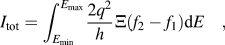(3)$${I_{{\rm{tot}}}} = \int_{{E_{{\rm{min}}}}}^{{E_{{\rm{max}}}}} {{{2{q^2}} \over h}\Xi \left( {{f_2} - {f_1}} \right){\rm{d}}E} \quad ,$$

where the transmission for a single electron is summed across a range of electron energies to arrive at the overall current. The applied voltage and temperature boundary conditions are defined by either Fermi Dirac terms f ₁ and f ₂.

By initially specifying a temperature gradient at either contact, the system begins at a nonequilibrium state. The Fermi functions defined at either contact are specified with a temperature difference, imposing nonequilibrium on the system. A resulting current is calculated using Eq. (3) for electron energy of −0.4 to 1 eV spanning the lowest conduction levels and 3k _bT above the highest conduction band of the system.

The calculation begins by determining the electrical current at zero voltage bias with a specified temperature bias defining the electrical contribution of the thermal conductivity, k _e. Next, a voltage in the opposite direction of the temperature bias is incrementally increased until the current across the system becomes zero, defining the Seebeck voltage of the structure. Additionally, the electrical conductivity is determined by calculating the slope of the IV curve near the Seebeck voltage using a forward difference.

D. Electron–phonon scattering

In the fully coupled system, a major aspect that is missing is the rate at which the electrons and phonons interact. Note, the following formalism describes the steady-state interactions of electrons and phonons. To incorporate the phase-breaking operation in which the background (phonons) interacts with the electrons, a slightly more complicated view point must be taken from the perspective of the electron model.

The scattering theory used in this model is based on a self-consistent Born approximation (SCBA) to determine the scattering matrices. It has been demonstrated by researchers^{Reference Datta19,Reference Lee and Venkatasubramanian20} that the SCBA theory has a wide range of validity and can apply to weakly and strongly coupled electrons and phonons. The limitations on the SCBA theory can only be determined by comparing to experimental results. From this understanding, it is assumed that SCBA is valid for the Si/Ge single crystal nanostructured thermoelectric materials of interest in this research and will be validated based on comparison to literature values.

The overall Hamiltonian of the coupled system that describes the electron–phonon interaction has the form, H = H _p + H _e + H _ei. Here, H _p describes the oscillators (phonons) and H _e describes electrons and H _ei describes the electron phonon interaction. Writing the Hamiltonian in second quantization,^{Reference Mahan15} the following terms can be partitioned so that the electron NEGF model solves H _e + H _ei and the phonon NEGF solves the remaining H _p. The electronic Green's functional model which includes the electron–phonon interaction can be written as follows, G = (EI − H − U _ee − Σ₁ − Σ₂ − Σ_s)⁻¹. Here, Σ₁ and Σ₂ are the in-scattering from the contacts and Σ_s is the in-scattering from the phonons, treating the in-scattering due to phonons as multiple contacts (Butticker probes) located along the length of the device. Because the equilibrium energy of the phonon contacts is unknown, a self-consistent method is need to determine a rate term for the phonon contacts. This is critical and can be conceptualized as a Fermi term for the phonon contacts. This Fermi contact term is determined through Kirchhoff's law in which all the energy entering and leaving the source and drain contact must balance with the energy leaving or energy from the scattering contacts. An assumption has been made that there is a single rate term for the whole phonon contact or all phonon frequencies.

E. Buttiker approximation

The calculated spectral function for both the electrons and phonons will give rise to the probability at which the electrons and phonons scatter through the Fermi's golden rule expression. Assuming that the phonons and electrons interact along discrete cell centers as if contacts were placed along the length of the device, one can make the analogy that there is a Butticker probe attached at each discretized cell center. These probes provide a means of in-scattering and out-scattering along the length of the device. Each of these scattering contacts have an associated delta potential that allows the interband and intraband transition to be facilitated with the creation or annihilation of phonons. The probability of these transitions is dependent on the phonon scattering energy and the shifting of the density of states. The intraband transition is not handled rigorously like the interband, however, energy is allowed to scatter out of the system and then allowed to scatter back in at a later band.

In other's research,^{Reference Datta13,Reference Bulusu and Walker21,Reference Koswatta, Hasan, Lundstrom, Anantram and Nikonov22} the Σ_s,e term is calculated using a single phonon frequency with a deformation potential approach and the Bose–Einstein dispersion relation to determine the number of phonons. The approach in this study is similar, except multiple phonon frequencies will be included. This is critical in layered structures where the electron–phonon tunneling influences the transport significantly.

(4)$$\Sigma _{{\rm{s,e}}}^{{\rm{in,out}}} = \int_{{E_{{\rm{min}}}}}^{{E_{{\rm{max}}}}} {{{{\rm{d}}\left( {\hbar \omega } \right)} \over {2\pi }}{D_{\rm{o}}}\left( {\hbar \omega } \right)\left[ {\left( {{N_\omega } + 1} \right){G^{{\rm{n,p}}}}\left( {E + \hbar \omega } \right) + {N_\omega }{G^{{\rm{n,p}}}}\left( {E - \hbar \omega } \right)} \right]} \quad .$$

Equation (4) is the sigma scattering term used. The factor D _o is comprised of the phonon density of states and a deformation constant, which is responsible for the strength of the scattering. This approach, often called deformation theory, is a proven method of accounting for electron–phonon scattering. The deformation potential provides a potential response due to the presence of a particular phonon frequency. Thus, if multiple phonon frequencies are incorporated, multiple potential responses are possible. This research will assume that the superposition of multiple responses is related to the scattering of a single scatting site along the device.

There are two types of deformation potentials, acoustic and optical, which are selected based on the type of interaction. The deformation potential was selected based on an optical cut-off frequency. If the incoming scattering phonon is below the optical cut-off frequency it was assumed acoustic and the acoustic deformation potential was used. Likewise, if the incoming phonon frequency was greater than the cut-off, the optical deformation was used. The deformation potential is thought of as the potential response due to the presence of phonon, which corresponds to a localized lattice strain. Because the lattice strain is different for optical phonons, where the neighboring atoms oscillate opposite each other, and acoustic phonons, where neighboring atoms oscillate in the same direction, there are two different deformation potentials. The acoustic deformation potential takes the following form, $D_{{\rm{adp}}} = {{D_{\rm{a}}^2 \beta ^2 q} \mathord{\left {\vphantom {{D_{\rm{a}}^2 \beta ^2 q} {24\rho \nu _{\rm{s}} }}} \right. \kern-\nulldelimiterspace}/ {24\rho \nu _{\rm{s}} }}$, where D _a is the tabulated acoustic deformation potentials factor determined from experimental studies.^{Reference Jacoboni and Reggiani23,Reference Jacoboni, Cananli, Ottaviani and Quaranta24} The term β is the wave-vector and ρ is the density of the material and ν_s is the sound speed of the material. The optical deformation potential is similar except the deformation factor D _odp has different units. The optical deformation takes the following form, $D_{{\rm{odp}}} = {{D_{\rm{o}}^2 \beta ^2 q} \mathord{\left {\vphantom {{D_{\rm{o}}^2 \beta ^2 q} {16\rho \omega _{\rm{o}} }}} \right. \kern-\nulldelimiterspace}/ {16\rho \omega _{\rm{o}} }}$, where ω_o is the cut-off frequency for optical phonons. Both of these deformation potentials were calculated based on the scattering rate for both optical and acoustic phonons from a density of states description.^{Reference Lundstrom25}

The approach by Bulusu and Walker^{Reference Bulusu and Walker21} and Koswatta et al.^{Reference Koswatta, Hasan, Lundstrom, Anantram and Nikonov22} focused on using a single deformation potential as a mean of fitting the experimental data because they only dealt with a single phonon frequency to encompass all phonon frequencies in the actual structure or just the dominate phonon frequency. They also limited their scattering to the optical phonon scattering, which may be a valid assumption, but more modes can be captured in the forthcoming method, resolving transitions absent in their calculation.

To increase the fidelity of Eq. (4), the approach taken in this work is to couple the NEGF phonon solution to the NEGF electron model and account for more than one phonon frequency. The NEGF phonon method calculates the dominate phonon modes of the structure and the associated spatially varying correlation matrices, allowing multiple phonon modes to be coupled. Because the correlation matrices provide the density of filled phonon states (G ⁿ) and empty phonon states (G ^p) a greater fidelity in the model can be resolved because the phonon distribution no longer relies on the equilibrium Bose–Einstein equation. The following expression is what would be required to couple the output from the phonon NEGF to the electron NEGF.

In the sigma term, the G ⁿ$\left( {E - \hbar \omega } \right)$ terms are determined by shifting the correction matrix by the corresponding phonon energy, $\hbar \omega$, to take the view point of that final state. The sigma terms can be combined into a single gamma term using the following expression, ${\Gamma _{{\rm{s,e}}}} = \Sigma _{{\rm{s,e}}}^{{\rm{in}}} + \Sigma _{{\rm{s,e}}}^{{\rm{out}}}$. Additionally, the sigma term can be related back to the Boltzmann description as the scattering term, $\Gamma _{{\rm{s,e}}} = S^{{\rm{in}}} \hbar = {\hbar \mathord{\left/ {\vphantom {\hbar \tau }} \right. \kern-\nulldelimiterspace} \tau }$.

F. Complex contacts

An important aspect of both the phonon and electron formalism is the definition of the scattering contacts. The overall scattering term is the summation of the in-scattered (Σⁱⁿ) and the out-scattered (Σ^out) terms determined from Fermi's golden rule. Additionally, the Σ terms are complex and take the form of, σ + iγ, where σ is a real term and γ is an imaginary term. The Σ terms are in the time domain and require that they are transformed to the frequency domain so that they can be applied to the Green's function as boundary conditions. To apply the transformation, an approximate Hilbert transformation is carried out involving a Fourier transform. The scattering boundary takes the form of a matrix, where the main diagonal is determined using, $G_{{\rm{s,e}}} = {{\Sigma _{{\rm{s,e}}}^{{\rm{in}}} } \mathord{\left/ {\vphantom {{\Sigma _{{\rm{s,e}}}^{{\rm{in}}} } {f_{\rm{s}} }}} \right. \kern-\nulldelimiterspace} {f_{\rm{s}} }} - {{0.5i\left( {\Sigma _{{\rm{s,e}}}^{{\rm{in}}} - \Sigma _{{\rm{s,e}}}^{{\rm{out}}} } \right)} \mathord{\left/ {\vphantom {{0.5i\left( {\Sigma _{{\rm{s,e}}}^{{\rm{in}}} - \Sigma _{{\rm{s,e}}}^{{\rm{out}}} } \right)} {f_{\rm{s}} }}} \right. \kern-\nulldelimiterspace} {f_{\rm{s}} }}$.

This is an approximation of the actual Hilbert transformation because the function of the integral is unknown and therefore the imaginary part is approximated as 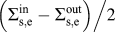${{\left( {\Sigma _{{\rm{s,e}}}^{{\rm{in}}} - \Sigma _{{\rm{s,e}}}^{{\rm{out}}} } \right)} \mathord{\left/ {\vphantom {{\left( {\Sigma _{{\rm{s,e}}}^{{\rm{in}}} - \Sigma _{{\rm{s,e}}}^{{\rm{out}}} } \right)} 2}} \right. \kern-\nulldelimiterspace} 2}$. This approximation is justified because the scattering contacts are determined self-consistently. This approximation was avoided in the source and drain contacts because the known analytic expression was used to describe the contact. Additional research is required to justify this approximation but is beyond the scope of this initial study.

G. Coupled model implementation

Three models of increasing degree of electron–phonon interactions were considered for this research. The first model was a ballistic treatment that included no electron–phonon interaction. The second model was a single user-specified optical phonon frequency scattering. The third model was a two-way model where multiple phonons were passed from the phonon model to the electron model to facilitate multiple scattering with the added complexity of passing back the scattered energy for each electronic subband.

In single phonon coupling, the user-specified phonon energy is 62 meV in silicon and 34 meV in germanium. The electron model only facilitated electron–phonon interaction of a single phonon frequency. The phonon model included phonon–phonon interaction with no influence from the electrons. The electron NEGF model is similar to the models used by Bulusu and Walker and Koswatta et al.^{Reference Bulusu and Walker21,Reference Koswatta, Hasan, Lundstrom, Anantram and Nikonov22}

The two-way coupling model requires the phonon model to pass the phonon correlation function $\left( {G_{{\rm{ph}}}^{{\rm{n,p}}}} \right)$ of the normal mode phonon frequencies after each electronic subband calculation. This correlation function included the local density description of all the phonon frequencies. In addition to passing the phonon information, the electron–phonon energy scattered out of the electronic model was exchanged to the phonon model as input phonon energy. This requires that the electron and phonon model be run simultaneously, communicating at each subband calculation. The two models continued until convergence of the electronic current were reached.

All the message passing between the two models was handled using a producer–consumer message passing model. The passing involved a status file from both the phonon model and electron model that altered the status of available data or ready to receive data. If spatial grid data were being passed between codes, an additional step in formatting the data was required. This additional step was a result of the different grid discretization of the phonon (atomistic) and the electron models. In addition to the spatial interpolation, the energy discretization of the two models also had to be interpolated. All the interpolation was done by using a Hermite polynomial interpolation for each phonon frequency in the spatially direction, followed by an interpolation in the energy axis resulting in an overall surface interpolation.

H. Superlattice results

The Seebeck coefficient and electrical conductivity were calculated for varying donor concentrations (n-type, phosphorous doped) for several superlattice configurations found in the literature. Results are shown in Fig. 2 for three models which include ballistic, single phonon, and multiple phonon scattering models. All of these experimental and computational values are at an average temperature of 300 K. Also, provided within the figure is the Si_0.8 Ge_0.2 alloy value at 300 K for reference. In the case of the Seebeck coefficient as seen in Fig. 2, as the degree of electron–phonon scattering is increased to include multiple phonon frequencies, the Seebeck coefficient subsequently increases. This increase is attributed to a change in electron gradient across the structure. By investigating the localize scattering rate near the leading edge of the barrier material, there is a noted increase in the electron–phonon scattering. This increased interaction leads to the increased gradient of electrons and in turn greater Seebeck coefficient. The experimental data points provided in the Figures render a relative comparison and validation of the computational predictions. However, the reader should note the scatter in the experimental data, which is associated with the uncertainty in the experimental fabrications and measurements of nanoscale samples. While the experimental uncertainty was not quantified in these studies, confidence in the computational results is gathered by the intersection of the experimental and computational data. What the computational data does provide is the prediction for the whole range of donor concentrations, which is not available from the experimental data.

FIG. 2.

Plot of Seebeck coefficient as a function of donor concentration for several superlattice configurations at 300 K. The lines correspond to the three models, ballistic, single, and multiple phonon frequency scattering. The multiple frequency scattering increased the Seebeck coefficient due to the increased spatial variation of charges.

Aside from the Seebeck coefficient, the electrical conductivity (see Fig. 3) and the electronic and thermal contribution to the thermal conductivity (see Fig. 4). One of the real advantages of these nanostructured superlattices is to diminish the lattice contribution to the thermal conductivity as result of the increased boundary scattering. As seen in Fig. 3, the electrical conductivity nearly six orders of magnitude over the concentration range. Similarly, the electron contribution (k _e) to the thermal conductivity as depicted in Fig. 4 undergoes a proportional change. This proportional change is often the crux of developing good performing thermal electric materials. It is interesting to note from Fig. 4 that phonon model predicts the diminished lattice contribution as a result of the superlattice interfaces and confined phonon states, however, in the case of the ballistic model the total thermal conductivity (k _e + k _p) is dominated by the electronic contribution. In the case of the multiphonon model, the electrical conductivity is decreasing along with the k _e and therefore the lattice contribution (k _p) has a noticeable contribution at low donor concentrations. This noticeable contribution of the overall thermal conductivity is directly corresponds to a maximum in the ZT, see Fig. 5.

FIG. 3.

Plot of electrical conductivity as a function of donor concentration for several superlattice configurations at 300 K. The multiple frequency scattering case decreases the electrical conductivity to a level that was comparable to the thermal conductivity.

FIG. 4.

Thermal conductivity for the corresponding superlattice materials. The open symbols are the calculated electronic contribution to the thermal conductivity (k _e) and the solid symbols are the combined electronic plus lattice contribution (k _e + k _p) to the overall thermal conductivity. The lattice contribution (k _p) is provided in the figure, however, there is no dependence with doping concentration.

FIG. 5.

ZT calculation of several superlattice materials. Temperature was held at 300 K. For the multiple frequency scattering case there is an extrema in the ZT, which is similar to what is found experimentally. This extrema is an indication that the geometry for given doping concentration can be optimized.

Figure 3 is a similar plot to the Seebeck plot, however, electrical conductivity is plotted against donor concentration. Here, the multiple phonon frequency model induces a decrease in the electrical conductivity. The conductivity values are in turn more comparable to literature values as the ballistic case severely overestimates the conductivity. Focusing on Fig. 5 of the ZT as a function of doping, the multiple phonon frequency scattering case has the largest ZT response. In fact, the multiple phonon case resolves an extreme in the ZT. The extrema is a function of both the geometry and the doping. For a case, when a 5 nm/7 nm Si/Ge superlattice is constructed the doping concentration in layers should be on the order of 10²⁰ cm⁻³. For 8 nm/2 nm, the maximum is at a doping concentration of 10²⁰ cm⁻³. However, for 2 nm/2 nm, the maximum is near 10¹⁸ cm⁻³. This increase in ZT at lower doping concentration is most likely attributed to the increased conductivity of the 2 nm/2 nm. It is interesting to note that as the Si thickness increases from 2 nm/2 nm to the 8 nm/2 nm case, the extrema shifts. Furthermore, both the Seebeck and electrical conductivity decrease compared to 2 nm/2 nm case. Therefore, to recover the electronic conductivity diminished by the increase in silicon well length, the donor concentration must be increased. However, this is up to a certain level until both the Seebeck and the electronic contribution to the thermal conductivity decrease the ZT.

It is interesting to note that the true optimal silicon germanium superlattice spacing has never been explained or exhausted from an experimental perspective. It is reasoned from these computational results that the best superlattice thermoelectric design would have a ZT response that peaks in the middle, straddling the whole donor concentration region. It is hypothesized that the corresponding structure to achieve this would be a 2 nm/7 nm, a structure with a small silicon layer and a larger germanium. The 7 nm germanium layer would be aimed at shifting the 2 nm/2 nm peak toward 10¹⁹ cm⁻³. This shift is evident with increasing barrier thickness by comparing the 8 nm/2 nm case with the 5 nm/7 nm case, granted the second case has a slightly larger 5 nm silicon thickness.