2.1. Governing equations

In this subsection, we introduce the physical models and governing equations used in this study. Theoretically, the Bhatnagar–Gross–Krook (BGK)–Maxwell system can be used to model the partially ionised plasma (Pu & Xu Reference Pu and Xu2025),

(2.1) \begin{equation} \begin{aligned} & \frac {\partial f_\alpha }{\partial t}+\boldsymbol{u}_\alpha \boldsymbol{\cdot }\boldsymbol{\nabla} _{\!\boldsymbol{x}} f_\alpha + \frac {q_\alpha (\boldsymbol{E}+\boldsymbol{u}_\alpha \times \boldsymbol{B})}{m_\alpha } \boldsymbol{\cdot }\boldsymbol{\nabla} _{\!\boldsymbol{u}} f_\alpha = Q_{\alpha }, \\ & \frac {\partial \boldsymbol{B}}{\partial t}+\boldsymbol{\nabla} _{\!\boldsymbol{x}} \times \boldsymbol{E}=0, \quad \frac {\partial \boldsymbol{E}}{\partial t}-c^2 \boldsymbol{\nabla} _{\!\boldsymbol{x}} \times \boldsymbol{B}=-\frac {1}{\epsilon _0} \boldsymbol{J}, \\ &\boldsymbol{\nabla} _{\!\boldsymbol{x}} \boldsymbol{\cdot }\boldsymbol{E}=\frac {\rho _c}{\epsilon _0},\quad \boldsymbol{\nabla} _{\!\boldsymbol{x}} \boldsymbol{\cdot }\boldsymbol{B}=0, \end{aligned} \end{equation}

where $f_\alpha = f_\alpha (t, \boldsymbol{x}, \boldsymbol{u})$ is the microscopic distribution function for species $\alpha$ ( $\alpha =i$ for ion and $\alpha =e$ for electron, $\alpha =n$ for atom) at space and time $(\boldsymbol{x},t)$ , and microscopic translational velocity $\boldsymbol{u}$ ; $q_\alpha$ is the charge carried by species $\alpha$ ; $\boldsymbol{E}, \boldsymbol{B}$ is the electric and magnetic field strength; $\epsilon _0$ is the permittivity of free space and $c$ is the light speed; $\boldsymbol{J}$ is the electric current density; $\rho _c$ is the electric charge density. Here, $Q_{\alpha }=\sum _{k\neq \alpha }Q_{\alpha k}(f_\alpha, f_k)$ is the collision operator of species $\alpha$ between species $k$ , approximated by the Andries–Aoki–Perthame (AAP) model (Andries, Aoki & Perthame Reference Andries, Aoki and Perthame2002),

(2.2) \begin{equation} Q_\alpha =\frac {g_\alpha ^M-f_\alpha }{\tau _\alpha }, \end{equation}

where $g_\alpha ^{M}$ is a Maxwellian distribution,

(2.3) \begin{equation} g_\alpha ^M=\rho _\alpha\! \left (\frac {m_\alpha }{2 \pi\! k \bar {T}_\alpha }\right )^{3 / 2} \exp\! \left (-\frac {m_\alpha }{2 k_B \bar {T}_\alpha }\left (\boldsymbol{u}_\alpha -\bar {\boldsymbol{U}}_\alpha \right )^2\right )\!, \end{equation}

and post-collision velocity $\bar {\boldsymbol{U}}_\alpha$ and temperature $\bar {T}_\alpha$ are given as

(2.4) \begin{align} \begin{aligned} \bar {\boldsymbol{U}}_\alpha & =\boldsymbol{U}_\alpha +\frac {\tau _\alpha }{m_\alpha } \sum _{k=1}^N 2 \mu _{\alpha k} \chi _{\alpha k} n_k \! \left (\boldsymbol{U}_k-\boldsymbol{U}_\alpha \right )\!, \\ \bar {T}_\alpha & =T_\alpha -\frac {m_\alpha }{3 k_B}\left (\bar {\boldsymbol{U}}_\alpha -\boldsymbol{U}_\alpha \right )^2+\tau _\alpha \sum _{k=1}^N \frac {4 \mu _{\alpha k} \chi _{\alpha k} n_k}{m_\alpha +m_k}\left (T_k-T_\alpha +\frac {m_k}{3 k_B}\left (\boldsymbol{U}_k-\boldsymbol{U}_\alpha \right )^2\right )\!, \end{aligned} \end{align}

where $\mu _{\alpha k} = m_{\alpha }m_k/(m_{\alpha }+m_k)$ is reduced mass, $N$ is number of species in the system. Species $\alpha$ ’s mean relaxation time $\tau _\alpha$ is determined by $1 / \tau _\alpha =\sum _{k=1}^m \chi _{\alpha k} n_{k}$ , and interaction coefficient $\chi _{\alpha k}$ for the variable hard sphere (VHS) model is (Morse Reference Morse1963)

(2.5) \begin{equation} \chi _{\alpha k}= \frac {(5-2\omega )(7-2\omega )\sqrt { \pi }}{15}\left (\frac {2 k_B T_{\alpha }}{m_\alpha }+\frac {2 k_B T_{k}}{m_k}\right )^{1 / 2}\left (\frac {d_\alpha +d_k}{2}\right )^2 \!, \end{equation}

where $ d_\alpha, d_k$ are the diameters of the particles. The temperature modifies the molecular diameter as $ ({d}/{d_{\textit{ref}}})^2 = ( {T}/{T_{\textit{ref}}} )^{({1}/{2}) - \omega },$ where $\omega$ is the power coefficient between viscosity and temperature (Bird Reference Bird1976). Specific diameters for each species are presented in the subsequent numerical studies. For complex interactions involving neutral and charged species, experimentally derived fitted curves will be employed and presented in the numerical study section. The AAP model exhibits a Prandtl number of unity. Future work will extend the multi-relaxation-time, multi-species kinetic model to more accurately capture the simultaneous behaviour of viscosity and thermal conductivity, referencing work such as Bisi et al. (Reference Bisi, Boscheri, Dimarco, Groppi and Martalò2022) and Li, Zeng & Wu (Reference Li, Zeng and Wu2024).

For hypersonic applications, the BGK–Maxwell system can be simplified. In many such applications, the ionised gas within the shock layer exhibits low electrical conductivity $\sigma ^{\textit{cond}}$ (Poggie & Gaitonde Reference Poggie and Gaitonde2002). This leads to a small induced current density $\boldsymbol{J}$ according to the Ohm’s law $\boldsymbol{J} = \sigma ^{\textit{cond}}(\boldsymbol{E}+\boldsymbol{U}\times \boldsymbol{B})$ . Consequently, the magnetic field produced by this current is significantly weaker than the externally applied magnetic field $\boldsymbol{B}_{\textit{ext}}$ . This allows for the neglect of magnetic field distortion by the flow field, enabling the assumption of a static magnetic field for the present investigation. Faraday’s law can be neglected since the static magnetic field will generate no transverse electric field. Furthermore, the hyperbolic divergence cleaning technique realises the charge neutrality (Munz et al. Reference Munz, Omnes, Schneider, Sonnendrücker and Voss2000):

(2.6) \begin{align} \epsilon _0\frac {\partial \boldsymbol{E}}{\partial t} + c^2\boldsymbol{\nabla }\phi = -\boldsymbol{J},\quad \frac {\partial \phi }{\partial t} + \boldsymbol{\nabla }\boldsymbol{\cdot }\boldsymbol{E} = \frac {\rho _c}{\epsilon _0}, \end{align}

where $\phi$ is the artificial correction potential. An approximate Debye length of $10^{-4}$ m is implemented to alleviate numerical stiffness. Therefore, the final form of the physical model is given as

(2.7) \begin{equation} \begin{aligned} & \frac {\partial f_\alpha }{\partial t}+\boldsymbol{u}_\alpha \boldsymbol{\cdot }\boldsymbol{\nabla} _{\!\boldsymbol{x}} f_\alpha + \frac {q_\alpha (\boldsymbol{E}+\boldsymbol{u}_\alpha \times \boldsymbol{B}_{\textit{ext}})}{m_\alpha } \boldsymbol{\cdot }\boldsymbol{\nabla} _{\!\boldsymbol{u}} f_\alpha = Q_{\alpha }, \\ &\epsilon _0\frac {\partial \boldsymbol{E}}{\partial t} + c^2\boldsymbol{\nabla }\phi = -\boldsymbol{J},\quad \frac {\partial \phi }{\partial t} + \boldsymbol{\nabla }\boldsymbol{\cdot }\boldsymbol{E} = \frac {\rho _c}{\epsilon _0}. \end{aligned} \end{equation}

In the fluid limit $\tau _{\alpha } \rightarrow 0$ , (2.7) turns to a multi-fluid equation as

(2.8) \begin{equation} \begin{aligned} & \partial _t \rho _n+\boldsymbol{\nabla} _{\!\boldsymbol{x}} \boldsymbol{\cdot }\left (\rho _n \boldsymbol{U}_n\right )=0, \\ & \partial _t\left (\rho _n \boldsymbol{U}_n\right )+\boldsymbol{\nabla} _{\!\boldsymbol{x}} \boldsymbol{\cdot }\left (\rho _n \boldsymbol{U}_n \boldsymbol{U}_n+p_n \mathbb{I}\right )=R_n, \\ & \partial _t \mathscr{E}_n+\boldsymbol{\nabla} _{\!\boldsymbol{x}} \boldsymbol{\cdot }\left (\left (\mathscr{E}_n+p_n\right ) \boldsymbol{U}_n\right )=S_n,\\ & \partial _t \rho _i+\boldsymbol{\nabla} _{\!\boldsymbol{x}} \boldsymbol{\cdot }\left (\rho _i \boldsymbol{U}_{\!i}\right )=0, \\ & \partial _t\left (\rho _i \boldsymbol{U}_{\!i}\right )+\boldsymbol{\nabla} _{\!\boldsymbol{x}} \boldsymbol{\cdot }\left (\rho _i \boldsymbol{U}_{\!i} \boldsymbol{U}_{\!i}+p_i \mathbb{I}\right )=q_in_i\left (\boldsymbol{E}+\boldsymbol{U}_{\!i} \times \boldsymbol{B}_{\textit{ext}}\right )+R_i, \\ & \partial _t \mathscr{E}_i+\boldsymbol{\nabla} _{\!\boldsymbol{x}} \boldsymbol{\cdot }\left (\left (\mathscr{E}_i+p_i\right ) \boldsymbol{U}_{\!i}\right )=q_in_i \boldsymbol{U}_{\!i} \boldsymbol{\cdot }\boldsymbol{E}+S_i,\\ & \partial _t \rho _e+\boldsymbol{\nabla} _{\!\boldsymbol{x}} \boldsymbol{\cdot }\left (\rho _e \boldsymbol{U}_e\right )=0, \\ & \partial _t\left (\rho _e \boldsymbol{U}_e\right )+\boldsymbol{\nabla} _{\!\boldsymbol{x}} \boldsymbol{\cdot }\left (\rho _e \boldsymbol{U}_e \boldsymbol{U}_e+p_e \mathbb{I}\right )=q_en_e\left (\boldsymbol{E}+\boldsymbol{U}_e \times \boldsymbol{B}_{\textit{ext}}\right )+R_e, \\ & \partial _t \mathscr{E}_e+\boldsymbol{\nabla} _{\!\boldsymbol{x}} \boldsymbol{\cdot }\left (\left (\mathscr{E}_e+p_e\right ) \boldsymbol{U}_e\right )=q_en_e \boldsymbol{U}_e \boldsymbol{\cdot }\boldsymbol{E}+S_e, \\ &\epsilon _0\frac {\partial \boldsymbol{E}}{\partial t} + c^2\boldsymbol{\nabla }\phi = -\boldsymbol{J},\quad \frac {\partial \phi }{\partial t} + \boldsymbol{\nabla }\boldsymbol{\cdot }\boldsymbol{E} = \frac {\rho _c}{\epsilon _0}, \end{aligned} \end{equation}

where $\rho _\alpha, \boldsymbol{U}_\alpha, \mathscr{E}_\alpha$ represent the mass density, macroscopic velocity and energy density of species $\alpha$ , and $p_\alpha$ is the thermal pressure of species $\alpha$ . Here, $R_\alpha, S_\alpha$ are the source terms due to cross-species momentum and energy transfer. In the limit of a strong magnetic field, negligible electron mass and the non-relativistic regime, (2.7) simplifies to MHD equations. A detailed asymptotic analysis of this reduction is provided by Pu & Xu (Reference Pu and Xu2025).

2.2. UGKWP method

In this subsection, the UGKWP method to solve the system (2.7) as it transitions from the rarefied regime to the continuum regime is introduced. First, the multispecies collision operator is rewritten as

(2.9) \begin{equation} Q_\alpha = \frac {g_\alpha ^{eq}-f_\alpha }{\tau _\alpha } + \frac {g_\alpha ^M-g_\alpha ^{eq}}{\tau _\alpha }, \end{equation}

where $g^{eq}_\alpha$ is the Maxwellian distribution by collision within the same species and $g^M_\alpha$ is the Maxwellian distribution after collisions between different species. Then, the operator splitting method is used to solve system (2.7) and (2.9) with time step $\Delta t$ ,

(2.10) \begin{align} &\mathcal{L}_1: \frac {\partial f_\alpha }{\partial t}+\boldsymbol{u}_\alpha \boldsymbol{\cdot }\boldsymbol{\nabla} _{\!\boldsymbol{x}} f_\alpha = \frac {g_\alpha ^{eq}-f_\alpha }{\tau _\alpha }, \\[-12pt]\nonumber \end{align}

(2.11) \begin{align} &\mathcal{L}_2: \frac {\partial f_\alpha }{\partial t}+ \frac {q_\alpha (\boldsymbol{E}+\boldsymbol{u}_\alpha \times \boldsymbol{B}_{\textit{ext}})}{m_\alpha } \boldsymbol{\cdot }\boldsymbol{\nabla} _{\!\boldsymbol{u}} f_\alpha = 0,\quad \epsilon _0\frac {\partial \boldsymbol{E}}{\partial t} = -\boldsymbol{J}, \\[-12pt]\nonumber \end{align}

(2.12) \begin{align} &\mathcal{L}_3: \frac {\partial f_\alpha }{\partial t} = \frac {g_\alpha ^M-g_\alpha ^{eq}}{\tau _\alpha }, \\[-12pt]\nonumber \end{align}

(2.13) \begin{align} &\mathcal{L}_4:\epsilon _0\frac {\partial \boldsymbol{E}}{\partial t} + c^2\boldsymbol{\nabla }\phi = 0,\quad \frac {\partial \phi }{\partial t} + \boldsymbol{\nabla }\boldsymbol{\cdot }\boldsymbol{E} = \frac {\rho _c}{\epsilon _0}. \end{align}

The variables after each update are denoted as

(2.14) \begin{align} &\mathcal{L}_1: f^{n}_\alpha \rightarrow f^{*}_\alpha, \boldsymbol{W}^{n}_\alpha \rightarrow \boldsymbol{W}^{*}_\alpha, \quad \quad \;\; \mathcal{L}_2: f^{*}_\alpha \rightarrow f^{**}_\alpha, \boldsymbol{W}^{*}_\alpha \rightarrow \boldsymbol{W}^{**}_\alpha, \boldsymbol{E}^{n} \rightarrow \boldsymbol{E}^{*}, \nonumber \\ &\mathcal{L}_3: f^{**}_\alpha \rightarrow f^{n+1}_\alpha, \boldsymbol{W}^{**}_\alpha \rightarrow \boldsymbol{W}^{n+1}_\alpha,\; \mathcal{L}_4: \boldsymbol{E}^{*} \rightarrow \boldsymbol{E}^{n+1},\phi ^{n} \rightarrow \phi ^{n+1}, \end{align}

where $\boldsymbol{W}_{\alpha } = (\rho _{\alpha }, \rho _{\alpha } \boldsymbol{U}_{\alpha }, \rho _{\alpha } \mathscr{E}_{\alpha })$ is mass, momentum and energy densities of species $\alpha$ .

First, we introduce algorithms for solving $\mathcal{L}_1$ . For simplicity, the species subscript $\alpha$ is omitted here. The BGK equation without the force term is written as

(2.15) \begin{align} \frac {\partial f}{\partial t}+\boldsymbol{u} \boldsymbol{\cdot }\boldsymbol{\nabla} _x f = \frac {g-f}{\tau }, \end{align}

the time-dependent solution of the distribution function at the interface can be written as

(2.16) \begin{equation} f\left (\boldsymbol{x},\boldsymbol{u}, \boldsymbol{\xi }, t\right )=\frac {1}{\tau } \int _{0}^{t} g(\boldsymbol{x}^{\prime }, \boldsymbol{u}, \boldsymbol{\xi },t^{\prime }) e^{-\left (t-t^{\prime }\right ) / \tau }\, \mathrm{d} t^{\prime } + e^{-t / \tau } f_{0}\left (\boldsymbol{x}-\boldsymbol{u} t \right ), \end{equation}

where $\tau$ is the local mean relaxation time, $f_0$ is the initial gas distribution function at $t=0$ and $g$ is equilibrium distribution along the characteristic line $\boldsymbol{x}^{\prime } = \boldsymbol{x} - \boldsymbol{u} t^{\prime }$ . Expanding the equilibrium distribution function by the Taylor series to the second-order accuracy,

(2.17) \begin{equation} g^{\prime }=g+ {\boldsymbol{g}}_x \boldsymbol{\cdot }(\boldsymbol{x}^{\prime }-\boldsymbol{x})+g_t(t^{\prime }-t), \end{equation}

where $g\equiv g(\boldsymbol{x}, \boldsymbol{u},\boldsymbol{\xi }, t),g^{\prime }\equiv g(\boldsymbol{x}^{\prime }, \boldsymbol{u}, \boldsymbol{\xi }, t^{\prime })$ . By substituting them into (2.16), the numerical multiscale evolution solution for simulation particles can be obtained,

(2.18) \begin{equation} f(\boldsymbol{x}, \boldsymbol{u}, \boldsymbol{\xi }, t)=\left (1-e^{-t / \tau }\right ) g^{+}(\boldsymbol{x}, \boldsymbol{u}, \boldsymbol{\xi }, t )+e^{-t / \tau } f_{0}\left (\boldsymbol{x} - \boldsymbol{u}t\right ), \end{equation}

where

(2.19) \begin{align} g^{+} = g + \left ( \frac {\textit{te}^{- t\text{/}\tau }}{1 - e^{- t\text{/}\tau }} - \tau \right )\boldsymbol{u}\boldsymbol{\cdot }{\boldsymbol{g}}_x +\left ( \frac {t}{1 - e^{- t\text{/}\tau }} - \tau \right )g_t . \end{align}

Equation (2.19) describes the solution to the BGK equation, where the distribution function $f$ at time $t$ is a combination of the initial distribution function $f_0$ and the Taylor expansion of the equilibrium state $g$ . From the particles’ perspective, this equation implies that a particle has a probability of $e^{-t/\tau }$ to freely stream during the time interval $[0,t]$ , and a probability of $(1 - e^{-t/\tau })$ to collide with other particles. After multiple collisions, the particle distribution will reach the equilibrium state $g^+$ , whose degree of freedom can be degenerated.

Based on this physical picture, the UGKWP method represents the velocity distribution function in a micro–macro coupled way. A portion of the distribution is captured analytically through the equilibrium distribution function $g^+$ , while the remaining part is represented by stochastic simulation particles $P_k = (m_k, \boldsymbol{x}_k, \boldsymbol{u}_k)$ . Here, $m_k$ denotes the mass of simulation particle $P_k$ , which corresponds to a cluster of real gas particles of the same species, and $\boldsymbol{x}_k$ and $\boldsymbol{u}_k$ represent the position and velocity of the simulation particle $P_k$ , respectively.

According to (2.18), the cumulative distribution function of the particle’s free streaming time $t_{\!f}$ before the collision is given as

(2.20) \begin{align} F ( t_{\!f} \lt t) = \exp \left ( - t\text{/}\tau \right )\!, \end{align}

from which the free stream time $t_{\!f}$ can be sampled as $t_{\!f} = - \tau \ln (\eta )$ with $\eta$ a random varible subject to the uniform distribution $\eta \sim U(0,1)$ . For a time step $\Delta t$ , the particles with $t_{\!f} \geqslant \Delta t$ will undergo collisionless free streaming and the particles with $t_{\!f} \lt \Delta t$ will experience collisional interactions. The procedure of updating particles in the UGKWP method is as follows.

1. Step 1. During the time step, stream each particle $P_k$ for a time period of $\min (\Delta t, t_{\!f,k})$ . Then, identify and retain the collisionless particles, while removing the collisional particles. Calculate the free-transport flux across cell interfaces contributed by the particles and accumulate the total conservative quantities of the particles $\boldsymbol{W}_{\!i}^p$ .

2. Step 2. After updating the macroscopic conservative variables, calculate the total conservative quantities of the collisional particles $\boldsymbol{W}_{\!i}^h$ from the updated conservative quantities $\boldsymbol{W}_{\!i}$ as $\boldsymbol{W}_{\!i}^h = \boldsymbol{W}_{\!i} - \boldsymbol{W}_{\!i}^p$ .

3. Step 3. At the end of the time step, rebuild the velocity distribution. Calculate the analytical distribution $g^{+,c}$ and resample the collisionless particles from the distribution $g^{+,f}$ according to the updated conservative quantities, and sample the free-streaming time $t_{\!f,k}$ for each particle $P_k$ from the cumulative distribution function $F(t_{\!f} \lt t) = \exp (-t/\tau )$ $\boldsymbol{W}_{\!i}^h$ .

Refer to Pu & Xu (Reference Pu and Xu2025) for a more detailed description of the procedure. In the procedure already outlined, the algorithm for updating the macroscopic conservative variables is introduced in the following paragraph. The evolution of the microscopic velocity distribution is now solved numerically using particles.

Based on the finite volume framework, the cell-averaged macroscopic conservative variables on a physical cell $\varOmega _i$ are updated by the numerical flux through cell interfaces:

(2.21) \begin{equation} (\boldsymbol{W}_{\alpha })_i^{n+1} = (\boldsymbol{W}_{\alpha })_i^n - \frac {\Delta t}{|\varOmega _i|}\sum _{s\in \partial \varOmega _i}|l_s|(\mathscr{F}_{\boldsymbol{W}_\alpha })_s, \end{equation}

where $l_s\in \partial \varOmega _i$ is the cell interface with centre $\boldsymbol{x}_s$ and outer unit normal vector $\boldsymbol{n}_{s}$ ; $|l_s|$ is the area of the cell interface. The numerical flux across interface $(\mathscr{F}_{\boldsymbol{W}_\alpha })_s$ can be evaluated from distribution function at the interface,

(2.22) \begin{equation} (\mathscr{F}_{\boldsymbol{W}_\alpha })_s = \frac {1}{\Delta t}\int _{t^n}^{t^{n+1}}\boldsymbol{u}\boldsymbol{\cdot }\boldsymbol{n}_sf_\alpha (\boldsymbol{x}_{s},\boldsymbol{u},\boldsymbol{\xi },t)\boldsymbol{\varPsi } \mathrm{d}\boldsymbol{\varXi }\mathrm{d}t, \end{equation}

where $\boldsymbol{\varPsi }=(1,\boldsymbol{u}, ({1}/{2})(\boldsymbol{u}^2+\boldsymbol{\xi }^2))$ is the conservative moments of distribution functions and $\mathrm{d}\boldsymbol{\varXi }=\mathrm{d}\boldsymbol{u}\,d\boldsymbol{\xi }$ is the volume element in the phase space. For the cell interface $l_s$ , the distribution function $f_\alpha (\boldsymbol{x}_{s},\boldsymbol{u},\boldsymbol{\xi },t)$ cannot be analytically represented in the transitional and collisionless regimes, thus requiring direct tracking of its evolution as introduced in the previous paragraph. This numerical flux of the macroscopic conservative variable can be split into the equilibrium flux and free streaming flux according to (2.16). The equilibrium flux is

(2.23) \begin{equation} (\mathscr{F}_{\boldsymbol{W}})_s^g = \frac {1}{\Delta t}\int _{t^n}^{t^{n+1}}\boldsymbol{u}\boldsymbol{\cdot }\boldsymbol{n}_s \left [\frac {1}{\tau } \int _{0}^{t} g(\boldsymbol{x}^{\prime }, \boldsymbol{u}, \boldsymbol{\xi },t^{\prime }) e^{-\left (t-t^{\prime }\right ) / \tau } \mathrm{d} t^{\prime }\right ] \boldsymbol{\varPsi } \,\mathrm{d}\boldsymbol{\varXi }\,\mathrm{d}t \end{equation}

and the free streaming flux is

(2.24) \begin{equation} (\mathscr{F}_{\boldsymbol{W}})_s^f = \frac {1}{\Delta t}\int _{t^n}^{t^{n+1}}\boldsymbol{u}\boldsymbol{\cdot }\boldsymbol{n}_s \left [e^{-t / \tau } f_{0}\left (\boldsymbol{x}-\boldsymbol{u} t \right )\right ] \boldsymbol{\varPsi } \,\mathrm{d}\boldsymbol{\varXi }\,\mathrm{d}t. \end{equation}

The equilibrium flux can be calculated directly from the macroscopic conservative variables. Assume in (2.22), $\boldsymbol{x}_{s} = \boldsymbol{0}$ and $t^{n} = 0$ , the equilibrium $g$ at the cell interface is obtained by conservation constraint

(2.25) \begin{align} \int _{}^{}{g\boldsymbol{\varPsi }}\,{\rm d}\boldsymbol{\varXi } = \int _{\boldsymbol{u} \boldsymbol{\cdot }\boldsymbol{n} \gt 0}^{}{g^{l}\boldsymbol{\varPsi }}\,{\rm d}\boldsymbol{\varXi } + \int _{\boldsymbol{u} \boldsymbol{\cdot }\boldsymbol{n} \lt 0}^{}{g^{r}\boldsymbol{\varPsi }}\,{\rm d}\boldsymbol{\varXi }. \end{align}

The spatial and time derivatives can be obtained,

(2.26) \begin{align} \int _{}^{}{g_x\boldsymbol{\varPsi }}\,{\rm d}\boldsymbol{\varXi } = \boldsymbol{W}_x, \quad \int _{}^{}{g_t\boldsymbol{\varPsi }}\,{\rm d}\boldsymbol{\varXi } = -\!\! \int _{}^{}\boldsymbol{u} \boldsymbol{\cdot }g_x\boldsymbol{\varPsi }\,{\rm d}\boldsymbol{\varXi }, \end{align}

where $g^{l}$ and $g^{r}$ are the equilibrium distributions according to the reconstructed left and right side conservative variables at cell interface $\boldsymbol{W}^{l},{\ \boldsymbol{W}}^{r}$ , and $\boldsymbol{W}_x$ is the reconstructed spatial derivative of conservative variables at cell interface. The van Leer limiter is used to achieve a second-order accuracy in space reconstruction. In regions with strong gradients, the limiter restricts the gradient to prevent unphysical oscillations. Substituting the reconstructed equilibrium distribution into the equilibrium flux, we have

(2.27) \begin{align} (\mathscr{F}_{\boldsymbol{W}})_s^g = \int _{}^{}\boldsymbol{u} \boldsymbol{\cdot }\boldsymbol{n}_{s}\left ( C_{1}g_{0} + C_{2}\boldsymbol{u} \boldsymbol{\cdot }{\boldsymbol{g}}_{0x} + C_{3}g_{0t} \right )\varPsi \,{\rm d}\boldsymbol{\varXi }, \end{align}

where the time integration coefficients are

(2.28) \begin{align} &C_{1} = \Delta t - \tau \big( 1 - e^{- \Delta t\text{/}\tau }\big), \\[-12pt]\nonumber \end{align}

(2.29) \begin{align} &C_{2} = 2\tau ^2 \big(1 - e^{- \Delta t\text{/}\tau }\big) - \tau \Delta t -\tau \Delta t e^{- \Delta t\text{/}\tau }, \\[-12pt]\nonumber \end{align}

(2.30) \begin{align} &C_{3} = \frac {\Delta t^2}{2} - \tau \Delta t + \tau ^2 \big(1-e^{\Delta t/\tau }\big). \end{align}

Next, we consider the free stream flux $(\mathscr{F}_{\boldsymbol{W}})_s^f$ . As stated in the last subsection, the initial distribution is represented partially by an analytical distribution $g_{a}^{+,c}$ and partially by particles, and therefore, the free stream flux is also calculated partially from the reconstructed analytical distribution as $(\mathscr{F}_{\boldsymbol{W}})_s^{f,w}$ and partially from particles as $(\mathscr{F}_{\boldsymbol{W}})_s^{f,p}$ . The initial analytical distribution $g_{\alpha }^{+,c}$ is reconstructed as

(2.31) \begin{align} g_{0}^{+,c}\left ( \boldsymbol{x},\boldsymbol{u} \right ) = g_{0}^{+,c} + {\boldsymbol{g}}_{0x}^{+,c} \boldsymbol{\cdot }\boldsymbol{x}, \end{align}

which gives

(2.32) \begin{align} (\mathscr{F}_{\boldsymbol{W}})_s^{f,w} = \int _{}^{}\boldsymbol{u} \boldsymbol{\cdot }\boldsymbol{n}_s\big ( C_{4}g_{0}^{+,c} + C_{5}\boldsymbol{u} \boldsymbol{\cdot }{g}_{0x}^{+,c} \big )\boldsymbol{\varPsi }\,{\rm d}\boldsymbol{\varXi }, \end{align}

where the time integration coefficients are

(2.33) \begin{align} &C_{4} = \tau \big( 1 - e^{- \Delta t\text{/}\tau } \big) - \Delta \textit{te}^{- \Delta t\text{/}\tau }, \\[-12pt]\nonumber \end{align}

(2.34) \begin{align} &C_{5} = \tau \Delta t e^{- \Delta t\text{/}\tau } - \tau ^{2}\big( 1 - e^{- \Delta t\text{/}\tau } \big) + \frac {\Delta t^{2}}{2}e^{- \Delta t\text{/}\tau }. \end{align}

The net particle flux $(\mathscr{F}_{\boldsymbol{W}})_s^{f,p}$ is calculated as

(2.35) \begin{align} (\mathscr{F}_{\boldsymbol{W}})_s^{f,p}= \sum _{k \in P_{\partial \varOmega _{i}^{+}}}^{}\boldsymbol{W}_{P_{k}} - \sum _{k \in P_{\partial \varOmega _{i}^{-}}}^{}\boldsymbol{W}_{P_{k}}, \end{align}

where $\boldsymbol{W}_{P_{k}} = ( m_{k},m_{k}\boldsymbol{v}_{k}, ({1}/{2}) m_{k}\boldsymbol{v}_{\boldsymbol{k,}}^{2} ),P_{\partial \varOmega _{i}^{-}}$ is the index set of the particles streaming out of cell $\varOmega _{i}$ during a time step and $P_{\partial \varOmega _{i}^{+}}$ is the index set of the particles streaming into cell $\varOmega _{i}$ . Finally, the update formula for conservative variables is

(2.36) \begin{align} \begin{split} \boldsymbol{W}_{\boldsymbol{i}}^{*} = \boldsymbol{W}_{\boldsymbol{i}}^{\boldsymbol{n}} -& \sum _{s}^{}{\frac {\Delta t}{\left | \varOmega _{i} \right |}\left | l_{s} \right |(\mathscr{F}_{\boldsymbol{W}})_s^{g}} - \sum _{s}^{}{\frac {\Delta t}{\left | \varOmega _{i} \right |}\left | l_{s} \right |(\mathscr{F}_{\boldsymbol{W}})_s^{f,w}} + \frac {1}{\left | \varOmega _{i} \right |}(\mathscr{F}_{\boldsymbol{W}})_s^{f,p} \end{split}. \end{align}

The evolution of the macroscopic conservative variables due to species transport and diffusion has been solved by the coupled evolution of the microscopic particle transport and macroscopic fluid dynamics.

Subsequently, we solve the $\mathcal{L}_2$ . The moment equation of (2.11) is first solved implicitly. Particles are then accelerated using the updated $\boldsymbol{E}^{*}$ . Further details regarding the moment equation and the implicit linear system can be found from Pu & Xu (Reference Pu and Xu2025). Next, we solve $\mathcal{L}_3$ ; the moment equation of (2.12) is a set of nonlinear ordinary equations:

(2.37) \begin{align} &\hspace{-13pc} \frac {\partial \boldsymbol{U}_{\alpha }}{\partial t} = \frac {1}{m_{\alpha }}\sum _{k=1}^N 2 \mu _{\alpha k} \chi _{\alpha k} n_k\left (\boldsymbol{U}_k-\boldsymbol{U}_\alpha \right )\!, \end{align}

(2.38) \begin{align} &\frac {\partial E_{\alpha }}{\partial t} = \sum _{k=1}^N \frac {2m_{k}\chi _{\alpha k} n_k}{m_{\alpha }+m_{k}} \boldsymbol{U}_{\alpha }\left (\boldsymbol{U}_k-\boldsymbol{U}_\alpha \right )+\frac {3k_{B}}{2m_{\alpha }} \sum _{k=1}^N \frac {4 \mu _{\alpha k} \chi _{\alpha k} n_k}{m_\alpha +m_k}\left (T_k-T_\alpha +\frac {m_k}{3 k_B}\left (\boldsymbol{U}_k-\boldsymbol{U}_\alpha \right )^2\right )\!. \end{align}

Discretise with the backward Euler scheme and solve it with the Newton iteration solver. The details are in Appendix B. Finally, in $\mathcal{L}_4$ , (2.13) is solved by the flux vector splitting method. The overall algorithm flow chart is shown in figure 1.

Figure 1.

Flow chart of UGKWP method.

In contrast to DSMC and PIC methods, the present approach circumvents the restrictive stability conditions tied to mesh size, and time step being smaller than the mean free path and mean collision time, respectively. For accurate physical resolution, a spatial grid size $\Delta x$ of approximately $\sqrt {\lambda }$ is required, where $\lambda$ denotes the mean free path (Guo, Li & Xu Reference Guo, Li and Xu2023). This relaxation of mesh constraints, especially in near-continuum regimes with small $\lambda$ , leads to a substantial increase in computational efficiency compared with conventional particle methods.

3.1. Validation against experiments

The simulation imposes a hypersonic freestream flow in the $-x$ direction incident upon the hemisphere, as shown in figure 2(a). The hemisphere radius $r_n = 0.01905$ m. Here, $1/4$ of the hemisphere is simulated, as shown in figure 2(b). The height of the first layer is 0.00005 m and the total cell number is 7488. A grid independence study is conducted, employing five mesh resolutions characterised by first-layer heights of h = 0.0004, 0.0002, 0.0001, 0.00005 and 0.000025 m. Relative to the hemispherical body diameter (D $\approx$ 0.04 m), these correspond to h/D ratios of approximately 0.01, 0.005, 0.0025, 0.00125 and 0.000625, respectively. The resulting surface pressure and heat flux distributions of argon atom for each mesh are compared in figure 3. The surface pressure distribution (panel a) remains nearly invariant across all mesh resolutions, demonstrating rapid convergence. In contrast, the surface heat flux (panel b) exhibits greater sensitivity to grid refinement, gradually decreasing with finer meshes until converging. The results for h = 0.00005 m and h = 0.000025 m are essentially identical, confirming mesh independence. Based on this analysis, all subsequent simulations employ the mesh with h = 0.00005 m.

Figure 2.

Computational domain specifications for hypersonic flow over a hemisphere: (a) case setting; (b) mesh setting.

Figure 3.

Distribution of surface pressure and heat flux in different mesh sizes: (a) surface pressure; (b) surface heat flux.

In the experiments, the inflow comprised a partially ionised argon flow generated by a plasma torch. Cambel (Reference Cambel1967) estimated the ionisation degree to be $\alpha = 0.025$ , and then Bisek, Boyd & Poggie (Reference Bisek, Boyd and Poggie2010), employing a more refined Saha equation for weakly ionised atomic gases, re-estimated the ionisation degree as $\alpha = 0.00623$ . This revised value is adopted in the present study. Cambel (Reference Cambel1967) asserted that the flow remained chemically frozen, allowing the ionisation degree to be treated as a constant throughout the flow field. Detailed parameters are listed in table 1.

Table 1.

Simulation parameters for the rarefied argon flow around a hemisphere.

A magnetic dipole, with its magnetic moment oriented along the x-axis, is positioned at the centre of the hemisphere. Its orientation opposes the incoming flow along the stagnation line. The magnetic field generated by this dipole is defined as

(3.1) \begin{align} \boldsymbol{B}=\frac {B_{\textit{max}}}{2\left (\hat {x}^2+\hat {y}^2+\hat {z}^2\right )^{5 / 2}}\left [\begin{array}{c} 2 \hat {x}^2-\left (\hat {y}^2+\hat {z}^2\right ) \\[3pt] 3 \hat {x} \hat {y} \\[3pt] 3 \hat {x} \hat {z} \end{array}\right ]\!, \end{align}

where $\hat {x} = x/r_n$ , $\hat {y} = y / r_n$ and $\hat {z} = z / r_n$ represent the coordinates normalised by the hemisphere radius, $r_n$ . The parameter $B_{\textit{max}}$ denotes the maximum magnetic field strength, which is attained at the stagnation point. Figure 4 displays the magnetic field lines of the dipole field in panel (a) and the magnitude in panel (b). In the following analysis, we employ $B_{\textit{max}}$ to characterise the magnetic field strength. Simulations are performed at four distinct magnetic field strengths: 0.223 T, 0.316 T, 0.387 T and 0.447 T.

Figure 4.

(a) Magnetic field lines and (b) magnetic field setting $|\boldsymbol{B}|/|\boldsymbol{B}_{\textit{max}}|$ .

In this case, the $\textit{Ar}$ – $\textit{Ar}$ , $\textit{Ar}^{+}$ – $\textit{Ar}^{+}$ , $e^{-}$ – $e^{-}$ collision is modelled as a VHS collision with $\omega =0.81$ and $d=4.17\times {10^{-10}}$ m. For charged–charged interactions ( ${\textit{Ar}^+{-}\textit{Ar}^+}$ and $ e^-{-}e^-$ ), Coulomb forces are, in principle, dominant. However, in the weakly ionised regime considered here ( $ n_e / n_{\textit{Ar}} \ll 1$ ), such collisions occur infrequently compared with neutral-related collisions. Therefore, using the VHS model to approximate these two interactions introduces only a minor error, which is acceptable for the present plasma conditions. 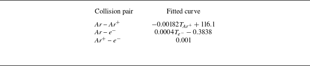For the mixed species collisions $\textit{Ar}$ – $\textit{Ar}^+$ , $\textit{Ar}$ – $e^-$ , $\textit{Ar}^+$ – $e^-$ , cross-sections are described by fitted curves from Devoto (Reference Devoto1973), as shown in table 2, for complex scattering mechanisms such as polarisation and charge-exchange effects that are not captured by simplified collision models. Electron mass was artificially increased ( $m_{\textit{Ar}^+}/m_{e^-}=10$ ) to be computationally tractable. This modification, however, reduces the electrical conductivity. Therefore, the magnetic field magnitude is artificially increased, following the scaling by the similarity parameter $S= {\sigma ^{\textit{cond}}|\boldsymbol{B}_0|^2L_0}/{\rho _0 |\boldsymbol{U}_0|}$ , see more explanation in Appendix A. Sensitivity experiments are performed for mass ratios from 10 to 40 at a fixed magnetic field strength of $B_{\textit{max}} = 0.223$ T. As shown in figure 5, the number density profile of Ar exhibits only minor variations across the range considered, supporting the validity of this approach. To access the convergence status of simulations, we monitor the temporal evolution of averaged key surface quantities, specifically pressure and heat flux. The simulation is considered converged when these monitored quantities stabilise, indicating the absence of significant change.

Table 2.

Cross-section of Ar–Ar ⁺, Ar–e ⁻, Ar ⁺–e ⁻ (unit is Å $^2$ ).

Figure 5.

Comparision of the number density profile of $\textit{Ar}$ in the different mass ratios ( $B_{\textit{max}}=0.223T$ ).

Figure 6.

Contour plots without external magnetic field (upper) and with external magnetic field (lower) in the figures, where the first row is the mass density of (a) $\textit{Ar}$ , (b) $\textit{Ar}^+$ , (c) $e^-$ ; the second row is the x-velocity of (d) $\textit{Ar}$ , (e) $\textit{Ar}^+$ , ( f) $e^-$ ; and third row is the temperature of (g) $\textit{Ar}$ , (h) $\textit{Ar}^+$ , (i) $e^-$ at $B_{\textit{max}}=0.447\,\mathrm{T}$ .

Figure 7.

Contour plots of (a)–(d) electric field magnitude $|\boldsymbol{E}|$ and $E_x, E_y, E_z$ , (e)–(h) current density magnitude $\boldsymbol{J}$ and $J_x, J_y, J_z$ , (i)–(l) Lorentz force magnitude $|\boldsymbol{F}|$ and $F_x, F_y, F_z$ at $B_{\textit{max}}=0.447\,\mathrm{T}$ . Upper and lower figures refer to the results without and with external magnetic fields.

Figure 8.

(a) Number density and (b) normalised x-velocity of ions along the stagnation line with and without applied magnetic field $B_{\textit{max}}=0.447\,\mathrm{T}$ .

Current formulation allows for the observation of distinct behaviours among atoms, ions and electrons, including velocity and temperature slip arising from rarefied effects. Figures 6 and 7 display contour distributions, with upper halves showing simulations without an external magnetic field and lower halves depicting results with background magnetic field strengths ( $B_{\textit{max}}=0.447$ T). The data confirm that an applied magnetic field enhances shock standoff distance.

Figures 6(b) and 6(c) demonstrate that after the application of a magnetic field, both ions and electrons are significantly trapped near the stagnation point. The corresponding number density profiles of ions and electrons along the stagnation line are shown in figure 8(a). These profiles clearly indicate an increase in number density for both species following the application of the magnetic field. This increase occurs because the strong magnetic field in this stagnation region substantially suppresses transverse particle motion compared with the field-free condition. Consequently, charged particles are transported more directly to the wall, elevating the local number density. In contrast, within the shoulder region (the shoulder region comprises arc degrees spanning from approximately $30^\circ$ to $60^\circ$ , with the stagnation line serving as the $0^\circ$ reference), the Lorentz force exerts a greater influence, deflecting charged particles away from the wall and resulting in a lower number density relative to the non-magnetic case, as evidenced in figures 6(b) and 6(c). The collision coupling between these charged particles and argon atoms then contributes to a slight accumulation of argon atoms in the stagnation region, as depicted in figure 6(a). Figures 6(d), 6(e) and 6( f) present the x-velocity of $\textit{Ar}$ , $\textit{Ar}^+$ and $e^-$ . In the stagnation region, $\textit{Ar}^+$ velocity closely follows $\textit{Ar}$ velocity. In the shoulder region, outside of shock, their velocities diverge due to the magnetic field influence on $\textit{Ar}^+$ . Electron velocity deviates significantly from heavy particles as the magnetic field more easily accelerates them and the velocity decoupling is further promoted by low collision frequencies in rarefied environments. Figures 6( g) to 6(i) show similar decoupling in temperature.

The present formulation also permits the observation of electric fields generated by diverse mechanisms. Figures 7(a) depict the electric field magnitude with and without an external magnetic field. In the absence of a magnetic field, the electric field remains generally weak, with localised peaks arising near the walls from sheath formation and across the shock front. Near the wall, the ion density exceeds the electron density, producing a net positive charge that establishes an electric field directed away from the wall to repel incoming ions. Across the shock front, the strong pressure gradient causes charge separation between ions and electrons. Applying a magnetic field alters this structure, shifting the primary electric field peak to the shoulder region. This redistribution is explained by Ohm’s law, $ \boldsymbol{E} \sim \boldsymbol{U} \times \boldsymbol{B}$ , which indicates that the electric field peaks where the cross-product between the electron drift velocity and the magnetic field is maximised, as shown in figure 7(a). Figure 7(e) shows a strong current density concentrated in the stagnation region. The current density here is computed by $\boldsymbol{J} = q_in_i\boldsymbol{U}_{\!i} + q_en_e\boldsymbol{U}_e$ . Figure 7(i) reveals a substantial Lorentz force near this area. The Lorentz force is computed as $\boldsymbol{F} = \boldsymbol{J}\times \boldsymbol{B}$ . The force does not precisely align with the peak current density and magnetic field strength because the magnitude of the Lorentz force $\boldsymbol{J}\times \boldsymbol{B}$ is also critically dependent on the angle between the current density $\boldsymbol{J}$ and the magnetic field $\boldsymbol{B}$ .

Figure 9.

Normalised surface pressure of (a) $\textit{Ar}$ , (c) $\textit{Ar}^+$ , (e) $e^{-}$ and surface heat flux of (b) $\textit{Ar}$ , (d) $\textit{Ar}^+$ , ( f) $e^{-}$ at $B_{\textit{max}}=0.447\,\mathrm{T}$ .

Figure 8(b) displays profiles of the normalised x-component velocity ( $U_x$ ) for ions along the stagnation line (the reference velocity is the free stream velocity). The application of the magnetic field induces additional deceleration. This effect can be attributed to the magnetic mirror force, whereby the magnetic moment $\mu = m v_\perp ^2 / (2|\boldsymbol{B}|)$ – with $v_\perp$ representing the velocity perpendicular to the magnetic field – is approximately conserved in slowly varying fields (Lee, Kim & MacCormack Reference Lee, Kim and MacCormack2015). As charged particles approach the wall, converging magnetic field lines convert perpendicular kinetic energy into parallel motion, resulting in deceleration along the stagnation line. The corresponding reorganisation of electron flow is illustrated in figure 10, where initially smooth streamlines (panel a) become disordered under magnetisation (panel b).

Figure 9 presents the normalised surface pressure and heat flux distributions for $\textit{Ar}$ , $\textit{Ar}^+$ and $e^{-}$ . The reference value for surface pressure and heat flux are $\rho _{\textit{Ar},\infty } U_{\infty }^2/2$ and $\rho _{\textit{Ar},\infty } U_{\infty }^3/2$ , where $\infty$ represents free stream value. Figure 9(a) illustrates that the surface pressure of $\textit{Ar}$ increases near the stagnation region and decreases in the shoulder region. A similar trend in surface pressure is observed for $\textit{Ar}^+$ . Figure 9(b) shows a decrease in heat flux near the stagnation region for $\textit{Ar}$ , attributable to an enlarged standoff distance leading to a smaller temperature gradient. In contrast, the heat flux of $\textit{Ar}^+$ increases in the stagnation region, potentially due to much higher number density near the wall surface caused by the magnetic field and direct energy input from the magnetic field. The pressure and heat flux distribution of $e^{-}$ is similar to $\textit{Ar}^{+}$ . Given that the mole fraction of $\textit{Ar}^+$ is only 0.00623, the overall surface pressure and heat flux are predominantly governed by $\textit{Ar}$ . The observed increase in stagnation pressure and decrease in heat flux on the hemisphere’s surface are consistent with most established literature in this field (Bush Reference Bush1958; Poggie & Gaitonde Reference Poggie and Gaitonde2002; Fujino et al. Reference Fujino, Yoshino and Ishikawa2008).

Figure 10.

Streamline of electron near the wall (a) without magnetic field and (b) with magnetic field $B_{\textit{max}}=0.447\,\mathrm{T}$ .

Figure 11.

Changes in shock standoff distance as a function of magnetic field strength for Mach 4.75 pre-ionised argon flow around a hemispherical geometry (Cambel Reference Cambel1967) (experimental uncertainties is $\pm 10\,\%$ ).

The dependence of shock standoff distance on applied magnetic field strength is presented in figure 11. The shock front location is determined using the density jump ratio, which is defined as (Bisek et al. Reference Bisek, Boyd and Poggie2010)

(3.2) \begin{align} \lim _{M_1\rightarrow \infty } \frac {\rho _2}{\rho _1} = \frac {\gamma + 1}{\gamma - 1}. \end{align}

Here, $M_1$ denotes the upstream Mach number, $\gamma$ represents the ratio of specific heats, $\rho _1$ is the upstream density and $\rho _2$ is the downstream density. For argon gas, with $\gamma _{\textit{Ar}} = 5/3$ , this density ratio is calculated to be 4. Our simulations exhibit good agreement with experimental data. (The experimental uncertainty arises from limitations inherent in the measurement technology.) In addition to experimental results, reference simulation data from Bisek et al. (Reference Bisek, Boyd and Poggie2010), employing three distinct conductivity models, are included for comparison. The primary distinction between the present formulation and Bisek’s work lies in our consideration of non-equilibrium transport phenomena in ionised gases, whereas Bisek’s results are based on the MHD equations. For hypersonic flow around a hemisphere, the standoff distance increases with increasing Knudsen number when rarefied effects are significant (Long et al. Reference Long, Wei and Xu2024).

3.2. Control effects under different Knudsen numbers

This subsection investigates the influence of control parameters across varying Knudsen numbers (0.2, 0.08, 0.044 and 0.02). The Knudsen number is determined by the incoming argon gas density, which is set to 2.18 $\,\times\,\text{10}^{-5}$ kg $\,$ m $^{-3}$ for Kn = 0.2; 5.45 $\,\times\,\text{10}^{-5}$ kg $\,$ m $^{-3}$ for Kn = 0.08; 1.09 $\,\times\, \text{10}^{-4}$ kg $\,$ m $^{-3}$ for Kn = 0.044; and 2.18 $\,\times\,\text{10}^{-4}$ kg $\,$ m $^{-3}$ for Kn = 0.02. The computational geometry, meshing and other detailed parameters remain the same as in the prior section. The similarity parameter, $S$ , is held constant across these variations in Knudsen number. According to (A3) and (A5), shown in (A3), if the argon atom density increases by a factor $a$ , the parameter $S$ inherently decreases by a factor $a^2$ . To counteract this effect and maintain a constant $S$ , the magnetic field magnitude $|\boldsymbol{B}|$ must be amplified by the same factor $a$ . The magnetic field magnitude in this section is set to be $B_{\textit{max}}=0.447\,\mathrm{T}$ .

Figure 12.

Temperature contour plots of the argon atoms at (a) Kn = 0.02, (b) Kn = 0.04, (c) Kn = 0.08, (d) Kn = 0.2 at $B_{\textit{max}}=0.447\,\mathrm{T}$ . Upper and lower figures refer to the results without and with external magnetic fields.

Figure 13.

Local Knudsen number contour plots of the argon atoms at (a) Kn = 0.02, (b) Kn = 0.04, (c) Kn = 0.08, (d) Kn = 0.2 at $B_{\textit{max}}=0.447\,\mathrm{T}$ . Upper and lower figures refer to the results without and with external magnetic fields.

Figure 12 displays the argon atom temperature field at various Knudsen numbers. The shock front exhibits a sharpening trend as the Knudsen number decreases. Figure 13 displays the local Knudsen number of an argon atom to illustrate the transport non-equilibrium of an argon atom. The local Knudsen number is defined as $Kn_{local} = {\lambda }/{\rho /|\boldsymbol{\nabla }\rho |}$ , where $\lambda$ is local molecular mean free path; $\rho$ is the mass density. The plot shows that the overall Knudsen number increases throughout the domain as the reference Knudsen number rises. In particular, at a higher Knudsen number as Kn = 0.2, the local Knudsen number inside the shock wave remains comparable in magnitude to that outside the shock, indicating a non-equilibrium state even within the shock region itself.

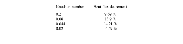
Figures 12 and 13 show that the standoff distance increment reduces with increasing Knudsen numbers. As a result, the total heat flux decrement also exhibits a decreasing trend with larger Knudsen numbers, as shown in table 3 and figure 14. The heat flux is calculated by integrating over the entire wall surface area. This phenomenon is due to the enhanced decoupling between atoms and charged particles at higher Knudsen numbers. The normalised x-velocity and temperature profiles along the stagnation line are shown in figures 16 and 15, respectively. The referenced values are free stream velocity and temperature. As illustrated, the velocity and temperature differences between atoms and ions grow progressively larger with increasing Knudsen number, reflecting a more pronounced departure from equilibrium. This trend arises from the inverse relationship between the Knudsen number and number density: at higher Knudsen numbers, lower atom densities reduce the collision frequency between atoms and ions. Conversely, as the Knudsen number decreases – corresponding to increased atom density – collisions become more frequent, driving the velocities and temperatures towards equilibrium.

Table 3.

Heat flux decrement with varying Knudsen number.

Figure 14.

Heat flux decrement percentage as functions of the Knudsen number.

Figure 15.

Normalised temperature profile of argon atom and argon ions along the stagnation line at (a) Kn = 0.02, (b) Kn = 0.04, (c) Kn = 0.08, (d) Kn = 0.2. The temperature difference $\Delta T = T_{\textit{Ar}^+} - T_{\textit{Ar}}$ is also shown as grey dots.

Figure 16.

Normalised x-velocity profile of argon atom and argon ions along the stagnation line at (a) Kn = 0.02, (b) Kn = 0.04, (c) Kn = 0.08, (d) Kn = 0.2. The temperature difference $\Delta U_x = U_{\textit{Ar}^+,x} - U_{\textit{Ar},x}$ is also shown as grey dots.

Figure 17.

(a) Maximum normalised velocity difference and (b) maximum normalised temperature difference along the stagnation line between atoms and ions as functions of the Knudsen number.

Figure 17 presents the maximum velocity difference (panel a) and maximum temperature difference (panel b) between atoms and ions as functions of the Knudsen number. Both differences increase approximately linearly with the Knudsen number. This linear trend corresponds directly to the observed reduction in surface heat flux with increasing Knudsen number in figure 14, confirming that higher rarefaction leads to greater departure from equilibrium between charged and neutral species. Figure 18 further illustrates the x-velocity of argon atoms with and without an applied magnetic field. The magnetic field significantly decelerates the argon atoms, but the magnitude of this deceleration diminishes as the Knudsen number rises. Consistent with the previous discussion, the enhanced decoupling at higher Kn weakens the drag exerted by the charged species on the neutrals, thereby reducing the deceleration effect. This mechanism explains why higher Knudsen conditions attenuate the electromagnetic control effectiveness. In summary, increasing the Knudsen number enhances the decoupling between charged and neutral particles, which in turn weakens the efficacy of electromagnetic control.

Figure 18.

Normalised x-velocity profile of argon atom with and without the applied magnetic field along the stagnation line at (a) Kn = 0.02, (b) Kn = 0.04, (c) Kn = 0.08, (d) Kn = 0.2. The velocity difference is plotted as grey dots.