Introduction

Surface velocity is one of the most important glacier variables to measure for studies of dynamics. The aim of this paper is to demonstrate methods of measuring glacier velocity by using sequential photography from a single camera location and to show results obtained in using the method at Columbia Glacier, Alaska. The method was specifically developed for Columbia Glacier to fulfill a need for short-interval velocity measurements at its terminus. It can provide ice velocities and changes in terminus positions with daily resolution. Because the calving velocity is the difference between these two quantities, it can also be obtained with the same time resolution. The calving velocity can then be used with data for other variables, e.g. fresh water run-off, tide stage, glacier thickness, in investigating the calving mechanism (Reference Brown, Meier and PostBrown and others, 1982; Reference SikoniaSikonia 1982).

A large amount of surface-velocity data from the terminus of Columbia Glacier has been obtained. Beginning in 1976, vertical aerial photography has been obtained over the lower reach at time intervals of one to four months. By standard photogrammetry, the coordinates of seracs or crevasse intersections can be obtained. The same feature can usually be found on photographs from each of two successive flights and the displacement between the two positions can be used to determine the average velocity for the time interval. The accuracy of measurement of these horizontal displacements is about 4 m; considering the average velocity and interval between flights, the mean error in velocity is about two per cent. The data from July, 1976 to September, 1981 show: 1) at km 66 (about 0.5 km above the 1983 terminus position), velocity reaches a seasonal maximum of about 8.2 m/day in mid-fall and a seasonal minimum of about 2.7 m/day in late spring; 2) the velocity increases with distance from 60 to 66 km by about 100 per cent; 3) the terminus position changes seasonally by about 300 m, with a minimum glacier length in late fall and maximum length in early summer. These data are described in detail by Reference Meier, Rasmussen and MillerMeier and others (1985a). Major limitations of the aerial photogrammetry are the many-week time resolution and coarse spatial resolution close to the terminus. Furthermore, the expense of the photography and photogrammetry is high.

A few features on the lower glacier have been surveyed by traditional triangulation or foresight methods, but the results have been limited to several kilometers above the terminus with several-month time resolution. To use traditional methods of surveying near the terminus for more than a lew weeks would be extremely expensive. A 16 mm movie camera, overlooking the terminus, has been in operation since early 1978. When one frame per day is projected at high speed, say 6 frames per second, the ice movement is obvious. However, when the frames are taken individually, the dominating feature of the image is that of film grain and generally low resolution. When shown in rapid sequence, a mental pattern-recognition is applied to the frames, which is difficult to carry to individual scene pairs for quantitative displacement measurement, and thus no short-term velocities have been obtained from 16 mm film. The possibility of making velocity measurements was obvious, though, and a 35 mm sequence camera system was designed and installed specifically for the purpose of measuring short-term ice velocity. Velocity has also been successfully measured on other glaciers using small-format cameras (Reference Iken, Röthlisberger, Flotron and HaeberliIken and others, 1983).

The Camera, General Geometry, Landmarks and Image Sets

A motor-driven, electrically-triggered 35 mm-format camera with a 30 m film reel, was installed in early 1983,overlooking the Columbia terminus (Fig.1). The camera, a HulcherFootnote * model 112, is mechanically robust and electronically simple as compared to modern 35 mm cameras. In practice, it was dependable, but difficult to load. Failures of the system were due either to faulty charging or faulty film loading. The camera, timer solar array voltage regulator, 8 amp-hour, lead-acid battery and weather-protecting window box were mounted on a 2 m high tower, made from heavy aluminium angle. The interior of the four legged tower was filled with rocks, for stability. The exposure time was determined with knowledge of beginning and end times, the use of a crystal-controlled timer, and the frame count. Three frames were to be taken each day (8, 12, and 16 hours), color or black and white film was used during different periods, and the exposure was pre-set for an average sunny day.

Fig. 1

The lower Columbia Glacier, camera view, and coordinate system. The coordinate system is with the camera at origin, north is y positive, east is x positive. UTM and lat.-long. ticks are also shown. The solid triangles within the camera are the landmark points. The sample trajectory is shown by an arrow near x = -5800, y = 0.

The camera was located and oriented so that several requirements could be met, The terminus must be observable; the velocity vectors should be nearly norma! to the direction of view; the location should be such that the elevation angle to the ice-mass surface is large, but should still be relatively close to the ice-mass; and land reference should be visible (Fig.1.). Assuming a directionally-stable camera, it is not essential to have absolute orientation to determine relative positions in any particular view, but it is desirable so that the true space locations of targets can be determined. Several landmarks that could be identified on the film were surveyed for precise positions. These landmarks were specific tree tops, rocks, artificially marked points and a mountain peak on the distant horizon. The positions of all the landmark points were determined to ±10 cm, except the peak, which was not surveyed and was known to only ±100 m. The camera location was also surveyed to ±10 cm.

Under ideal conditions, an automatic camera could give an unbroken set of data. In practice, when the visual objective is more than a few meters away, weather conditions usually cause breaks in the record. A weather-dependent system such as this may produce data gaps at critical times, e.g. during periods of high precipitation, when velocity is known to increase (Reference VaughnVaughn and others, 1985).

During 1983, the system operated from January 8 to April 25, May 24 to June 2, and July 27 to November 13. A usable, mid-day photograph was obtained on 65, 10, and 64 days, respectively, during those periods.

Photograph Digitization and Data Transformation Scheme

The usable photographs were enlarged so that the long axis was about 49 cm. This particular enlargement was used only because it conveniently fitted the digitization tablet that was used. The analysis algorithm allowed for variable scale; thus, the exact enlargement coefficient was not critical and variation between photographs was acceptable.

Several sets of data were extracted from each photograph by using a.127 mm resolution digitization tablet. The tablet coordinates of 12 photograph edge points, from 2 to 7 landmark points, up to 40 points on the glacier surface and up to 100 points at the ice/water intersection (terminus) were measured for each photograph. The 12 edge points (three, widely-spaced, along each edge of the photograph) were used to define the center of the photograph by calculating the two orthogonal sets of parallel lines best fitting the edge points, then by calculating the center of the rectangle formed by the four lines.

The transformation of photograph plane coordinates to true space location of targets is a several-step process. This includes: 1) locating the center of the photograph, 2) calculating the orientation of the camera, 3) calculating the direction numbers of the rays from the camera to the targets, and 4) calculating the true location of the points by using an approximated glacier surface topography.

Direction Numbers from an Oblique Photograph

It is not possible to determine the absolute coordinates of a point from the position of its image in oblique photographs taken from only one location. Only the orientation of the straight line passing through the point and through the center of the camera lens may be determined. Some other condition is needed to determine the point’s location along this line.

At the time of an exposure, the image of the field of view is inverted as the straight fines pass through the lens to the film bed. When the film is processed, the inverted image on the negative is re-inverted to produce a true image on the photograph positive. Following Slama (Reference Slama1980, section 2.2.2), the transformation derived here is for the photograph positive, which is visualized to be on the same side of the lens as the field of view. If the photography is assumed to follow a central projection, i.e. a point’s location is assumed to be co-linear with its image on the photograph and the center of the lens, and if the location and orientation of the camera are known, then the photograph coordinates of its image may be transformed, linearly, into the direction numbers of the straight line passing through the point.

The formulation given here for the transformation is equivalent to that given by Slama (Reference Slama1980, eq. 2.22), but it is expressed in terms more appropriate for oblique photography of glaciers. The camera is taken to be at the origin of a right-handed coordinate system (x, y, z), and the orientation of the optical axis is defined by its azimuth angle, θ, and by the elevation angle, φ, above the horizontal (Fig.2).

Fig. 2

Oblique photography coordinate system. For Columbia Glacier data, the x-axis is taken to be positive to the east, the y-axis to the north, and the z-axis upward.

The plane that is parallel to the photograph but is a unit distance away from the origin is

in which

is its photogrammetric principal point, i.e. the point nearest the origin, where the optical axis intersects the plane. The central projection (X_i, Y_i, Z_i) onto this plane of a landmark point with known coordinates (x¡, y_;i z_i) is given by

In this plane, a right-handed coordinate system is positioned with (0, 0) at (x_o, y_o, C_o), with the along the intersection of the plane and the horizontal plane z = z_O, and with the in the plane and directed above the horizontal plane. The projection (X_i, Y_i, Z_i) then has coordinates

The plane of the photograph is

in which is the principal distance of the photograph; it is the distance from the camera to the principal point of the photograph (σχ_o, σy_o, σz_o), and is equal to the focal length of the lens times the enlargement factor of the photograph. The position of an image is defined by a right-handed coordinate system (λ, μ), having its origin at the principal point, which is taken to be at the center of the frame, and having arbitrary rotation φ from the horizontal (Fig.3). The and (λ_i, μⁱ) coordinates of a straight line through some point (x_i, y_i, z_i) are then related by the scaling-rotation.

Fig. 3

Image coordinate system. The origin is at the principal point of the photograph, which is approximated by the center of the frame. Its arbitrary orientation is defined by the angle of rotation φ from the intersection of the photograph with the horizontal (z=constant) plane through the principal point.

The desired transformation is obtained by solving equations 4 and 6 for the direction numbers in terms of the photograph coordinates

The transformation has four parameters, θ, φ, Φ, and σ which, in principle, could be determined directly by measuring the orientation of the camera, but a much more accurate calibration can be obtained by determining them empirically from the coordinates of landmark points. If the coordinates (x_i, y_i, z_i) are known for several landmark points, of which the image position (λ_i,μ_i) can be measured on a photograph, then the values of the four parameters may be estimated by a least-squares minimization process. A closed-form expression cannot be given here for simultaneously determining all four parameters, but the process may be divided into a direct part, for getting φ and σ, within a well-behaved iterative part, for getting θ and Φ. Because observation errors occur in measuring both a landmark’s actual position and its photograph coordinates, the more landmarks that are used, the better the calibration will be.

For trial values of θ and Φ, the optimum values of the principal distance σ and the orientation φ of the μ system are given directly by

in which the summations are over the n landmark points used, and eq. 2-4 are used to get from (xⁱ, yⁱ, zⁱ). The products σcosφ and σείηφ are readily decomposed by using the relations σ =[(σcosφ)² + (σsinψ)²]^½, then sinφ = (σsinψ)/σ and cosψ = (σcosψ)/σ. The values of σ and ψ produced by equation 8 are the ones that minimize the root-mean-square instance Ep between the (λ_i, μ_i) and the coordinates ( ) actually measured on the photograph; that is,

The absence of weights reflects the assumption that for all n points the errors in measuring come independently from the same distribution.

Because the foregoing algorithm (eqs. 2-4, 6, 8) is performed for particular trial values of θ and φ, the distance Ep is also a function of those two angles. The minimum value can easily be found iteratively by using as a first approximation, the values of the angles estimated in the field. When plotted as a function of θ and φ, constant Ep contours for Columbia Glacier data closely resemble concentric circles and, as would be expected from the mathematics, the plot was unaffected by changing the orien¬tation of the λ, μ coordinate system on the photograph, If n=l, the solution İs underdetermined; for any θ and φ, there exist values of σ and Φ that make Ep=0. If n=2, the transformation is uniquely determined, i.e., there exists one set of values for the four parameters that produce Ep=0, but all the errors in measuring the are fully incorporated into it. Only if n ≥3 is there any least-squares reduction of the effect of the measurement errors and the optimum values of the four parameters occur with E_p>0 if the contain errors and E_p=0 if they do not.

In the case of the camera installation at Columbia Glacier, it was not certain that the camera orientation was stable and thus θ and Φ were calculated separately for each of 40 photographs between July 27 and September 19. Of the seven landmark points, several combinations were used for the θ, φ iteration depending on which were identifiable in a given photograph. Typical Ep values were between 0.3 and 0.9 mm. E_p can be related to angular measurement by scaling the known angular span of the image to the size of the image. The photograph spans 19.5 and is 490 mm across. Using this relationship and 0.5 mm as an approximate Ep, then the typical error is in the order of 0.02°. This agrees with the standard deviation of the 40 θ values (δ_θ = 0.022°) and φ values (δφ = 0.011°). It was found that the distribution of θ and Φ was clustered in two groups, and that the clustering corresponded to the inclusion or not of the distant peak in the data set. The peak’s position was not well known, and when it was eliminated from the set δ_θ = 0.006° and δ_φ = 0.013° resulted. Considering 19 photographs, all with the same five landmark points, the standard deviations of θ and Φ further improved to δ_θ = 0.0053° and δ_θ = 0.0089°.

The errors in the θ and Φ camera orientation angles actually represent the sum of the errors of locating points on the photograph, digitizing their locations, and finding the photograph center. The θ and Φ error is a result of a least-squares minimization of the location of up to six landmark points and is considered to be an indication of the degree of stability of the system, i.e., does the camera move from day to day? It is also the best indication of the ultimate precision that can be expected in using this particular high quality, “off the shelf”, 35 mm camera, paper enlargements from a standard enlarger, and a 0.127 mm resolution digitization tablet. The angular measurement errors are approximately one order of magnitude less precise than a high quality theodolite could produce.

Absolute Coordinates from the Direction Numbers of an Image

If the topography of the terrain in the field of view is known, then absolute coordinates may be determined for points whose images appear in a calibrated, oblique photograph. Letting a region of the terrain be approximated by a plane

the direction numbers of a line X, Y, Z obtained from equation 7 for some measured image position λ, μ can be converted to the point 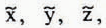, where the line intersects the plane

For points at the glacier terminus, the horizontal plane representing sea level is used. For points on the glacier surface, the terrain is approximated by a piece-wise planar surface in which each triangular segment is defined by the plane passing through its vertices (x₁ y₁ z₁), (x₂ y₂, z₂), (x₃, y₃, z₃); then the coefficients are given by

The projection 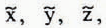is in the plane, but it may or may not be in the triangular segment determined by the three points. Because it is in the plane, it may be expressed as a linear combination of the three points

The weights, whose sum is unity, are given by

in which M’ is the transpose of the matrix M. The condition that be in the triangle is min. (q_j)>0. If mín. (q_j)=0, it is on an edge of the triangle (if two of the qj are zero, it is at a vertex) and, if min. (q_j)<0, it is outside the triangle. This formulation is restricted to the condition where the plane is not vertical, which is suitable to approximating a glacier surface and is computationally much simpler than a generalized formulation, not subject to this restriction. Except for those planes that might be parallel to it, the line will intersect every plane used to approximate a glacier surface.

Examining the weights, q_j, will eliminate most, but not necessarily all, of the spurious intersections. A line nearly parallel to the mean trend of a rough surface might intersect it in several places: entering the surface, emerging from it, re-entering it, etc. Only the first of such multiple valid intersections, the one nearest the camera, would be the one visible in the photograph.

Calculating Particle Trajectories

The trajectory can be calculated for a point on the glacier surface, if it appears on many calibrated photographs taken over a period of time. Equations 7 and 11 are used to estimate its absolute coordinates 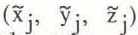from its image position on photographs taken at times t_j. Because the coordinates are subject to several sources of error (in calibrating the photographs, in approximating the glacier surface, in measuring the point’s image), it is necessary to smooth the . For the length of time that an individual point is visible in the oblique photographs at Columbia Glacier, its sequence of 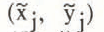exhibits a linear trend, but with considerable scatter (fig.4).

Fig. 4

A sample trajectory. The open circles indicate calculated positions on the horizontal plane of one target for July 27 to September 19, 1983. The solid circles indicate the positions of the target after they are projected (equation 18) toward or away from the camera on to the line best defined by all the positions (range-sense fit). There are two errors associated with each open circle. The first, about 15 m in x (indicated by a bar at one point) and 1 m in y (one half the size of the open circles) is well defined and is the result of imprecisions within the overall optical and measurement system. The second is the result of the inaccuracy in the piece-wise planar approximation of the glacier surface, which varied as the surface altitude changed during the measurement period. This error is systematic and does not dramatically influence the resulting velocities. It is assumed that the trajectory is linear over the observed distance and time.

Comparisons of the scatter of one trajectory with that of another reveal a poor correlation, which suggests that the largest contribution to the scatter is caused by errors in measuring (λ^* μ^*). A consideration of the geometry of the intersection of a line with the plane approximating the glacier surface indicates that small errors in the line’s direction numbers will produce much larger errors in the range of the calculated intersection point (that is, its distance from the camera, given by than in the transverse direction. The direction numbers of a line, which come from its photograph coordinates, define its azimuth angle θ and elevation angle Φ. Thus, errors in λ^*, μ^* produce corresponding errors in θ and φ. If φ is the elevation angle referred to the approximating plane, instead of the horizontal, then the range error is . The transverse error is . For = 5000m and φ = 3°, which are typical of the Columbia Glacier data, errors of 0.01° (1.7 x 10⁻⁴ radians) in φ and θ yield position errors d = 17 m and d = 1 m.

Because the range errors are so much greater than the transverse errors, an uncommon least-squares method for fitting a straight line to the is used. The common, ordinate-sense fitting (in which residuals in the direction of a particular coordinate axis are minimized) is rejected because the result is not independent of the coordinate system. The little-used, normal-sense fitting, in which residuals in the direction normal to the line are minimized, is independent of the coordinate system, but, for the Columbia Glacier data, that direction often does not align well with the direction of the range errors. Instead, rangesense fitting is used. Unfortunately, a direct method cannot be given here for getting the optimum line, which is a dis¬advantage of this method compared with the other two.

Letting the required line be written as

the quantity to be minimized is

over the N points to which the line is to be fitted. Here is the relative adjustment of the range, and r_j is the norizontal range to 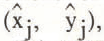which is the horizontal central projection of onto the line (fig.4), and is the horizontal range to . The projection is given by

Because a direct method cannot be given here for simultaneously determining the values of A, B, and C that minimize E_T, a wetl-behaved iterative procedure with only one degree of freedom is used. The ratio is equal to the factor in equation 18. For fixed A and B, then, requiring ∂E_T/∂C = 0 yields

Equation 16 may be arbitrarily multiplied by a constant, so that A and B embody only one degree of freedom, the slope of the line. Thus, equation 19 is used to get the optimum value of C, as the slope is varied, until E_T is minimized. The procedure is restricted from using any slope, if a line with that slope through (x, y) = (0, 0) would pass through any of the ; that is, 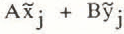must be non-zero for all j.

Trajectories and Velocities

The altitude of the glacier surface, at the intersection of the ray, strongly affects the calculated position of the target. Fortunately a topographic map from September 16 1983 vertical, aerial photography was available for the region of interest. This map was used to determine 13 triangular segments to approximate the topography. If it is assumed that the glacier topography remains constant (an unlikely situation) throughout the period of observation, but there was an altitude error Δz that was constant in x and y, then the set of trajectory points would simply be displaced radially, toward or away from the camera a distance of Δζ/tan . The only test made for this error was a subjective placement of a trajectory on the September 16 1983 map by using vertical photography from the same date as an aid. This was done by placing, on a map, features that could be identified on both the oblique and vertical photographs. In most cases the subjectively placed trajectory was within 200 m of the calculated trajectory. The effect of this error would be a minor scale change in displacements along the trajectory and subsequent minor velocity errors.

The second potential error occurs when the altitude of the surface is changing during the observations. This would result in an apparent rotation of the trajectory, or an error in the direction of flow. It is known that the surface altitude was changing during the summer and fall of 1983, generally decreasing (Reference Meier, Rasmussen and MillerMeier and others, 1985b). The test of this error was again subjective; if the trajectory direction did not approximately correspond to that as determined by the sequential vertical photogrammetry methods (Reference Meier, Rasmussen and MillerMeier and others, 1985a), then the trajectory was considered to be unreliable. Three trajectories, all very near the terminus, where the surface altitude was changing very rapidly, showed unlikely direction.

A third potential error occurs if a target moves through an area of the glacier that is estimated to be planar, but is actually a series of dips and swells. This could result in a meandering x position of the target and may be the reason for the gross shape seen in Figure 4. The range-sense fitting to a straight line, as described earlier, was designed to eliminate this problem. Furthermore, the gross x, y shapes of the nearby trajectories were not similar, while their t, v plots usually were similar, indicating that the velocity fluctuations are a function of y position or time, not error in the x position.

The positions ŷ on the radially best fitting trajectory, along with their time coordinates, can be used to calculate velocity. The simplest velocity calculation, to give v = dŷ/dt at t = (t_j+1 + t_j)/2, is

Because the trajectory is assumed to be linear (equation 16), the two components are related by

in which 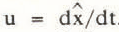. Typical velocities during the measured period were 6–8 m/day. The typical error along the trajectory was 1 m, so that daily velocity measurements appeared to be quite noisy. Furthermore, comparison of different trajectories was complicated because they had differently timed intervals; in other words, all features were not visible in all photographs. It was desirable to make all trajectories continuous throughout their total period of record, with a datum point on each day.

A superior method of fitting the N points (t, ŷ) is the cubic spline f(t), which consists of a separate cubic polynomial on each time interval [t_j, t_j+1], which is continuous in function value and first two derivatives, and which is smooth because it minimizes the integral

A cubic spline smoother than the one passing exactly through the (t, ŷ) can be obtained (Reference ReinschReinsch, 1967) by specifying an error E_y. In addition to having the properties stated above, the smoothing spline also obeys

Of all the cubic splines obeying equation 23, the one that gives the minimum value of I is obtained.

Although a separate error (E_y)_j may be ascribed to each ŷ_j in forming the cubic spline, a constant E_y value was used in processing the Columbia Glacier data. The smoothing spline for E_y = 1 m, as fitted to the points on the trajectory of Figure 4, is shown in Figure 5.

Fig. 5

The y displacement, as a residual from the linear time trend, for the trajectory of Fig.4. The open circles indicate the y of each range-fit target position. The solid line indicates the smoothed cubic spline. The error assigned to each y was 1 m.

Because the spline f(t) gives the y-displacement, its derivative df(t)/dt gives the v-component of velocity. The v(t) curve obtained from the f(t) curve of Figure 5 is shown in Figure 6, along with v(t) curves obtained from smoothing splines fitted to the same (t, ŷ) data for E_y = 0.5, 0.8, and 2.0 m.

Fig. 6

Velocity versus time for the trajectory of Fig.4. Velocity is obtained by differentiating the spline. Each v(t) curve is identified by the error that was ascribed to each y-value when the smoothing spline was fitted to the (t, ŷ). The I m curve is the derivative of the cubic spline in Fig.5.

The v(t) curve obtained from a spline fitted to the (t, ŷ) data applies to an individual target as it moves through space and time. If spline fits are made for many targets, then, in principle, v(x, y) and u(x, y) plots can be constructed for some particular t. For each target the smoothing spline f(t) gives y and the derivative df(t)/dt gives v; from y equation 16 gives x and from v equation 21 gives u. Also, v(t) curves at some point (x, y) fixed in space can be obtained by interpolating at that point in successive v(x, y) plots, and similarly, for u(t) at some fixed point. Discontinuities in derivatives introduced when a target passes from one plane to another in the surface approximating the glacier topography may not be entirely removed by the action of the smoothing spline.

Conclusions

Long-term observation of glacier velocity is feasible using monoscopic 35 mm photography, if certain precautions are taken. A stable mounting system simplifies analysts tremendously and is essential if no landmark references are available. A balance of field of view, expected velocities, distance from targets, and lens focal length must be optimized to achieve the desired observations. At Columbia Glacier a 105 mm lens was used about 5 km from the glacier center line to measure velocities of about 8 m/day. Daily displacement of targets was in the order of 100 μm on the 35 mm film. If true target coordinates are to be ssdetermined, the glacier surface topography must be known. Also, camera location should be chosen to give a camera view nearly normal to the ice flow and a camera-to-target altitude difference sufficient to form a “vertical angle” large enough to determine the range to a target. Finally, targets must be visible on the photographs, whether they be naturally occurring features or artificially placed.